
Submitted:
24 March 2023
Posted:
30 March 2023
You are already at the latest version
Abstract
This study examined the spatial-temporal distribution of sulfur and iron compounds (dissolved sulfide, iron sulfide, and ionized iron) in sediments from April 2015 to March 2016 at four stations in Mikawa Bay, Japan. Seasonal changes were observed in dissolved sulfide, iron sulfide, and ionized iron in the upper part of the sediment (0–4 cm depth) at all stations. The maximum concentration in the upper part of the central bay was 2.8 mmol L-1. The maximum values of dissolved sulfide (ranging from 1.4 to 8.1 mmol L-1) at stations located in a water way varied among stations. The iron sulfide concentration in the upper part of the sediment at a station where dissolved sulfide concentration in the waterway was relatively low exceeded that at other stations in the waterway during spring to summer. Ionized iron concentration was highest at the station where the dissolved sulfide concentration was low. The study results suggest that iron plays an important role in determining the magnitude of dissolved sulfide accumulation in sediments by binding with dissolved sulfide. The results imply the possibility of mitigating the accumulation of free sulfides, which causes extreme hypoxia, by artificially adding sufficient iron to the seabed.
Keywords:
dissolved sulfide
; iron
; hypoxia
; buffering capacity
; environmental restoration
; coastal waters
; Mikawa Bay
; dead zone
1. Introduction
For 45 years, a system for the area-wide control of total pollutant load has been established to improve the water quality of enclosed bays in Japan, such as in Tokyo, Osaka, Ise, and Mikawa Bay. The system has led to the steady reduction of chemical oxygen demand (COD), total nitrogen (TN), and total phosphorus (TP) discharged from land areas to these enclosed bays. Nevertheless, severe hypoxia still occurs, and has reduced habitat availability and fishery production in Mikawa Bay during summer [1,2,3]. However, the excessive reduction of TN and TP loads is a causal factor of the decline in fishery resources owing to a continued decrease in their primary production [4].
The critical condition of hypoxia is one of the most serious challenges in Japan [5]. Therefore, Japan's Ministry of the Environment (MOE) used bottom dissolved oxygen (DO) as an index to assess the direct influence of hypoxia on aquatic organisms.
Critical hypoxic conditions occur every summer in Mikawa Bay, a typical closed bay, similar to Tokyo and Osaka bays in Japan. Critical hypoxia is mainly attributed to a considerable reduction in the water purification capability provided by the tidal flat macrobenthos community, which is associated with aggressive reclamation in Mikawa Bay [6,7]. Therefore, tidal flats and shallows are being restored in Mikawa Bay [5]. Intensive reclamation has alleviated water purification capability and created water areas where poor water quality has exacerbated drastically. Waku et al. [8] extended the concept of the dead zone advocated by Diaz and Rosenberg [9] to coastal waters and determined dead zones as local areas where few organisms can survive owing to severe environmental degradation in Mikawa Bay. The dead zone associated with intensive reclamation covers an area of 27.8 km2 around the coastal waters of Mikawa Bay [8]. The upwelling of hypoxic water from the dead zone to the sublittoral zone kills the macrobenthos community, which plays an important role in water purification, and damages the general ecosystem of the bay [10]. Although large-scale ports account for a large portion (79.2%) of the dead zone, effective environmental restoration is difficult.
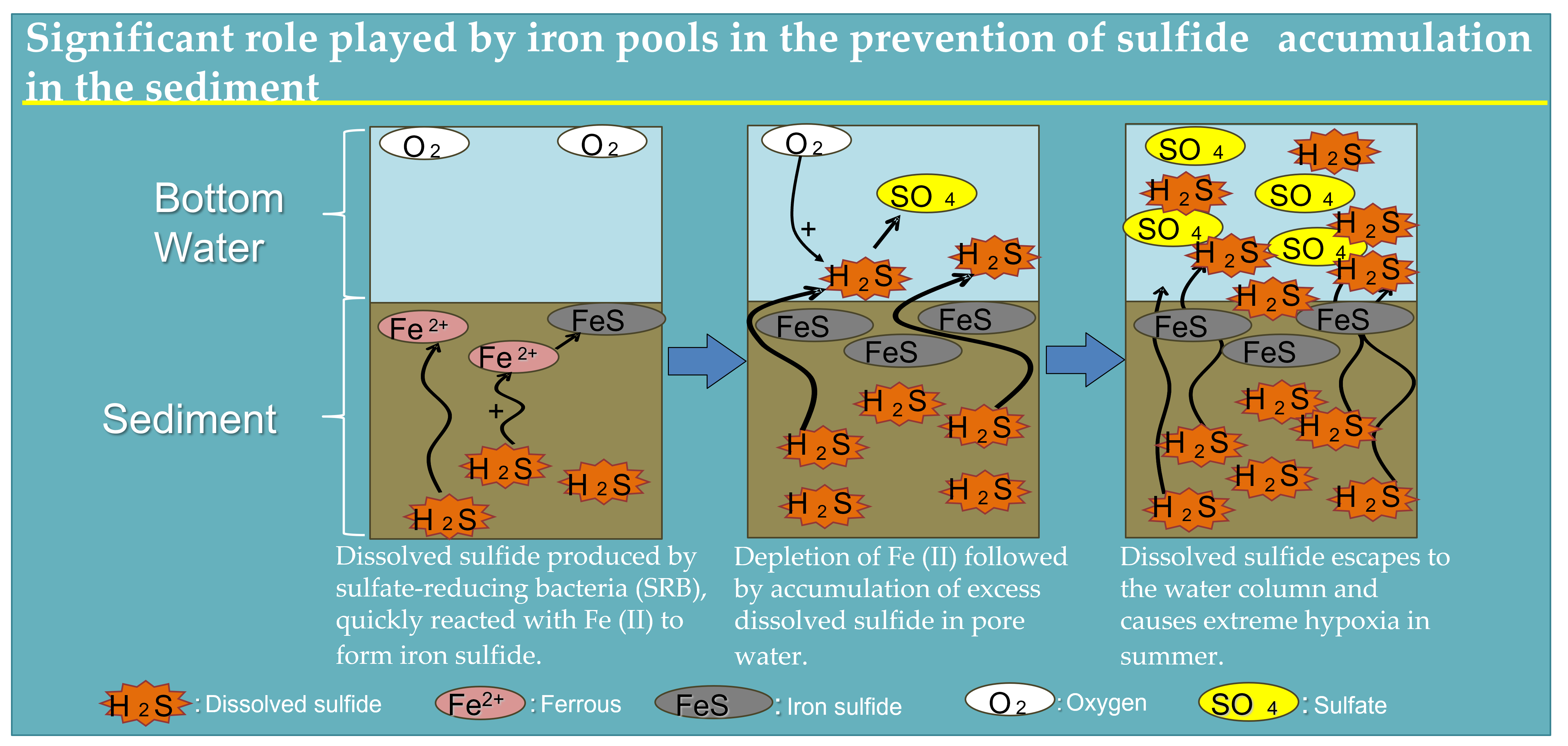
Extreme hypoxia is driven by dissolved sulfide derived from sulfate reduction in the seabed. Dissolved sulfide reaching the surface of sediment escapes to the water column and play as an oxygen consumer that sustains anoxic conditions in the water at the bottom [11,12].
In numerous marine ecosystems, iron is quantitatively the most important metal [13,14], and is highly reactive with sulfide [15,16,17,18]. Although this mechanism can potentially prevent the accumulation of free sulfides in the sediment [13,19,20,21,22], there are only a few studies on sulfur and iron cycles through field observation at dead zones, where environmental restoration is particularly required.
Numerous surveys were conducted from April 2015 to March 2016 to investigate the spatial-temporal changes in sulfur and iron compounds (dissolved sulfide, iron sulfide, and ionized iron) in sediments. In the present study, we describe the effect of iron compounds on the inhibition of dissolved sulfide development, which causes extreme hypoxia.
2. Materials and Methods
2.1. Study Site
Mikawa Bay is an embayment in central Japan (Figure 1). It covers a surface area of 604 km2 and is 9.2 m deep [23]. Our survey was conducted in a closed section of Mikawa Bay, where critical hypoxia occurs from early summer to early autumn annually. Station 1 (Latitude 34 ˚44.60‘ N, Longitude 137 ˚13.22‘E, Chart Datum Level (CDL): -10.0 m) is located in the central part of Mikawa Bay. Stations 2 (Latitude 34 ˚43.82‘ N, Longitude 137 ˚18.29‘E, CDL: -11.5 m), 3 (Latitude 34 ˚42.77‘ N, Longitude 137 ˚18.30‘E, CDL: -10.1 m), and 4 (Latitude 34 ˚41.75‘ N, Longitude 137 ˚18.37‘E, CDL: -8.0 m) are located in a waterway associated with a large-scale port, which is defined as a dead zone [8].
2.2. Field Observation and Sampling
Field observations were conducted at Stations 1, 2, 3, and 4 from April 23, 2015 to March 23, 2016, on a monthly basis except at Station 2 on April 23, 2015 and May 27, 2015.
Seawater temperature, salinity, and DO were measured using a Conductivity-Temperature-Depth profiler (CTD) fitted with a DO sensor (AAQ1182, JFE Advantech Co., Ltd, Nishinomiya, Hyogo, Japan) at depth intervals of 2 m from the surface to the bottom.
Sediment cores were collected by scuba divers who inserted acryl tubes with an inner diameter of 4.2 cm and length of 50 cm into the sediments. Then acryl tubes containing sediments and approximately upper 10 cm of bottom water were capped with rubber plugs on both ends immediately after sampling. Four sediment cores were collected at each station. The cores were stored under dark and cold conditions and transported to the laboratory for chemical analysis.
2.3. Chemical Analysis of Sediment Samples
The top 16 cm of the sediment core was sliced into eight 1-cm slices (0-1, 1-2, 2-3, 3-4, 4-5, 5-6, 9-10, 15-16 cm from the sediment surface) for chemical analysis. The sliced sediment cores were placed in 50-mL centrifuge tubes in advance. The pore water was extracted using centrifuge (7930, Kubota Co., Ltd., Bunkyo, Tokyo, Japan) at 3500 rpm for 5 min.
The dissolved sulfide concentration in pore water was analyzed using a colorimetric to obtain microsamples [24]. A spectrophotometer (UV-1600, Shimadzu Corporation, Kyoto, Japan) with a 10-mm semi-micro glass cell (4 mm inside width, GL Sciences Inc., Sinjyuku, Tokyo, Japan) was used to determine the sulfide concentration.
The iron sulfide concentration in the sediment was calculated by subtracting the dissolved sulfide concentration from the acid volatile sulfide (AVS-S) concentration, which was determined using an H2S-absorbent column (201H, Gastec Corporation, Ayase, Kanagawa, Japan).
The concentration of ionized iron (Fe (III), Fe (II)) in pore water was analyzed via the spectrophotometric method using 1, 10-phenanthroline (ISO 6332: Water quality determination via the iron-spectrometric method using 1, 10-phenanthroline) and a spectrophotometer (UV-1600, Shimadzu Corporation, Kyoto, Japan). The sliced sediment cores were placed in 50-mL centrifuge tubes in advance. The pore water was then extracted using centrifuge (7930, Kubota Co., Ltd., Bunkyo, Tokyo, Japan) at 3500 rpm for 5 min.
3. Results
3.1. Vertical Profiles of Dissolved Oxygen in Seawater
The DO saturation percentage was >30%, even in the bottom layer of each station from April 23 to June 29 (Figure 2). Hypoxic water (< 5% DO) occurred at the bottom layer with intensive stratification at all stations on July 30 and was maintained at the bottom layer of all stations until August 10. Bottom DO increased to >14% at all stations on September 16. DO was almost saturated throughout the water column at all stations from October 26 to March 23.
3.2. Vertical Profiles of Dissolved Sulfide in Sediment Porewater
The highest concentrations were observed at depths below 4 cm at all the stations. (3.0, 9.0, 7.2, and 2.8 mmol L-1 at Stations 1, 2, 3, and 4, respectively) during July to September, and then declined toward January (Figure 3). The dissolved sulfide concentrations within the upper 4 cm depth increased at all stations during June to September. The maximum concentrations within the upper 4 cm depth were 2.8, 8.1, 5.0, and 1.4 mmol L-1 at Stations 1, 2, 3, and 4, respectively. These values then decreased over time toward January when dissolved sulfide was not detected in the upper 4-cm depth at all stations. The dissolved sulfide concentrations at Station 4 were considerably lower than those at other stations.
3.3. Vertical Profiles of Iron Sulfide in Sediment
The iron sulfide concentrations tended to be low and showed less seasonal variation at Station 1 compared to those at the other stations (Figure 4). The mean concentration of each month varied from 0.02–0.04 mmol g-1 dry weight at Station 1, and from 0.04–0.08, 0.02–0.09, and 0.05–0.12 mmol g-1 dry weight at Stations 2, 3, and 4, respectively. High concentrations were obtained within the upper 4 cm depth in summer, and low concentrations were obtained during autumn and winter at Stations 2, 3, and 4. In particular, iron sulfide showed seasonal changes within the upper 4 cm depth at Station 4. The maximum concentration was 0.17 mmol g-1 dry weight on July 30, and the minimum concentration was 0.00 mmol g-1 dry weight obtained on October 26.
3.4. Vertical Profiles of Ionized Iron at Sediment Porewater
Ionized iron was almost depleted throughout the sediment core from June 29 to August 10 at all stations (Figure 5). A small amount of ionized iron was detected on the sediment surface of Station 4 on September 16. The concentration increased in the upper layers of Stations 2, 3, and 4 toward December 17. The profiles of ionized iron showed a subsurface maximum (0.35, 0.23, and 0.35 mmol L-1 at Stations 2, 3, and 4, respectively) on December 17. Fe (II) accounted for 89.0–99.0% of the ionized iron at Stations 2, 3, and 4 on December 17. The ionized iron concentrations were maintained at relatively high values near the surface until March 23. Fe (II) accounted for a high proportion (86.2–99.7%) of ionized iron on March 23. Conversely, ionized iron showed marginal change throughout the year, and its concentrations were substantially low throughout the year; the maximum concentration was 0.17 mmol L-1 at Station 1 on April 23.
4. Discussion
4.1. Seasonal Prevalence of Sulfur and Iron Compounds
Dissolved sulfide was distributed near the surface during the summer (Figure 3). DO at the bottom of the water column was depleted in summer (Figure 2). Sulfate-reducing bacteria (SRB) use sulfate as a respiratory substrate, and dissolved sulfide (hydrogen sulfide), carbon dioxide, and water are produced through the anaerobic respiration process [25,26].
SO42- + 2CH2O + 2H+ → H2S + 2CO2+2H2O
Lower bottom-water oxygen levels result in less oxidation of particulate and dissolved reduced sulfur, with the accumulation of more reduced sulfur [27,28]. Our results suggest that, in the sediment surface underlying anoxic bottom water, SRB were allowed to survive near the sediment surface and dissolved sulfide accumulated in the sediment pore water in summer.
The increase in dissolved sulfide near the surface occurred as iron sulfide increased, whereas ionized iron was depleted in summer (Figure 3, Figure 4, and Figure 5). Ionized iron is rapidly and effectively removed from pore waters by the precipitation of solid iron sulfide formation in the presence of dissolved sulfide [29]. Rozan et al. [30] observed a significant inverse correlation between Fe (II) and iron sulfide in the upper sediment of a shallow intercoastal bay and that Fe (II) quickly reacted with sulfide to form iron sulfide.
H2S + Fe2+→ FeS + 2H+
Heijis et al. [31] attributed the overproduction of dissolved sulfide to intensive sulfate respiration accumulated in the pore water. Therefore, our study results show that Fe (II) quickly reacts with dissolved sulfide to form iron sulfide by summer, followed by the depletion of Fe (II) and excess dissolved sulfide produced by SRB accumulated in pore water in summer.
Dissolved sulfide concentrations near the surface decreased rapidly, and the surface sulfide-depleted layer of sediment increased in thickness as DO at the bottom of the water column increased after October 26 (Figure 2 and Figure 3). Therefore, the decrease in dissolved sulfide in the sediment pore water indicates re-oxidation of dissolved sulfide, which is attributed to the oxygen supply from the water column to the seabed surface.
H2S + 2O2 → SO42- + 2H+
The increase in ionized iron, which was composed mainly of Fe (II), near the surface occurred as DO at the bottom of the water column recovered at Stations 2,3, and 4 after October 26 (Figure 2 and Figure 4). The increase in ionized iron was accompanied by a decrease in iron sulfide. These results suggest that Fe (II) originated from iron sulfide dissolution, which is attributed to re-oxidation with oxygen supply from the water column to the seabed surface.
FeS + 2O2 → Fe2+ + SO42-
4.2. Intersite Comparison of Sulfur and Iron Cycle
Seasonal changes in the iron and sulfur compounds were particularly noticeable in the upper layer of the sediment cores. The sediment surface is important as an interface for material flux. In this study, we focus on the seasonal changes in substances in the upper 4 cm depth and their variations among stations. To facilitate quantitative intercomparison with substances concerning the sulfur and iron cycles, we converted these concentrations into the density per unit slurry volume.
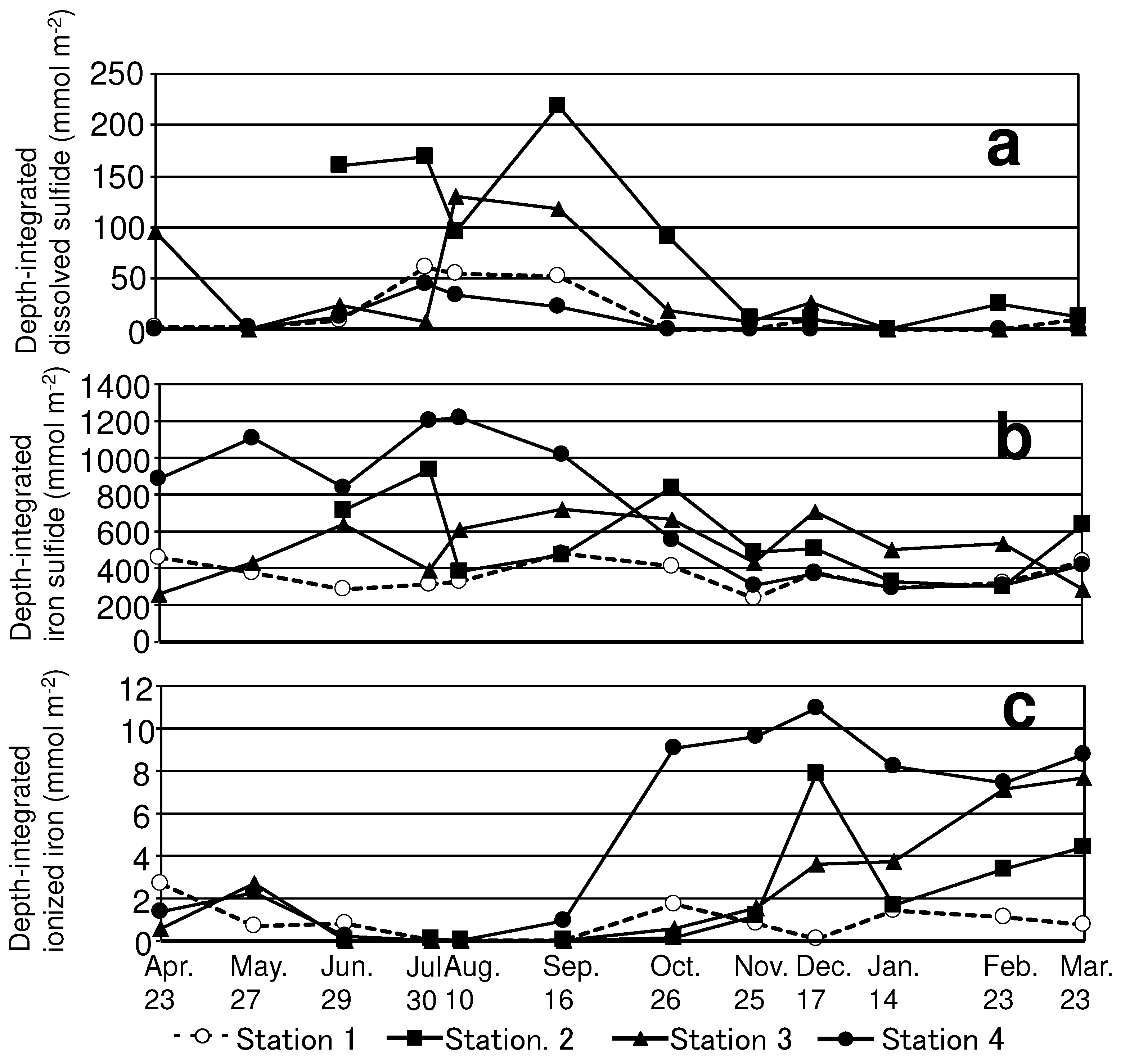
Figure 6 presents representative data showing seasonal changes in depth-integrated dissolved sulfide, iron sulfide, and ionized iron in the upper layer (0-4 cm).
The maximum dissolved sulfide concentrations, integrated from the surface to a depth of 4 cm of sediment for each station, ranged from 44.7 to 219.1 mmol m-2 in summer (Figure 6). Previous studies have reported the release of dissolved sulfide released from anoxic sediments into the water column [11,12,32,33]. The present study shows that part of the dissolved sulfide reaching the surface of the sediment escapes to the water column and acts as an oxygen consumer that sustains anoxic conditions in the bottom water. Dissolved sulfide concentrations were relatively low at Stations 1 and 4, located in the central bay and waterway, respectively, compared to those at Stations 2 and 3 located in the waterway. Waku et al. [10] reported that anoxic conditions of the bottom water were stable for long periods in a waterway associated with a large-scale port, owing to less vertical mixing attributed to its bottom topography, which has a sharp inclination, compared to that of central Mikawa Bay. The relatively high frequency of oxygen supply by temporal vertical mixing accounts for the relatively low concentration of dissolved sulfide at Station 1 in summer. Notably, dissolved sulfide was relatively low at Station 4, despite being located on a waterway. Depth-integrated iron sulfide concentrations in the upper layer of Station 4 were higher (835.2–1220.6 mmol m-2) than those at other stations in summer (Figure 6). The ionized iron concentration in the upper layer of Station 4 increased rapidly to 9.05 mmol m-2 accompanied with the decrease in iron sulfide on October 26. These results suggest that ionized iron (Fe (II)) reacted with dissolved sulfide to form iron sulfide more actively and prevented the enhanced accumulation of dissolved sulfide at Station 4 compared with the other stations. Nevertheless, the maximum concentration of ionized iron was two orders of magnitude lower than that of iron sulfide at Station 4. Despite lacking evidence for the imbalance between the momentary concentration of ionized iron and iron sulfide, the underlying reasons are as follows. Ionized iron (Fe (II)) released by the oxidation of iron sulfide in autumn (Equation (4)) is immediately converted into particulate oxidized iron (FeOOH) (Fossing, 2004.).
4Fe2+ + O2 + 6H2O → 4FeOOH + 8H+
Ionized iron (Fe (II)) released from the particulate oxidized iron by the oxidation of hydrogen sulfide (Equation (6)) and/or by anaerobic bacterial respiration (Equation (7)) [25] in spring, quickly reacted with sulfide to form iron sulfide [30] (Equation (2)).
H2S + 2FeOOH + 4H+ → S0 + 2Fe2+ + 4H2O
4FeOOH + CH2O+ 8H+ → 4Fe2+ + CO2 +7 H2O
As mentioned above, the high turnover rate of ionized iron is considered a reason underlying the low momentary concentration of ionized iron.
4.3. Chemical Buffering Capacity Toward Sulfide
Iron in sediments can potentially react with sulfide, thus preventing the accumulation of free sulfides in the sediment [13,19,20,21,22]. The capacity of the seabed to bind sulfide is called the chemical buffering capacity toward sulfide, the sediment’s hydrogen sulfide buffering capacity, or buffering capacity [25,31].
As mentioned earlier, we observed a seasonal increase/decrease of dissolved sulfide with a decrease/increase of ionized iron in the sediment of the dead zone, where few organisms can survive, which is attributed to severe environmental degradation. This phenomenon was more noticeable at Station 4 compared to the other stations. The Shiokawa River falls into the Shiokawa tidal flat, which is adjacent to Station 4 (Figure 1). A large portion of ionized iron supplied from rivers coagulates and settles in the seabed, accompanied by an increase in salinity [34]. In this study, despite the iron supply mechanism from the river being unknown, the buffering capacity likely depended on the iron supply from the river. We identified the significant role played by iron pools in the prevention of sulfide accumulation in the sediment of the dead zone, where environmental restoration is particularly required.
One more important mechanism of buffering capacity is oxidation reserve, indicating that the iron pools of the seabed can bind sulfide and therefore correspond to oxygen consumption for several months [25]. In other words, iron binds to sulfide within the sediment during summer, causing delayed consumption of oxygen for a few months. In the present study, we observed that iron sulfide precipitated by binding dissolved sulfide and ionized iron rapidly in summer was oxidized during autumn and winter at Station 4 (Figure 6). These results suggest the possibility that artificial addition of sufficient iron compounds to the seabed accelerates the chemical buffering capacity toward sulfide and prevents severe anoxic conditions in the bottom water. Further investigation is needed to assess the iron compound to be added by considering its availability and effectiveness, and to calculate the requisite amount of iron compound via quantitative analyses using numerical models.
5. Conclusions
Dissolved sulfide near the surface increased, with DO depletion at the bottom of the water column in summer at all stations. Depth-integrated dissolved sulfide in the upper layer of sediment was relatively low at the station located near the river compared to other stations located in the waterway associated with a large-scale port. The difference in dissolved sulfide was ascribed to the magnitude of the iron pools in the sediment, which appears to be an important factor in determining the magnitude of dissolved sulfide accumulation in the sediment.
Author Contributions
M. W. designed the study, measured environmental factors, conducted experiments, and drafted the manuscript. R. S. designed the study and measured the environmental factors. T. I. measured environmental factor, and drafted and provided final approval of the manuscript. T. S. designed the study and provided final approval of the manuscript. All the authors have read and agreed to the drafted version of the manuscript.
Funding
This research was supported by the Environment Research and Technology Development Fund of the Ministry of the Environment, Japan (5-1404, Principal Investigator, Prof. Yoshiyuki Nakamura) and jointly conducted by the Aichi Fisheries Research Institute and NIPPON STEEL Corporation research teams.
Acknowledgments
We wish to express our sincere gratitude to Dr. Shogo Sugahara of Shimane University for providing useful information and support. We are grateful to the crew at R/V Heiwa for their cooperation at sea.
Conflicts of Interest
The authors declare no conflicts of interest.
References
- Kodama, K.; Horiguchi, T. Effects of hypoxia on benthic organisms in Tokyo Bay, Japan: A review. Mar. Poll. Bull. 2011, 63, 215–220. [Google Scholar] [CrossRef] [PubMed]
- Sone, R.; Waku, M.; Yamada, S.; Suzuki, T.; Takabe, T. Spatio-temporal dynamics and mortality of mega-benthos in relation to the development of hypoxia in an inner bay : A model study in Mikawa Bay, Japan. Bull. Jpn. Soc. Fish. Oceanogr. 2017, 81, 230–244. [Google Scholar]
- Suzuki, T. Oxygen-deficient waters along the Japanese coast and their effects upon the estuarine ecosystem. J. Environ. Qual. 2001, 30, 291–302. [Google Scholar] [CrossRef] [PubMed]
- Kamohara, S.; Shiba, S.; Tsurushima, D.; Suzuku, T. Relationship of Manila clam (Ruditapes philippinarum) growth with aged changes of total nitrogen and total phosphorus in Mikawa Bay, Japan. Bull. Jpn. Soc. Fish. Oceanogr. 2021, 85, 69–78. [Google Scholar]
- Suzuki, T. Large-scale restoration of tidal flats and shallows to suppress the development of oxygen deficient water masses in Mikawa Bay. Bull. Fish. Res. Agen. 2004, 1, 111–121. [Google Scholar]
- Suzuki, T.; Matsukawa, Y. Hydrography and budget of dissolved total nitrogen and dissolved oxygen in the stratified season in Mikawa Bay, Japan. J. Oceanogr. Soc Jpn. 1987, 43, 37–48. [Google Scholar] [CrossRef]
- Suzuki, T.; Ishii, K.; Imao, K.; Matsukawa, Y. . Box model analysis on phytoplankton production and grazing pressure in a eutrophic estuary. J. Oceanogr. Soc Jpn. 1987, 43, 261–275. [Google Scholar] [CrossRef]
- Waku, M.; Kaneko, K.; Suzuki, T.; Takabe, T. Distribution of dead zones in the coastal waters: A model study in Mikawa Bay, Japan. Bull. Jpn. Soc. Fish. Oceanogr. 2012, 76, 187–196. [Google Scholar]
- Diaz, R. J.; Rosenberg, R. Spreading dead zones and consequences for marine ecosystems. Science 2008, 321, 926–929. [Google Scholar] [CrossRef]
- Waku, M.; Hata, K.; Kaneko, K.; Suzuki, T.; Takabe, T. Adverse effects of dead zones in the coastal waters on the bay-wide material cycle and its remedial measures: An analyze with the ecosystem model in Mikawa Bay, Japan. J. Adv. Mar Sci. Tec. Soc. 2013, 19, 15–27. [Google Scholar]
- Brüchert, V.; Jorgensen, B.B.; Neumann, K.; Riechmann, D.; Schlosser, M.; Schulz, H. Regulation of bacterial sulphate reduction and hydrogen sulphide fluxes in the central Namibian coastal upwelling zone. Geochim. Cosmochim. Ac. 2003, 67, 4505–4518. [Google Scholar] [CrossRef]
- Lavik, G.; Stuhrmann, T.; Brüchert, V.; Van der Plas, A.; Mohrholz, V.; Lam, P.; Mussmann, M.; Fuchs, B. M.; Amann, R.; Lass, U.; Kuypers, M.M.M. Detoxification of sulphidic African shelf waters by blooming chemolithotrophs. Nature 2009, 457, 581–586. [Google Scholar] [CrossRef]
- Canfield, D. E. Reactive iron in marine sediments. Geochim. Cosmochim. Ac. 1989, 53, 619–632. [Google Scholar] [CrossRef]
- Saager, P. M.; De Baar, H. J. W.; Burkill, P. H. Manganese and iron in Indian Ocean waters. Geochim. Cosmochim. Ac. 1989, 53, 2259–2267. [Google Scholar] [CrossRef]
- Canfield, D.E. , Raiswell, R. and Bottrell, S.H.. The reactivity of sedimentary iron minerals toward sulfide. American J. Sci. 1992; 292, 659–583. [Google Scholar]
- Luther Ⅲ, G.W.; Church, T.M.; Scudlark, J.R.; Cosman, C. Inorganic and organic sulfur cycling in salt-marsh pore waters. Science 1986, 232, 746–749. [Google Scholar] [CrossRef]
- Vazquez, F.; Zang, G.J.; Millero, F.J. Effect of metals on the oxidation of H2S in seawater. Geophysical Res. Lett. 1989, 16, 1363–1366. [Google Scholar] [CrossRef]
- Yao, W.; Millero, F.J. . Oxidation of hydrogen sulfide by hydrous Fe(III) oxides in seawater. Mar. Chem. 1996, 52, 1–16. [Google Scholar] [CrossRef]
- Howarth, R.W. Pyrite: Its rapid formation in a salt marsh and its importance in ecosystem metabolism. Science 1979, 203, 49–51. [Google Scholar] [CrossRef]
- Howarth, R.W.; Jørgensen, B.B. Formation of 35S-labelled elemental sulfur and pyrite in coastal marine sediments (Limfjorden and Kysing Fjord, Denmark) during short-term 35SO42− reduction measurements. Geochim. Cosmochim. Ac. 1984, 48, 1807–1818. [Google Scholar] [CrossRef]
- Drobner, E.; Huber, H.; Wächtershäuser, G.; Rose, D.; Stetter, K.O. Pyrite formation linked with hydrogen evolution under anaerobic conditions. Nature 1990, 346, 742–744. [Google Scholar] [CrossRef]
- Stumm, W.; Morgan, J.J. Ch 4.3 Aqueous carbonate system open to the atmosphere. Aquatic chemistry, Wley interscience, New York, 1996; pp 1005.
- Yamamoto, T.; Okai, M.; Takeshita, K.; Hashimoto, T. Characteristics of meteorological conditions in the years of intensive red tide occurrence in Mikawa Bay, Japan. Bull. Jpn. Soc. Fish. Oceanogr. 1997, 61, 114–122. [Google Scholar]
- Sugahara, S.; Suzuki, M.; Kamiya, H.; Yamamuro, M.; Semura, H.; Senga, Y.; Egawa, M.; Seike, Y. Colorimetric determination of sulfide in microsamples. Anal. Sci. 2016, 32, 1129–1131. [Google Scholar] [CrossRef]
- Fossing, H. A model set-up for an oxygen and nutrient flux model for Aarhus Bay (Denmark). NERI Technical Report No. 483. Ministry of the Environment. Denmark 2004; pp.70.
- Middelburg, J.J.; Levin, L.A. Coastal hypoxia and sediment biogeochemistry. Biogeosciences 2009, 6, 1273–1293. [Google Scholar] [CrossRef]
- Canfield, D. E. Factors influencing organic carbon preservation in marine sediments. Chem. Geol. 1994, 114, 315–239. [Google Scholar] [CrossRef]
- Passier, H. F.; Middelburg, J.J.; de Lange, J.J.; Bottcher, M.E. Pyrite contents, microtextures, and sulphur isotopes in relation to formation of the youngest eastern Mediterranean sapropel. Geology 1997, 25, 519–522. [Google Scholar] [CrossRef]
- Taillefert, M.; Bono, A.B.; Luther III, G.W. Reactivity of freshly formed Fe(III) in synthetic solutions and (pore)waters. Voltammetric evidence of an aging process. Environ. Sci. Technol. 2000, 34, 2169–2177. [Google Scholar] [CrossRef]
- Rozan, T. F.; Taillefert, M.; Trouwborst, R.E.; Glazer, B.T.; Ma, S.F.; Herszage, J.; Valdes, L.M.; Price, K.S.; Luther Ⅲ, G. W Iron-sulphur-phosphorus cycling in the sediments of a shallow coastal bay: Implications for sediment nutrient release and benthic macroalgal blooms. Limnol. Oceanogr. 2002, 47, 1346–1354. [Google Scholar] [CrossRef]
- Heijis, S. K.; Jonkers, H.M.; Gemerden, H.V.; Schaub, B.E.M.; Stal, L.J. The buffering capacity towards free sulphide in sediments of a coastal lagoon (Bassin D’ Arcachon, France)-the relative importance of chemical and biological processes. Estuar. Coast. Shelf Sci. 1999, 49, 21–35. [Google Scholar] [CrossRef]
- 32. Mochida, F, Y.; Nakamura, T.; Inoue, H.; Suzuki, T. Reproduction of the suppression effect of iron on sulfide release : verification of the suppression effect of iron. J. Jpn. Soc. Civil. Eng.Ser. G 2021, 77, 241–250.
- Inoue, T.; Hagino, Y. Effects of three iron material treatments on hydrogen sulfide release from anoxic sediments. Water Science and Technology. 2021, 85(1), 305–318. [Google Scholar] [CrossRef] [PubMed]
- Boyle, E.A.; Edmond, J.M.; Sholkovitz, E.R. The mechanism of iron removal in estuaries. Geochim. Cosmochim. Ac. 1977, 41, 1313–1324. [Google Scholar] [CrossRef]
Figure 1.
Study area and location of the observation stations. Solid line and dotted line represent 10 and 5 m isobaths, respectively.
Figure 1.
Study area and location of the observation stations. Solid line and dotted line represent 10 and 5 m isobaths, respectively.
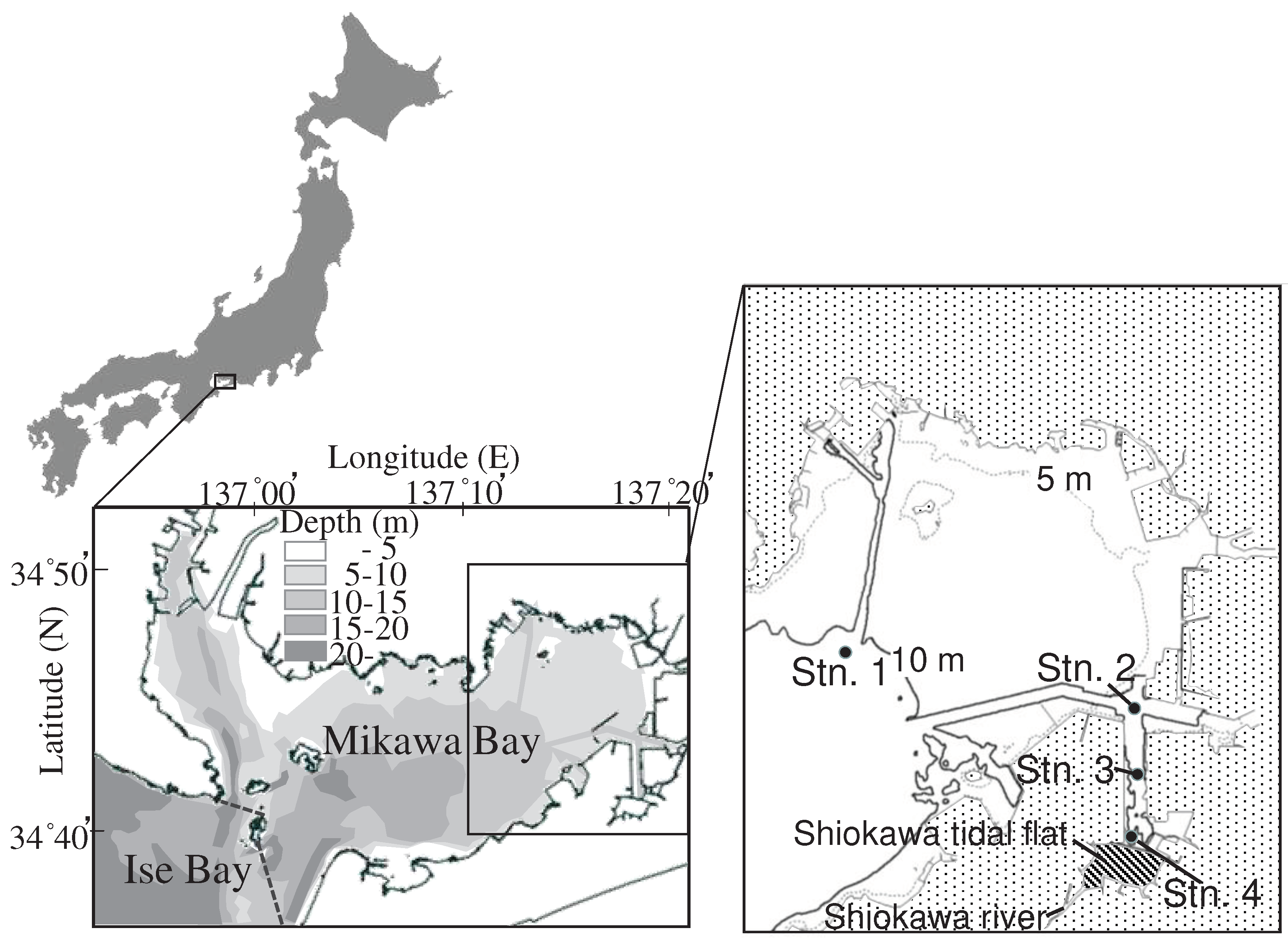
Figure 2.
Vertical profiles of dissolved oxygen (DO) in the water column.
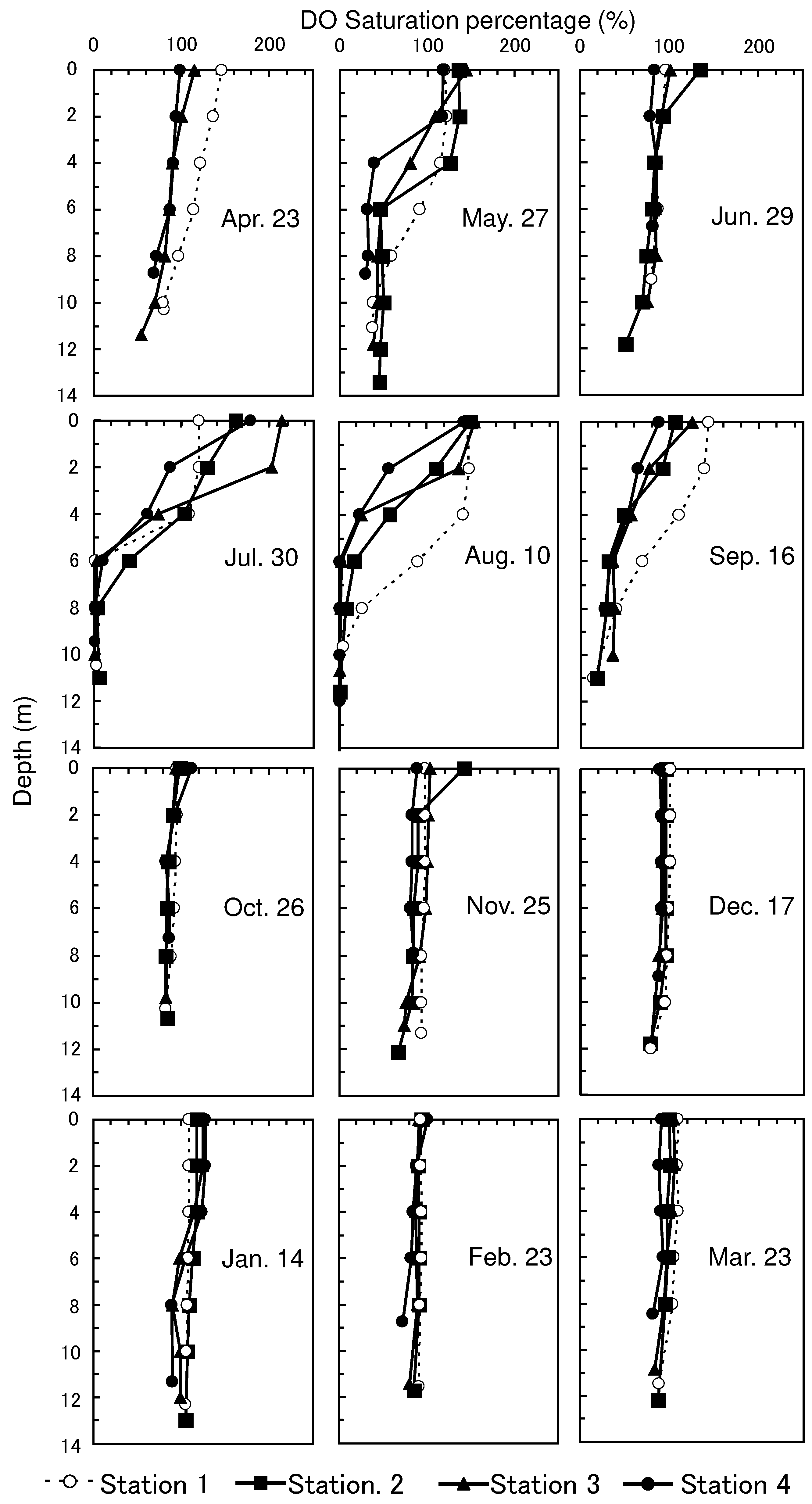
Figure 3.
Vertical profiles of dissolved sulfide in sediment.
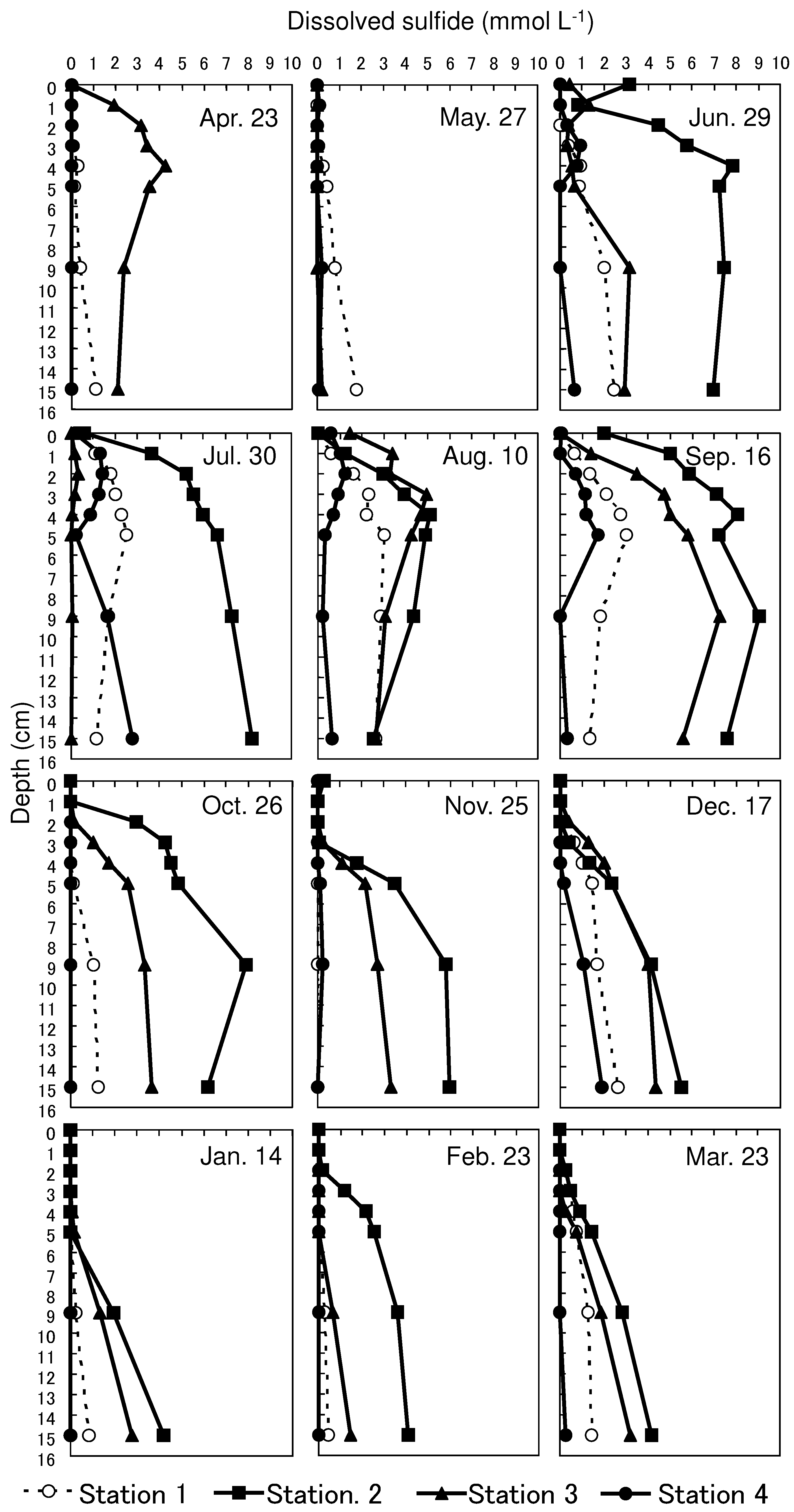
Figure 4.
Vertical profiles of iron sulfide in sediment.
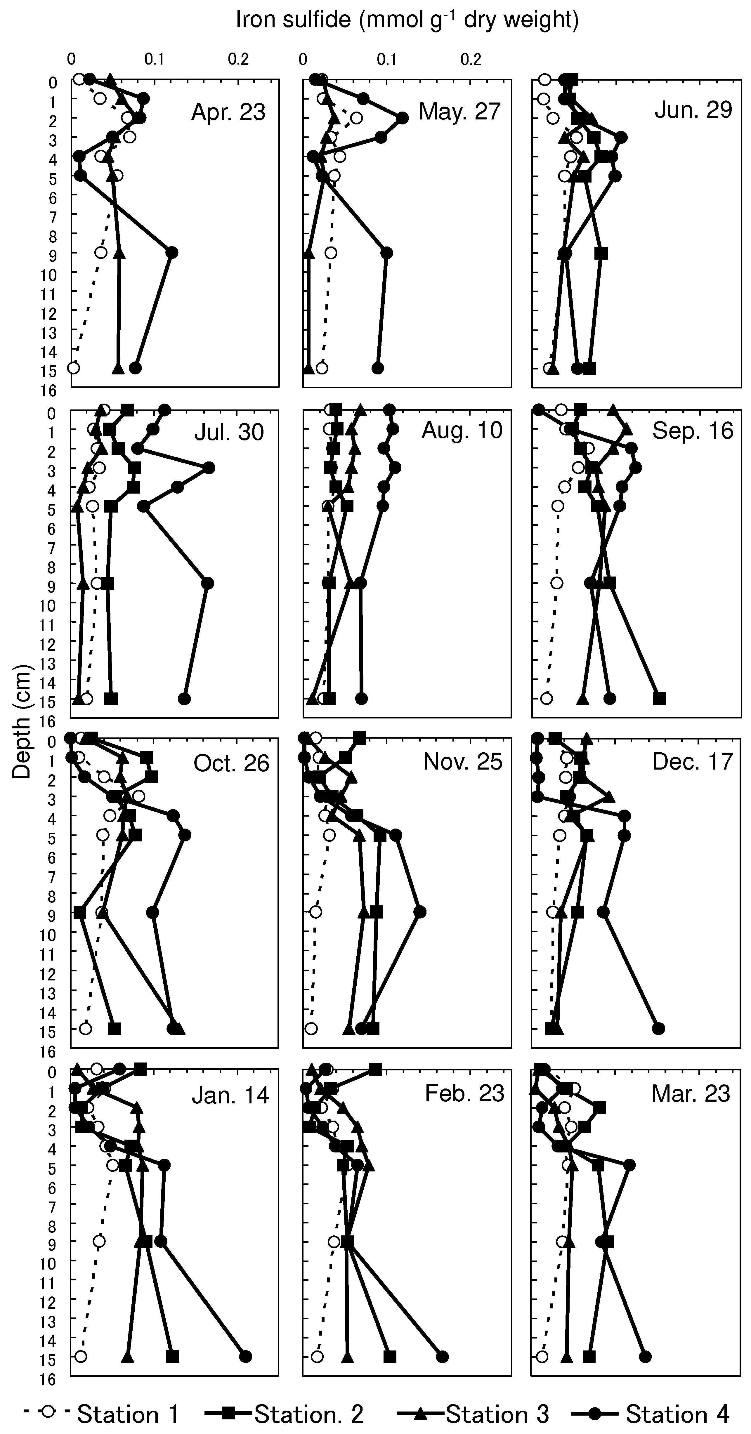
Figure 5.
Vertical profiles of ionized iron in sediment.
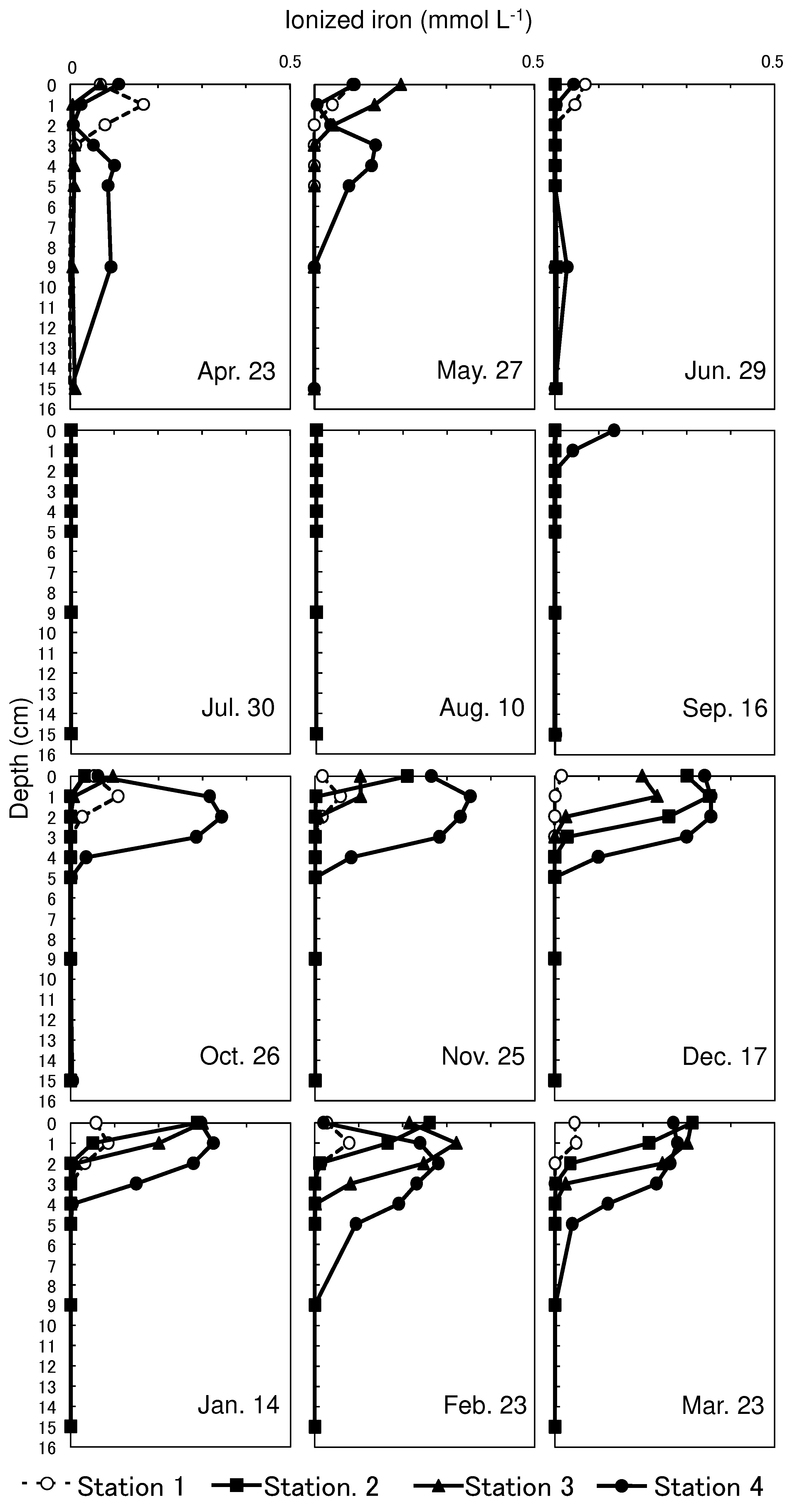
Figure 6.
Seasonal change of depth-integrated dissolved sulfide (a), iron sulfide (b), and ionized iron (c) in the upper 4 cm sediment.
Figure 6.
Seasonal change of depth-integrated dissolved sulfide (a), iron sulfide (b), and ionized iron (c) in the upper 4 cm sediment.
Disclaimer/Publisher’s Note: The statements, opinions and data contained in all publications are solely those of the individual author(s) and contributor(s) and not of MDPI and/or the editor(s). MDPI and/or the editor(s) disclaim responsibility for any injury to people or property resulting from any ideas, methods, instructions or products referred to in the content. |
© 2023 by the authors. Licensee MDPI, Basel, Switzerland. This article is an open access article distributed under the terms and conditions of the Creative Commons Attribution (CC BY) license (http://creativecommons.org/licenses/by/4.0/).
Copyright: This open access article is published under a Creative Commons CC BY 4.0 license, which permit the free download, distribution, and reuse, provided that the author and preprint are cited in any reuse.


