
Submitted:
23 February 2023
Posted:
27 February 2023
You are already at the latest version
Abstract
Climate change in the coming decades could intensify extreme events such as severe droughts. Combined with the possible increase of water demands, these changes exert a large pressure on the water systems. In order to confirm this assumption, a set of scenarios was proposed in this study to consider the combined impact of climate changes and the increase in water demand on the main multiple-use reservoirs of São Francisco River, Brazil. For this purpose, five CMIP6 climate models were used considering two greenhouse gas emissions scenarios: the SSP2-4.5 and SSP5-8.5. The naturalized and withdraw streamflows were estimated to the adopted reser-voirs considering all existing, new and projected demands. The conjunction of scenarios indicat-ed an increase in Potential Evapotranspiration, a possible significant reduction in water availa-bility, a growth in water demand mainly for irrigation and a substantial reduction in the perfor-mance of the evaluated reservoirs.
Keywords:
Climate Change
; Consumptive Demands
; São Francisco River reservoirs.
1. Introduction
Extreme events, such as storms, severe droughts, floods and fires, can be intensified in different regions of the world by climate change in the coming decades, as indicated by several studies that have analyzed possible future scenarios based on greenhouse gas emissions (GEE) with using Global Climate Models (GCM) from the Coupled Model Intercomparison Project (CMIP) project, in a horizon that reaches the year 2100 [1,2].
Regions that already have a history of recurrent and prolonged droughts, such as the Northeast region of Brazil (NEB), may experience this problem even more frequently, with an increase in temperatures between 4° and 5°C, and a possible reduction in rainfall. with percentage anomalies ranging between -20% and 20% in the most pessimistic scenarios in the coming decades [3]. With this, it is possible that the outflows of the main river basins decrease between 60% and 90% [3,4,5].
The São Francisco River is the main water system in the NEB region, being responsible for supplying water for multiple uses (consumer and non-consumer), such as human supply, irrigation, industry, navigation, among others. Among the consumptive uses, irrigation has been the predominant demand in most of the reservoirs that make up the São Francisco River Basin (SFRB) [5].
A project to transfer water from the São Francisco River to the northeastern semi-arid region is currently being completed to reduce vulnerability to droughts and promote regional development. This extra demand will provide water for various purposes, such as human and animal consumption, irrigation, fish, and others, in an area with about 12 million inhabitants [6].
However, this new demand may increase existing water conflicts, especially during extreme events, such as the recent drought from 2012 to 2018, when water supply to urban areas was prioritized according to the federal water resources law (law no. 9,433/97), as well as the production of food with irrigation, to the detriment of hydroelectric power generation, which was reduced from 87.7% in 2011 to 21% in 2017 of the total electricity demand of the region [5].
Such aspects, associated with the possible forecast of increased demand for water in the coming decades, caused by population growth and wealth, may exert great pressure on the region's water systems, significantly influencing the supply of water for various uses.
Faced with this complexity of the water system, one of the challenges is how to evaluate and quantify performance using an approach that captures a variety of uncertainties [7]. One of the most widely used water resources system performance measures is the use of reliability-resilience-vulnerability (RRV) metrics. These metrics were introduced by [8] and complement each other, as each criterion evaluates different aspects of water resource systems [7]. That said, climate change, extreme events, and the impacts on the performance of reservoirs using the RRV have been the subject of several studies [9,10,11].
Among these studies, the work of [9] combine the 3- and 12-month standard precipitation evapotranspiration index (SPEI) and framework RRV to map future river basin health based on the responses of basins across China to different dryness conditions from 2021 to 2050.
Therefore, in this study, a set of scenarios was proposed to consider climate change and the growth of consumption demand, seeking to assess how each demand can increase and its impact on the yield of the reservoirs, through the calculation of indicators, using natural flows of future affluents. While several impacts of climate change on the SFRB have been reported, impacts on reservoir performance due to future climate associated with increased consumption use have not been addressed.
2. Materials and Methods
The methodology was divided in six steps (see Figure 1): i) delimitation of hydrographic basins of the SFRB reservoirs; ii) obtaining projections from CMIP6 models for precipitation and maximum, minimum and average Air Surface Temperature (AST) and estimation of Potential Evapotranspiration (PET); iii) statistical correction of precipitation and ETP projections; iv) calibration and validation of hydrological model SMAP (Soil Moisture Accounting Procedure) for each reservoirs’ watershed; v) obtaining water demands and its projections using ETS (Exponential Smoothing) model; vi) water system operation; vii) water system analysis, determining the occurrence of service failures and the reservoirs yield.
2.1. Coupled Model Intercomparison Project Phase 6
The climate change projections were analyzed with CMIP6 data. These data are provided by simulations of five models: Canadian Earth System Model 5nd generation (CanESM5), Institut Pierre-Simon Laplace-5 Component Models version A-Medium Resolution (IPSL-CM5A-MR), Model for Inter-disciplinary Research on Climate version 6 (MIROC6), Beijing Climate Center-Climate System Model version 2-Medium Resolution (BCC-CSM2-MR), e Meteorological Research Institute Earth System Model Version 2.0 (MRI-ESM2.0). These models are available for download and have projection scenarios. The instructions, countries and papers that discuss the aforementioned models are presented in Table 1.
The CMIP6 has the historical scenario (based on historical observations of the present climate) and future scenarios which combine socioeconomic and technological development, called Shared Socioeconomic Pathways (SSP), with future scenarios of radioactive forcing, called Representative Concentration Pathways (RCP) [17]. In this study, the historical scenario (1971 to 2000, XX century) and the SSP2-4.5 and SSP5-8.5 projection scenarios (2021 to 2050, XXI century) provided monthly time series for precipitation and average, maximum and minimum ATS.
The SSP2 scenario regard a moderate population growth, slower convergence of income levels across countries. In SSP5 a strong global economic growth with the use of fossil fuels and potentially large impacts of climate change is expected [17]. In relation to RCP scenarios, the RCP 4.5 regard stabilization of radiative forcing in 4,5 W/m² before the end of XXI century and the RCP 8.5, the most pessimistic scenery, consider an increasing of radioactive forcing until 2100, reaching 8,5 W/m²[2].
2.2. Observed Data
In this study, the monthly naturalized streamflow series from the National Electric System Operator (ONS, from Portuguese Operador Nacional do Sistema Elétrico) [18] were used for SMAP’s parameters calibration and validate the simulated streamflows. These flows series were obtained for SFRB’s reservoirs and covered the period between 1991 to 2017.
The monthly precipitation series were obtained from pluviometric stations of National Water Agency (ANA, from Portuguese Agência Nacional de Águas) and spatialized using Thiessen method. The monthly PET series were obtained with the Hargreaves-Sammani method [19] using the maximum, minimum and average AST from Climate Research Unit (CRU) [20]. The parameters and initializations of the SMAP model are discussed in the following topics.
2.3. Bias correction
The Gamma Cumulative Distribution Function (Gamma CDF) was adopted to adjust the model's data using the observed data, because the output of the climate models, such as the CMIP6 models, have systemic errors mainly in relation to bias. [5,21]. The Gamma CDF is expressed by the Equation 1:
where x is the variable (in this case, precipitation or PET); β and γ are the scale and shape parameter, respectively; and Γ is the Gamma Function.
The adjustment of the model data was performed on a monthly scale. For this purpose, both modeled and observed time series area fitted to a CDF Gamma, saving the parameters β and γ. Twelve Gamma adjustments were considered, one by each month, i.e., the modeled and observed data were grouped by month and generated the Gamma parameters.
The generated CDF curves allow to check the probabilistic behavior of the model data in relation to the observed data. Thus, to adjust the model data, the probability of the modeled data (precipitation and PET) obtained on its CDF curve are passed as input data to the inverse CDF gamma of the observed data.
2.4. SMAP hydrological model
In this study, the SMAP, a concentrated rainfall-runoff hydrologic model, was used in its monthly version [22]. The SMAP’s monthly version considers two hypothetical reservoirs for water balance: the soil reservoir (Rsolo) and the underground reservoir (Rsub), as shown in Figure 2.
The Monthly SMAP has four parameters: soil saturation capacity (SAT); an exponent related to the surface runoff generation (pes); the aquifer recharge coefficient (Crec), which is related to permeability of the soil’s non-saturated zone; and the constant of recession (K), associated with base flow generation. In addition to these parameters, there are two initialization parameters: the initial soil moisture content , which determines the initial level of the , and the initial base flow . The initialization values and calibrated parameters for each considered reservoir are presented in Table 1.
The level of the two reservoirs ( and ) are update from month to month thought the Equations 2 and 3.
where: is the surface runoff in mm, P is the precipitation (mm) and is the actual evapotranspiration (mm).
The first parameter of the model is the , which, by definition, receives the maximum value of the SAT. In turn, the SAT can be expressed by by equation 4:
The is also calculated using and which is the Potential Evapotranspiration (one of the input variables) through equation 5:
The recharge , which appears in equations 2 and 3, is expressed by equation 6:
The is expressed by equation 7:
The is expressed by equation 8:
The and composes together with the Area, the affluent flow of the basin (Q) in m³/s, given by Equation 9:
In this study, the calibration process was carried out in a single step, in which a set of model parameters (SAT, pes, Crec and K) and initializations were sought that maximize the Nash-Sutcliffe Efficiency Coefficient (NSE) [23] and minimize the Percent Bias (PBIAS) [24]. The NSE and PBIAS are presented in the Equations 10 and 11.
where: is the observed streamflow, is the simulated streamflow, is the average observed streamflow; and n is the number of observation (length of the time series).
The model parameters and initializations obtained in the calibration process are presented in the Table 2 for each of the four considered reservoirs.
2.5. Exponential Smoothing Model and Consumptive Demand Scenarios
The projection of consumptive demands (period from 2018 to 2050) considered four scenarios. In the first scenario, a static demand was adopted, that is, the last withdrawal streamflow was considered for the entire projection period. The second, third and fourth scenarios considered the consumptive demand projected by the ETS model, adopting the average of projected values, the lower bound of the 95% confidence interval and upper bound of the 95% confidence interval, respectively. These projections are performed to three kinds of consumptive water demands: i) human and animal water supply, ii) irrigation and iii) industry.
The ETS model has three components: Error, Trend and Seasonal (E, T, S). The Error component can be Additive (A) or Multiplicative (M); the Seasonal component can be A, M or None (N); the Trend component can be A, M, N, Damped Additive (DA) and Damped Multiplicative (DM). In this study, the ETS model was performed according to [25,26], which is provide in the Forecast Package in R. The choice of the best ETS model was based on Akaike’s Information Criterion (AIC), Schwarz’s Bayesian Information Criterion (BIC) e AIC with bias removed (AICc), expressed in the Equations 14 to 16.
whereby: LL is the log likelihood, Tp is the total of parameters and T is the number of observations.
being the expression the bias correction
where k is the estimate of the model parameters obtained through least squares.
2.6. Information System for Water Allocation Management
The water management of the SFRB was performed through a simulated operation of its hydrosystem using a flow network characterized by different demands and their priorities. The supply guarantees inherent to the permanence curve of their flows were also used. To perform this water management, the Information System for Water Allocation Management (SIGA, from Portuguese Sistema de Informação para o Gerenciamento de Alocação de Água) was employed.
The four multi-purpose reservoirs of the SFRB were modeled in series. In this process, the consumptive water demands and the transposition channels was also considered, forming a network as shown in Figure 3. The North and East axes of the São Francisco River transposition were considered as demands to be met by the system, unifying the different uses, in this case: human, industrial and irrigation. These uses were also modeled in the downstream section of each reservoir in the basin, through the streamflow withdraw for each use.
Besides meeting the water demands, the modeled system also attended to the maximum and minimum streamflow in the river sections, as regulated by the system operator [27]. These limits are presented in Table 3. In this study, the minimum streamflow limits were used.
The network operation simulation is carried out using the equation of the water mass balance in the reservoirs, expressed in Equation 17:
where is the stored volume at the beginning of time step t(hm³); is the stored volume at the beginning of time step t+1 (hm³); is the inflow (natural and transference) volume to the reservoirs during the time step t (hm³); is the evaporated blade during the time step t (hm), which was assumed to be constant over the time step; is the area of the water surface at the beginning time step t, which was assumed constant for small time intervals and a function of (hm²); are the operational withdrawals (hm³); e a is the spill (hm³).
The network simulations had the operational withdrawals optimized to ensure compliance with the operational limits, the maximum meeting of demands and the minimization of the evaporated volume during the simulation periods. This was performed through SIGA® software that use the Multiple Objective Particle Swarm Optimization (MOPSO) as optimization algorithm [28].
During a period when demand is not being met, SIGA® adopts a priority system to determine which nodes in the system will suffer from lack of supply. This priority system considers that the lower the priority value, the higher the priority usage. Table 4 presents the priority system adopted in this study, which prioritizes human supply over irrigation and industry.
The second highest priority value was assigned to the demands of the São Francisco Transposition channels because these waters are used to assist human supply systems in other basins.
2.7. Evaluation of CMIP6 models
The evaluation of CMIP6 models sought to evaluate the ability of these models to represent the seasonality of precipitation in the SFRB watersheds. The Taylor diagram was used [29], allowing to graphically visualize three statistical statistics, these are: Pearson's Correlation Coefficient (r), Standard Deviation (σ) e Root Mean Square Error (RMSE), presented in the Equations 18, 19 e 20, respectively.
where n is the sample space; is the variable observed over time; is the mean of the variable ; is the calculated variable e is the mean of the variable y. For Pearson's correlation coefficient, values of -1 and 1 indicate perfect anticorrelation and perfect correlation, respectively. Also, the value equals zero indicate a complete absence of correlation.
2.8. Hydrological Analysis
2.8.1. Percentual Anomaly
The hydrological analyses consisted in the calculation of the percentual anomaly, expressed by Equation 21:
where is the percentual anomaly, is the average of the variable in the period from 2021 to 2050 in the SSP2-4.5 and SSP5-8.5 scenarios e is the average of the variable in the historical period.
2.8.2. Reliability, Resilience, Vulnerability and Sustainability Indexes
The impacts of low-frequency variability and consumptive demands on reservoir performance were evaluated with the Reliability, Resilience and Vulnerability indexes, proposed by [8].
The Reliability Index (CI) is the probability of the time series remaining in a satisfactory state, that is, the percentage of time the system operates without failure [8]. This index is expressed by Equation 22.
of which: NF is the number of failures and N is the time series length.
Failure occurs when supply is less than demand. Thus, given a demand streamflow and a supply or regularized streamflow
The Resilience Index (RI) is defined by the average ability of the water system to recover from a failed state to a satisfactory state [8]. In this way, it is measured by the inverse of the expected value of the average time that the system remains in failure, and can be calculated by:
where e is the instant of time such that and e is the instant after such that The Vulnerability Index (VI) measures the magnitude of the failure when it occurs. According to [7], the greater the water deficit, the more vulnerable the system will be, and it can be not very resilient but rather vulnerable or the opposite way around. [8] define vulnerability according to Equation 25:
As in the other indexes, the VI had its value multiplied by 100, providing a better analysis and comparison between the indexes.
The Sustainability Index (SI) is directly related to the increase of CI and RI and the decrease of VI, and is defined by Equation 26:
3. Results
3.1. SMAP model Calibration and Validation
Figure 4 shows the calibration (1996 to 2005) and validation (2006 to 2017) results of the simulated streamflows with the SMAP in comparison with ONS’s naturalized streamflows.
According to [30], a hydrological model is considered “very good” if 0.75 <NSE <1.00 e PBIAS < ±10; “good” if 0.60 < NSE ≤ 0.75 e ± 10 < PBIAS ≤ ± 15; “satisfactory” if 0.36 < NSE ≤ 0.60 e ± 15 < PBIAS ≤ ± 25. Thus, it is possible to observe a good performance in most reservoirs. The only exception was the validation period of the Retiro Baixo reservoir which overestimated the ONS naturalized streamflow, showing a PBIAS below satisfactory (-39.7%)
In the Retiro Baixo, Sobradinho and Três Marias reservoirs, the streamflows were also overestimated, presenting negative PBIAS of -19%, -13% and -1%, respectively. In the Itaparica reservoir, the streamflow was underestimated (PBIAS +2.8%). In the validation period, except for Retiro Baixo, the simulated streamflows were underestimated. Regarding the NSE, the Itaparica reservoir had the lowest coefficient both in calibration and validation, being classified as “satisfactory”. In contrast, the Três Marias reservoirs presented the higher NSE, being classified as “very good”
3.2. Perfomance dos modelos do CMIP6
Figure 5 shows the precipitation seasonality of the CMIP6 models compared to the ANA observed precipitation. It can be seen that the bias correction made a good fit of the modeled results with the observed, reflecting the same seasonal behavior.
In the Sobradinho and Itaparica basins, most models overestimated the precipitation in January, February and March, and underestimated in November and December. In the Três Marias basin, most models underestimated the precipitation in all months, except for CanESM5 model, that overestimated the precipitation in January, February and March. In the Retiro Baixo basin, the majority of models overestimated the precipitation in all months, except for CanESM5 model, that underestimated the precipitation in January, February and March.
Figure 6 presents the Taylor Diagram of the precipitation seasonality of the CMIP6 models in relation to observed data. It can be observed that most models exhibited a good performance, with r high than 0.9. Nevertheless, in the watershed located southernmost of the SFRB, the models best represented the seasonality of precipitation, with higher r and lower σ and RMSE. This fact may be related to the greater precipitation variability in the Sobradinho and Itaparica basins, due to the location of these basins in the semiarid region of Brazil. The Brazilian semiarid region is marked by long periods of drought and high rainfall variability.
The CanESM5 model presented r lower that 0.8 and higher σ e RMSE than other models in Sobradinho basin. While in the Itaparica basin, the IPSL-CM6A-LR model had the higher RMSE, above 100. The performance of IPSL-CM6A-LR model reproduced the observed behavior by [4], in which showed that the French model (IPSL-CM6A-LR) was onde of the worst performers in representing the precipitation seasonality in the SFRB between the 27 CMIP5 models.
3.3. Percentual Anomaly
Figure 7 shows the anomalies of PET, precipitation and mean annual streamflow from CMIP6 models under SSP2-4.5 and SSP5-8.5 scenarios (2021 to 2050) compared to the historical scenario (1971 to 2000).
It was observed that all models indicate an increase in PET in both future scenarios and for all analyzed reservoirs. For precipitation, most models indicated a reduction for the Itaparica, Sobradinho and Três Marias watersheds, with values close to -15% in the SSP5-8.5 scenario. The exception was the IPSL-CM6A-LR model, which indicated an increase (close to 5%) in precipitation for the Itaparica basin under SSP5-8.5 scenario.
In Retiro Baixo basin there was uncertainty regarding precipitation in the SSP5-8.5 scenario, with models BCC-CSM2-MR, CanESM5 and IPSL-CM6A-LR indicating am increase, while models MIROC6 and MRI-ESM2-0 indicated a reduction.
For the streamflow, most models pointed to a reduction for Sobradinho and Três Marias watersheds, whit the largest reductions in the SSP5-8.5 scenario. Among these reductions, the CanESM5 model stands out, indicating reductions close to -25% at Sobradinho and close to -40% at Três Marias. For the other reservoirs, the models presented uncertainty regarding the sign and magnitude of the mean annual streamflow anomalies. Finally, it is highlighted the MIROC6 and MIR-ESM2-0 that indicated a reduction in the mean annual streamflow for all reservoirs.
3.4. Consumptive Demands Projections
Figure 8 presents the observed time series of the withdrawal streamflow for consumptive demands (1961 to 2017) as well as the best fit obtained with the ETS model and its projections (2018 to 2050).
For most reservoirs, the ETS (M, M, N) model showed the best fit for irrigation demand, except for Retiro Baixo where the ETS (M, Ad, N) model had the best fit. Furthermore, it was observed that all withdrawal streamflows showed exponential growth in all reservoirs and for all consumptive demands. Among these growths, the demand for irrigation stands out with the largest average annual growth rates: +6.80%, 7.42%, 10.99% and 9.29% for Itaparica, Sobradinho, Três Marias e Retiro Baixo, respectively (see Table 5). It is also the irrigation demand that has the highest total values of withdrawal streamflow in three of the four analyzed reservoirs. The exception was the Retiro Baixo, in which human demand exceeded the others.
The ETS model projected growth scenarios between 2018 to 2050 for most consumptive demands. Two exceptions could be observed in scenario D2 (more optimistic): i) the industry demand that presented a mean annual rate of -3.73%, -0.70%, -0.08% and -1.53% for the Itaparica, Sobradinho, Três Marias and Retiro Baixo reservoirs, respectively; and ii) human supply demand that showed a mean annual rate of -1.02% for the Três Marias reservoir.
3.5. Reliability, Resilience, Vulnerability and Sustainability Indexes
Figure 9 presents the Reliability index for the Itaparica, Sobradinho, Três Marias and Retiro Baixo reservoir under scenarios of climate change and consumptive demands projections. For all models, climate change scenarios and almost all consumptive demand scenarios, except for scenario D1, a decrease in the Reliability index was observed for at least one consumptive demand, indicating failure or increase in failures for the next decades (2021 to 2050) in every analyzed reservoir.
For Itaparica reservoir, the Reliability Index was lower in the most pessimistic scenarios. For example, it ranged from 100% in the historical and D1/SSP2-4.5 scenarios to 79% in the D2/SSP5-8.5 scenario for human supply demand. For Irrigation demand, this index varied from 100% in the historical and D1/SSP2-4.5 scenarios to 80% in the D3/SSP5-8.5 scenario. For Industry demand, the reduction was from 100% (historical and D1/SSP2-4.5 scenarios) from 75% (D4/SSP5-8.5 scenario).
For Sobradinho reservoir, the Reliability index has decreased for human supply demand, varying from 100% in the historical and D1/SSP2-4.5 scenarios from 83% in the D4/SSP5-8.5 scenario. For industry demand, in the same reservoir, this index range from 100% (historical and D1/SSP2-4.5 scenarios) to 82% in the D3/SSP2-4.5 and D3/SSP5-8.5 scenarios. For the irrigation demand, no failures were observed on the historical period and all analyzed scenarios, thus, a Reliability index of 100%.
The Retiro Baixo reservoir was the only reservoir analyzed that has failures in the historical period, presenting a Reliability index equal to 0% for the irrigation and industry demands in the historical period and in all analyzed scenarios. These results coincide with those obtained in the studies of [5,31]. For human supply demand, there was a reduction from 100% in the historical and D1/SSP2-4.5 scenarios to 0% in the D4/SSP5-8.5 scenario.
In the Três Marias reservoir there was also a decrease in the Reliability indexes for all analyzed demands. In the historical period and D1/SSP2-4.5 scenario, this reservoir presented a Reliability Index of 100% for all analyzed demands. However, it showed a Reliability Index of 80% for human supply demand in the D2/SSP2-4.5 and D2/SSP5-8.5 scenarios. For the irrigation demand, the lowest Reliability index was equal to 85% in the D2/SSP5-8.5 scenario. For the industry demand, the lower index was equal to 75% in the D2/SSP2-4.5 and D2/SSP5-8.5 scenarios.
Figure 10 presents the Resilience index for the Itaparica, Sobradinho, Três Marias and Retiro Baixo reservoir under scenarios of climate change and consumptive demands projections. This index showed a lower capacity to recover after failure in the evaluated reservoirs, the more pessimistic the projection scenario for the next decades (2021 to 2050) is.
In the Sobradinho reservoir, the Resilience Index ranged from 100% in the historical period to 84% in the D4/SSP2-4.5 and D4/SSP5-8.5 scenarios for human supply demand. For the irrigation demand, this index varied from 100% in the historical period to 82% in the D4/SSP5-8.5 scenario. The Resilience Index for industry demand in this same reservoir presented the largest decrease: from 100% in the historical period to 67% in the D3/SSP2-4.5 scenario.
The Resilience index of the Retiro Baixo reservoir, as well as the Reliability index, was equal to 0% in the historical period and all analyzed scenarios. For the human supply demand, this index decreased according the most pessimistic scenarios, presenting a value equal to 0% in the D4/SSP2-4.5 and D4/SSP5-8.5 scenarios.
The Resilience index of the Três Marias reservoir varied from 100% in the historical period and D1/SSP2-4.5 and D1/SSP5-8.5 scenarios to 72% in the D2/SSP2-4.5 and SSP5-8.5 scenarios. The irrigation and industry demands decreased from 100% in the historical period and D1/SSP2-4.5 and D1/SSP5-8.5 scenarios to, respectively, 79% in the D2/SSP2-4.5 and D2/SSP5-8.5 scenarios and 70% in the D3/SSP2-4.5 scenario.
Figure 11 presents the Vulnerability index for all analyzed reservoirs and consumptive demands for the historical period (1971 to 2000) and for the scenarios of climate change and consumptive demands projections (2021 to 2050).
In the Três Marias reservoir, the vulnerability index was equal to 0% in the historical period and in all scenarios of consumptive demands and climate change for all analyzed models. This behavior demonstrates a low severity in the failures presented during the water system simulation.
The Sobradinho reservoir also presented a Vulnerability index equal to 0% in the historical period and in most projection scenarios and used models, except for MIR-ESM2-0 model that presented a Vulnerability index equal to 100% for the irrigation and industry demands in the D3/SSP5-8.5 and D4/SSP5-8.5 scenarios, which resulted in an average value equal to 20%.
In contrast to the above-mentioned reservoirs, the Retiro Baixo and Itaparica reservoirs presented the highest vulnerability indexes, indicating high severity in the failures during the water systems simulation.
The Retiro Baixo reservoir presented in the historical period a Vulnerability index equal to 0% for human supply demand and 100% for irrigation and industrial demands. Under the scenarios of climate change and consumptive demand projections, the Vulnerability index increased considerably, reaching 74% in the D4/SSP5-8.5 scenario, i.e., there was an increase in the failure severity for this demand.
The Itaparica reservoir presented a Vulnerability index of 0% in the historical period for all analyzed demands, increasing in the scenarios of consumptive demands and climate change. The highest Vulnerability index for human supply demand was 60% in the D3/SSP2-4.5 scenario. For irrigation demand, the largest index occurred in the D4/SSP2-4.5 and D4/SSP5-8.5 scenarios. For industry demand, the biggest index occurred in the following scenarios: D3/SSP2-4.5, D4/SSP2-4.5 and D4/SSP5-8.5.
Figure 12 presents the Sustainability Index (SI) for all analyzed reservoirs and consumptive demands for the historical period (1971 to 2000) and for the scenarios of climate change and consumptive demands projections (2021 to 2050). As already mentioned, this index considers the indexes previously analyzed, reflecting the fulfillment of demands and the frequency, magnitude, and duration of failures in meeting them. The result showed a decrease in SI for all evaluated reservoirs under climate change and consumptive demands projections scenarios.
In the Itaparica reservoir, the SI for human supply demand was 100% in both historical period and D1/SSP2-4.5 scenario, reaching the lowest value of 54% in the D2/SSP2-4.5 scenario. For irrigation demand, the SI presented an average value of 100% only in the historical period, with the lowest average value (51%) in the D4/SSP2-4.5 and D4/SSP5-8.5. For the industry demand, the SI also showed the value of 100% in the historical period, with the lowest value of 41% in the D4/SSP2-4.5 and D4/SSP5-8.5 scenarios.
In the Retiro Baixo reservoir, the SI, as well as the other indexes, presented a value of 0% for irrigation and industry demands in the historical period and in all analyzed scenarios. For the human supply demand, the index value decreases with the most pessimistic scenarios, showing a value fo 0% in most projection scenarios, except for D1/SSP2-4.5 and D1/SSP5-8.5 scenarios which showed 40% and 17%, respectively.
In the Sobradinho reservoir, the SI showed a value of 100% in the historical period and D1/SSP2-4.5 and D1/SSP5-8.5 scenarios for all consumptive demands. The lowest value of SI for irrigation and human supply demands occurred in the D4/SSP5-8.5, with values of 70% and 22%, respectively. For industry demand, the lowest SI value (55%) occurred in scenarios D3/SSP2-4.5 and D3/SSP5-8.5.
In the Três Marias reservoirs, the SI presented a value of 100% in the historical period and D1/SSP2-4.5 and D1/SSP5-8.5 scenarios for all consumptive demands. In the D2/SSP2-4.5 scenario, the SI reached to the lowest value for irrigation and human supply demand equal to, respectively, 58% and 68%. For the industry demand, the lowest value occurred in the D3/SSP2-4.5 scenario with a value of 47%.
4. Discussion
In this study, the outflows of the reservoirs were estimated using the SMAP model, a process that included a calibration period (1996 to 2005) and validation (2006 to 2017). In this process, it was observed that most of the reservoirs presented good performance according to the classification presented in the study by [30], which uses NSE and PBIAS as metrics. The exception was in the validation period of the Retiro Baixo reservoir, which presented a PBIAS equal to 39.7%, a period in which the SMAP model overestimated the naturalized flows of the ONS with a metric below what is considered satisfactory.
The results with NSE for calibration were close to those obtained in the study by [5], which used different periods in each reservoir: Sobradinho (1998 to 2005) with NSE of 0.90; Itaparica (1983 to 1990) with NSE of 0.36; Três Marias (1971 to 1978) with NSE of 0.90; and Retiro Baixo (1986 to 1993) with NSE of 0.86.
In this study and in the work of [5] the Itaparica reservoir was the one that presented the lowest NSE value, obtaining only satisfactory classification. This may be related to the high variability of rainfall and flows in the region, as mentioned in several studies [32,33,34].
Regarding the CMIP6 models, a performance test was carried out, which showed that the models are efficient in representing the seasonality of precipitation over the SFRB. These results coincide with those presented by [35,36] who evaluated the performance of 46 and 50 CMIP6 models, respectively, over South America and the southern regions of the Amazon and southeastern Brazil. Among the evaluated models, the five models used in this study showed good performance. Even the IPSL-CM6A-LR model stood out as one of the models with the best performance in simulating seasonal precipitation over the SFRB, according to [35].
This result demonstrates that the IPSL-CM6A-LR model showed a great improvement in relation to its previous version, the IPSL-CM5A-LR of CMIP5. Because in the study by [4], which evaluated the performance of the CMIP5 models in representing seasonal precipitation over the SFRB, the French model was one of those that presented the worst performance.
This improvement of the IPSL-CM6A-LR model in relation to its previous version was the subject of study in [13]. It showed the different components of the model, their coupling and the simulated weather compared to previous versions. Equilibrium weather sensitivity and transient weather response increased. On the other hand, although they have been reduced, several known biases and shortcomings, for example, dual Intertropical Convergence Zone (ITCZ) frequency of mid-latitude winter locks and El Niño–Southern Oscillation [ENSO] dynamics persist in the current version of CMIP6. This condition may explain the greater deviation for the Itaparica reservoir, where seasonal variability is more sensitive to these phenomena, especially ENSO.
For the climate projections for the SSP2-4.5 and SSP5-8.5 scenarios, the CMIP6 models indicated an increase in PET for all analyzed reservoirs. For precipitation the models indicated uncertainties with the BCC-CSM2-MR, CanESM5 and IPSL-CM6A-LR models indicating an increase, while the MIROC6 and MRI-ESM2-0 models indicated a decrease in precipitation. For flow, most CMIP6 models indicated a reduction for the Itaparica, Sobradinho and Três Marias reservoirs, with a magnitude between -25% and -40% for the SSP5-8.5 scenario. These results are close to those obtained in the studies by [3,4,37], which used the CMIP5 models.
Among these works that used the CMIP5 models, the work of [4] showed that the models differ regarding the future of precipitation for both scenarios. However, they agree that the temperature should increase in the period from 2011 to 2100, disagreeing only in magnitude. For the RCP8.5 scenario, the impacts on temperature are greater, especially in the last 30 years of the 21st century, where the temperature anomaly is greater than 4°C for most models.
Hence, similar results among the CMIP5 and CMIP6 databases show the cohesion in the methodologies adopted for the projection of climate variables. This way, recent studies like this one end up contributing to the confirmation of results obtained in previous studies, respecting the uncertainties associated with the process.
Added to these results, the projections of consumptive demands indicated a significant increase. The exceptions were the demands of the industry which, in the D2 scenario (more optimistic), projected a reduction in the outflows withdrawn with an average annual rate of 3.73%, 0.70%, 0.08% and 1.53% for the reservoirs of Itaparica, Sobradinho, Três Marias and Retiro Baixo, respectively, and human consumption with an average annual rate of 1.02% for the Três Marias reservoir. These results were the same obtained in the study by [5], as the same methodology was used. However, only this study and that of [5] considered the increase in consumptive demands for studies involving water and energy security, respectively.
In the study by [31], for example, he used fixed consumptive demands for the operation of the hydroelectric system at SFRB to verify the influence of low frequency phenomena on hydroelectric power generation. He claims that it was a limitation to use fixed demands, as the results of the impacts may have been smoothed. The study by [38], for example, has already demonstrated the possible increase in irrigation through the expansion of local agriculture in the SFRB for the next two decades, which may intensify disputes over water in the basin. This result coincides with those obtained with the projections with the ETS model in this study and in the study by [5].
With the projections of consumptive demands and climate changes in the coming decades, this study evaluated SFRB's performance in meeting consumptive demands with the operation of the water system in accordance with law 9,433, which prioritizes human consumption to the detriment of other consumptions. Performance was measured using the RRV.
The results showed a decrease in the Reliability index in most of the analyzed reservoirs, which indicates an increase in service failures. The exception was the irrigation demand for the Sobradinho reservoir.
In addition, except for the Retiro Baixo reservoir, which presented a 0% Reliability index from the historical scenario for the demands of Irrigation and Industry, the other reservoirs only showed a decrease in the Reliability index in the joint scenarios of Climate Change and increase in consumptive demands. This result demonstrates that Climate Change is not enough to identify possible impacts on reservoir performance, since the increase in consumptive demands is notorious.
For the Resilience index, the results were similar, with a significant decrease in the joint climate change scenarios and an increase in consumptive demands, demonstrating that the reservoirs had greater difficulty in recovering after a failure.
In addition, the Vulnerability index increased, indicating that the magnitude of failures may increase with climate change scenarios and increased consumptive demands. With the increase of failures, their magnitude and increase in recovery time after a failure, the Sustainability index decreased for all analyzed reservoirs.
5. Conclusions
In this work a set of scenarios was analyzed to consider climate change and the growth of consumptive demands, seeking to evaluate how the changes in hydrological variables and consumptive demands impact the performance of the Sobradinho, Itaparica, Retiro Baixo and Três Marias reservoirs, in the SFRB. For this purpose, the Reliability, Resilience, Vulnerability, and Sustainability indexes were used.
Climate Change scenarios indicated an increase of PET for all analyzed reservoirs. On the other hand, most climate models pointed out to a reduction in precipitation for Itaparica, Sobradinho and Três Marias reservoirs, with the largest reduction close to -15% in the SSP5-8.5 scenario. In the Retiro Baixo reservoir, there was uncertainty about the precipitation behavior because the models BCC-CSM2-MR, CanESM5 and IPSL-CM6A-LR indicated an increase and the models MIROC6 and MRI-ESM2-0 pointed to a reduction.
In addition to these results, the ETS model projected growth scenarios for most consumptive demands for the period from 2018 to 2050. An exception was the industry demand on the Itaparica, Sobradinho, Três Marias and Retiro Baixo, which scenario D2 (mosto optimistic) projected a reduction of the withdrawn flows with an average annual rate of 3.73%, 0.70%, 0.08% e 1.53%, respectively. Another exception was the human supply demand for the Três Marias reservoir, which projected a reduction with an average annual rate of 1.02%.
Regarding the performance of the reservoirs, from the results presented in this study, it was possible to verify significant impacts in meeting the consumptive demands. Because there was a decrease in the Reliability index, due to the increase in the number of service failures; decrease in the Resilience index, due to the increase in recovery time after a service failure; and an increase in the Vulnerability index, due to the increase in the severity of service failure. According to this set of measures, the studied reservoirs obtained a worrying classification, presenting a low indicator of hydrological sustainability.
In view of this, specific solutions may include more efficient water distribution and irrigation techniques, sewage treatment for agricultural use, switching to crops that are more resilient to drought induced by climate change, education on water use, reforestation and revegetation of zones riparian zones and reforestation in spring areas.
Additional research may consider different scenarios of natural and anthropic land use, verifying their impacts and possible specific solutions mentioned above. In the study of [39] as a result, it was possible to detect an anthropic modification of SFRB, which is the main component of its streamflow variation, in addition to increased streamflow sensitivity to climate variations. Demonstrating it is essential that the territorial planning of the basin be incorporated into the management of water resources. This planning is mainly based on understanding the impacts of those changes on the hydrological processes of the basin. Its main function is to guide actions to preserve the basin and mitigate those impacts, ensuring the protection of this resource for current and future generations.
Author Contributions
Conceptualization, methodology and validation, M.V.M.d.S. and C.d.S.S.; software, M.V.M.d.S; formal analysis, investigation, resources, data curation, M.V.M.d.S.; writing—original draft preparation, M.V.M.d.S., C.E.S.L and C.d.S.S.; writing—review and editing, visualization and supervision, C.d.S.S. and C.E.S.L. All authors have read and agreed to the published version of the manuscript.
Funding
This research was funded by Fundação Cearense de Apoio ao Desenvolvimento Científico e Tecnológico (FUNCAP) (grant number 001), and the Conselho Nacional de Desenvolvimento Científico e Tecnológico -Brasil (Uma análise sobre nexo: Clima, água e energia na bacia do rio São Francisco Project, No. 310286/2018-2).
Data Availability Statement
The study did not report any data.
Acknowledgments
The authors thank the Search Group “Gerenciamento do Risco Climático para a Sustentabilidade Hídrica” of Federal University of Ceará coordinated by Francisco de Assis de Souza Filho.
Conflicts of Interest
“The authors declare no conflict of interest.”
References
- IPCC Summary for Policymakers: Climate Change 2022_ Impacts, Adaptation and Vulnerability_Working Group II contribution to the Sixth Assessment Report of the Intergovernamental Panel on Climate Change; 2022; ISBN 9781009325844. 10.1017/9781009325844.Front.
- IPCC Summary for policymakers. Manag. Risks Extrem. Events Disasters to Adv. Clim. Chang. Adapt. Spec. Rep. Intergov. Panel Clim. Chang. 2014, 9781107025, 3–22.
- Jong, P.; Tanajura, C.A.S.; Sánchez, A.S.; Dargaville, R.; Kiperstok, A.; Torres, E.A. Hydroelectric production from Brazil’s São Francisco River could cease due to climate change and inter-annual variability. Sci. Total Environ. 2018, 634, 1540–1553. [Google Scholar] [CrossRef] [PubMed]
- Silveira, C. da S.; Filho, F. de A. de S.; Martins, E.S.P.R.; Oliveira, J.L.; Costa, A.C.; Nobrega, M.T.; de Souza, S.A.; Silva, R.F.V. Mudanças climáticas na bacia do rio São Francisco: Uma análise para precipitação e temperatura. Rev. Bras. Recur. Hidricos 2016, 21, 416–428. [Google Scholar]
- Silva, M.V.M.; Silveira, C. da S.; Costa, J.M.F. da; Martins, E.S.P.R.; Vasconcelos Júnior, F. das C. Projection of Climate Change and Consumptive Demands Projections Impacts on Hydropower Generation in the São Francisco River Basin, Brazil. Water 2021, 13, 332–10. [Google Scholar] [CrossRef]
- BRASIL Projeto de Integração do São Francisco. Available online: https://antigo.mdr.gov.br/images/stories/ProjetoRioSaoFrancisco/ArquivosPDF/documentostecnicos/RIMAJULHO2004.pdf (accessed on Mar 25, 2021).
- Asefa, T.; Clayton, J.; Adams, A.; Anderson, D. Performance evaluation of a water resources system under varying climatic conditions: Reliability, Resilience, Vulnerability and beyond. J. Hydrol. 2014, 508, 53–65. [Google Scholar] [CrossRef]
- Hashimoto, T.; Stedinger, J.R.; Loucks, D.P. Reliability, resiliency, and vulnerability criteria for water resource system performance evaluation. Water Resour. Res. 1982, 18, 14–20. [Google Scholar] [CrossRef]
- Zeng, P.; Sun, F.; Liu, Y.; Che, Y. Future river basin health assessment through reliability-resilience-vulnerability: Thresholds of multiple dryness conditions. Sci. Total Environ. 2020, 741, 140395–10. [Google Scholar] [CrossRef] [PubMed]
- Sung, J.H.; Chung, E.S.; Shahid, S. Reliability-Resiliency-Vulnerability approach for drought analysis in South Korea using 28 GCMs. Sustain. 2018, 10. [Google Scholar] [CrossRef]
- Bhere, S.; Reddy, M.J. Assessment of Reliability, Resilience, and Vulnerability (RRV) of terrestrial water storage using Gravity Recovery and Climate Experiment (GRACE) for Indian river basins. Remote Sens. Appl. Soc. Environ. 2022, 28, 100851–10. [Google Scholar] [CrossRef]
- Swart, N.C.; Cole, J.N.S.; Kharin, V. V.; Lazare, M.; Scinocca, J.F.; Gillett, N.P.; Anstey, J.; Arora, V.; Christian, J.R.; Hanna, S.; et al. The Canadian Earth System Model version 5 (CanESM5.0.3). Geosci. Model Dev. 2019, 12, 4823–4873. [Google Scholar] [CrossRef]
- Boucher, O.; Servonnat, J.; Albright, A.L.; Aumont, O.; Balkanski, Y.; Bastrikov, V.; Bekki, S.; Bonnet, R.; Bony, S.; Bopp, L.; et al. Presentation and Evaluation of the IPSL-CM6A-LR Climate Model. J. Adv. Model. Earth Syst. 2020, 12, 1–52. [Google Scholar] [CrossRef]
- Hirota, N.; Ogura, T.; Tatebe, H.; Shiogama, H.; Kimoto, M.; Watanabe, M. Roles of shallow convective moistening in the eastward propagation of the MJO in MIROC6. J. Clim. 2018, 31, 3033–3047. [Google Scholar] [CrossRef]
- Wu, T.; Lu, Y.; Fang, Y.; Xin, X.; Li, L.; Li, W.; Jie, W.; Zhang, J.; Liu, Y.; Zhang, L.; et al. The Beijing Climate Center Climate System Model (BCC-CSM): The main progress from CMIP5 to CMIP6. Geosci. Model Dev. 2019, 12, 1573–1600. [Google Scholar] [CrossRef]
- Yukimoto, S.; Kawai, H.; Koshiro, T.; Oshima, N.; Yoshida, K.; Urakawa, S.; Tsujino, H.; Deushi, M.; Tanaka, T.; Hosaka, M.; et al. The meteorological research institute Earth system model version 2.0, MRI-ESM2.0: Description and basic evaluation of the physical component. J. Meteorol. Soc. Japan 2019, 97, 931–965. [Google Scholar] [CrossRef]
- Gidden, M.J.; Riahi, K.; Smith, S.J.; Fujimori, S.; Luderer, G.; Kriegler, E.; Van Vuuren, D.P.; Van Den Berg, M.; Feng, L.; Klein, D.; et al. Global emissions pathways under different socioeconomic scenarios for use in CMIP6: A dataset of harmonized emissions trajectories through the end of the century. Geosci. Model Dev. 2019, 12, 1443–1475. [Google Scholar] [CrossRef]
- ONS Plano de Operação Energética 2019-2023. Available online: http://www.ons.org.br/AcervoDigitalDocumentosEPublicacoes/PEN_Executivo_2019-2023.pdf.
- Hargreaves, G.H.; Samani, Z.A. Reference Crop Evapotranspiration from Temperature. Appl. Eng. Agric. 1985, 1, 96–99. [Google Scholar] [CrossRef]
- Harris, I.; Osborn, T.J.; Jones, P.; Lister, D. Version 4 of the CRU TS monthly high-resolution gridded multivariate climate dataset. Sci. Data 2020, 7, 1–18. [Google Scholar] [CrossRef] [PubMed]
- Silveira, C. da S.; de Souza Filho, F. de A.; Vasconcelos Júnior, F. das C. Streamflow projections for the Brazilian hydropower sector from RCP scenarios. J. Water Clim. Chang. 2017, 8, 114–126. [Google Scholar] [CrossRef]
- Lopes, J.E.G.; Braga, B.P.F.; Conejo, J.G.L. SMAP - A Simplifi ed Hydrological Model, Applied Modelling in Catchment Hydrology. Water Resourses Publ. 1982. [Google Scholar]
- Nash, J.E.; Sutcliffe, J. V. River flow forecasting through conceptual models part I - A discussion of principles. J. Hydrol. 1970, 10, 282–290. [Google Scholar] [CrossRef]
- Gupta, H.V.; Sorooshian, S.; Yapo, P.O. Status of Automatic Calibration for Hydrologic Models: Comparison with Multilevel Expert Calibration. J. Hydrol. Eng. 1999, 4, 135–143. [Google Scholar] [CrossRef]
- Hyndman, R.J.; Koehler, A.B.; Snyder, R.D.; Grose, S. A state space framework for automatic forecasting using. Int. J. Forecast. 2002, 18, 439–454. [Google Scholar] [CrossRef]
- Hyndman, R.J.; Akram, M.; Archibald, B.C. The admissible parameter space for exponential smoothing models. Ann. Inst. Stat. Math. 2008, 60, 407–426. [Google Scholar] [CrossRef]
- ONS Submódulo 23.5: Critérios para estudos hidrológicos; 2011. 2011.
- Sugawara, E.; Nikaido, H. Properties of AdeABC and AdeIJK efflux systems of Acinetobacter baumannii compared with those of the AcrAB-TolC system of Escherichia coli. Antimicrob. Agents Chemother. 2014, 58, 7250–7257. [Google Scholar] [CrossRef]
- Taylor, K.E. Summarizing multiple aspects of model perfomance in a single diagram. J. Geophys. Res. Atmos. 2001, 106, 7183–7192. [Google Scholar] [CrossRef]
- Almeida, R.A.; Pereira, S.B.; Pinto, D.B.F. Calibration and validation of the SWAT hydrological model for the Mucuri river basin. Eng. Agric. 2018, 38, 55–63. [Google Scholar] [CrossRef]
- Ferreira da Costa, J.M.; Silveira, C.S.; Vasconcelos Júnior, F. das C.; Marcos Junior, A.D.; da Silva, M.V.M.; Ramos, S.F.C.; Porto, V.C.; Souza Filho, F. de A.; Martins, E.S.P.R. The water, climate and energy nexus in the São Francisco River Basin, Brazil: an analysis of decadal climate variability. Hydrol. Sci. J. 2022, 67, 1–20. [Google Scholar] [CrossRef]
- Hounsou-Gbo, G.A.; Araujo, M.; Bourlès, B.; Veleda, D.; Servain, J. Tropical Atlantic contributions to strong rainfall variability along the northeast Brazilian coast. Adv. Meteorol. 2015, 2015. [Google Scholar] [CrossRef]
- Fetter, R.; de Oliveira, C.H.; Steinke, E.T. Proposition of an index for the study of the variability of space-temporal rainfall in Brazil. Rev. Bras. Meteorol. 2018, 33, 225–237. [Google Scholar] [CrossRef]
- Paulo, V.D.E.; Da, R.; Ricardo, E.; Pereira, R.; Silveira, R.; Almeida, R. ESTUDO DA VARIABILIDADE ANUAL E INTRA-ANUAL DA PRECIPITAÇÃO NA REGIÃO NORDESTE DO BRASIL Universidade Federal de Campina Grande, Unidade Acadêmica Ciências Atmosféricas, Campina Grande, Universidade Estadual da Paraíba, Campina Grande, PB, Brasil Re. 2012, 163–172.
- Dias, C.G.; Reboita, M.S. Assessment of CMIP6 Simulations over Tropical South America. Rev. Bras. Geogr. Física 2021, 03, 1282–1295. [Google Scholar] [CrossRef]
- de Oliveira, D.M.; Ribeiro, J.G.M.; de Faria, L.F.; Reboita, M.S. Performance of CMIP6 climate models in simulating precipitation in subdomains of South America in the historical period. Rev. Bras. Geogr. Fis. 2023, 16, 116–133. [Google Scholar]
- Silveira, C. da S.; Filho, F. de A. de S.; Costa, A.A.; Cabral, S.L. Performance assessment of CMIP5 models concerning the representation of precipitation variation patterns in the twentieth century on the northeast of Brazil, Amazon and Prata Basin and analysis of projections for the scenery RCP8.5. Perform. Assess. C. Model. Concern. Represent. Precip. Var. patterns Twent. century Northeast Brazil, Amaz. Prata Basin Anal. Proj. scenery RCP8.5 2013, 28, 317–330. [Google Scholar]
- Fachinelli Ferrarini, A. dos S.; de Souza Ferreira Filho, J.B.; Cuadra, S.V.; de Castro Victoria, D. Water demand prospects for irrigation in the são francisco river: Brazilian public policy. Water Policy 2020, 22, 449–467. [Google Scholar] [CrossRef]
- Lima, C.E.S.; da Silva, M.V.M.; Rocha, S.M.G.; Silveira, C. da S. Anthropic Changes in Land Use and Land Cover and Their Impacts on the Hydrological Variables of the São Francisco River Basin, Brazil. Sustain. 2022, 14. [Google Scholar] [CrossRef]
Figure 1.
Methodological Steps.
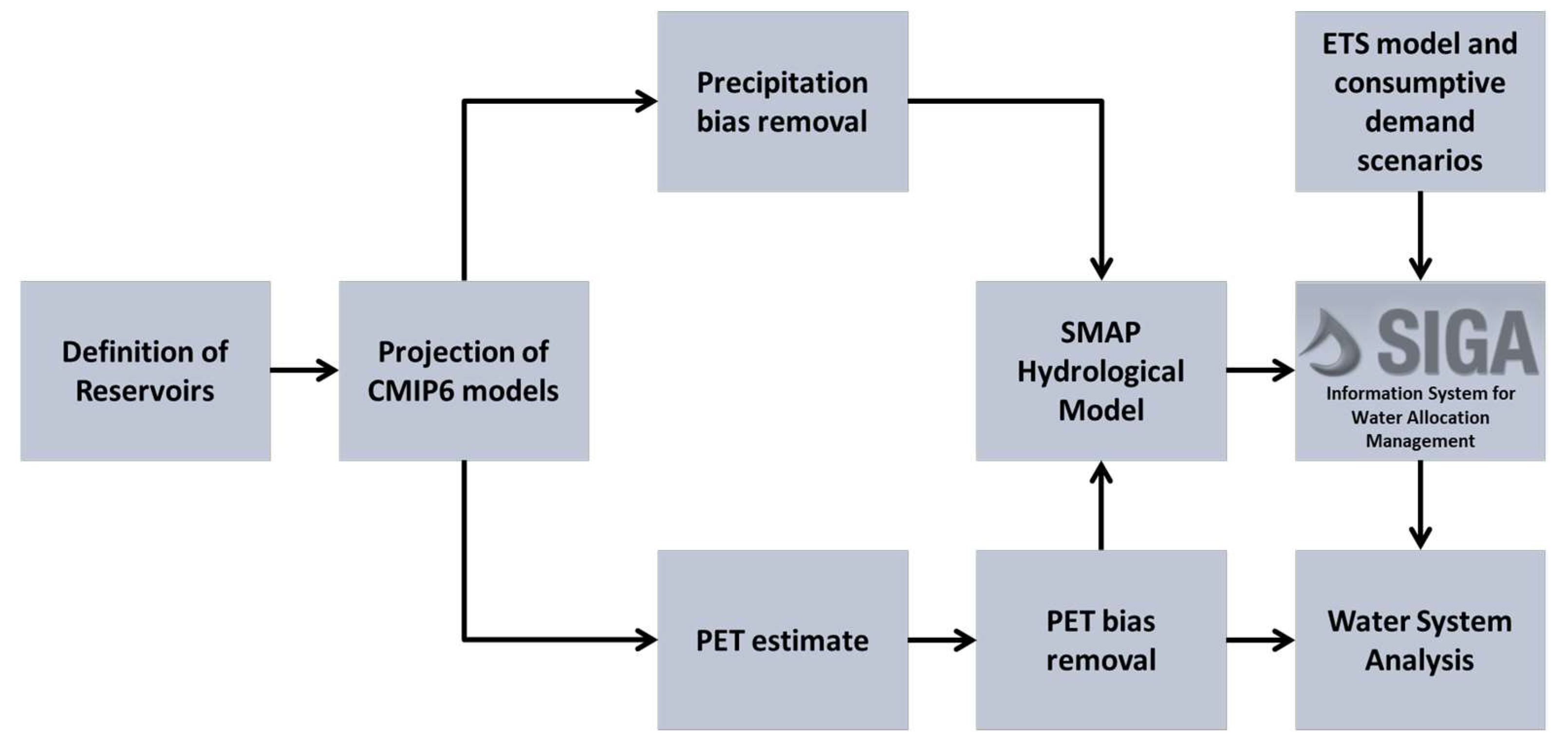
Figure 2.
Monthly SMAP, schematic diagram of operation. Source: [17].
Figure 2.
Monthly SMAP, schematic diagram of operation. Source: [17].
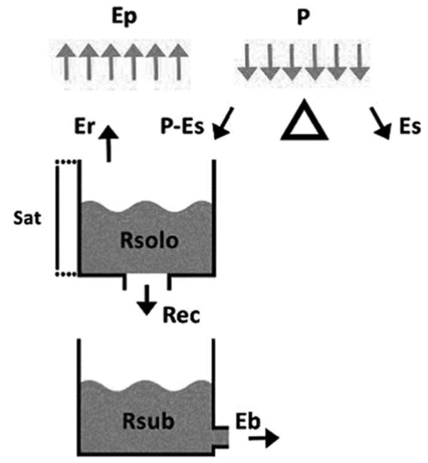
Figure 3.
Illustration of the network used for water system operation in SIGA®.
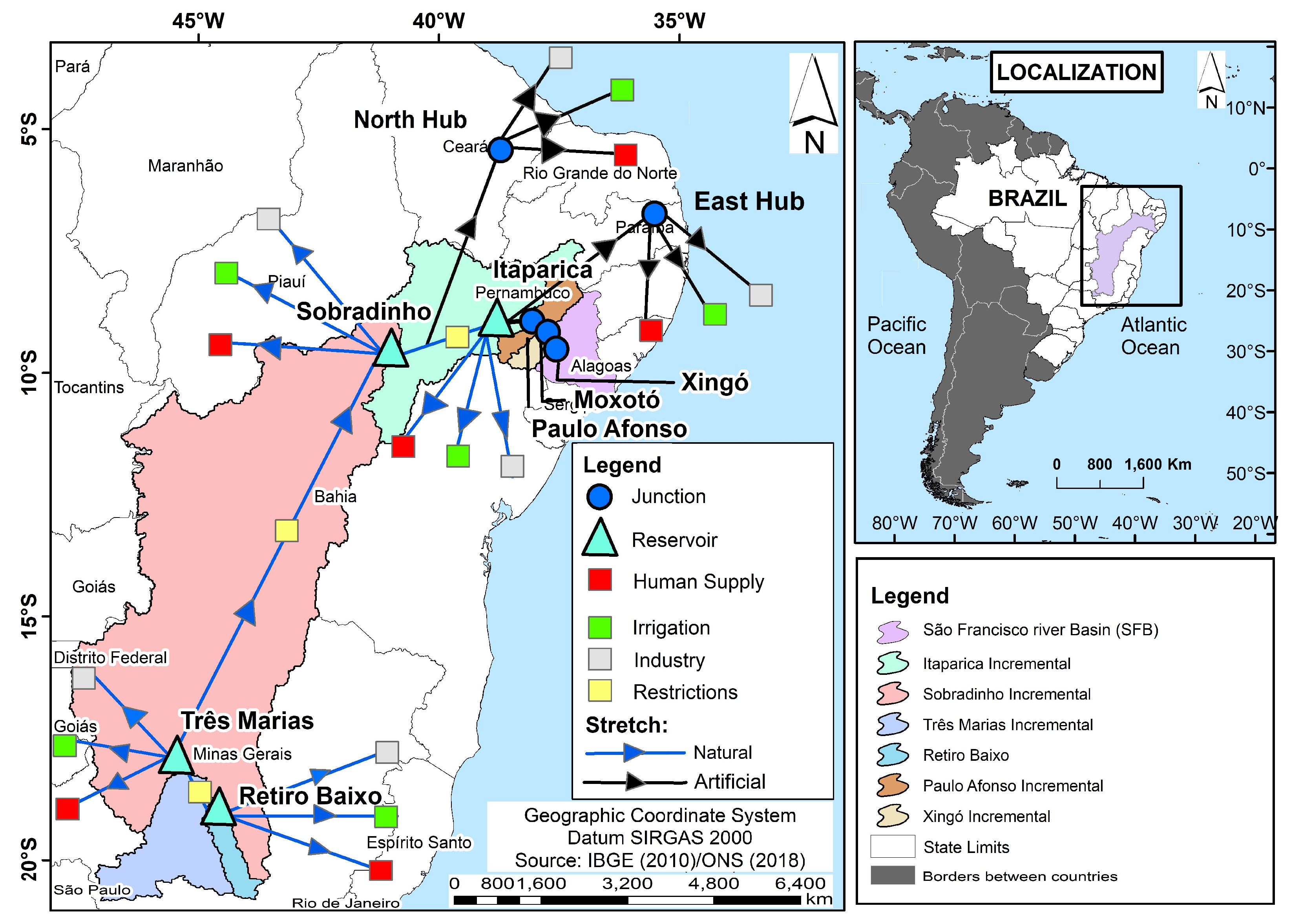
Figure 4.
Simulated Flow – Calibration (1996 to 2005) and Validation (2006 to 2017) results.
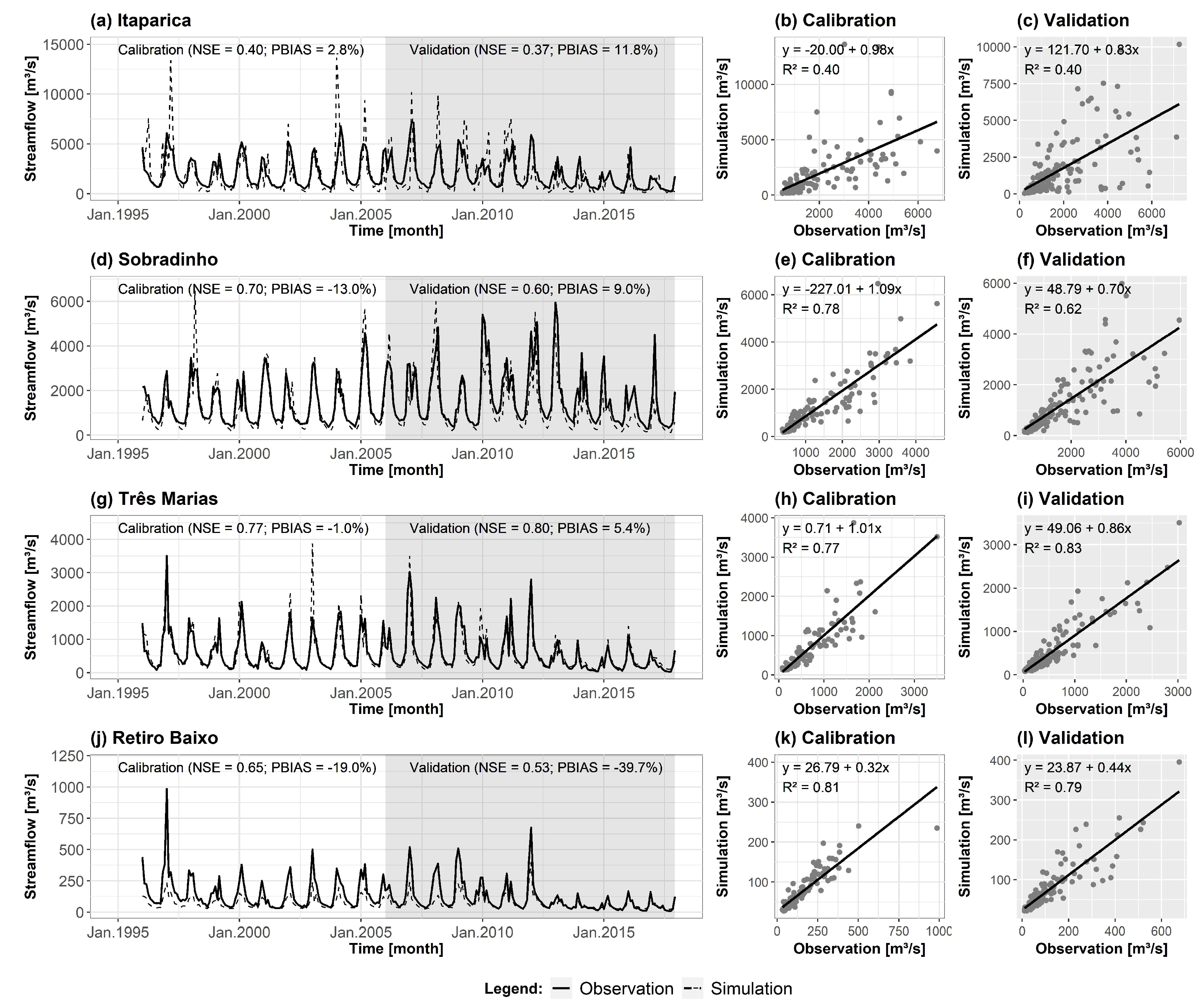
Figure 5.
Seasonality of the CMIP6 models compared to the observed precipitation.
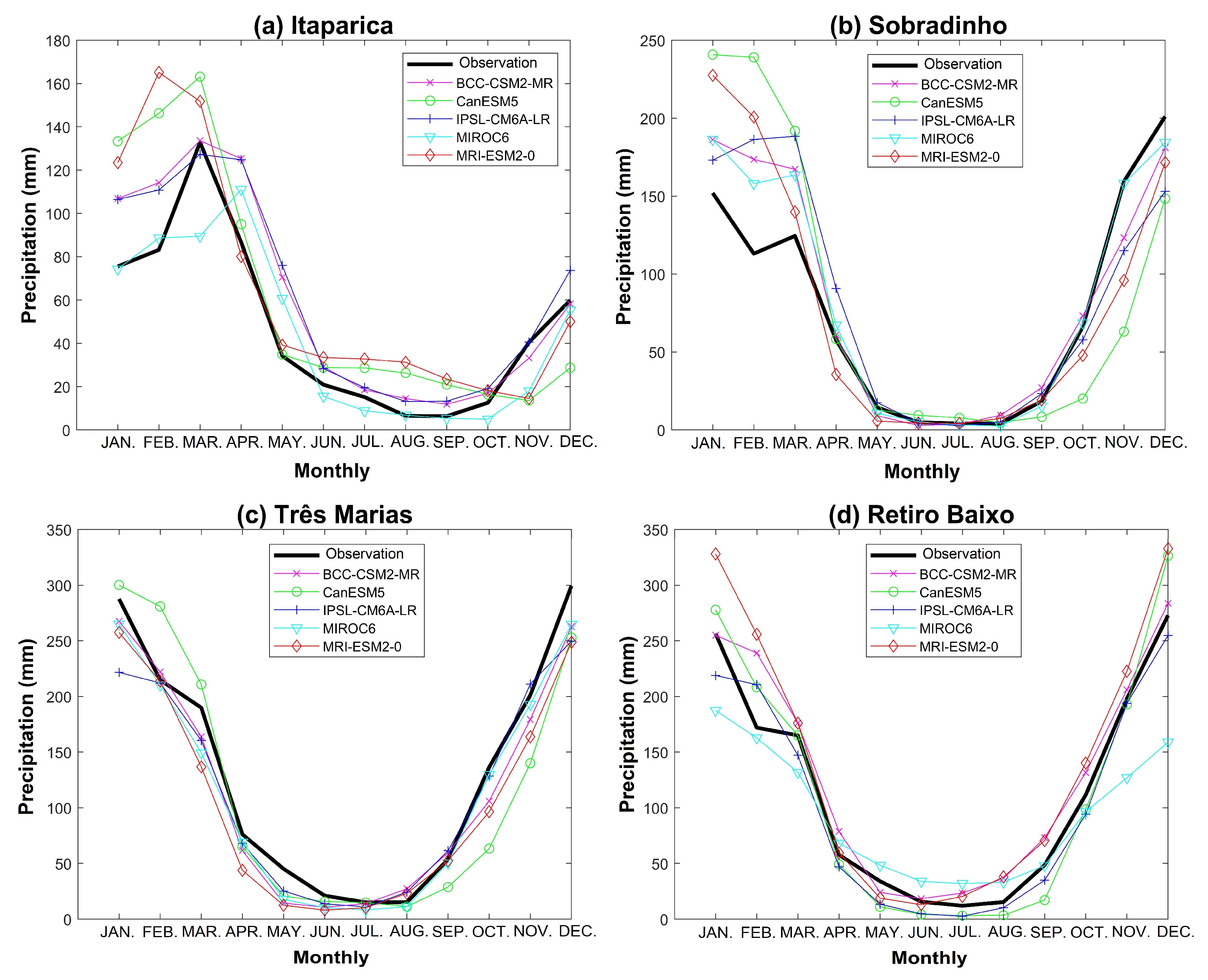
Figure 6.
Taylor Diagram of the precipitation seasonality of the CMIP6 models in relation to observed data.
Figure 6.
Taylor Diagram of the precipitation seasonality of the CMIP6 models in relation to observed data.
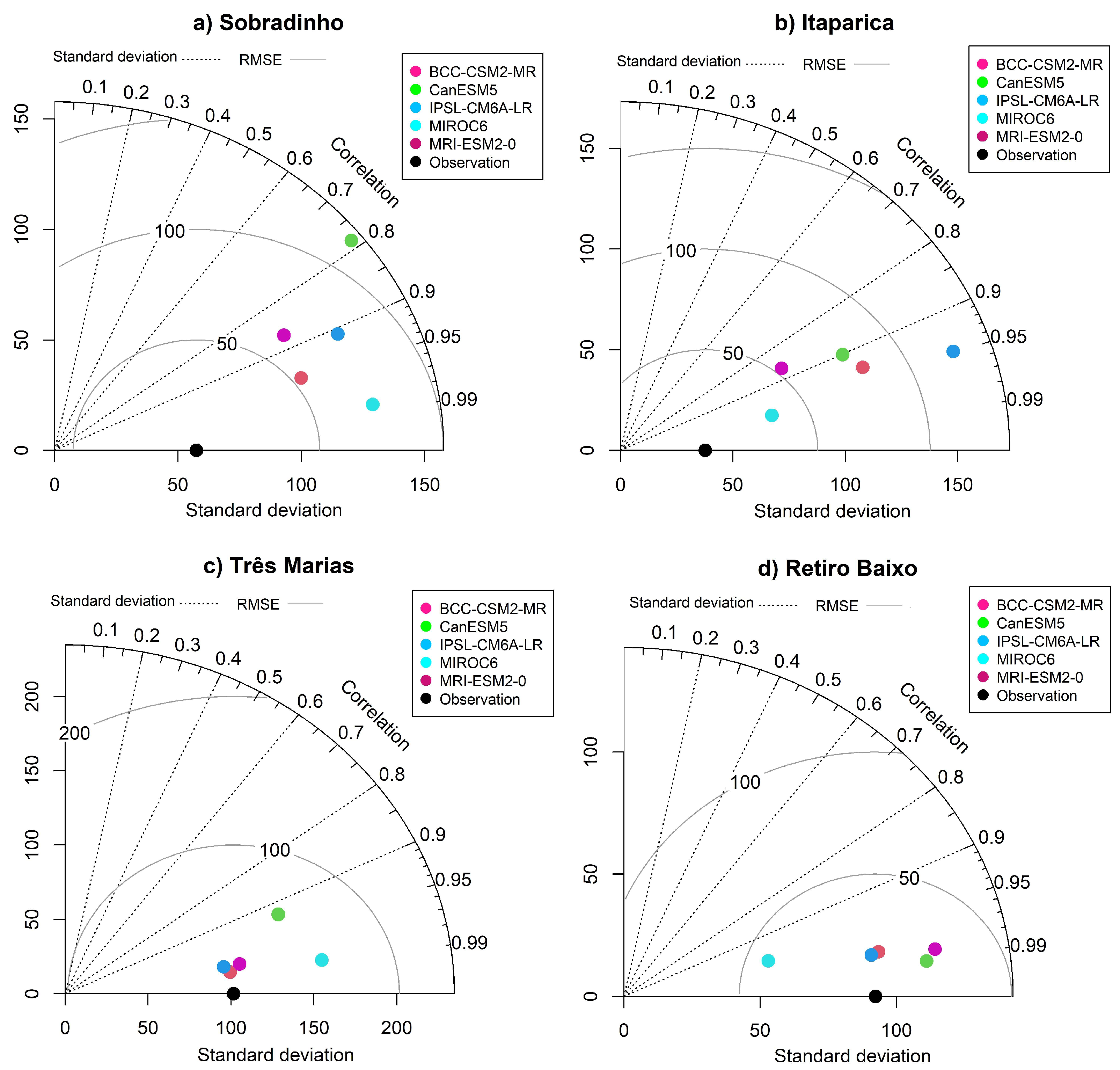
Figure 7.
Percentual Anomalies of the PET, Precipitation and Mean Annual Streamflow from CMIP6 models.
Figure 7.
Percentual Anomalies of the PET, Precipitation and Mean Annual Streamflow from CMIP6 models.
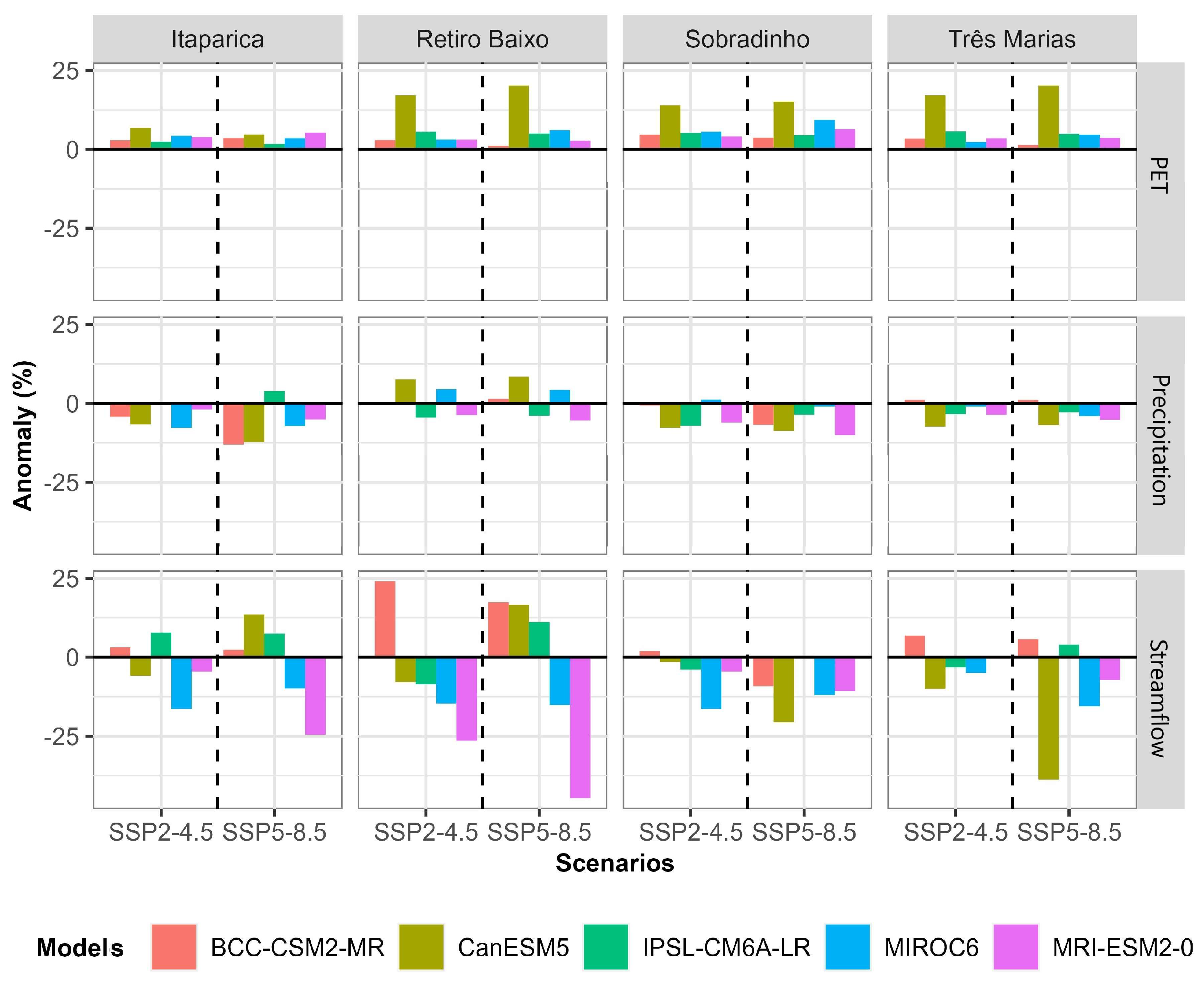
Figure 8.
Historical consumptive demands and future scenarios (D1, D2, D3 e D4).
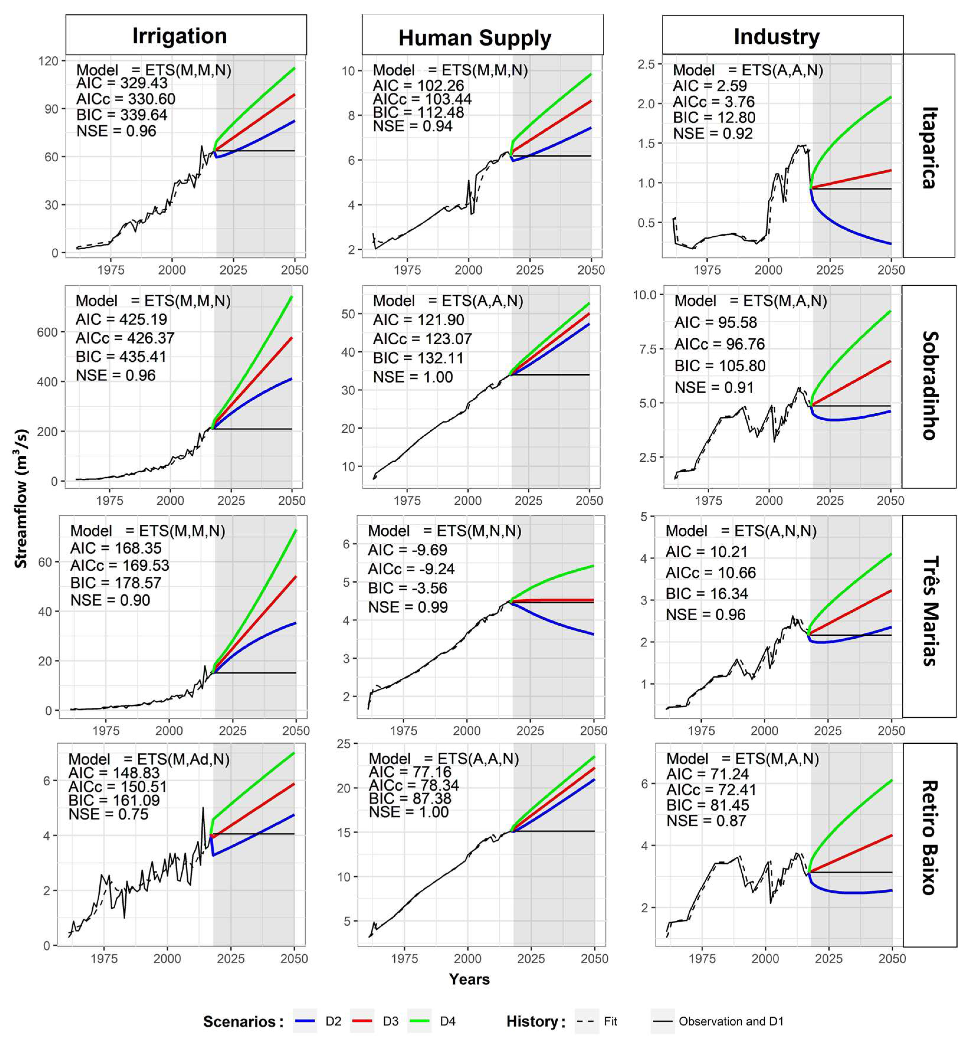
Figure 9.
Reliability Index of CMIP6 models for historical period (1971 to 2000), climate change scenarios (SSP2-4.5 and SSP5-8.5) and consumptive demands projection scenarios (D1, D2, D3 and D4) for SFRB reservoirs. The bars are the averages of the set of models.
Figure 9.
Reliability Index of CMIP6 models for historical period (1971 to 2000), climate change scenarios (SSP2-4.5 and SSP5-8.5) and consumptive demands projection scenarios (D1, D2, D3 and D4) for SFRB reservoirs. The bars are the averages of the set of models.
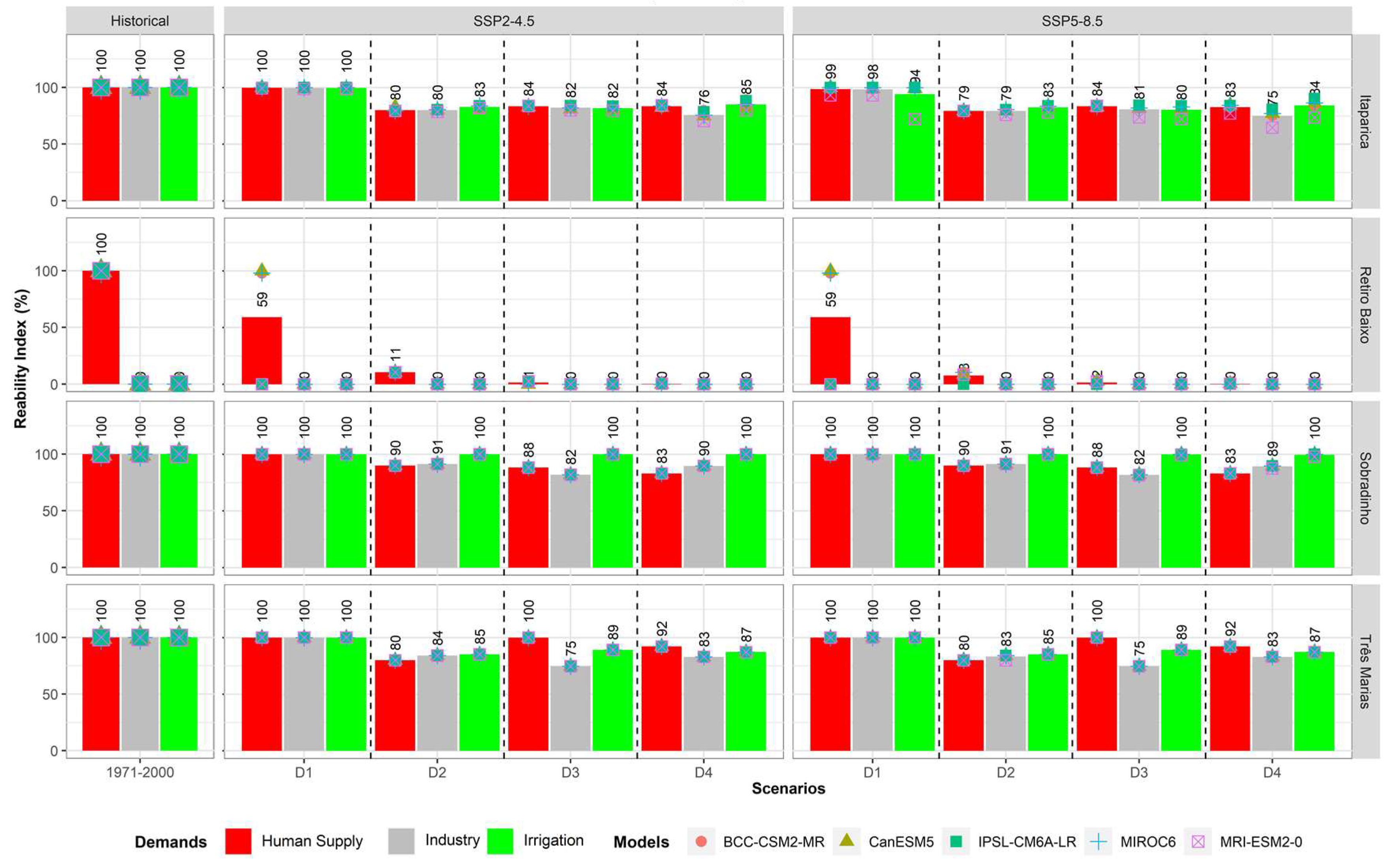
Figure 10.
Resilience Index of CMIP6 models for historical period (1971 to 2000), climate change scenarios (SSP2-4.5 and SSP5-8.5) and consumptive demands projection scenarios (D1, D2, D3 and D4) for SFRB reservoirs. The bars are the averages of the set of models.
Figure 10.
Resilience Index of CMIP6 models for historical period (1971 to 2000), climate change scenarios (SSP2-4.5 and SSP5-8.5) and consumptive demands projection scenarios (D1, D2, D3 and D4) for SFRB reservoirs. The bars are the averages of the set of models.
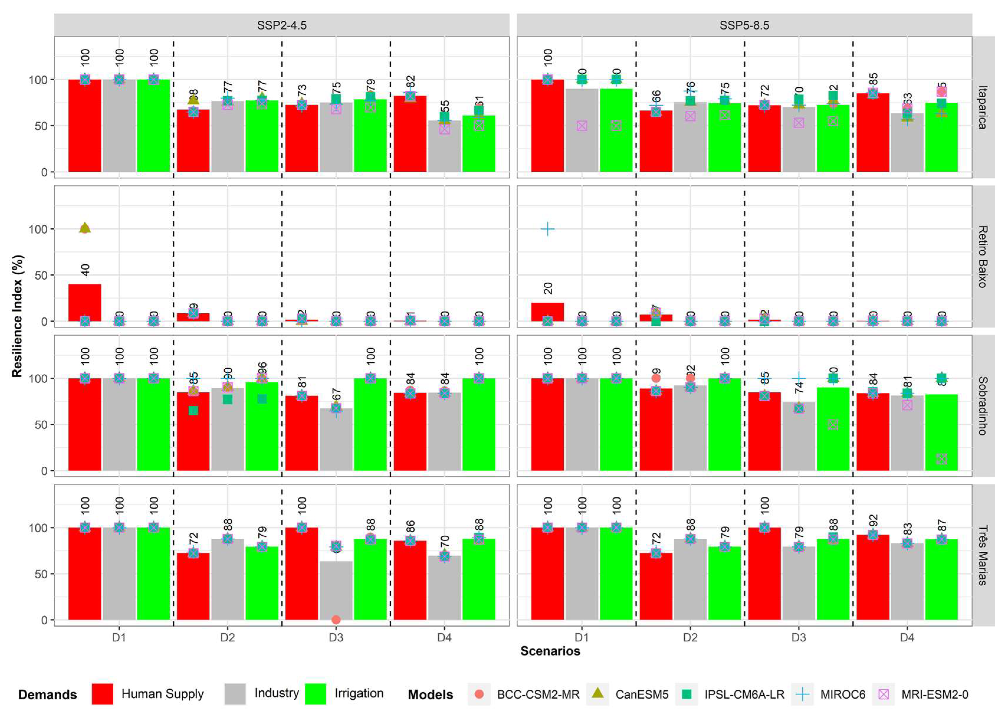
Figure 11.
Vulnerability Index of CMIP6 models for historical period (1971 to 2000), climate change scenarios (SSP2-4.5 and SSP5-8.5) and consumptive demands projection scenarios (D1, D2, D3 and D4) for SFRB reservoirs. The bars are the averages of the set of models.
Figure 11.
Vulnerability Index of CMIP6 models for historical period (1971 to 2000), climate change scenarios (SSP2-4.5 and SSP5-8.5) and consumptive demands projection scenarios (D1, D2, D3 and D4) for SFRB reservoirs. The bars are the averages of the set of models.
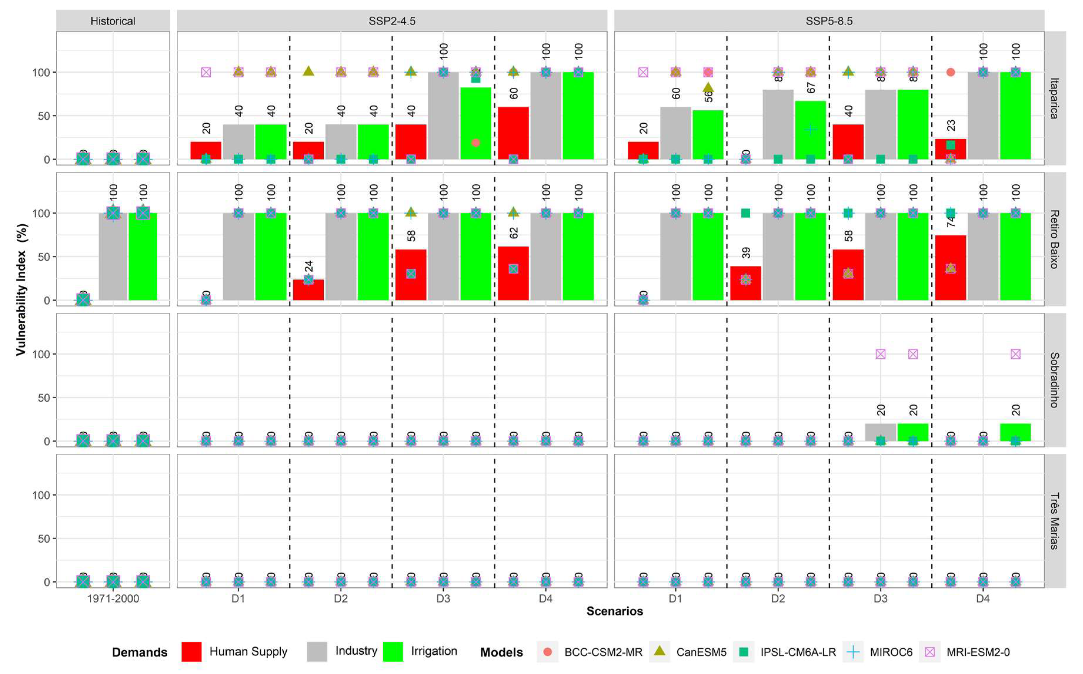
Figure 12.
Sustainability Index of CMIP6 models for historical period (1971 to 2000), climate change scenarios (SSP2-4.5 and SSP5-8.5) and consumptive demands projection scenarios (D1, D2, D3 and D4) for SFRB reservoirs. The bars are the averages of the set of models.
Figure 12.
Sustainability Index of CMIP6 models for historical period (1971 to 2000), climate change scenarios (SSP2-4.5 and SSP5-8.5) and consumptive demands projection scenarios (D1, D2, D3 and D4) for SFRB reservoirs. The bars are the averages of the set of models.
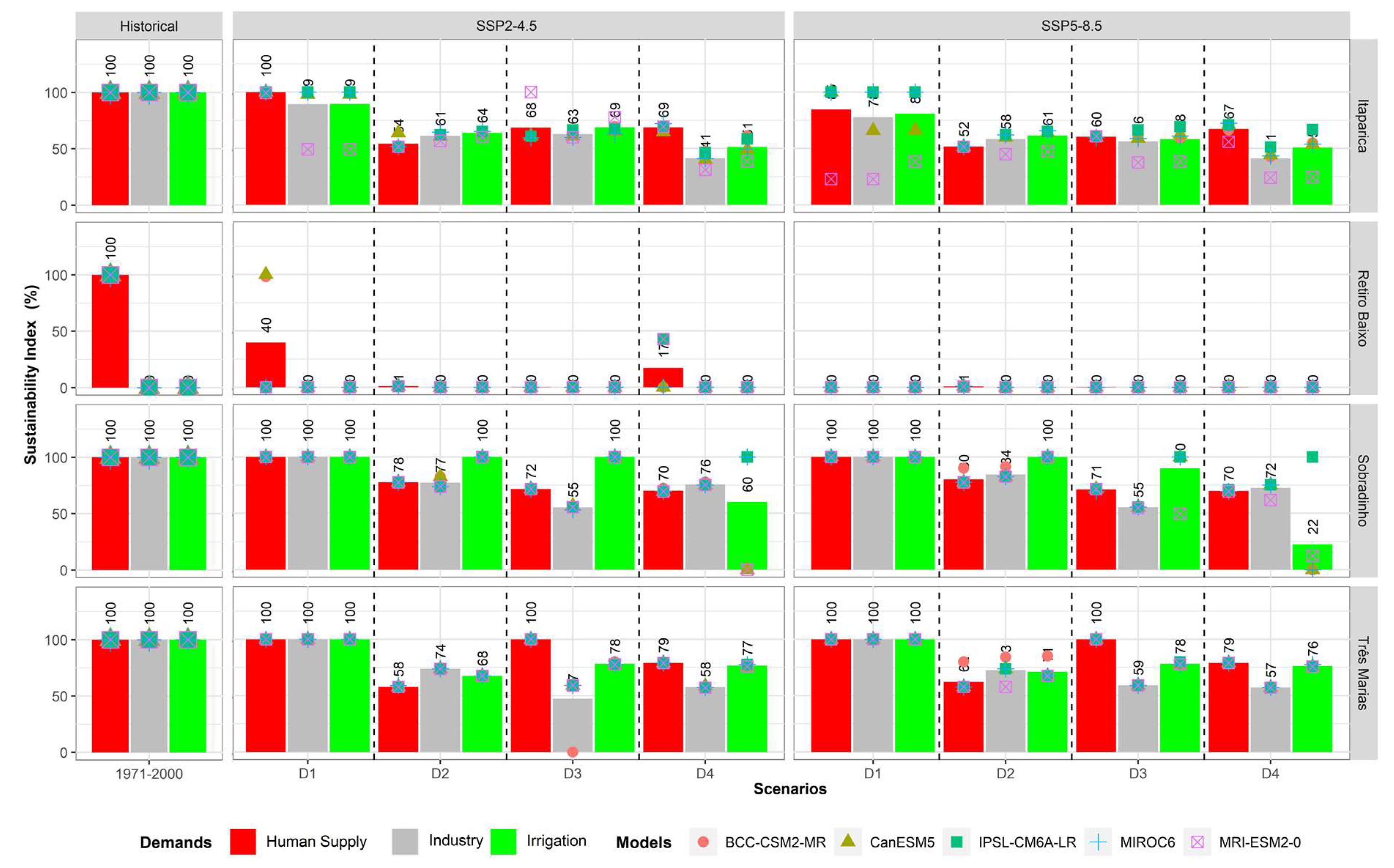

Table 1.
CMIP6 models with their respective responsible institutions, countries and quotes.
| Modelos | Instituição ou Organização (Países) | Citações |
|---|---|---|
| CanESM5 | Canadian Earth System Model 5th generation (Canadá) | [12] |
| IPSL-CMSA-MR | Institut Pierre-Simon Laplace (França) | [13] |
| MIROC6 | Atmosphere and Ocean Research Institute, National Institute for Environmental Studies, and Japan Agency for Marine-Earth Science and Technology (Japão) | [14] |
| BCC-CSM2-MR | Beijing Climate Center climate system model version 2 (China) | [15] |
| MRI-ESM2-0 | Meteorological Research Institute Earth System Model version 2 (Japão) | [16] |
Table 2.
SMAP parameters and initializations after calibration. Also, basin period and calibration period.
Table 2.
SMAP parameters and initializations after calibration. Also, basin period and calibration period.
| Basin | Área (km²) | Calibration Period | TUin | EBin | SAT | Pes | CREC | K |
| Retiro Baixo | 12,187 | 01/1996 a 12/2006 | 68.66 | 54.74 | 3,240.12 | 8.34 | 1.89 | 0.09 |
| Três Marias | 50,732 | - | 86.36 | 212.83 | 1,769.15 | 8.05 | 2.6 | 0.02 |
| Sobradinho | 467,000 | - | 60.7 | 751.65 | 1,500.14 | 5.75 | 4.10 | 0.01 |
| Itaparica | 93,188 | - | 97 | 322 | 5,000 | 5.6 | 0.69 | 13.25 |
Table 3.
Operating restrictions downstream of the reservoirs.
| Reservoir | Minimum Streamflow (m3/s) | Maximum Streamflow (m3/s) |
|---|---|---|
| Três Marias | 100 | 2500 |
| Sobradinho | 700 | 8000 |
| Itaparica | 700 | 8000 |
Table 4.
Priority ranking for reservoir system simulation.
| Demand | Priority |
|---|---|
| Human Supply (HS) | 1 |
| Transposition (TRA) | 2 |
| Irrigation (IRR) | 3 |
| Industry (IND) | 4 |
Table 5.
Mean annual growth rate of consumptive demands.
| Reservoir | Demands | Mean annual growth rate (%) | |||
| Historical (1961-2017) | D2 | D3 | D4 | ||
| Itaparica | Irrigation | 6.80 | 0.81 | 1.35 | 1.73 |
| Human Supply | 1.88 | 0.54 | 0.95 | 1.25 | |
| Industry | 2.87 | 3.73 | 0.66 | 2.46 | |
| Sobradinho | Irrigation | 7.42 | 1.41 | 2.93 | 3.80 |
| Human Supply | 3,03 | 0.97 | 1.18 | 1.36 | |
| Industry | 2,53 | 0.70 | 1.07 | 1.99 | |
| Três Marias | Irrigation | 10,99 | 1.80 | 3.70 | 4.62 |
| Human Supply | 1,84 | 1.02 | 0.02 | 0.77 | |
| Industry | 3,53 | 0.08 | 1.19 | 1.93 | |
| Retiro Baixo | Irrigation | 9,29 | 1.10 | 1.27 | 1.37 |
| Human Supply | 2,99 | 0.97 | 1.16 | 1.34 | |
| Industry | 2,15 | 1.53 | 0.99 | 2.06 | |
Disclaimer/Publisher’s Note: The statements, opinions and data contained in all publications are solely those of the individual author(s) and contributor(s) and not of MDPI and/or the editor(s). MDPI and/or the editor(s) disclaim responsibility for any injury to people or property resulting from any ideas, methods, instructions or products referred to in the content. |
© 2023 by the authors. Licensee MDPI, Basel, Switzerland. This article is an open access article distributed under the terms and conditions of the Creative Commons Attribution (CC BY) license (http://creativecommons.org/licenses/by/4.0/).
Copyright: This open access article is published under a Creative Commons CC BY 4.0 license, which permit the free download, distribution, and reuse, provided that the author and preprint are cited in any reuse.


