Preprint

Article

Emissions and CO2 Concentration – an Evidence Based Approach

Altmetrics

Downloads

313

Views

294

Comments

A peer-reviewed article of this preprint also exists.

This version is not peer-reviewed

Submitted:

19 February 2023

Posted:

23 February 2023

You are already at the latest version

Alerts

Abstract

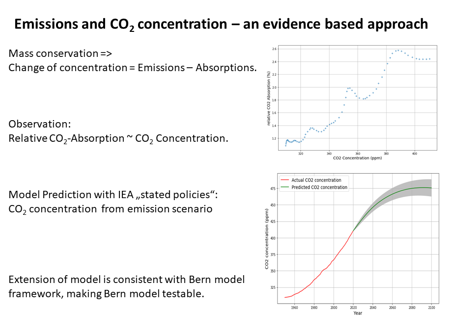
The relation between CO2 emissions and atmospheric CO2 concentration has traditionally been treated with more or less complex models with several boxes. Our approach is motivated by the question of how much CO2 must necessarily be absorbed by sinks. Observations lead to the model assumption, that carbon sinks like oceans or biosphere are linearly dependent on CO2 concentration on a decadal scale. In particular this implies the falsifiable hypothesis that oceanic and biological CO2 buffers have not significantly changed in the past 50 years and are not saturated in the forseeable future. The simple model with 2 parameters explains very well the CO2 emission and historical CO2 concentration data. The model gives estimates of the natural emissions, the pre-industrial CO2 equilibrium concentration levels, the half-life time of an emission pulse, and the future CO2 concentration level from a given emission scenario. This is validated by an ex-post forecast of the last 20 years. The important result is that with the stated polices scenario of the IEA future CO2 concentrations will not rise above 475 ppm. The model is compared with the Carbon modul of the Bern model, mapping their complex IRFs to a single time variant parameter.

Keywords:

Subject: Environmental and Earth Sciences - Atmospheric Science and Meteorology

1. Introduction—A New Way of Looking at the Problem

Climate science is usually concerned about the question “How much CO₂ remains in the atmosphere?”, given the anthropogenic emissions, and the limited capability of oceans and biosphere to absorb the surplus CO₂ concentration [1,2,3,4] This has lead to conclusions of the kind that a certain increasing part of anthropogenic emissions will remain in the atmosphere forever.

We change the focus of attention by posing the logically equivalent question “How much CO₂ does not remain in the atmosphere?”. Why is this so different? The amount of CO₂ that does not remain in the atmosphere can be calculated from direct measurements. We do not have to discuss each absorption mechanism from the atmosphere into oceans or plants, but from the known concentration changes and the known emissions we have a good estimate of yearly actual absorptions. These are related to the CO₂ concentration, motivating the guiding hypothesis for a linear model of absorption. It turns out that we do not need to know the actual coefficients of the different absorption mechanisms, it is sufficient to assume a linear dependence on the current CO₂ concentration.

Additionaly by changing the focus of attention from “how much remains in the atmosphere” to “how much is absorbed annually”, the formally equivalent estimation equations become much better conditioned. Both known previous investigations based on a linear absorption model [5,6] had computational stability problems, noticable in the large error bars of the resulting equlibrium concentration. Although the publications omit the computation of error bars, from their data and equations they can be reproduced. A third paper with a linear absorption model [7] uses apparently similar equations, but separates the estimation of the oceanic and biosphere absorption constants from the contribution of anthropogenic emissions, which leads to the strange phenomenon that their main equation has no more free parameters to react on emission changes explicitely. We will discuss their approach in the appendix.

2. The Absorption Model

2.1. Mass Conservation

From the Global Carbon Project [8] we get the emission and concentration data. A global mass balance representation of the yearly atmospheric CO₂ flow is created, with

C_i as the CO₂ concentration of the atmosphere at the end of year i,
E_i as the global emissions of human origin during year i,
L_i as the global land use net emissions during year i,
N_i the global natural net emissions during year i,
S_i other special causes of emissions such as El Nino, vulcanos, etc.
A_i as the global net absorption of CO₂ during year i into the oceans and biosphere ( $0 < = i < n$ )

$\begin{matrix} C_{i} & = & C_{i - 1} + E_{i} + L_{i} + S_{i} + N_{i} - A_{i} \end{matrix}$

(1)

Without explicit external information, $S_{i}$ cannot be discriminated from $L_{i}$ or $N_{i}$ . Therefore we set $S_{i}$ to 0, and include all inferred special causes in the unknown $N_{i}$ in this investigation. With $S_{i} = 0,$ the equation becomes

$\begin{matrix} E_{i} + L_{i} - (C_{i} - C_{i - 1}) & = & A_{i} - N_{i} \end{matrix}$

(2)

This is not a model, but the formulation of the necessary mass conservation as seen from the atmosphere—like a bank account with cumulative yearly deposits and withdrawals, not directly dealing with the daily ups and downs nor with the exact nature of the earning and spending processes. As a matter of fact, equation (2) must be fulfilled at all time scales.

For consistency all quantities have to be converted to the same unit (1 ppm = 2.124 GtC, 1 GtC = 3.664 Gt CO₂ [8]). Here all calculations here are done with the unit “ppm”. All CO₂ related data, emissions, land use change, and CO₂ concentration growth are from the Global Carbon Budget 2021, covering the years 1850-2020. We have to be aware that the land use change data are subject to considerable uncertainty, with an error range of

\pm 0.4

ppm.

Consistency reasons will justify to assume an estimate for land use change emission that is 0.2 ppm lower than the published mean value. This is well within the error range and therefore justifiable.

Figure 1 shows that the total emissions (

E_{i}

L_{i}

, blue) exceed the yearly CO₂ concentration growth (

C_{i} - C_{i - 1}

, green) increasingly, indicating that we have an increasing effective absorption (

A_{i} - N_{i}

, red ) with growing CO₂ concentration.

One immediate result of displaying these raw data is that before 1900 the anthropogenic emissions were considerable smaller than other variations such as land use change. There are roughly 4 historical phases:

The phase before 1900, where explicit emissions are smaller than implicit ones by land use change, however there is a small but increasing CO₂ concentration growth,
the phase between 1900 and 1950 with growing emissions but approximately constant CO₂ concentration growth and slightly increasing land use change,
the phase from 1950 to 2010 with growing emissions and growing concentration growth.
Recent publications indicate that emissions have remained approximately constant since 2010 [9] and are expected to remain approximately constant for the forseeable future [10] (Figure 2, Stated Policies Scenario). The challenge is to estimate reasonable projections of CO₂ concentration based on these emission assumptions.

2.2. Exploratory Analysis

As a first exploratory analysis of these data, the scatter plot in Figure 2 relates the effective CO₂ absorption to the CO₂ concentration.

Qualitatively we see a long term linear dependence of the effective absorption on the atmospheric CO₂ concentration with significant short term deviations, where the effective zero-absorption line is crossed at appr. 280 ppm. This is considered to be the pre-industrial equilibrium CO₂ concentration where natural yearly emissions are balanced by the yearly absorptions. The average yearly absorption is appr. 2.5% (

\frac{1}{40}

)of the CO₂ concentration exceeding 280 ppm.

While the correlation coefficient of 0.97 is very high, there are clear non-random deviations from an ideal linear behaviour. With the large uncertainty of the land use change, and contingent effects such as vulcano eruptions, influences like ENSO, etc., it is not surprising that there are systematic deviations from a perfect line [6].

Regarding predictions of future CO₂ concentration, the key question is, whether the deviations are averaging out or whether there is a systematic saturation trend, limiting the absorption of CO₂. Some climate researchers claim that the absorption will decline [11], but there are other papers providing evidence of increasing absorption [12].

We can see from these data, that a reliable estimate of the historical equilibrium concentration requires the whole data range. An estimation based on all data above 310 ppm (year 1950) would result in a smaller equilibrium value of 245 ppm.

Starting from the mass conservation equation above, on the basis of the preceding considerations, we state two hypotheses, from which the actual model is derived:

2.3. Hypothesis 1: The Absorption $A_{i}$ Is Proportional to Previous CO₂ Concentration

Formally this is

\begin{matrix} A_{i} & = & a \cdot C_{i - 1} \end{matrix}

(3)

The physical justification for this assumption is the fact that the partial pressure of CO₂, which is relevant for absorption processes, increases proportional to concentration. It is also known that C3 plants, representing the majority of all plants, have a linear absorption property. The absorption property of C4 plants is nearly flat, but also linear in the range of 280-560 ppm, resulting in a linear behaviour when averaging over all plants. Ari Halperin analysed the different processes of gas transport into the ocean, with the conclusion that all relevant processes can be linearized [5], equation 16.

Assuming that there are different absorption constants for oceanic (

a_{O c e a n}

) and biospheric absorption (

a_{B i o s p h e r e}

), under the linearity assumtion they can be added to a single constant a:

\begin{matrix} a & = & a_{O c e a n} + a_{B i o s p h e r e} \end{matrix}

(4)

Both ocean as well as biospheric processes may consist of multiple sub-processes. E.g. the photosynthesis of C3 plants has a much larger proportionality constant to that of C4 plants in the relevant CO2 concentration range of 280..560 ppm. As long as linearity holds, the net absorption constant is reflected by the sum of all elementary absorption constants.

This is a radical simplification of the box-diffusion model [13] referred to in the article “ Predicting Future Atmospheric Carbon Dioxide Levels“ [1]. Instead of assuming separate boxes for the mixed layer and for the biosphere, we assume a one-dimensional diffusion process between atmosphere and ocean resp. biosphere with a single diffusion constant, making no explicit assumptions about the properties of the mixed layer nor the mechanism of the absorption in the biosphere. As stated above, this is justified when all relevant absorption processes are approximately linear w.r.t. CO₂ concentration. The advantage of this model is that we do not have to make any speculative assumptions about potentially many model parameters, some of which are quite arbitrary (e.g. thickness of mixed layer), but restrict the whole model to a single absorption parameter, which can be estimated from measurable data.

The authors of the Bern model claim, that the “net primary production of the land biosphere and the surface ocean carbon uptake depend on atmospheric CO₂ and surface temperature in a nonlinear way” [4] by assuming a superposition of 4 linear processes. This statement contradicts our assumption of a single linear process. We will show in the appendix that the IRF’s of the Bern model [4], Equation (21)), can be mapped into the form of our model with a time varying absorption parameter a. Statistical tests will tell if there is a need to actually introduce this time dependence or whether it is more appropriate to assume constant relative absorption over time. Any deviations from the validity of a linear model will show up in the residual error. This gives our model a method of intrinsic validation, and the model can be extended when required.

2.3.1. Temperature Dependence of the Absorption Parameter

We have to consider the possibility that the absorption parameter a depends on temperature. Investigations of ice-core data clearly indicate a temperature dependency of CO₂ concentration. The open question is whether there is a measurable dependency during the time scale and the temperature scale of our investigation. We will hypothetically test the temperature dependence of relative absorption a with a linear dependency on sea surface temperature anomalies T, with the HadSST2 temperature

T_{i}

[14]. Linear dependence on Temperature anomaly is assumed like in the Bern model [4]:

a_{i} = a_{0} + a_{1} \cdot T_{i}

(5)

2.3.2. CO₂ Concentration as a Hypothetical Proxy for Temperature

When we make predictions with hypothetical future CO₂ emissions, we don’t know future temperatures. Without diving into the problematic discussion about the degree, how strong the influence of CO₂ concentration is on temperature, we assume the “worst case” of full predictability of temperature effects by CO₂ concentration (Figure 3).

Without making any assumptions about C_i−1→T_i causality, the estimated functional dependence of the temperature proxy from the regression with CO₂ concentration is

T_{i}^{p r o x y} = - 16.0 + 2.77 \cdot ln (C_{i - 1})

(6)

We are aware that this is a very incomplete model, because it ignores the obvious significant, trend reversing deviations between 1900 and 1975, and it also ignores the dominant contribution of cloud albedo reduction to global warming [15], whereby 80% of recent warming is caused by albedo reduction and only 20% by increase of CO₂ concentration. The proxy is still suitable as a tool for estimating an upper bound of temperature dependence on CO₂ concentration. Based on actually measured data, it avoids speculations and discussions about hypothetical feedback factors of CO₂ sensitivity.

2.3.3. Corollary: Carbon Sinks Are Not Expected to Be Saturated in the Near Future

This is related to and is a consequence of the linearity assumption. Much of the debate about carbon sinks is concerned with numerous details about possible saturation of various “boxes” in the models. There are strong reasons to consider the atmosphere and the mixed layer, i.e. the top 75 m of the ocean as a single “box”, which exchanges gases with the deep ocean and the biosphere [5]. Due to the fact that the deep ocean contains more than 50 times the CO₂ of the atmosphere, or 4000 times the yearly global emissions, this means, that the whole atmospheric content is just about 2% of the ocean content. Therefore we do not expect this huge “box” to be saturated any time soon.

Having said that, we do not rely on our own assumptions, but there are 4 indications supporting the assumption that the uptaking reservoirs are not saturated:

We can test the past 70 years for linearity. If there was any sign of saturation, this would have shown up as a deviation from the linearity assumption. We will see that in the residual deviations from the model: if the relative absorption decreases with time, the real CO₂ content at the end would be larger than estimated by the linear model.
The global carbon budget [8] clearly shows an increasing trend in both the ocean sink as well as the (biosphere) land sink.
A recent article revised the estimates of the ocean-atmosphere CO₂ flux [12], making it consistent with the increasing ocean sink found in the global carbon budget.
We can make a rough estimation of the expected ocean uptake. The ocean has a total carbon inventory of 38000 GtC ≈140000 Gt CO₂. If we assume the realistic scenario of constant future emissions at today’s level (37 Gt CO₂ per year) and we assume that they are all absorbed by the ocean, by 2100 that would be appr. 3000 Gt CO₂, just about 2% of the current inventory.

Whatever the subjective opinion is regarding the future absorption, the measured data provide us with the current trend and its potential changes in the near future.

2.4. Hypothesis 2: Natural Emissions and Absorptions Are Balanced

This implies that without anthropogenic emissions

C_{i}

C_{i - 1}

C_{0}

, resulting in a constant equilibrium concentration

C_{0}

. Equations (1)–(3) imply that global natural emissions are constant:

\begin{matrix} N_{i} & = & a \cdot C_{0} \end{matrix}

(7)

This relation makes a falsifiable statement about the magnitude of those natural emissions, which are not compensated by absorptions within the time unit of measurement, which is a year in this investigation. The statement of assumed constant equilibrium concentration requires further clarification. We know e.g. from ice-core investigations that historical CO₂ concentration is not constant, and most likely depends on temperature. A linear dependence on temperature can be mapped onto a linear dependence of relative absorption a on temperature, which is covered by equation (5).

As we know, there are causes for systematic changes in the natural emissions, e.g. vulcano eruptions, ocean cycles, or changes of land use. We will see from the residual deviations of the measured data, how significant these influences are, and if the model needs to be adapted. For the time being, we initially assume no changes of natural emissions within the investigated time range 1850-2020. As with the previous assumption, the residual error of the model will lead to possible further fine-tuning of the model. Three possible deviations are possible:

a systematic “trend” in the natural emissions. This would either increase or decrease the estimated absorption factor and the equilibrium concentration, resp. the constant model of natural emissions,
short term zero centered variations within a year. These variations do not show up in our model due to the one year sampling interval,
long term variations of more than a year are not averaged out. They a are visible in the residual error of the predicted CO₂ content.

2.5. The Modelling Equations

From equation (2), (3), and (7) we get the final model equation for an assumed constant absorption parameter a:

E_{i} + L_{i} - (C_{i} - C_{i - 1}) = a \cdot C_{i - 1} - a \cdot C_{0}

(8)

Equation (8) emphasises the fact that the effective absorption depends on the difference betwees the actual and the equilibrium CO₂ concentration

C_{0}

, implicitely including the natural carbon cycle, described by the equlibrium concentration

C_{0}

. Initially we estimate

a \cdot C_{0}

as the constant natural emissions simultaneously with a in this regression equation, for estimating temperature dependent models we assume a fixed known value for the equilibrium CO₂ concentration

C_{0}

and estimate the absorption function a.

Starting with the available data, from emissions

E_{i}

, land use change

L_{i}

, CO₂ growth, the absorptions are modelled according to equation (8) for the time interval 1850-2014,

For

L_{i}

, the emission change per year due to land use, the uncertainty is considerable [8]. Therefore we have a certain amount of freedom to adapt its value in order to satisfy other given constraints.

The absorption constant a and the natural equilibrium concentration

C_{0}

in a given time interval are obtained through estimation with the least-squares method, where the dependent variable is the left hand side of equation (8), the independent variable is

C_{i - 1}

, by means of the Python module OLS (statsmodel-OLS-0.13.5). The result table of the Python linear regression model displays for each regression variable its estimated value (Coef.), its estimated standard error, the t-statistics for the variable being different from 0, the probability for the variable to be 0 (strictly speaking the error probability when accepting the hypothesis that the variable is different from 0), and in the last 2 colums the error bounds, i.e. the 95% interval of the variable’s value:

	Coef.	Std.Err.	t	$P > \| t \|$	[0.025	0.975]
$- a \cdot C_{0}$	-6.8952	0.2640	-26.1142	0.0000	-7.4166	-6.3738
a	0.0247	0.0008	29.3485	0.0000	0.0230	0.0264

This results in

C_{0} = 279

ppm, with error bounds [277, 282] ppm, and a half life time of an emission pulse

t_{1 / 2} = \frac{ln (2)}{a} = 28

years, with error bounds [26,30] years.

C_{0}

is very close to and its error bounds contain the widely accepted pre-industrial equilibrium CO₂ concentration of 280 ppm. As it can be seen from model equation (8), we can substitute global variations of

L_{i}

and

C_{0} :

Δ C_{0} = - \frac{1}{a} Δ L

(9)

When using the center value of the land use change error band, i.e. on average 0.55 ppm , the calculated

C_{0}

would have been

271 \pm 2

ppm, which we consider to be too small to be compatible with the accepted value of 280 ppm. Therefore in the face of the large uncertainty of land use change estimates we prefer to assume slightly lower average land use change caused emissions (average 0.35 ppm) over an inconsistent equilibrium concentration. This substitution, however, only changes the equilibrium concentration.

Modelling the raw, noisy differential absorption data with this – simplest possible – model shows a fairly good approximation over the whole time span. The residue

R_{i} = E_{i} + L_{i} - (C_{i} - C_{i - 1}) - a \cdot (C_{i - 1} - C_{0})

(10)

shows variations but no systematic trend over the time span 1850-2014 (Figure 4).

The blue differential effective absorption data are approximated by the orange model curve, the green curve shows the residual deviations. The standard deviation of the residuum is 0.2 ppm, the same order of magnitude as the uncertainty of emission and concentration measurements, in particular LUC.

We notice that before 1900 the absorptions are smaller than this error, which means that for analysing absorption values the time before 1900 is not meaningful. We also observe that after 1950, when the quality of measurements dramatically increased, there is much more variability in the differential measurements of CO₂ concentration. This justifies doubts about the data quality before 1950, and justifies a separate analysis of the much more reliable data after 1950.

Next we investigate the possible dependence of the absorption parameter a on sea surface temperature from the data set HadSST2 [14]. Using equation (8) with temperature dependent variable a from Equation (5) leads to a more complex 3 parameter estimation problem:

E_{i} + L_{i} - (C_{i} - C_{i - 1}) = (a_{0} + a_{1} \cdot T_{i}) \cdot (C_{i - 1} - C_{0})

(11)

This cannot be easily solved in closed form when

C_{0}

is variable. After showing that the data are consistent with

C_{0} = 280

ppm in the case for constant absorption a, we assume

C_{0}

to be constant as an apriori condition and simplify the model equation by fixing

C_{0}

to this value and only estimate the absorption parameters

a_{0}

and

a_{1}

from the data. Implicitely this means that we make use of the assumption that the equilibrium concentration is constant. The temperature dependent 2 parameter absorption estimation problem has the estimation result:

\begin{matrix} a_{0} & = 0.0263, & t & = 39.6674, & P > | t | & : 0.0000 \\ a_{1} & = - 0.0082, & t & = - 3.2074, & P > | t | & : 0.0016 \end{matrix}

The temperature dependent parameter

a_{1}

is statistically significant, and we get a slightly negative trend of the absorption parameter with the increasing sea surface temperature since 1900.

The negative temperature dependence tells us that before 1900 the absorption has no identifiable trend and that between 1900 and 2000 absorption appears to have decreased. The relative absorption at 1900 of 3% corresponds to the half life time of 23 year for an emission pulse. But in 2014 the relative absorption is still larger than 2.3% of the CO₂ concentration, which corresponds to a half life time of 30 years for an emission pulse. The fact that the relative absorption changes with time in this model variant, prohibits the use of a time-invariant convolution kernel for computing the CO₂ concentration from emissions. Before we draw conclusions from this result, we need to validate the estimation.

2.5.1. Model Validation

In order to validate the model, we are in the comfortable situation, that there is a long time series, so that we can perform an ex-post prognosis by restricting the training data of the model to the year 2000 and make predictions of the CO₂ concentration of the years 2001-2020, which are available for comparison.

In the validation process we compare all 3 discussed model variants:

assumed constant relative absorption
assumed temperature dependent relative absorption
assumed relative absorption dependent on temperature modelled by CO₂ concentration.

2.5.2. Estimation with Limited Data Range and Model Validation

The estimation results based on historical data may depend to a certain extend on the selected time interval, in particular, when we let the value of the equilibrium concentration of CO₂ to be determined from the data. This explains why previous authors arrive at so different results for the equilibrium concentration [5,6]. There are several reasons for constraining the data range:

As stated above, there is no large variability of both CO₂ emissions and CO₂ concentration before the year 1900. Moreover the measurements at that time were not really reliable. Therefore the signal-to-noise ratio is so large, that for the determination of concentration changes as a function of CO₂ emissions it is better to dispense with these data.
We want to evaluate the predictive quality of the data model. Therefore we limit the training data to 1999 and compare the predicted CO₂ concentration of the years 2000 to 2020 with the actual measurements.
We further argue, that also the data of the first part of the 20th century are not really reliable, indicated e.g. by the nearly constant yearly change of CO₂ concentration despite growing emissions, as well as the extreme uncertainty of land use change data. We will therefore make an evaluation with training data from 1950 to 1999 and build the model based on these data.

We allow the investigated data interval to have its own equilibrium concentration, according to the available data. The equilibrium concentration is determined by the initial model with constant relative absorption variable a.

2.5.3. Estimation Based on Data from 1950 to 2000

The much better CO₂ concentration measurements after 1950 in conjunction with the fact, that the overwhelming bulk of anthropogenic emissions has been released after 1950 justify to investigate the second half of the 20th century seperately.

\begin{matrix} - a \cdot C_{0} & = - 3.8188, & t & = - 14.4670, & P > | t | & : 0.0000 \\ a & = 0.0158, & t & = 19.7789, & P > | t | & : 0.0000 \end{matrix}

This results implies an equlibrilium CO₂ concentration of

C_{0}

= 242 ppm with the error bounds [232,251]. The half life time of an emission pulse is 44 years with the 95% error bounds [39,48].

The temperature dependent estimation according to equation (11) with fixed

C_{0} = 242

ppm leads to:

\begin{matrix} a_{0} & = 0.0157, & t & = 92.4536, & P > | t | & : 0.0000 \\ a_{T} & = 0.0005, & t & = 0.6142, & P > | t | & : 0.5420 \end{matrix}

The temperature dependent part of the absorption is clearly not significantly different from 0. When using the CO₂ temperature proxy from Equation (6), we get:

\begin{matrix} a_{0} & = 0.0157, & t & = 90.0473, & P > | t | & : 0.0000 \\ a_{C} & = 0.0005, & t & = 0.4667, & P > | t | & : 0.6427 \end{matrix}

Using the CO₂ proxy for temperature, there is also no significant temperature dependence. Therefore we are forced to take the constant relative absorption as the best possible absorption model of the 50 years from 1950 to 2000 (Figure 5).

The diagram in Figure 5 confirms that there is no deviation from the constant relative absorption when taking into account the hypothetical temperature dependence.

2.5.4. Validation Based on Data from 1950 to 2000

Based on the model parameters from the 1950-2000 data, recursive evaluation of equation (8) with future emission and land use data allows the prediction of future CO₂ concentrations

C_{i}

from

C_{i - 1}

Figure 6 shows an excellent prediction in the center of the 95% gray error bar. There are small apparently periodical variations between the predictions and the actual data. Roy Spencer [6] has explained these systematic deviations of up to 1 ppm with the Multivariate ENSO Index (https://psl.noaa.gov/enso/mei.old/mei.html), further improving the already excellent fit. For projections of future emission scenarios, these small deviations, which are symmetric w.r.t. 0, do not play a significant role. Roy Spencer also identifies vulcanic activities, e.g. the Pinatubo eruption, but also these small deviations do not change the functional dependency between anthropogenic emissions and CO₂ concentration in a significant way.

3. Prediction and Future Scenario

Due to the small error and excellent fit the prediction of the future concentrations is based on model of constant relative absorption, which is not temperature dependent, with data after 1950. The reproduction of the actual data is so good, that we can trust this model not only within the 50 year time range of the measurements, but due to the excellent ex post prediction of the concentrations of the last 20 years and the small residual error we can be confident to predict future concentrations very well.

Regarding future predictions we expand the training data and use the full 70 years data range from 1950-2020 for the determination of the model parameters.

	Coef.	Std.Err.	t	$P > \| t \|$	[0.025	0.975]
$- a \cdot C_{0}$	-4.0355	0.1684	-23.9655	0.0000	-4.3714	-3.6996
a	0.0165	0.0005	34.0113	0.0000	0.0155	0.0174

This corresponds to an equilibrium concentration

C_{0}

= 245 ppm with 95% error bounds [239,251], resp. yearly net natural emissions of 4 ppm, and a half life time of 42 years for an emission pulse with the 95% error bounds [40,45] years. This is consistent with the result of 44 years from the 50 year time interval data.

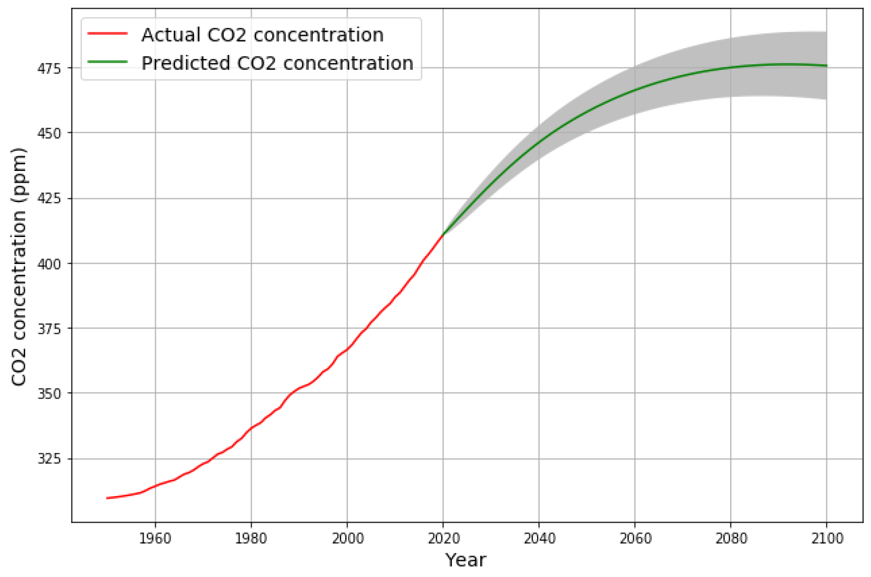
3.1. Prediction of 2021-2100 CO2 Concentration on the Basis of the 2021-2050 IEA Stated Policies Emission Scenario

To evaluate policy decisions, this model is applied to predict future CO₂ levels based on the – most conservative and most likely – Stated Polices Scenario of the IEA. This essentially means that the current energy consumption is continued, without significant further emission reductions beyond normal efficiency improvements. The Stated Policies Scenarios can be regarded as the most realistic prediction, because it is based on policies that are actually in effect.

This scenario assumes global emissions remain approximately at the current maximum of 37 Gt/yr = 4.6 ppm, with a slight reduction of 3% per decade. Total budget to 2100: 2640 Gt CO₂, then 29 Gt/yr (excluding land use change). The actually used data set for a realistic future projection is created by trend-extrapolating the stated policies beyond 2050 and assuming that the land use change data will follow the current trend and decrease to 0 by the year 2100 (Figure 7). Emissions will not be reduced to zero in the year 2100, but will approximately be at the 2005 level.

The prediction for the CO₂ concentration is based on the recursion of equation (11) with the parameter a=0.0165 and

C_{0}

= 245 ppm, derived from the constant relative absorption estimation of the 1950-2020 data, and hypothetical emission data from the discussed extended IEA scenario.

Figure 8 shows that the IEA stated policies scenario, i.e. no special CO₂ reduction policies, implies that a CO₂ concentration equilibrium of appr. 475 ppm will be reached during the second half of this century, with an 95% range of

[463, 488]

ppm. Based on the empirical CO₂ temperature proxy equation (6), this increase of the CO₂ concentration from 410 ppm (in 2020) to 475 ppm corresponds to a temperature increase of

{0.4}^{\circ}

C from 2020, or

{1.4}^{\circ}

C from 1850.

4. Conclusions

The model and results derived in this paper are based on very general assumptions:

The undeniable mass conservation of CO₂,
the assumption of approximate linearity of the relevant absorption processes w.r.t. CO₂ concentration . This assumption has been relaxed to allow for temperature dependent absorption,
the assumption that CO₂ concentration can be used as an upper limit proxy for temperature, i.e. a part of the temperature changes that can be explained by CO₂ concentration,
the assumption of constant natural emissions within the time period of measurement. We observed, however, apparent changes of natural emissions in the first half of the 20th century, resulting in a large prediction uncertainty. Further investigations are required for a better understanding, because these changes cannot be distinguished from land use changes, which also have a large uncertainty.

Although the model allows for varying absorptions over time, the data of the last 70 years, which is the period of the bulk anthropogenic CO₂ emissions, lead to the conclusion that relative CO₂ absorption has no significant temperature or other time dependent component, and a current CO₂ emission pulse is absorbed with a 42 year half life time.

The ex post validation of our model indicates that it predicts future CO₂ concentration very well on the basis of known emissions. In contrast, more than 40 years after their article was written, we see now that Oeschger’s complicated model, which explained the

C_{14}

content including bomb test data pretty well, failed badly for predicting future CO₂ levels. Their predicted 2020 additional CO₂ concentration beyond their assumed pre-industrial level of 295 ppm was more than 150% larger (590ppm = 295ppm + 295ppm) than the actual additional concentration (410ppm = 295ppm + 115ppm). It remains to be analyzed in detail whether the failure is due to overestimated emissions based on the unrealistic assumption of exponential emission growth, or whether it is caused by the model itself.

The main conclusion of this evaluation is, that for the most likely IEA emission scenario of approximately constant, slightly decreasing global emissions we can expect a maximum CO₂ concentration level of approximately 475 ppm in the second half of this century. At this point the emissions will be fully balanced by the absorptions, which is by definition the “net zero” situation.

Assuming the unlikely worst case that CO₂ concentration is fully responsible for all global temperature changes, the maximum expected rise of global temperature caused by the expected CO₂ concentration rise is

{0.4}^{\circ}

C from now or 1.4

{1.4}^{\circ}

C from the beginning of industrialisation.

Author Contributions

Conceptualization, John Reid and Joachim Dengler; methodology, Joachim Dengler; software, Joachim Dengler; validation, Joachim Dengler and John Reid; formal analysis, Joachim Dengler; writing—original draft preparation, Joachim Dengler; writing—review and editing, John Reid and Joachim Dengler; visualization, Joachim Dengler. All authors have read and agreed to the published version of the manuscript.

Data Availability Statement

All evaluations are based on publicly available data and software: Sea surface temperature data: https://www.metoffice.gov.uk/hadobs/hadsst2/diagnostics/global/nh+sh/monthly, CO₂ emissions, concentration, concentration growth, land use change: https://www.globalcarbonproject.org/carbonbudget/, https://www.icos-cp.eu/science-and-impact/global-carbon-budget/2022 Software: https://www.anaconda.com/products/distribution, Python modules matplotlib, pandas, statsmodels.

Acknowledgments

We thank Dr. Philipp Lengsfeld, re:look climate gGmbH Berlin for a critical reading of the manuscript. The publication of this work is partially funded by re:look climate gGmb Berlin.

Conflicts of Interest

The authors declare no conflict of interest.

Appendix A. Relation to the Bern Model

Our model relates to other papers that have been dealing with the relation between carbon emissions and CO₂ concentration. For the sake of clarity we separate the details of the relation to other concepts from the main thread of the paper.

The Bern model (Strassmann-2018) is a kind of accepted standard for climate science. We describe here how our model relates to the Bern model, and discuss the differences of respresentation.

Appendix A.1. Data Transformation of the Linear CO₂ Concentration Model

The foregoing considerations confirm that within the time range of the measurements

the linearity assumption of the absorptions and
the assumption of constant natural emissions

is reasonably valid. For showing the correspondence to the well-known Bern model (Strassmann-2018) we begin by using the temperature independent equation (8). We show how this maps to a single component of the Bern model. Eventually we show how the temperature dependent model maps to the multi component Bern model.

We transform the model in order to eliminate the assumed constant natural emissions by defining the “excessive CO₂ concentration”

C_{i}^{E}

caused by anthropogenic emissions

C_{i}^{E} = C_{i} - C_{0}

(A1)

and total anthropogenic emissions

E_{i}^{A}

by adding land use change to carbon emissions:

E_{i}^{A} = E_{i} + L_{i}

(A2)

With this substitution equation (8) becomes

C_{i}^{E} = E_{i}^{A} + C_{i - 1}^{E} - a \cdot C_{i - 1}^{E}

(A3)

C_{i}^{E} = E_{i}^{A} + (1 - a) \cdot C_{i - 1}^{E}

(A4)

This is the key equation to describe the relation between anthropogenic Emissions

E_{i}

and the resulting atmospheric excessive concentration. This relation explains why the “natural” pre-industrial CO₂ level of appr. 280 ppm is taken as the reference line and anthropogenic and natural emissions are treated separately.

In order to solve the equation analytically, i.e. describe the excessive concentratin as a function of the emissions we recursively substitute

C_{i - 1}^{E}

, starting with

C_{i}^{E} = E_{i}^{A} + (1 - a) \cdot (E_{i - 1}^{A} + (1 - a) \cdot C_{i - 2}^{E})

(A5)

Assuming

C_{i}^{E} = 0

and

E_{i} = 0

for

i < 0

, this sum is finite

C_{i}^{E} = \sum_{j = 0}^{i} {(1 - a)}^{j} \cdot E_{i - j}^{A}

(A6)

which is equivalent to

C_{i}^{E} = \sum_{j = 0}^{i} {(1 - a)}^{i - j} \cdot E_{j}^{A}

(A7)

Appendix A.1.1. Relation to the Impulse Response Model, the Carbon Cylce Component of the Bern Model

Equation (A7) says that any single unit carbon emission pulse (

E_{j} = δ (j))

will decay like a geometric series,

C_{i}^{P u l s e} = \sum_{j = 0}^{i} {(1 - a)}^{i - j} \cdot δ (j)

(A8)

C_{i}^{P u l s e} = {(1 - a)}^{i}

(A9)

For

a = 0.0165

the half life time

t_{0.5}

of a unit pulse is reached after

t_{0.5} = \frac{ln 0.5}{ln (1 - a)} \approx 42 (y e a r s)

(A10)

In order to show the correspondence of this model to the Impulse Response function of (Maier-Reimer-1987), we convert the discrete model to a continous model.

With

τ = \frac{1}{a}

we get

C_{i}^{E} = C_{i - 1}^{E} + E_{i}^{A} - \frac{C_{i - 1}^{E}}{τ}

(A11)

This is a discrete approximation of the differential equation

\frac{d C^{E} (t)}{d t} = E^{A} (t) - \frac{C^{E} (t)}{τ}

(A12)

This equation is solved by means of the Green’s function

G (t) = e^{- \frac{t}{τ}}

C^{E} (t) = \int_{0}^{t} G (t - t^{'}) \cdot E^{A} (t^{'}) d t^{'}

(A13)

C^{E} (t) = \int_{0}^{t} e^{- \frac{t - t^{'}}{τ}} \cdot E^{A} (t^{'}) d t^{'}

(A14)

This gives

τ

the meaning of a time constant in an exponential decay. Approximating equation (A14) with discrete samples is the sum

C_{i}^{E} = \sum_{j = 0}^{i} e^{- \frac{i - j^{'}}{τ}} \cdot E_{j}^{A}

(A15)

This is equivalent to equation (A7) with the approximation

l n (1 - a) = ln (1 - \frac{1}{τ}) \approx \frac{1}{τ}

which is valid for

a < 0.1

We will now show that this is formally equivalent to the full Bern model, where the general form of the impulse response function (IRF) is (Strassmann-2018, Equation (19)):

G^{H} = A_{0} + \sum_{j = 1}^{N} A_{j} \cdot e^{- \frac{t}{τ_{j}}}

(A16)

with the constraint

\sum_{j = 0}^{N} A_{j} = 1

(A17)

The correspondence can best be seen when we start with the differential form of the pulse response equation (Strassmann-2018, Equation (21), variables renamed). Instead of the infinitely long time constant we assume a very large one, so all terms can be written in the same form

\frac{d C_{k}^{E}}{d t} = E^{A} (t) \cdot A_{k} - \frac{C_{k}^{E}}{τ_{k}}

(A18)

with

\sum_{k = 0}^{N} A_{k} = 1

(A19)

and

\sum_{k = 0}^{N} C_{k} (t) = C^{E} (t)

(A20)

When we substitute

a_{k} (t) = \frac{C_{k} (t)}{τ \cdot C^{E} (t)}

we get

\frac{d C_{k}}{d t} = E^{A} (t) \cdot A_{k} - a_{k} (t) \cdot C^{E} (t)

(A21)

and with (30) and (31)

\frac{d C^{E}}{d t} = E^{A} (t) - \sum_{k = 0}^{N} a_{k} (t) \cdot C^{E} (t)

(A22)

Apart from the time dependence of

a (t)

this is identical to Equation (24) with

a (t) = \sum_{k = 0}^{N} a_{k} (t)

(A23)

With these transformations we have shown that the IRFs of the Bern model can be mapped to a simple univariate model with a time varying coupling variable. The time dependency of the coupling variable

a (t)

creates the nonlinearity which Strassmann and Joos (Strassmann-2018, chapter 2) talk about. The simplest possible time dependence of a is a linear time dependence which can easily and in a statistically robust way be tested by testing for a linear trend in a:

a (t) = a_{0} + a_{1} \cdot t

(A24)

Time dependence of absorption is not directly physically meaningful, at best it is a proxy for other physical processes that are time dependent. Looking at the short time ranges where measurements are available, changes caused by temperature are the most relevant. Therefore replacing the time dependence by temperature dependence is a meaningful heuristics.

Appendix A.2. Discussion of the Paper from Weber, Lüdecke and Weiss

The paper “A simple model of the anthropogenically forced CO₂ cycle” [7] also applies a linear model, but separates the oceanic and biospheric contribution. Their Equation (3) can be related to our equation (8) in combination with our equation (4), where their yearly emissions are noted with

\bar{n_{t o t} (t)}

(

E_{i}

L_{i}

in our model), with the difference, that their biospheric absorption

n_{b} (t)

is not considered to be proportional to the CO₂ concentration

N_{a}

(t) (=

C_{i}

in our model) as in our model, but to its concentration growth

n_{a}

(t) (=

C_{i}

C_{i - 1}

in our model). The behaviour of

C_{3}

as well as

C_{4}

plants clearly indicate that the absorption is proportional to the absolute CO₂ concentration within the relevant CO₂ concentration range of 280..600 ppm. The main problem of the different definitions of oceanic and biospheric absorption is that it is not possible to easily merge the different processes for the determination of the global CO₂ retention time. Contrary to this in our model all individual absorption constants add up to the total absorption constant. We question the physical meaning of the subsequent denominator (1+b) in their Equation (7). Intuitively we would expect another sink to increase the difference between emissions and oceanic absorption, and not make it smaller as in their Equation (7). This may explain the discrepancy between our time constant of 42 years and theirs of 100 years.

Another difference of their approach to ours is that they estimate the 2 absorption constants (equations (8) and (9) in their paper) completely unrelated from their main Equation (7), which leads to the strange phenomenon, that their main Equation (7) does not contain any free parameters. This raises the question of how the system is able to react to changing emission scenarios. In our understanding

N_{a} (t)

should be a measured input variable in the phase of parameter estimation, whereas in their Equation (7)

N_{a}

(t) appears to be the unknown output variable.

Appendix A.3. Discussion of Harde’s Paper and Its Critics

Equation (A4) is formally identical to equation 11 in Harde’s publication "Scrutinizing the carbon cycle and CO₂ residence time in the atmosphere" [16]. His paper as a whole and in particular this formula have been heavily criticised [17]. This makes it necessary to discuss some issues raised in this discussion. Formally the criticism that one equation is not enough to describe the CO₂ concentration in the atmosphere (“1-box model”) as a function of emissions is not justified, because

the mass conservation of CO₂ can hardly be disputed, see equation (1),
the linear dependence of absorption from concentration (equation (3)) has been extensively discussed above, and the deviations from this assumption in the measured data are so statistically insignificant, that it is not justified to dismiss a model assuming constant a.
the assumption of a state of equilibrium between natural emissions and absorptions (equation (7)) during recent pre-industrial centuries is in my understanding scientific consensus (paleo-climate and its CO₂ variability is not the issue here), and most mainstream publications explicitely or implicitely assume a constant pre-industrial CO₂ concentration of appr. 280 ppm.
given the measured anthropogenic emissions as well as the measured CO₂ concentrations, the equation is well-posed and therefore can be solved without further other equations,
the remaining small residual errors have been recognized and discussed as being caused by e.g. the El Nino southern oscillation and vulcanic eruptions [6], the systematic deviations in the first part of the 20th century remain to be fully evaluated.

Harde’s approach to solve the equation in question is flawed, however. He claims the total anthropogenic and natural emissions to be 97.2 ppm/yr, most of which are assumed to be natural emissions. Contrary to his assumption, the data from 1950 to 2020 force us to the conclusion that the yearly net natural emissions are 4.0 ppm (95% interval is [3.7,4.4]), which are fully compensated by absorption. Obviously the total amount of emitted and absorbed CO₂ is much larger, but all emissions, which are compensated by daily or seasonal absorptions, i.e. within the year, are invisible in the yearly balance and do not count for the emission/concentration relation.

Therefore, the anthropogenic emissions are indeed a key control knob of the resulting excess CO₂ concentration in the atmosphere, but the data lead us to a relatively short half life time of appr. 42 years with no “eternal” CO₂ remaining beyond the natural equilibrium level.

References

Siegenthaler, U.; Oeschger, H. Predicting Future Atmospheric Carbon Dioxide Levels: The predictions provide a basis for evaluating the possible impact of the continuing use of fossil fuel. Science 1978, 199, 388–395. [Google Scholar] [CrossRef] [PubMed]
Maier-Reimer, E.; Hasselmann, K. Transport and storage of CO2 in the ocean – an inorganic ocean-circulation carbon cycle model. Climate dynamics 1987, 2, 63–90. [Google Scholar] [CrossRef]
Joos, F.; Roth, R.; Fuglestvedt, J.S.; Peters, G.P.; Enting, I.G.; Von Bloh, W.; Brovkin, V.; Burke, E.J.; Eby, M.; Edwards, N.R.; et al. Carbon dioxide and climate impulse response functions for the computation of greenhouse gas metrics: a multi-model analysis. Atmospheric Chemistry and Physics 2013, 13, 2793–2825. [Google Scholar] [CrossRef]
Strassmann, K.M.; Joos, F. The Bern Simple Climate Model (BernSCM) v1. 0: an extensible and fully documented open-source re-implementation of the Bern reduced-form model for global carbon cycle–climate simulations. Geoscientific Model Development 2018, 11, 1887–1908. [Google Scholar] [CrossRef]
Halparin, A. Simple Equation of Multi-Decadal Atmospheric Carbon Concentration Change 2015.
Spencer, R. Spencer, R. A simple model of the atmospheric CO2 budget 2019.
Weber, W.; Lüdecke, H.J.; Weiss, C. A simple model of the anthropogenically forced CO 2 cycle. Earth System Dynamics Discussions 2015, 6, 2043–2062. [Google Scholar]
Friedlingstein, P.; Jones, M.W.; O’Sullivan, M.; Andrew, R.M.; Bakker, D.C.; Hauck, J.; Le Quéré, C.; Peters, G.P.; Peters, W.; Pongratz, J.; et al. Global carbon budget 2021. Earth System Science Data 2022, 14, 1917–2005. [Google Scholar] [CrossRef]
Hausfather, Z. Global CO2 Emissions Have Been Flat for a Decade, New Data Reveals. Carbon Brief; 2021. https://www.carbonbrief.org/global-co2-emissions-have-been-flat-for-a-decade-new-data-reveals, 2021.
IEA. World Energy Outlook, Scenario trajectories and temperature outcome 2021.
Duffy, K.A.; Schwalm, C.R.; Arcus, V.L.; Koch, G.W.; Liang, L.L.; Schipper, L.A. How close are we to the temperature tipping point of the terrestrial biosphere? Science Advances 2021, 7, eaay1052. [Google Scholar] [CrossRef] [PubMed]
Watson, A.J.; Schuster, U.; Shutler, J.D.; Holding, T.; Ashton, I.G.; Landschützer, P.; Woolf, D.K.; Goddijn-Murphy, L. Revised estimates of ocean-atmosphere CO2 flux are consistent with ocean carbon inventory. Nature communications 2020, 11, 1–6. [Google Scholar] [CrossRef]
Oeschger, H.; Siegenthaler, U.; Schotterer, U.; Gugelmann, A. A box diffusion model to study the carbon dioxide exchange in nature. Tellus 1975, 27, 168–192. [Google Scholar] [CrossRef]
HadSST2. HadSST2 - Met Office sea surface temperature anomalies monthly data, 1850-2013 2013.
Herman, J.; DeLand, M.; Huang, L.K.; Labow, G.; Larko, D.; Lloyd, S.; Mao, J.; Qin, W.; Weaver, C. A net decrease in the Earth’s cloud, aerosol, and surface 340 nm reflectivity during the past 33 yr (1979–2011). Atmospheric Chemistry and Physics 2013, 13, 8505–8524. [Google Scholar] [CrossRef]
Harde, H. Scrutinizing the carbon cycle and CO2 residence time in the atmosphere. Global and Planetary Change 2017, 152, 19–26. [Google Scholar] [CrossRef]
Köhler, P.; Hauck, J.; Völker, C.; Wolf-Gladrow, D.; Butzin, M.; Halpern, J.; Rice, K.; Zeebe, R. Comment on S̎crutinizing the carbon cycle and CO2 residence time in the atmosphere. Global and Planetary Change, 2018; 164, 67–71. [Google Scholar]

Figure 1. Emissions, land use change, and CO₂ concentration change

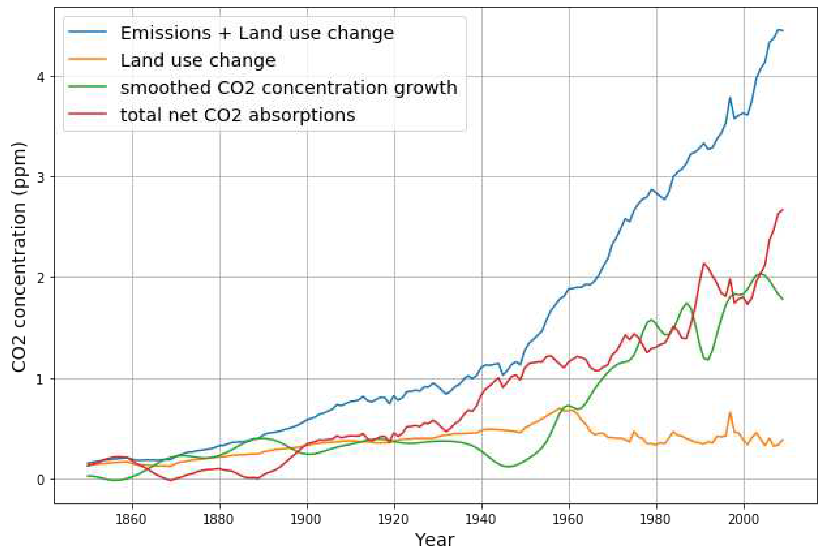
Figure 2. Effective absorption vs CO₂ concentration

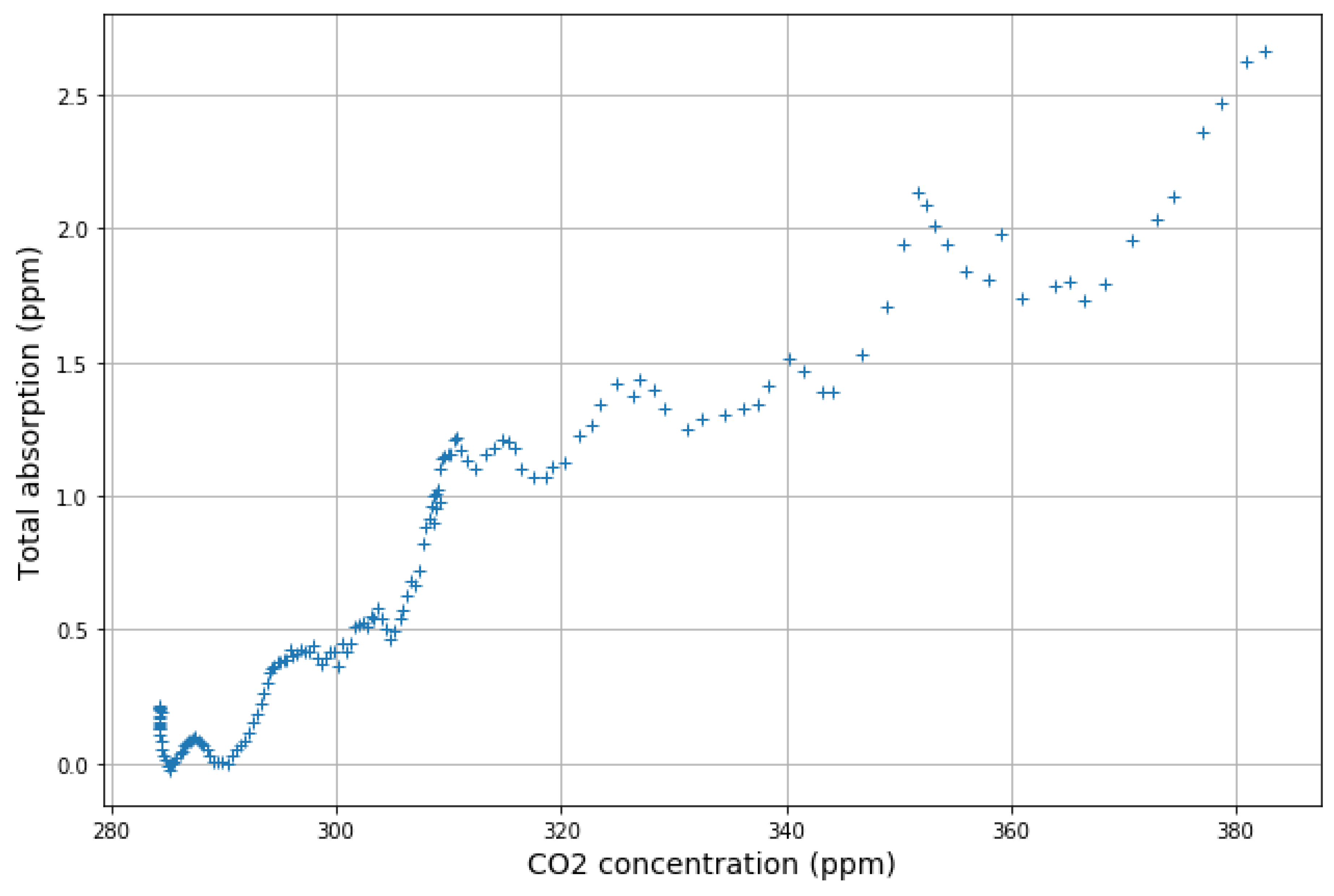
Figure 3. CO₂ concentration as a proxy for global temperature

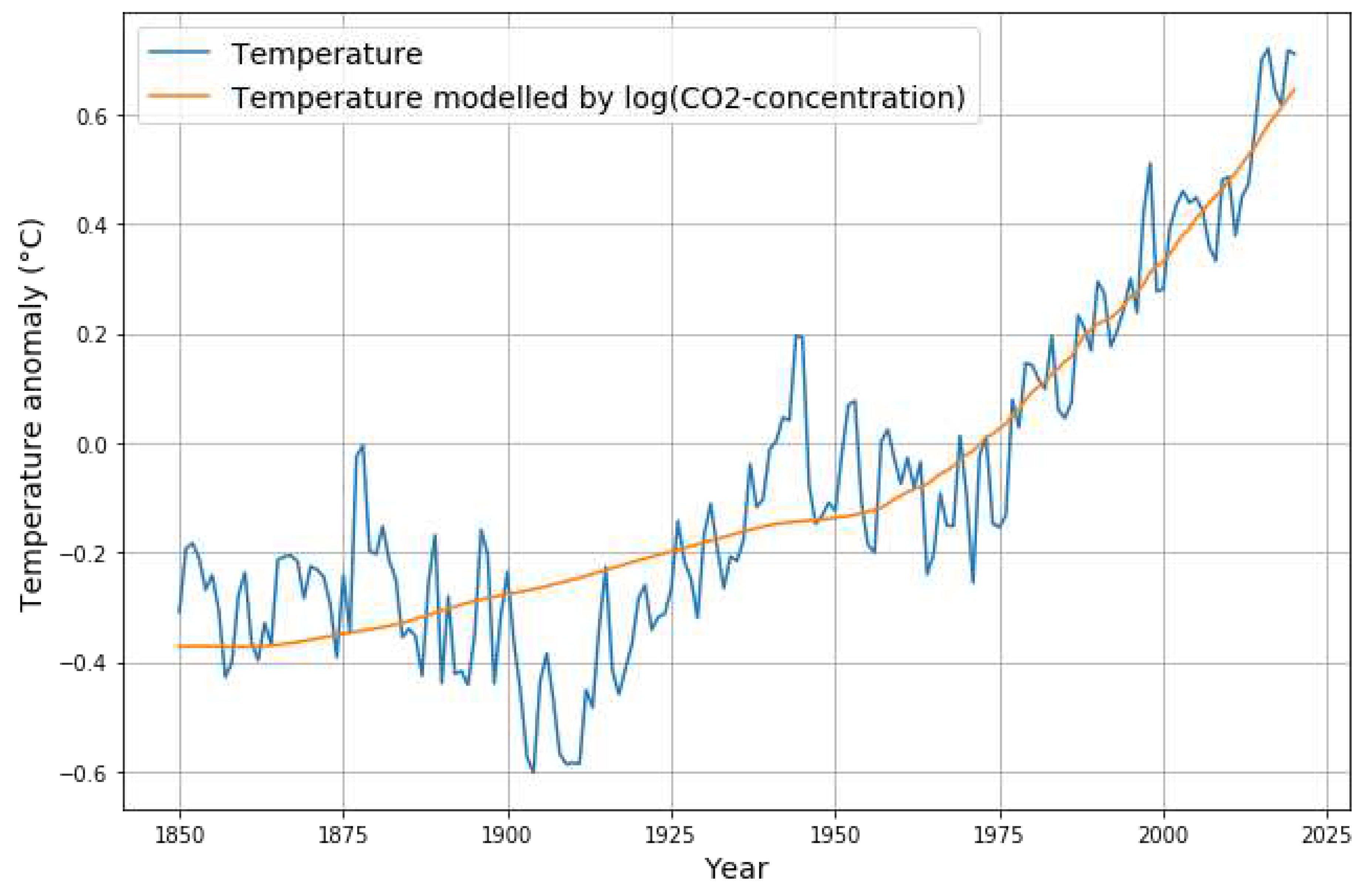
Figure 4. Linear model of CO₂ absorption

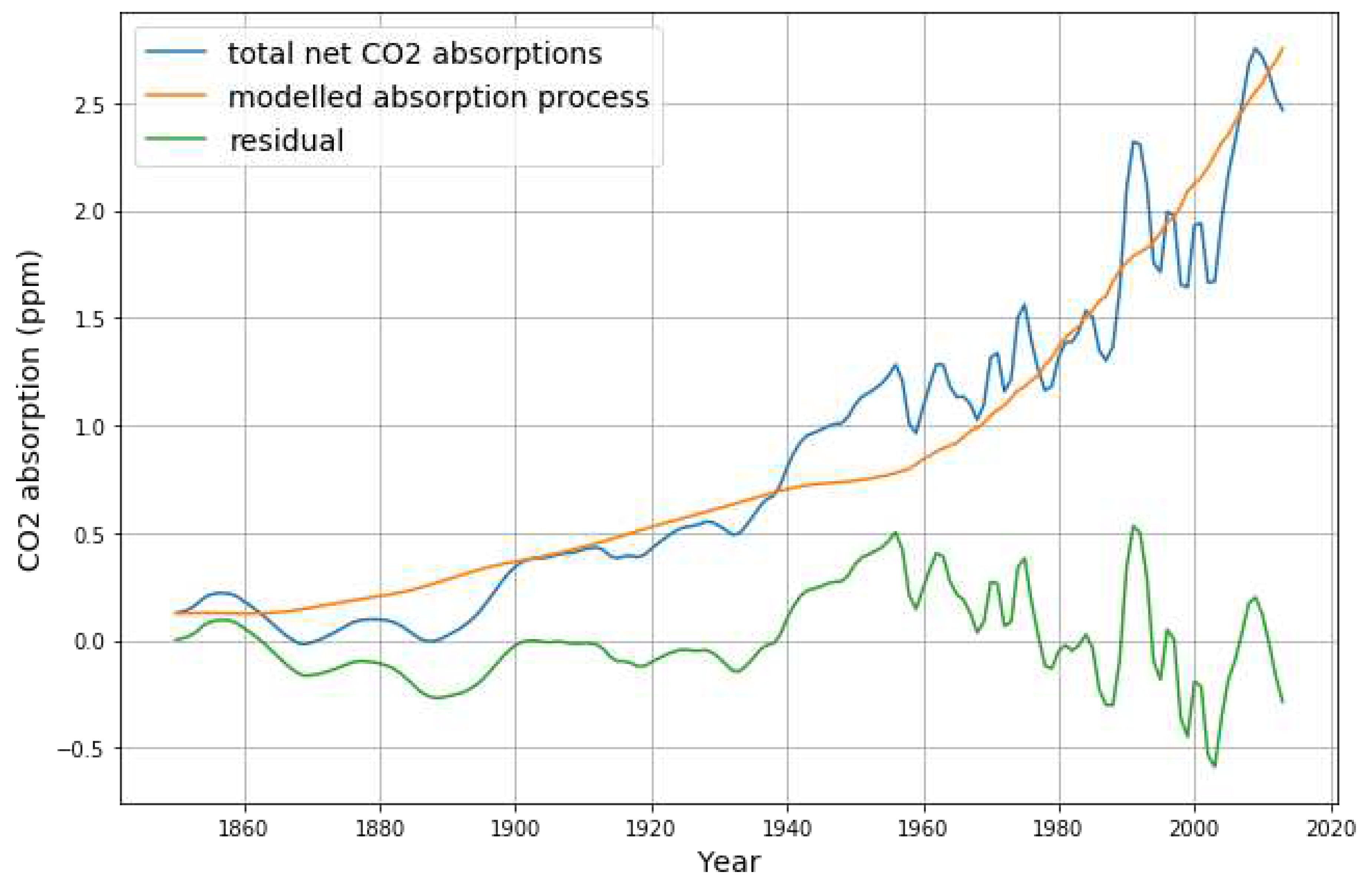
Figure 5. Comparing absorption models 1950-2000

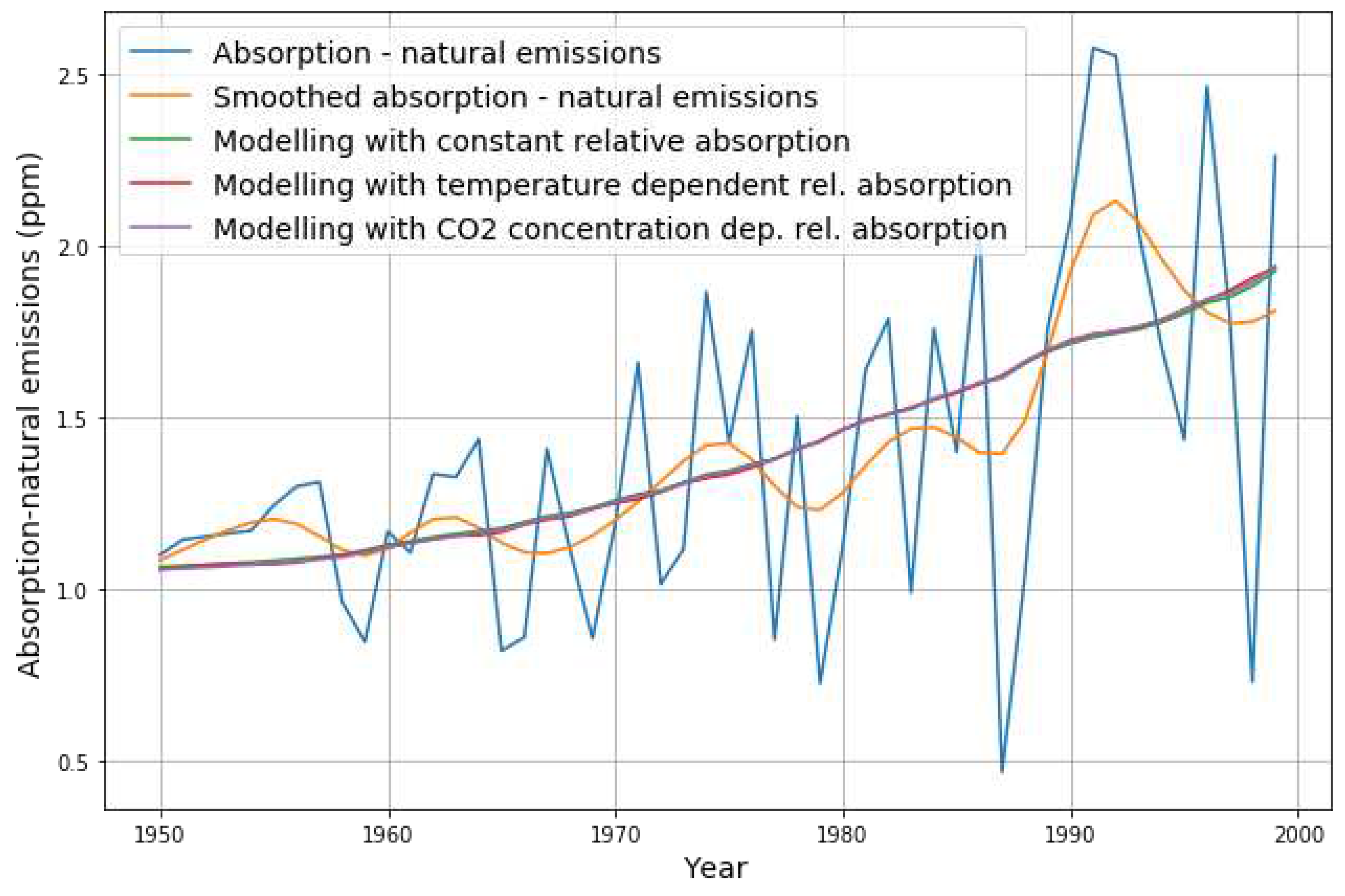
Figure 6. Actual (1950-2020) and predicted (2000-2020) CO₂ concentration

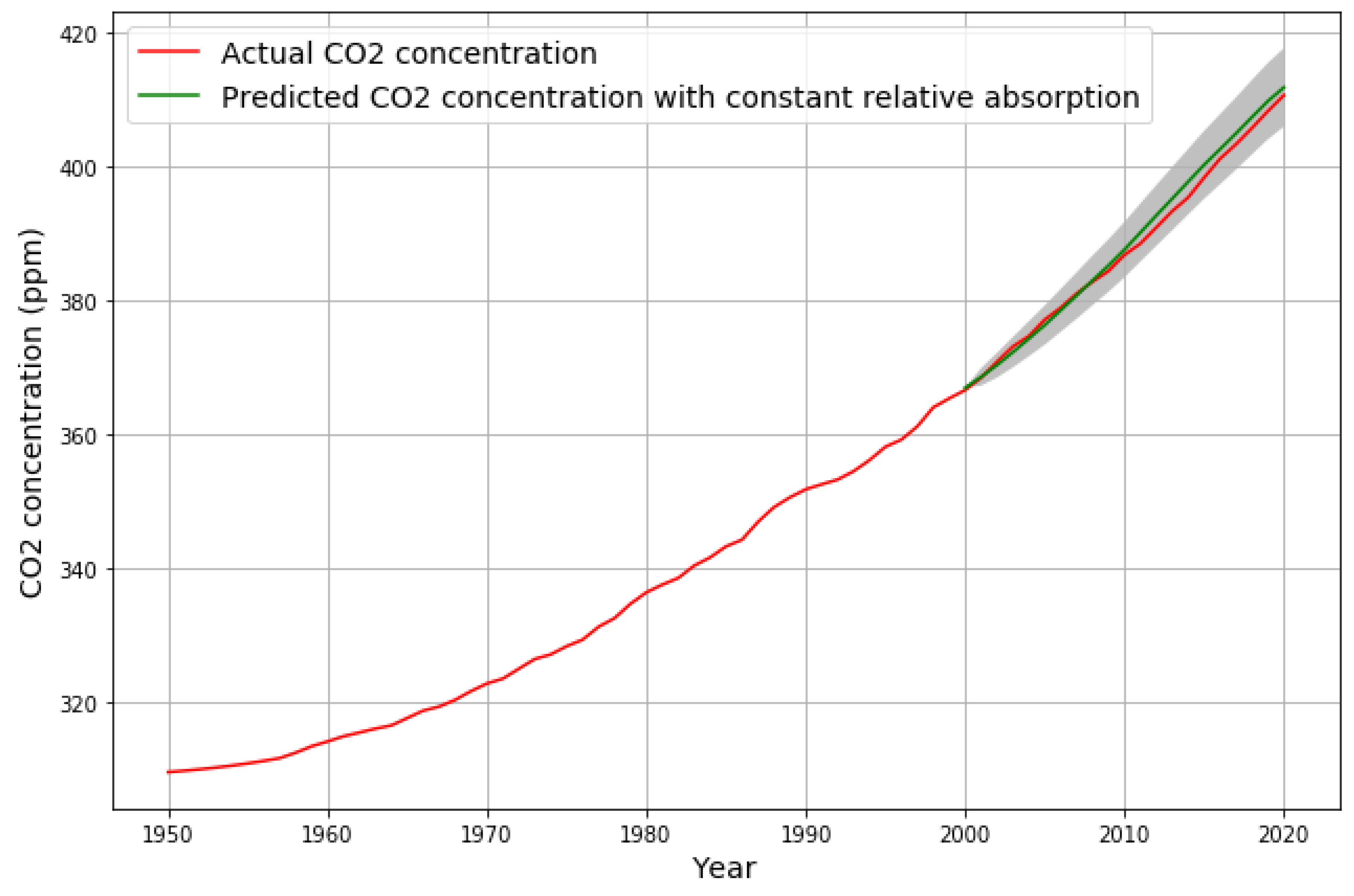
Figure 7. Emissions 1950-2020, IEA emission scenario 2021-2050, and extension to 2100

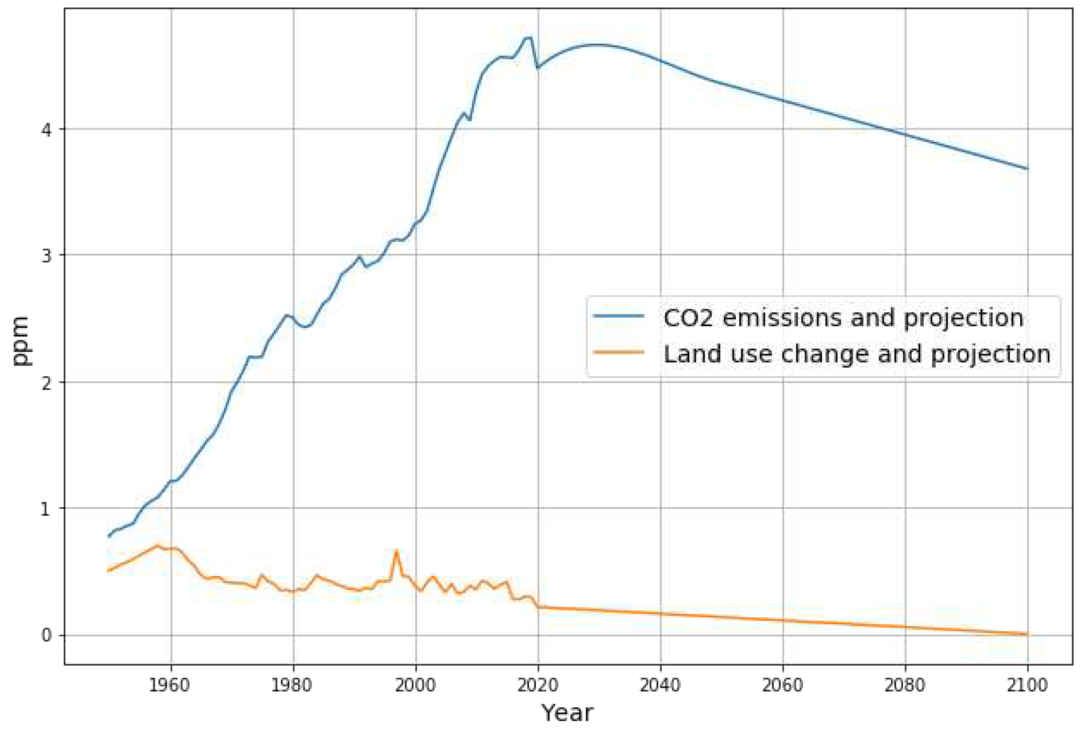
Figure 8. Actual (1950-2020) and predicted (2021-2100) CO2 concentration for IEA stated policies scenario.

Disclaimer/Publisher’s Note: The statements, opinions and data contained in all publications are solely those of the individual author(s) and contributor(s) and not of MDPI and/or the editor(s). MDPI and/or the editor(s) disclaim responsibility for any injury to people or property resulting from any ideas, methods, instructions or products referred to in the content.

© 2023 by the authors. Licensee MDPI, Basel, Switzerland. This article is an open access article distributed under the terms and conditions of the Creative Commons Attribution (CC BY) license (http://creativecommons.org/licenses/by/4.0/).

Copyright: This open access article is published under a Creative Commons CC BY 4.0 license, which permit the free download, distribution, and reuse, provided that the author and preprint are cited in any reuse.

MDPI Initiatives

Important Links

Choose an area of interest and we will send you notifications of new preprints at your preferred frequency.

Disclaimer