An Efficient Gaussian Mixture Model and It's Application to Neural Network

Weiguo Lu; Deng Ding; Fengyan Wu; Gangnan Yuan

doi:10.20944/preprints202302.0275.v1

Preprint

Article

An Efficient Gaussian Mixture Model and It's Application to Neural Network

This version is not peer-reviewed.

Weiguo Lu

Deng Ding,Fengyan Wu,

Gangnan Yuan^*

Weiguo Lu

Deng Ding,Fengyan Wu,

Gangnan Yuan^*

This version is not peer-reviewed.

Downloads

497

Views

211

Comments

Submitted:

15 February 2023

Posted:

16 February 2023

Read the latest preprint version here

A peer-reviewed article of this preprint also exists.

Abstract

While modeling data in reality, uncertainties in both data (aleatoric) and model (epistemic) are not necessarily Gaussian. The uncertainties could appear with multimodality or any other particular forms which need to be captured. Gaussian mixture models (GMMs) are powerful tools that allow us to capture those features from a unknown density with a peculiar shape. Inspired by Fourier expansion, we propose a GMM model structure to decompose arbitrary unknown densities and prove the property of convergence. A simple learning method is introduced to learn GMMs through sampled datasets. We applied GMMs as well as our learning method to two classic neural network applications. The first one is learning encoder output of autoencoder as GMMs for handwritten digits images generation. The another one is learning gram matrices as GMMs for style-transfer algorithm. Comparing with the classic Expectation maximization (EM) algorithm, our method does not involve complex formulations and is capable of achieving applicable accuracy.

Keywords:

Neural Network

;

Uncertainties

;

GMM

;

Density approximation

Subject:

Computer Science and Mathematics - Computer Science

1. Introduction

Gaussian Mixture Models (GMMs) are powerful, parametric, and flexible models in the probabilistic realm. GMMs tackle two important problems. The first is known as the “inverse problem,” in which

f^{- 1} (x)

and x are not unique one-to-one mappings [1]. The second issue is the uncertainty problem of both the data (aleatoric) and the model (epistemic) [2,3,4]. When we consider the two problems together, it is easy to see that if we deal with multimodal problems, classic model assumptions start falling apart. Traditionally, we attempt to discover the relationship between input x and output y, which is denoted as

y = f (x) + ϵ

with erro

ϵ

.In a probabilistic sense, the above model assumption is equivalent to

y \sim Normal (f (x), σ)

. In terms of inverse and uncertainty problems, the model assumption is

y \sim UnkownDistribution (θ (x))

. Under this condition, when y is no longer following any distribution in a known form, GMM becomes a viable option for model data. If

y \sim UnkownDistribution (θ (x)) \approx G M M (f (x))

could be satisfied, then we could use GMM as a general model regardless of whatever distribution y is following. The question remaining for us to answer is whether GMMs can approximate arbitrary densities. Some studies show that all normal mixture densities are dense in the set of all density functions under the

L 1

metric [5,6,7]. A model that can fit an arbitrary distribution density is relatively similar, as it requires the model to imitate all possible shapes of distribution density. In this work, taking ideas from Fourier expansion, we assume that any distribution density can be approximately seen as a combination with a set of finite Gaussian distributions. To put it another way, any density can be approximated by a set of Gaussian distribution bases with fixed means and variances. GMM approximates an unknown density by using data to learn the amplitudes (coefficients) of the Gaussian components.In summary, we have X as input data,

Y \sim {UnknownDistribution}_{y} = G_{y}

as output data, and

G M M (f (x)) + ϵ \approx G_{y},

here

f (x)

is the function that requires learning. To learn

f (x)

, which maps input x into GMM parameters, we can use any modeling technique.

While modeling using GMM, we need to perform two stages of learning. To begin, we must find appropriate GMM parameters to approximate the target distribution

G_{y}

. Secondly, once we have the values of GMM parameters

θ

, we can learn model

f (x)

map to

θ

. In this paper, we mainly discuss the first part of learning. How to learn a GMM to approximate the target distribution. Fitting a GMM from the observed data related to two problems: 1) how many mixture components are needed; 2) how to estimate the parameters of the mixture components.

For the first problem, some techniques are introduced [5]. For the second problem, as early as 1977, the Expectation Maximization (EM) algorithm [8] was well developed and capable of fitting GMMs based on minimizing the negative log-likelihood (NLL). While the EM algorithm remains one of the most popular choices for learning GMMs, other methods have also been developed for learning GMMs [9,10,11]. The EM algorithm has a few drawbacks. Srebro [12] asked an open question that questioned the existence of local maxima between an arbitrary distribution and a GMM. That paper also addressed the possibility that the KL-divergence between an arbitrary distribution and mixture models may have non-global local minima. Especially in cases where the target distribution has more than k components but we fit it with a GMM with fewer than k components. Améndola at al. [13] has shown that the likelihood function for GMMs is transcendental. Jin et al. [14] resolved the problem that Srebro discovered and proved that with random initialization, the EM algorithm will converge to a bad critical point with high probability. The maximum likelihood function is transcendental and will cause arbitrarily many critical points. Intuitively speaking, when handling any distribution with multimodal analysis, if the size of the GMM components is less than the peaks that the target distribution contains, it will lead to an undesirable estimation.

Furthermore, instead of a bell shape, if a peak of the target distribution is present as a flat top like a roof, a single Gaussian component is limited in capturing these kinds of features and is not capable of making a good estimation. It is not a surprise that the likelihood function could have bad local maxima and be arbitrarily worse than any global optimum. Other studies turn their heads to the Wasserstein distance. Instead of minimizing the NLL function or Kullback-Leibler divergence, Wasserstein distances are introduced to replace the NLL function [11,15,16]. These methods avoid the downside of using NLL, but the calculation and formulation of the learning process are relatively complex.

Instead of following the EM algorithm, we take a different path. The main concept of our work is to take the idea of Fourier expansion and apply it to density decomposition. Similarly, like Fourier expansion, our model needs a set of base components, and their location is predetermined. Instead of using a couple of components, we use a relatively large number of components to construct this base. The benefit of this approach is that these bases represent how much detail our models can capture without going into a calculation process to decide how many GMM components are needed. Another benefit of this idea is that, on a predetermined basis, the learning parameters become relatively simple. We only need to learn an appropriate set of

π

which are the probability coefficients of normal components, to reach an optimum approximation. A simple algorithm without heavy formulation is designed to achieve this task. More detailed explanations, formulations, and proofs are provided in the next section. It is worth mentioning that, like cousin expansion, if base frequencies are not enough, there will be information loss for the target sequence. This method suffers similar information losses from not enough Gaussian components. We provide a measurement of the information loss. In our experiments, our method provided a good estimation result.

GMMs have been used across computer vision and pattern classification among many others [17,18,19,20]. Additionally, GMMs can also be used to learn embedded space in neural networks [11]. Similarly, as Kolouri et al., we apply our algorithm to learn embedded space in neural networks in two classic neural network applications of handwritten digits generation using autoencoders [21,22] and style transfer [23]. This helps us turn latent variables into a complex distribution, which allows us to perform sampling to create variation. More detail is provided in Section 4.

Section 2 introduces Fourier expansion-inspired Gaussian mixture models, shows this method is capable of approximating arbitrary densities, discusses the convergency, defines a suitable metric, and details some of its properties. Section 3 provides our methodology for fitting a GMM through data, introduces two learning algorithms, and shows learning accuracy through experiments. Section 4 presents two neural network applications. The final section provides a summary and conclusions.

2. Decompose Arbitrary Density by GMM

In this section, we show our method from scratch, including learning algorithms, as well as prove that the idea of density decomposition by GMM is feasible with bounded approximation error. A metric called density information loss is introduced to measure the approximation error between target density and GMM. Let’s begin with the basic assumption and notation:

Observed a dataset X, which is following a unknown distribution with density $f (x)$ ;
Assuming there is a GMM that matches the distribution of X : $f (x) \approx g (x) + ϵ$ ;
The density of GMM: $g (x) = \sum_{n} π_{i} ϕ_{i} (x)$ ;
As general definition of GMM, $\sum_{n} {\tilde{π}}_{i} = 1$ and $ϕ_{i} (x) \sim N (μ_{i}, σ_{i})$ .

In this work, we mainly discuss one-dimensional cases. The GMM is mixed with Gaussian distributions rather than multivariate Gaussian distributions.

2.1. General Concept of GMM Decomposition

The idea behind GMM decomposition is a Fourier series in probability that, assuming arbitrary density, can be accurately decomposed by infinite mixtures of Gaussian distributions. As mentioned earlier, a lot of studies prove that the likelihood of GMM has many critical points. There are far too many sets of

π, μ

and

σ

that could produce the same likelihood result on a given dataset. Learning three sets of parameters,

π, μ, σ

could increase the complexity of the learning process. Not to mention that these parameters interact with each other. Changing one of them could lead to new sets of optimal solutions for others. If we consider that GMM can decompose any density like the Fourier series into a periodic sequence, we can predetermine the base Gaussian distributions (component distributions).

In practice,

μ

can be set to be evenly spread out though the dataset space. The parameter

σ

can be treated as a hyperparameter that adjusts overall GMM density smoothness. This means that

μ, σ

of the component distribution are non-parametric and do not need to be optimised. The parameter

π

is the only remaining problem for us to solve. Our goal shifted from finding the best set of

π, m u, σ

to finding the best set of

π

on a given dataset. With this idea, our GMM set-up becomes:

$g (x) = \sum_{n} π_{i} ϕ_{i} (x)$ is the density of GMM;
$\sum_{n} π_{i} = 1$ , $ϕ_{i} (x) \sim N (μ_{i}, σ)$ , n is the numbers of normal distributions;
$r = \frac{m a x (X) - m i n (X)}{n}$ is the interval for locating $μ_{i}$ ;
$μ_{i} = m i n (X) + i \times r$ are means for Gaussian components;
$σ = t \times r$ is——;
t is a real number hyper-parameter, usually $1 \leq t \leq 5$ .

2.2. Approximate Arbitrary Density by GMM

In this subsection, we show that, in certain conditions, if the component size of a mixture Gaussian model goes to infinite, the error of approximating an arbitrary density can go toward zero.

Through the idea of Monte Carlo, we could assume that the accuracy of a fine frequency distribution estimation of the target probability mass through dataset is good enough in general. A frequency distribution could also be seen as a mixture distribution with a uniform distribution components. Elaborate from this, if we swap each uniform distribution into a Gaussian unit and push this toward infinite, we could have a correct probability mass approximation of any target distribution. Because we do not have access to the true density, the dataset is all we have, an accurate probability mass is generally good enough in practice. Let

ω_{i} = \{x \in (μ_{i} - r, μ_{i} + r]\}

, we have:

\begin{matrix} [\begin{matrix} \int_{ω_{0}} g (x) d x \\ . \\ . \\ . \\ \int_{ω_{n}} g (x) d x \end{matrix}] = [\begin{matrix} P_{g} \{ω_{0}\} \\ . \\ . \\ . \\ P_{g} \{ω_{n}\} \end{matrix}] \approx [\begin{matrix} P_{f} \{ω_{0}\} \\ . \\ . \\ . \\ P_{f} \{ω_{n}\} \end{matrix}] = [\begin{matrix} \int_{ω_{0}} f (x) d x \\ . \\ . \\ . \\ \int_{ω_{n}} f (x) d x \end{matrix}] . \end{matrix}

Expand the density of GMM

g (x)

results

[\begin{matrix} \int_{ω_{0}} ϕ_{0} (x) d x & . & . & . \int_{ω_{0}} ϕ_{n} (x) d x \\ ⋮ & ⋮ & ⋮ & ⋮ \\ \int_{ω_{n}} ϕ_{0} (x) d x & . & . & . \int_{ω_{n}} ϕ_{n} (x) d x \end{matrix}] [\begin{matrix} π_{0} \\ ⋮ \\ π_{n} \end{matrix}] = [\begin{matrix} P_{g} \{ω_{0}\} \\ ⋮ \\ P_{g} \{ω_{n}\} \end{matrix}]

It is not hard to notice that, if

\int_{ω_{i}} ϕ_{i} (x) d x \approx 1

which means that each Gaussian component is very dense in their region, GMM become a discrete distribution that can be precisely 1:1 clone the estimation probability mass. It becomes:

[\begin{matrix} 1 & . & . & . 0 \\ ⋮ & ⋮ & ⋮ & ⋮ \\ 0 & . & . & . 1 \end{matrix}] [\begin{matrix} π_{0} \\ ⋮ \\ π_{n} \end{matrix}] \approx [\begin{matrix} P_{g} \{ω_{0}\} \\ ⋮ \\ P_{g} \{ω_{n}\} \end{matrix}] \approx [\begin{matrix} P_{f} \{ω_{0}\} \\ ⋮ \\ P_{f} \{ω_{n}\} \end{matrix}]

These simple deductions say that under this set up, a GMM with a large size of component is guaranteed to perform as well as a frequency distribution. Furthermore, changing the mixture component from a regular Gaussian distribution to a truncated normal distribution or uniform distribution could lead to the same conclusion. One good thing about this set up is that it could bring discrete probability mass estimation to continuous density. Allow us to deal with regression problems in a classification manner. We do suffer loss of information at some points in the density, but generally, in practice, the probability mass is what we are looking for. For example, let’s say we are trying to figure out the distribution of people’s height. Instead of looking for a precise density estimation of people’s height,

f \{h e i g h t = 1.801 m\}

P \{1.80 m \leq h e i g h t \leq 1.81 m\}

is what we targeting. Therefore, if we accept a discrete frequency distribution as one of our general approximation models, there is no reason that GMM can not be used to approximate arbitrary density, because it is capable of performing as good as frequency distribution estimation.

2.3. Density Information Loss

Even though GMM can approximate arbitrary density similarly to frequency distribution, density information within

ω

remains a problem that needs to be discussed. In another word, even if we learn a model that probability mass is equal to target density

P_{g} \{ω\} = P_{f} \{ω\}

, the differentiation is not equal

\frac{d P_{g} \{ω\}}{d x} \neq \frac{d P_{f} \{ω\}}{d x}

. We could apply KL-divergence or Wasserstain distance to measure the difference between two densities. But in our set up, we introduce a simple metric to measure regional density information loss (DIL). If DIL is small enough under some conditions, then we may be able to conclude that GMM can be a generalised model to decompose arbitrary density.

First of all, assume we have already learned a GMM which achieves that probability mass is correctly mapped to the target distribution. We split the data space into n regions denoted as

ω_{i}

the same as Section 2.3.

[\begin{matrix} P_{g} \{ω_{0}\} \\ ⋮ \\ P_{g} \{ω_{n}\} \end{matrix}] \approx [\begin{matrix} P_{f} \{ω_{0}\} \\ ⋮ \\ P_{f} \{ω_{n}\} \end{matrix}]

The total density information loss is sum of absolute error.

\begin{matrix} D I L = \sum_{i = 1}^{n} \int_{ω_{i}} | f (x) - g (x) | d x \end{matrix}

Because the integration is not particularly easy for us to calculate, here we divide

ω_{i}

further into m smaller regions to estimate DIL.

\begin{matrix} \sum_{k = 1}^{m} d_{k} = ω_{i}, \\ D I L \approx \sum_{i = 1}^{n} \sum_{j = 1}^{m} \int_{d_{i j}} | f (x) - g (x) | d x \approx \sum_{i = 1}^{n} \sum_{j = 1}^{m} | P_{f} \{d_{i j}\} - P_{g} \{d_{i j}\} |, \end{matrix}

Denote that:

L (ω_{i}) = \sum_{j = 1}^{m} | P_{f} \{d_{i j}\} - P_{g} \{d_{i j}\} |

(1)

Where

L (ω_{i})

is the discrete approximation of density information loss within region

ω_{i}

. If

L (ω_{i})

is universally bounded in some conditions for all

ω

, the overall DIL is bounded. For any

x_{i j}

from

ω_{i}

, if

\begin{matrix} | P_{f} \{x_{i j} \pm d\} - P_{g} \{x_{i j} \pm d\} | \leq τ_{i} \leq τ, \end{matrix}

we have

\begin{matrix} D I L \leq n * m * τ . \end{matrix}

In fact,

L (ω_{i})

is bound within a comfortable condition. In Figure 1, the plot demonstrates the density of target distribution(blue) and GMM(red) in a small region

ω_{i}

. The probability

P_{f} \{ω_{i}\}

is equal to

P_{g} \{ω_{i}\}

. Evenly split

ω_{i}

into 4 smaller areas and each area has length d. When we look at this geometrical relationship between target distribution

f (x)

and GMM

g (x)

, we discover that for each small region d,

| P_{f} \{d_{j}\} - P_{g} \{d_{j}\} |

is bounded. Intuitively, the blue area which is shown in Figure 1 will always be larger than the orange area. Because we have learned a GMM that

P_{f} \{ω_{i}\} = P_{g} \{ω_{i}\}

and our GMM model is constructed by evenly spreading out Gaussian components, at each

ω_{i}

generally will share similar geometrical structure as Figure 1.

In brief, giving some conditions, the blue area subtracts the orange area in Figure 1 is guarantee larger than

| P_{f} \{d_{i j}\} - P_{g} \{d_{i j}\} |

. We provide the proof below.

Given condition:

Condition 1: $P_{f} \{ω_{i}\} = P_{g} \{ω_{i}\}$
Condition 2: Because $ω_{i}$ is small, target density is approximately monotone and linear within $ω_{i}$ . Where $ω_{i} = (w_{i}, v_{i}]$
Condition 3: GMM density within $ω_{i}$ double cross the target density. Two cross points are named a, b and $b > a$ .

Set the spilt length

d \leq M I N \{a - w_{i}, v_{i} - b\}

. Given condition that GMM density double cross the target density. Since

g (x) \geq f (x)

, for all

x \in [μ_{i} - \frac{d}{2}, μ_{i} + \frac{d}{2}]

, and

\begin{matrix} \int_{μ_{i} - \frac{d}{2}}^{μ_{i} + \frac{d}{2}} g (x) d x \geq \int_{μ_{i} - \frac{d}{2}}^{μ_{i} + \frac{d}{2}} f (x) d x, \end{matrix}

we have

\begin{matrix} P_{g} \{μ_{i} \pm \frac{d}{2}\} \geq P_{f} \{d_{i j}\} \geq P_{g} \{d_{i j}\}, \end{matrix}

and

| P_{f} \{d_{i j}\} - P_{g} \{d_{i j}\} | \leq P_{g} \{μ_{i} \pm \frac{d}{2}\} - P_{f} \{d_{i j}\},

(2)

By condition 2, if target density is monotonically decreasing, i.e.,

g (x) \leq f (x)

, for all

x \in [μ_{i} + \frac{r}{2} - d, μ_{i} + \frac{r}{2}]

and

\begin{matrix} \int_{μ_{i} + \frac{r}{2} - d}^{μ_{i} + \frac{r}{2}} g (x) d x \leq \int_{μ_{i} + \frac{r}{2} - d}^{μ_{i} + \frac{r}{2}} f (x) d x . \end{matrix}

Therefore,

\begin{matrix} P_{g} \{μ_{i} + \frac{r}{2} - d < x \leq μ_{i} + \frac{r}{2}\} \leq P_{f} \{d_{i j}\} \leq P_{g} \{d_{i j}\} . \end{matrix}

With Equation (2), we have:

\begin{matrix} | P_{f} \{d_{i j}\} - P_{g} \{d_{i j}\} | \leq P_{g} \{μ_{i} \pm \frac{d}{2}\} - P_{g} \{μ_{i} + \frac{r}{2} - d < x \leq μ_{i} + \frac{r}{2}\} \end{matrix}

(3)

Similarly, if target density is monotonically increasing:

\begin{matrix} | P_{f} \{d_{i j}\} - P_{g} \{d_{i j}\} | \leq P_{g} \{μ_{i} \pm \frac{d}{2}\} - P_{g} (μ_{i} - \frac{r}{2} \leq x \leq μ_{i} - \frac{r}{2} + d) \end{matrix}

(4)

The benefit of these two properties of Equations (3) and (3) is that even though we do not know what the target density is, this system still guarantees the difference between GMM and target density, which is bounded by Equations (3) and (3). As long as we are able to find a good approximation that satisfies condition 1, we will be able to reach an approximation that is not worse than a fully discrete frequency distribution, while keeping the density continuous. This will lead us to a simple algorithm to optimise GMM which shown in the next subsection.

Conditions 1-3 also provide another practical benefit. As long as these 3 conditions are satisfied,

σ

of each Gaussian component becomes a universal smoothness parameter which controls the kurtosis of each normal component. A larger

σ

produces an overall smoother density.

σ

can be treated as a hyper-parameter which does not affect the learning process. GMM in Figure 1 uses

σ = 1 * r

. If we tune sigma larger, we will have the result shown in Figure 2, which is

σ = 3 * r

. The differences between target density and GMM are clearly smaller compared to 1 and 2. It also implies that if peaks of target density are not overly sharp (condituion 2), by stretching GMM components, resulting a better estimation of target density.

Here we can conclude that as long as the size of component distributions are large enough and satisfy given conditions 1-3, GMM can well approximate arbitrary distributions. The loss of density information between target density and GMM is controlled by Equations (3) and (3).

2.4. Learning Algorithm

Most of the learning algorithms apply gradients iteratively to update target parameters until reaching an optimum position. There are no differences from ours. The key of the learning process is to find the right gradient for each parameter. In our model set up, this has become relatively simple. Begin with defining the loss function for the learning process.

L o s s (X) = \sum | P_{f} \{x_{j} \pm d\} - P_{g} \{x_{j} \pm d\} |

(5)

We want to find a set of parameters

π

which:

π = A r g m i n \{L o s s (X)\} .

(6)

The Equation (5) comes from Equation (1). Because we do not have any access to the overall density information to calculate DIL, we change the region input

d_{j}

to the data points. From inequality in Equations (3) and (3), instead of finding the precise gradient at each

x_{j}

, we apply Equations (3) or (3) in (5):

\begin{matrix} L o s s (x_{j}) \leq \tilde{L o s s (x_{j})} = P_{g} (μ_{i} - \frac{d}{2} \leq x \leq μ_{i} + \frac{d}{2}) - P_{g} (μ_{i} - \frac{r}{2} \leq x \leq μ_{i} - \frac{r}{2} + d) \end{matrix}

\begin{matrix} L o s s (x_{j}) \leq \tilde{L o s s (x_{j})} = P_{g} (μ_{i} - \frac{d}{2} \leq x \leq μ_{i} + \frac{d}{2}) - P_{g} (μ_{i} + \frac{r}{2} - d \leq x \leq μ_{i} + \frac{r}{2}), \end{matrix}

where

μ_{i}

is the closest

μ

x_{j}

. Then,

\frac{\tilde{d L (k_{i}^{m i d}, k_{i}^{s i d e})}}{d π} = [\begin{matrix} \frac{d \tilde{L o s s (x_{j})}}{d π_{0}} \\ ⋮ \\ \frac{d \tilde{L o s s (x_{j})}}{d π_{n}} \end{matrix}] = [\begin{matrix} \tilde{P_{f_{0}}} (k_{i}^{m i d}) - \tilde{P_{f_{0}}} (k_{i}^{s i d e}) \\ ⋮ \\ \tilde{P_{f_{n}}} (k_{i}^{m i d}) - \tilde{P_{f_{n}}} (k_{i}^{s i d e}) \end{matrix}]

(7)

where

\tilde{P_{g_{i}}} (k_{i}) = \int_{k_{i}} ϕ_{i} (x) d x

ϕ_{i}

is the density of

i^{t h}

component distribution,

k_{i}^{m i d} \in (μ_{i} - d, μ_{i} + d]

, and

k_{i}^{s i d e} \in (μ_{i} + r, μ_{i} + r - d]

k_{i}^{s i d e} \in (μ_{i} - r, μ_{i} - r + d]

π^{+ 1} = π + \frac{\tilde{d L (k_{i}^{m i d}, k_{i}^{s i d e})}}{d π}

(8)

Equation (7), the result is intuitively interpretative. For Gaussian distribution components where means are further away from data point

x_{j}

, gradient

\frac{d \tilde{L o s s (x_{j})}}{d π_{i}}

will be smaller and vice versa. For every data point, we perform Equation (8) to update parameters.

Based on Equation (7), Here we developed two simple algorithms for learning GMM. Algorithm 1 computes the gradient following Equation (7). Algorithm 2 is a simplified version where we only update the

π_{i}

which is the coefficient of

ϕ_{i}

that has

μ_{i}

closest to

x_{j}

. Algorithms’ performance comparison is shown in the next section. It is worth mentioning that

π

is initialized uniformly. After learning the whole dataset, the final step is re-normalization to ensure

\sum π_{i} = 1

Algorithm 1:

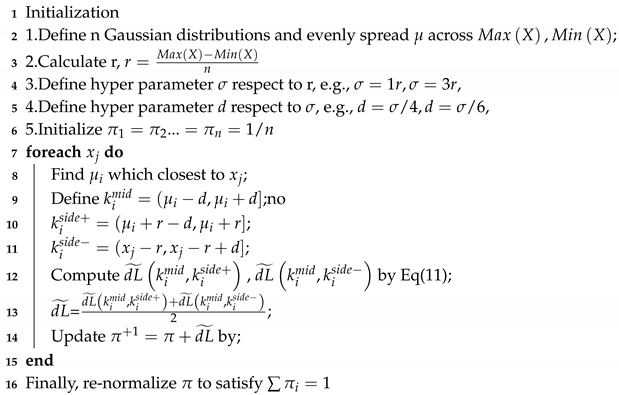Algorithm 2:

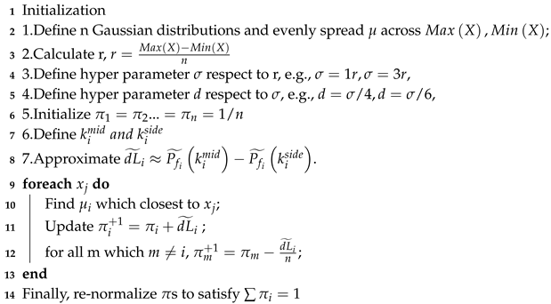3. Numerical Experiments

In this section, we show our algorithm accuracy by approximating arbitrary probability density. 2 neural network applications are shown which implementing GMM into neural network while applying our learning algorithm to learn feasible GMM. Metric for valuating accuracy of density estimation is given by Equation (9). It is a estimation for DIL which shown in Section 2.

\begin{matrix} L = & | P_{t r a g e t} \{x \leq μ_{1} - d\} - P_{g m m} \{x \leq μ_{1} - d\} | \\ + \sum_{i = 1}^{n} | P_{t r a g e t} \{μ_{i} \pm d\} - P_{g m m} \{μ_{i} \pm d\} | \\ + | P_{t r a g e t} \{x > μ_{n} + d\} - P_{g m m} \{x > μ_{n} + d\} | \end{matrix}

(9)

There are a couple of benefits to measuring our estimation accuracy by Equation (9). First, it is simple to calculate. Second, when we do not have the current form of target density, we can still manage to calculate the loss by discrete statistical estimation. Third, it has a clear minimum and maximum, which is [0,2]. The proof is given below:

\begin{matrix} L & \leq | P_{t r a g e t} \{x \leq μ_{1} - d\} - 0 | + \sum_{i = 1}^{n} | P_{t r a g e t} \{μ_{i} \pm d\} - 0 | \\ + | P_{t r a g e t} \{x > μ_{n} + d\} - 0 | + | 0 - P_{g m m} \{x \leq μ_{1} - d\} | \\ + \sum_{i = 1}^{n} | 0 - P_{g m m} \{μ_{i} \pm d\} | + | 0 - P_{g m m} \{x > μ_{n} + d\} | \end{matrix}

That means

0 \leq L \leq 2

3.1. Random Density Approximation

In this subsection, we test the algorithm performance by learning randomly generated mixture distributions. Considering the conditions given by Section 2.4, mixture distributions with smooth shapes are best for GMM to work with generally. In order to further investigate model efficacy, we also test our model with distributions that mix with non-smooth distributions, which, in our case, uniform distributions are used to build these target mixture distributions. Two random generated cases are illustrated with Figure 3, Figure 4 and Figure 5 to show the learning process. The upper subplot in Figure 3. is target distribution 1, which is mixed by 8 normal distributions. The lower subplot in Figure 3. is target distribution 2, which mixes with normal distributions, T distributions as well as uniform distributions. Figure 4 shows our initial GMM before learning. Figure 5 and Figure 6 show the comparison of target density and learned GMM. GMM with 200 components is applied to learn the target distribution. We sample 5000 data points from each target distribution as training dataset.

The target distribution 1 refers to those situations where GMM can perform best. Geometrically speaking, while target distributions are mixed with components which share a bell shape like structure, using GMM to approximate is an appropriate choice instinctively. But in situations like target distribution 2, while we add uniform distribution in the component distribution set, it becomes difficult for GMM to work with unless we have more components. In Figure 4, it tells the story straight away. We can see that the density of our initial GMM before training is very close to a uniform distribution. More components allow GMM to learn more structure. For example, straight lines and deep cuts. This implies that if we want to approximate arbitrary densities which are not limited by multimodal, flat peaks, deep cuts and all possible variations, we need higher order mixture components for our GMM. In the classic EM algorithm, considering we have 200 normal components, parameters that we need to learn for a GMM are

3 \times 200

. There are handful amount of learning to be done. As we proposed in this paper, by fixing

μ

and

σ

as bases and smoothness, the remaining parameters needed to be learned are limited down to 200.

Figure 5 and Figure 6 show that the proposed algorithm works well to approximate target density. Comparing the two results, target density 1, which mixes with bell shape like distributions, works better than target distribution 2, which mixes with uniform distributions and others. But over all, even though the result in Figure 6 does have many unwanted sags and crests, GMM approximation still manages to capture those key features of target density. In Figure 5 and Figure 6, it shows the performance of two different algorithms mentioned in Section 2.5. There are three curves shown in the graph. Green is the target density, the blue curve is the density of learned GMM by algorithm 2 and the orange curve is the density of learned GMM by Algorithm 1. The blue curve and orange curve almost overlap each other. The difference between algorithms is almost unnoticeable.

Table 1 and Table 2 present average losses(L) in Equation 9 over 20 experiments. In Table 1, the target distribution is randomly generated Gaussian mixture distributions. Some approximation examples are shown in Figure 7 subplots (1)-(3). Table 2 presents the average L by approximating the mixture distribution of which components contain Normal, T and Uniform distributions. Some examples are shown in Figure 7 subplots (4)-(6). Tables show that using GMM approximating target distributions with normal components is generally better than target distributions mixed with distributions containing various types. They also reveal an interesting finding that adjusting

σ

will change the overall accuracy. For target distributions mixed with normal distributions, the increase

σ

from 1*r to 3*r gives a better outcome. But when the target density gets more complex, a sigma with 2*r works the best. Comparing with subplots 1-3 and subplots 4-6 in Figure 7, distributions with extreme features require a

σ

that is not too large and too small. The smaller the

σ

goes, it results in higher expressiveness but less smooth overall. Surprisingly, from what we have discussed in section 2.4, the proposed learning algorithm works best for continuous smooth density, but our experiments show that our proposed method still manages to capture all major character of target distributions and produce relatively good approximations. Table 1 and Table 2 implies that when we make predictions, the errors of probability are lower than 0.095. Since the metric function L has a clear upper and lower bound which is

0 \leq L \leq 2

. That means that errors in our experiments are less than

5 %

The number of mixture components and data size should have a certain relationship that affects the overall model performance. We have not yet found a proper solution to this matter, but we have carried out experiments to demonstrate the relationship between how data size affects the accuracy under different amount of mixed components.

In Table 3, we run 30 experiments for each GMM with components sized from 10 to 1000. We apply algorithm 2 with

σ = 3 * r

for the learning process. Target distributions are randomly generated mixture distributions the same as experiments in Table 1 and Table 2. Compared with experiments carried out in Table 1, it shows that with components less than 200, an increase in the data size does not increase performance. With GMM constructed of 100 components, information loss L at data size 20000 and 50000 are 0.0778 and 0.065 is worse than GMM with 200 components learning under 5000 data points. By increasing data size, components with 200 components’ performance continuously improve from 0.04447 down to 0.025. Under the same data size, increasing the size of components does not necessarily lead to a better outcome after a certain level. In data size 20000, components sizes 500 and 1000 do not perform better than 200. But in data size 50000, GMM with 500 components outperforms the rest of any other GMMs. These discoveries match our idea of GMM distribution decomposition intuitively. If we want to decompose a distribution, a certain number of components are needed to achieve an appropriate level of detail representation of a density. In order to learn finer details, more data points and more components are needed. In our experiment, 200 components showed enough robustness for practical usage. It managed to increase accuracy from data size 5000 up to 50000.

3.2. Neural Network Application

In this section, we present a couple of neural network applications with GMMs and our GMMs learning algorithms. The first one is handwritten digits generation using Autoencoder, where GMM is used to learn encoder output distribution. The second one is style transfer, where GMM is used to learn gram matrix distribution.

3.2.1. Mnist Data Set of Handwritten Digits Generation

In this experiment, we carry out the same numerical experiment as [11]. In Kolouri et al experiment, they demonstrated how to learn an embedding layer(latent variables) by GMM using Sliced Wasserstein Distance. In our approach, we learn the GMM by proposed algorithms. The neural network model structure is exactly the same as [11] proposed. which is a generative adversarial network constructed by pairing a Autoencoder generator and a simple convolution neural network with classification output as discriminator. [24,25,26,27,28]. The whole process is illustrated in Figure 8.

In Figure 9, we show our results as well as compare them with the learning method proposed at [11]. On the left-hand side of Figure 9, we have our results that are randomly sampled from our learned GMM distributions. Compare with [11], our result at the number 8 is more clear than SW-GMM and EM-GMM. Also, at number 9, our generation are less confused with number 4. At number 7, our result shows more variety. Our learning method captures different types of digit 7. Some rounder shapes and dash in the middle are also captured in our learned GMM. Most of the random samples in our results do not contain a large number of unrecognizable generations, such as results generated by EM-GMM and SW-GMM highlighted in red in Figure 9.

It is worth mentioning that, in our training process, in order to gain faster convergence, we slightly amended the loss function of GAN. The loss function for GAN is Equation (10).

J^{(G)} = - α \frac{1}{2} E_{z} l o g (1 - D (G (z))) + {‖ x - G (z) ‖}^{2}

(10)

where

J^{(G)}

is the loss of a generator.

α

is a constant to adjust the level of discriminator loss.

\frac{1}{2} E_{z} l o g (1 - D (G (z)))

is the discriminator loss same as [29]. x is the target image and

G (z)

is output image generated by generator.

Following up the notation given on [29], for the generator loss, we multiply

α

to the cross-entropy loss to regulate how much we want to listen to the discriminator. Adding in Mean Square Loss guides the generator to generate images close to the dataset.

Another interesting experiment is that we performed random mixing of a couple of GMM samples through different classes. There are 4 examples shown in Figure 10. Despite the fact that those generated images are becoming intractable as a number, our generated images still manage to maintain features from input categories. For example, 0 and 4 generated an image similar to 9. The example in top right is the image generated by GMM samples randomly combined from class 0 and 3. Compared with the normalization flow model, through an auto regressive process, it manages to diversify the latent space into a more accurate one-to one mapping to the data set [30]. In the diffusion model, it uses stochastic processes to add in noise and achieve precise mapping of the data. Adding noise to the image diverts two similar images that create a one-to-one-path way for the neural network to work with [31,32]. In our work, simply applying GMM as an intermediate for latent variables achieves similar effect. Variables for each class are well segmented and that allows us to create random combinations of features. It is easy to use and capable of having more control over generated images, as Figure 10 is shown. It could be potentially useful for language to image models by mapping words as a GMM distribution. Because values of latent variables are randomly sampled, generated images won’t easily fall into repetitive.

3.2.2. Style Transfer

Here we introduce a modified version of style transfer [23] algorithm which turns gram matrix into GMM. Gram matrix is the core of the style transfer. It represents the level of correlation between each extracted feature which is calculated by a trained neural network. In our experiments, we followed the original work and apply trained VGG19 [33] for feature extraction. One of the reasons why introducing GMM into the algorithm is because of variation. A certain gram matrix means a certain outcome for the algorithm. We could achieve changing learning rate or the weight between style features and content features to add variation to the algorithm, but sometimes changing those parameters aggressively will lead to a chaotic outcome. Additionally, when we try mixing a couple of styles at the same time, the classic method can hardly control the level of feature mixing between two styles. One way to tackle these problems is turning a gram matrix into a distribution to perform random sampling. A random sample of gram matrix randomizes the feature combination. It is similar to what we show in the MNIST handwritten digits generation experiments where mixing features stochastically can create new digits.

Figure 11 shows the process of how a gram matrix is produced. Passing an image into VGG19 produces output features from each layer. Take 5 output features from each block and perform Equation (14) to calculate the gram matrix. For convenience, we call it VGG19 feature extraction module.

G_{i j}^{l} = \sum_{k} F_{i k}^{l} F_{j k}^{l},

(11)

In Figure 12, we illustrate how to prepare a gram matrix data set as well as the whole procedure of the algorithm. First, we randomly crop two style images, pass them separately into the VGG19 feature extraction module which gives us a data set of gram matrix for each layer. Second, we learn GMM from a gram matrix dataset for each layer by Algorithm 2. Third, sample the gram matrix and apply the same optimisation step as [23]. Dataset determine the probability of features in the gram matrix. For example, if we randomly crop 25 images from style 1 and 75 images from style 2, the gram matrix dataset contains 1/4 data points from style 1 and 3/4 from style 2. While we sample the gram matrix distributions, the sampled gram matrix is likely to contain

25 %

values from style 1 and

75 %

values from style 2. Figure 13 shows a graphical example of our approach. We use two famous Vincent Van Gogh paintings. ’The Starry Night’ as target image as well as style image and ’Sunflowers’ as style image 2. While we gradually increase the size of style 2 images in the data set, the output image shows more and more features from style image 2. By learning different random sampled gram matrices, we notice that each output image shares the same style but features are noticeably different from one to another. Almost like changing position and angle of each stroke. Combining all output images together will create an effect like features are flowing in the painting. Here is a

y o u t u b e

https://youtu.be/yP22_ycAqMA video showcase the results. Feature mixing level between two style are

0 %

10 %

20 %

...

80 %

as Figure 13 shows. 10 images are produced at a time from each mixing level. This approach lets us explore what features neural networks are capable of extracting and how they affect the final outcome.

4. Conclusions and Future Work

In this work, by taking the idea of Fourier decomposition, we show that GMMs with large-sized components are capable of approximating arbitrary distributions. 2 simple easy-to-use algorithms are introduced to learn GMMs. Several numerical experiments are carried out to show the effectiveness of our algorithm. We also demonstrated how to apply GMMs to natural networks. Our algorithm learns latent space for Autoencoder handwritten digits generation and gram matrix for style transfer. By randomly mixing the sampled latent variables across different categories, the neural network is able to generate meaningful images combining features from different categories. In the same fashion as how we deal with latent variables in the Autoencoder, we apply GMM in style transfer gram matrix. This allows us to add variation and uncertainty to the algorithm, which opens up more options for us to manipulate neural networks as well as explore feature combinations in neural networks.

In the future, we will work on more precise theoretical proof of the argument of whether arbitrary distributions can be precisely decomposed by GMM. Since our experiment shows that GMM allows us to gain more control and variation on neural networks, we will look further to build more sophisticated applications.

References

Murphy, K.P. Machine learning: A probabilistic perspective (adaptive computation and machine learning series), 2018.
Gal, Y. What my deep model doesn’t know. Personal blog post 2015. [Google Scholar]
Kendall, A.; Gal, Y. What uncertainties do we need in bayesian deep learning for computer vision? Advances in neural information processing systems 2017, 30. [Google Scholar]
Der Kiureghian, A.; Ditlevsen, O. Aleatory or epistemic? Does it matter? Structural safety 2009, 31, 105–112. [Google Scholar] [CrossRef]
McLachlan, G.J.; Rathnayake, S. On the number of components in a Gaussian mixture model. Wiley Interdisciplinary Reviews: Data Mining and Knowledge Discovery 2014, 4, 341–355. [Google Scholar] [CrossRef]
Li, J.; Barron, A. Mixture density estimation. Advances in neural information processing systems 1999, 12. [Google Scholar]
Genovese, C.R.; Wasserman, L. Rates of convergence for the Gaussian mixture sieve. The Annals of Statistics 2000, 28, 1105–1127. [Google Scholar] [CrossRef]
Dempster, A.P.; Laird, N.M.; Rubin, D.B. Maximum likelihood from incomplete data via the EM algorithm. Journal of the Royal Statistical Society: Series B (Methodological) 1977, 39, 1–22. [Google Scholar] [CrossRef]
Verbeek, J.J.; Vlassis, N.; Kröse, B. Efficient greedy learning of Gaussian mixture models. Neural computation 2003, 15, 469–485. [Google Scholar] [CrossRef]
Du, J.; Hu, Y.; Jiang, H. Boosted mixture learning of Gaussian mixture hidden Markov models based on maximum likelihood for speech recognition. IEEE transactions on audio, speech, and language processing 2011, 19, 2091–2100. [Google Scholar] [CrossRef]
Kolouri, S.; Rohde, G.K.; Hoffmann, H. Sliced wasserstein distance for learning gaussian mixture models. Proceedings of the IEEE Conference on Computer Vision and Pattern Recognition, 2018, pp. 3427–3436.
Srebro, N. Are there local maxima in the infinite-sample likelihood of Gaussian mixture estimation? International Conference on Computational Learning Theory. Springer, 2007, pp. 628–629.
Améndola, C.; Drton, M.; Sturmfels, B. Maximum likelihood estimates for gaussian mixtures are transcendental. International Conference on Mathematical Aspects of Computer and Information Sciences. Springer, 2015, pp. 579–590.
Jin, C.; Zhang, Y.; Balakrishnan, S.; Wainwright, M.J.; Jordan, M.I. Local maxima in the likelihood of gaussian mixture models: Structural results and algorithmic consequences. Advances in neural information processing systems 2016, 29. [Google Scholar]
Chen, Y.; Georgiou, T.T.; Tannenbaum, A. Optimal transport for Gaussian mixture models. IEEE Access 2018, 7, 6269–6278. [Google Scholar] [CrossRef] [PubMed]
Li, P.; Wang, Q.; Zhang, L. A novel earth mover’s distance methodology for image matching with gaussian mixture models. Proceedings of the IEEE International Conference on Computer Vision, 2013, pp. 1689–1696.
Beecks, C.; Ivanescu, A.M.; Kirchhoff, S.; Seidl, T. Modeling image similarity by gaussian mixture models and the signature quadratic form distance. 2011 International Conference on Computer Vision. IEEE, 2011, pp. 1754–1761.
Jian, B.; Vemuri, B.C. Robust point set registration using gaussian mixture models. IEEE transactions on pattern analysis and machine intelligence 2010, 33, 1633–1645. [Google Scholar] [CrossRef] [PubMed]
Yu, G.; Sapiro, G.; Mallat, S. Solving inverse problems with piecewise linear estimators: From Gaussian mixture models to structured sparsity. IEEE Transactions on Image Processing 2011, 21, 2481–2499. [Google Scholar] [PubMed]
Campbell, W.M.; Sturim, D.E.; Reynolds, D.A. Support vector machines using GMM supervectors for speaker verification. IEEE signal processing letters 2006, 13, 308–311. [Google Scholar] [CrossRef]
Ballard, D.H. Modular learning in neural networks. Aaai, 1987, Vol. 647, pp. 279–284.
LeCun, Y. PhD thesis: Modeles connexionnistes de l’apprentissage (connectionist learning models); Universite P. et M. Curie (Paris 6), 1987.
Gatys, L.A.; Ecker, A.S.; Bethge, M. A neural algorithm of artistic style. arXiv preprint arXiv:1508.06576 2015.
Hinton, G.E.; Zemel, R. Autoencoders, minimum description length and Helmholtz free energy. Advances in neural information processing systems 1993, 6. [Google Scholar]
Schwenk, H.; Bengio, Y. Training methods for adaptive boosting of neural networks. Advances in neural information processing systems 1997, 10. [Google Scholar]
LeCun, Y. The MNIST database of handwritten digits. http://yann. lecun. com/exdb/mnist/ 1998.
Goodfellow, I.; Pouget-Abadie, J.; Mirza, M.; Xu, B.; Warde-Farley, D.; Ozair, S.; Courville, A.; Bengio, Y. Generative adversarial networks. Communications of the ACM 2020, 63, 139–144. [Google Scholar] [CrossRef]
Li, J.; Monroe, W.; Shi, T.; Jean, S.; Ritter, A.; Jurafsky, D. Adversarial learning for neural dialogue generation. arXiv preprint arXiv:1701.06547 2017.
Goodfellow, I. Nips 2016 tutorial: Generative adversarial networks. arXiv preprint arXiv:1701.00160 2016.
Kingma, D.P.; Salimans, T.; Jozefowicz, R.; Chen, X.; Sutskever, I.; Welling, M. Improved variational inference with inverse autoregressive flow. Advances in neural information processing systems 2016, 29. [Google Scholar]
Ho, J.; Jain, A.; Abbeel, P. Denoising diffusion probabilistic models. Advances in Neural Information Processing Systems 2020, 33, 6840–6851. [Google Scholar]
Song, Y.; Ermon, S. Generative modeling by estimating gradients of the data distribution. Advances in Neural Information Processing Systems 2019, 32. [Google Scholar]
Simonyan, K.; Zisserman, A. Very deep convolutional networks for large-scale image recognition. arXiv preprint arXiv:1409.1556 2014.

Figure 1. Example of fitted GMM and target density in region

ω_{i}

Figure 1. Example of fitted GMM and target density in region

ω_{i}

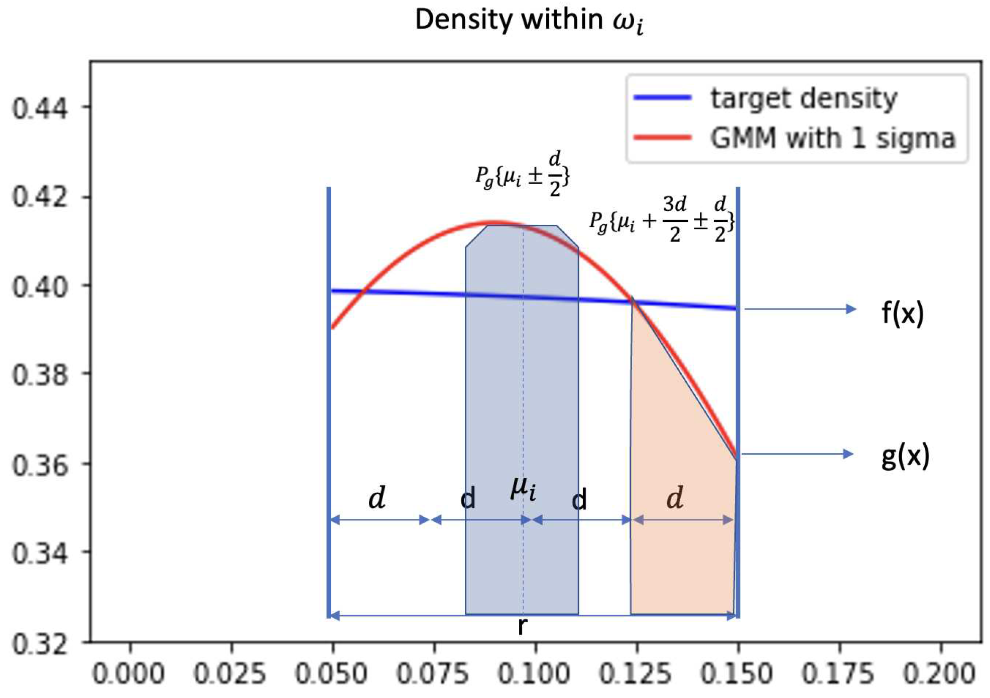
Figure 2. Example of GMM and target density in region

ω_{i}

with larger

σ

Figure 2. Example of GMM and target density in region

ω_{i}

with larger

σ

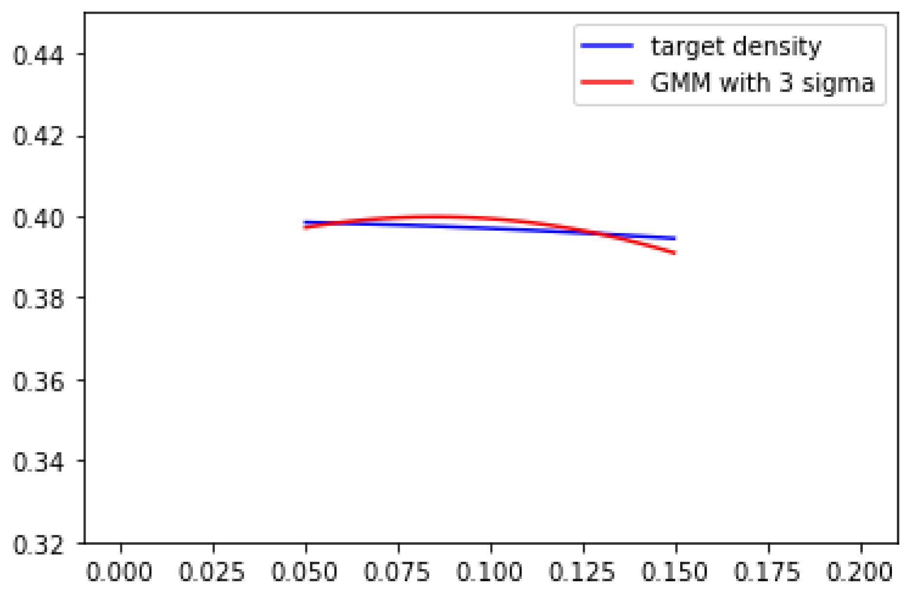
Figure 3. Target Distributions

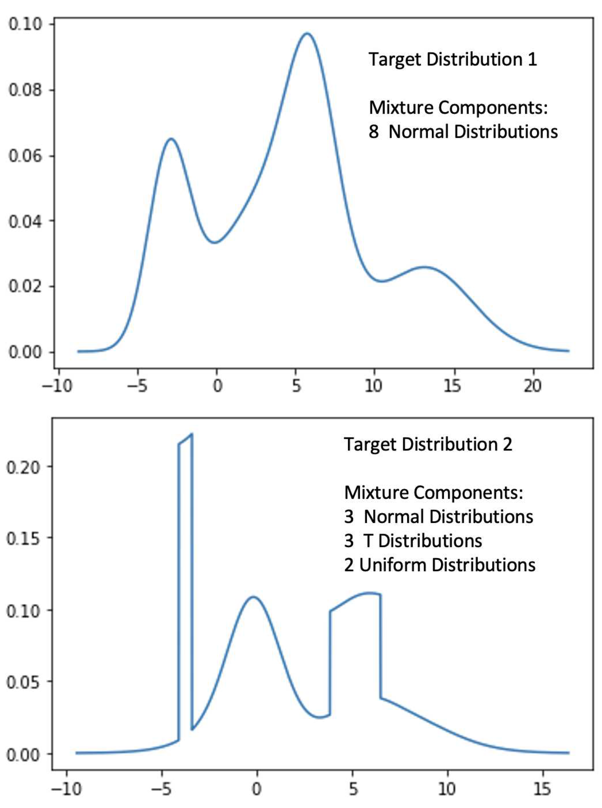
Figure 4. Initialize GMM

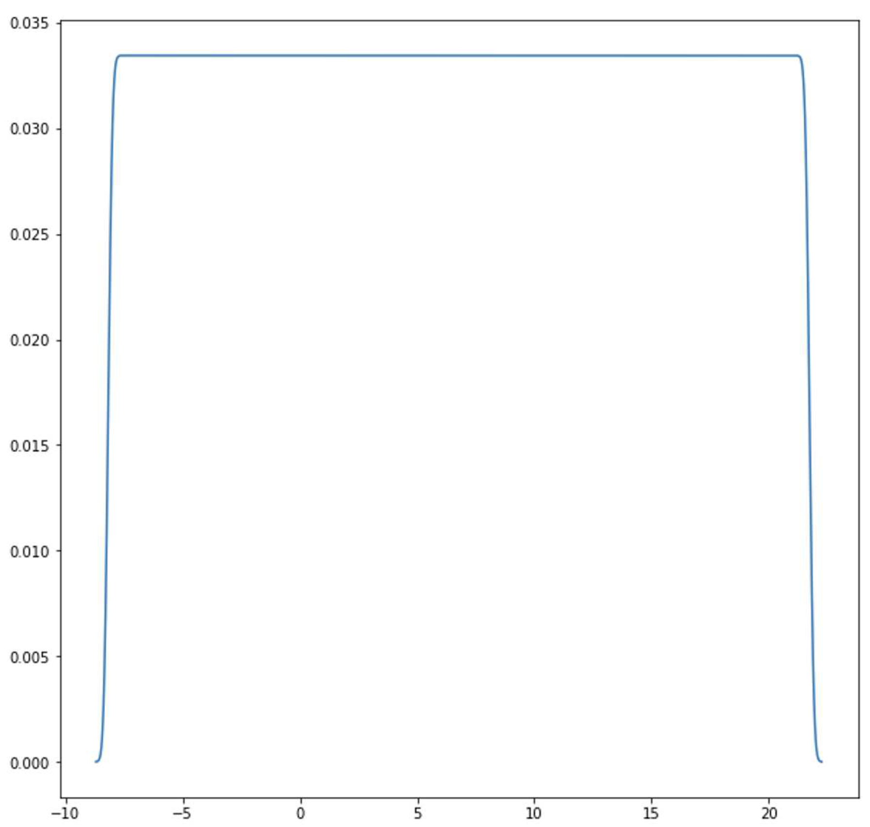
Figure 5. Trained GMM vs Target Distribution 1

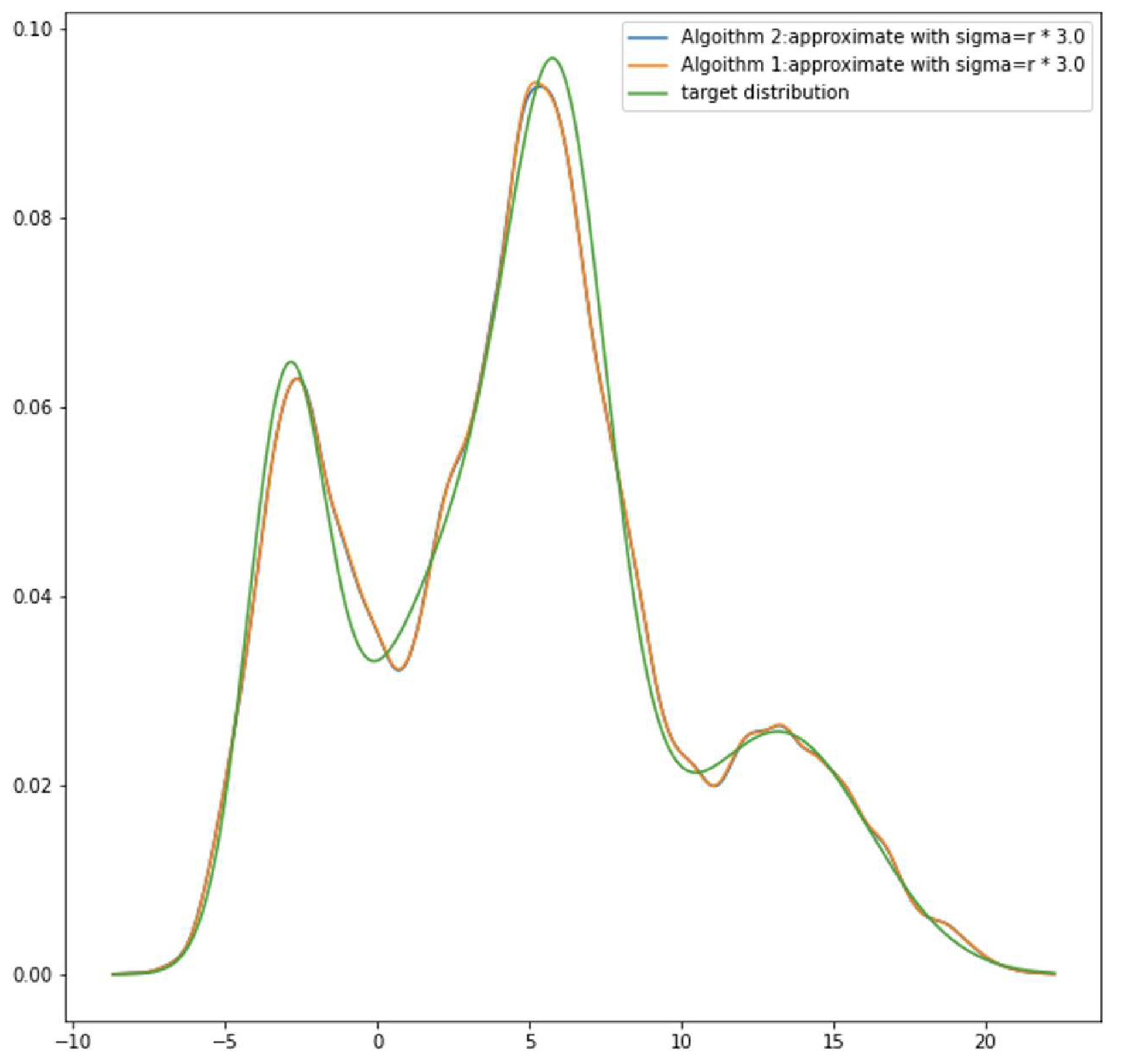
Figure 6. Trained GMM vs Target Distribution 2

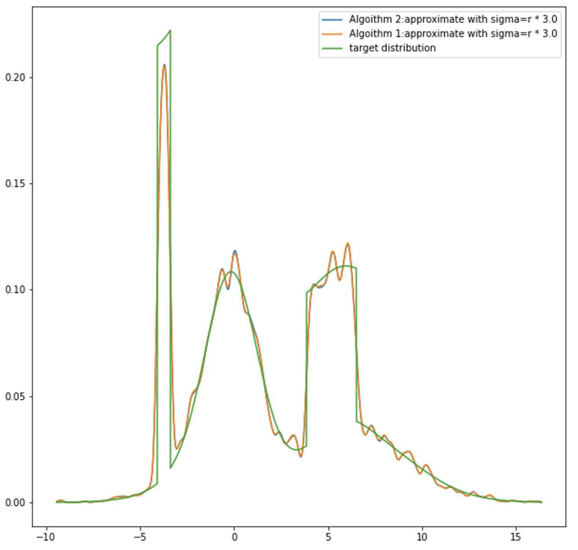
Figure 7. Other trained examples

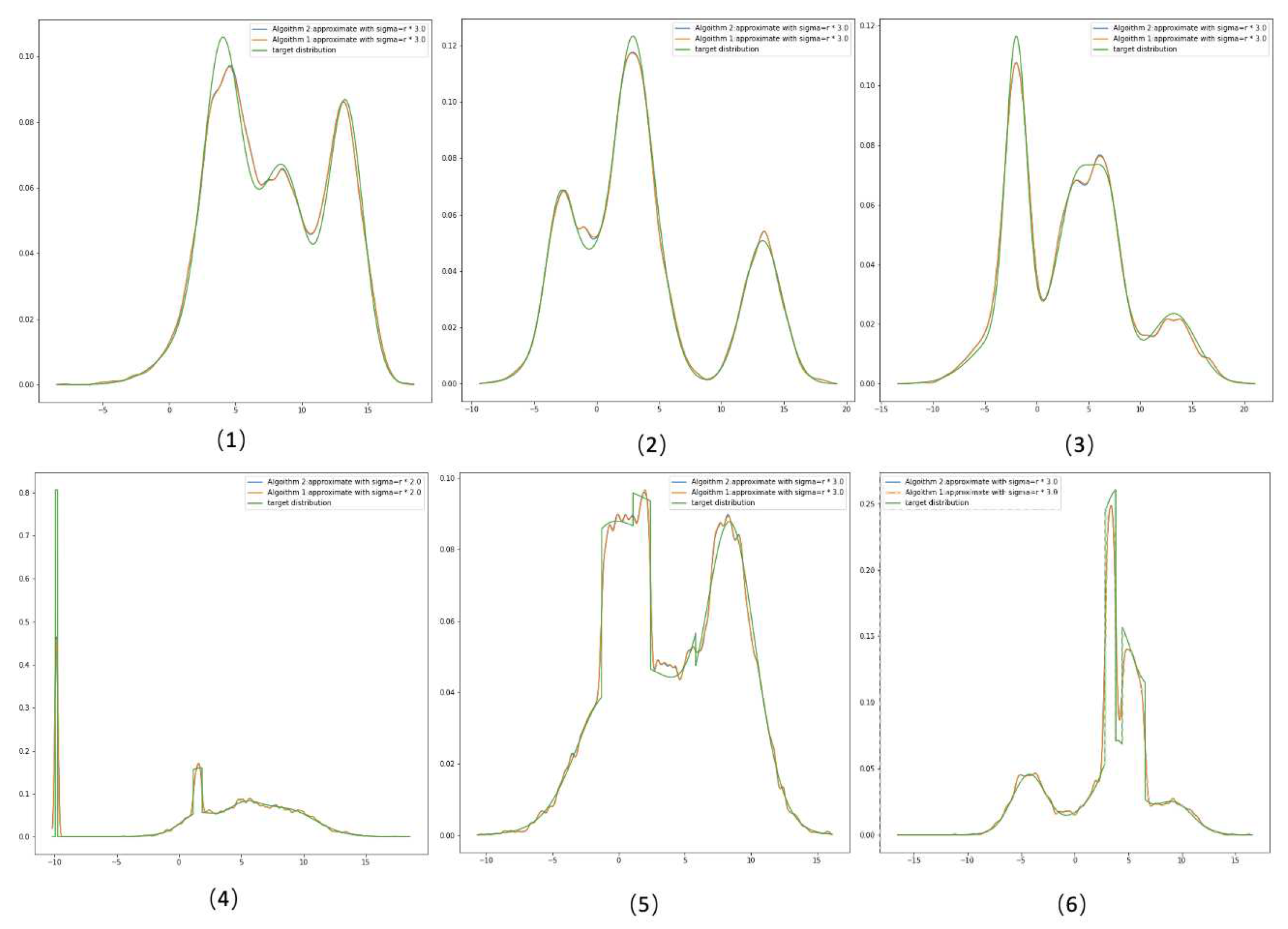
Figure 8. Model Structure

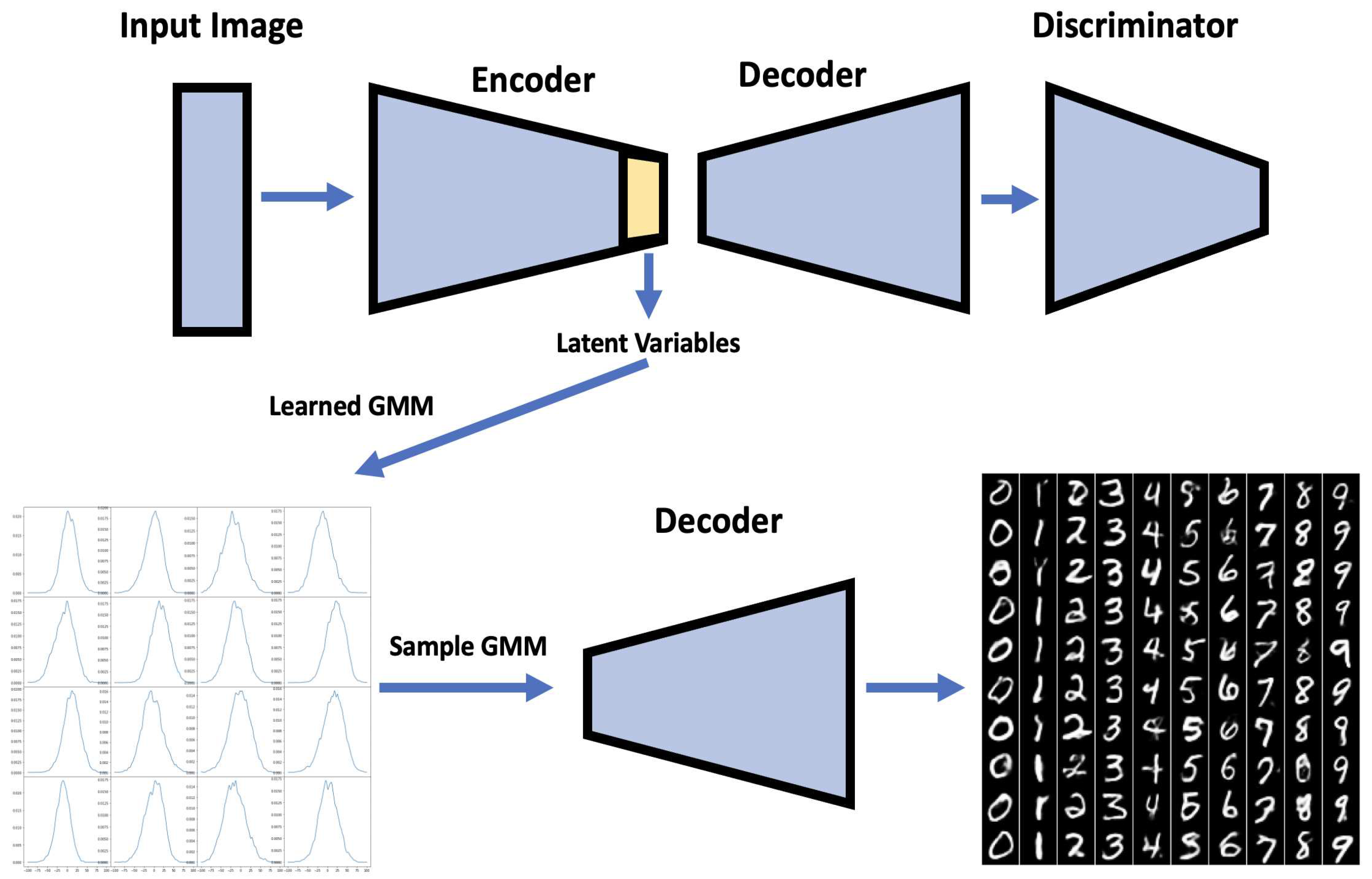
Figure 9. Result comparison

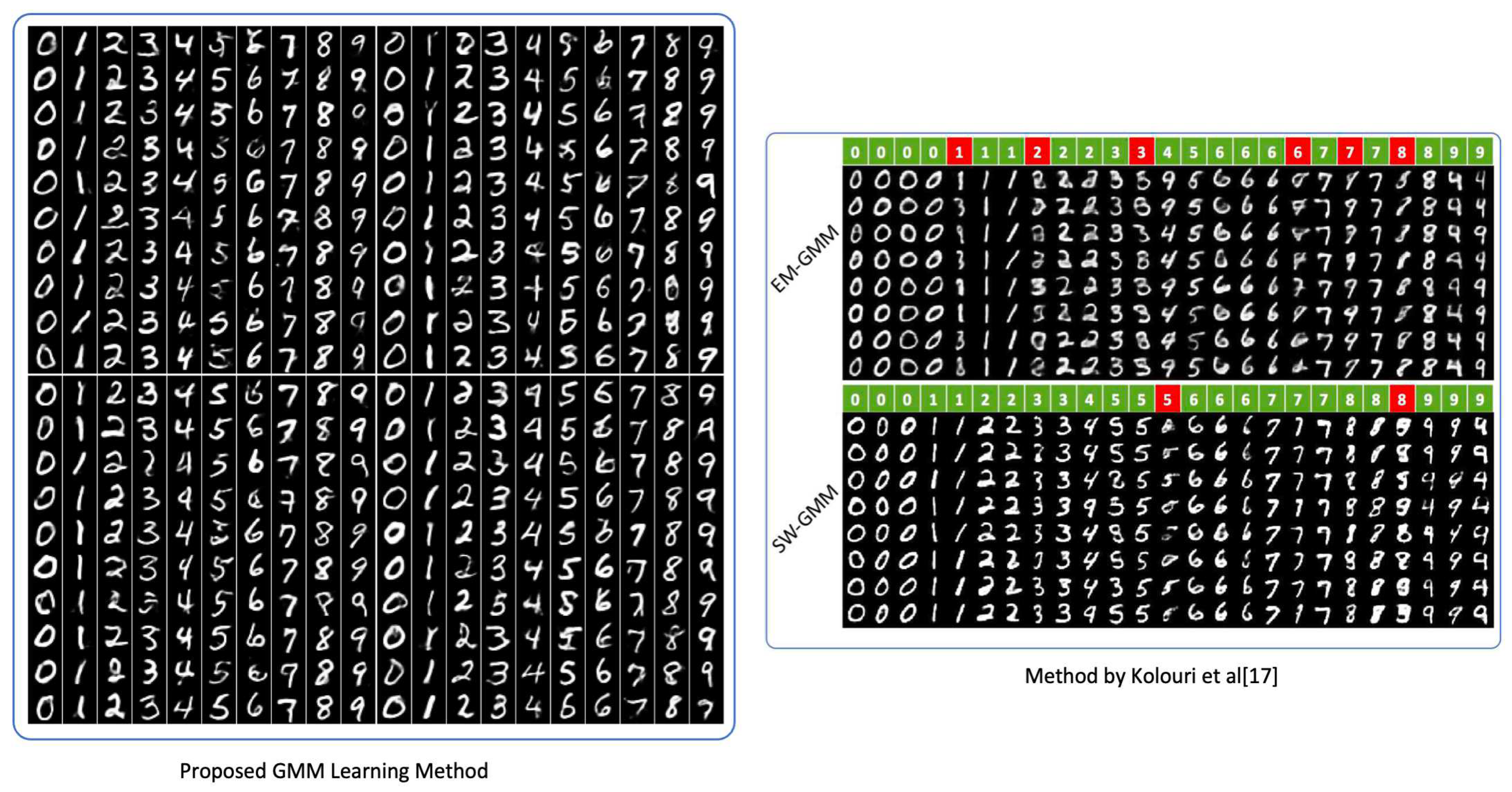
Figure 10. Random Mixing

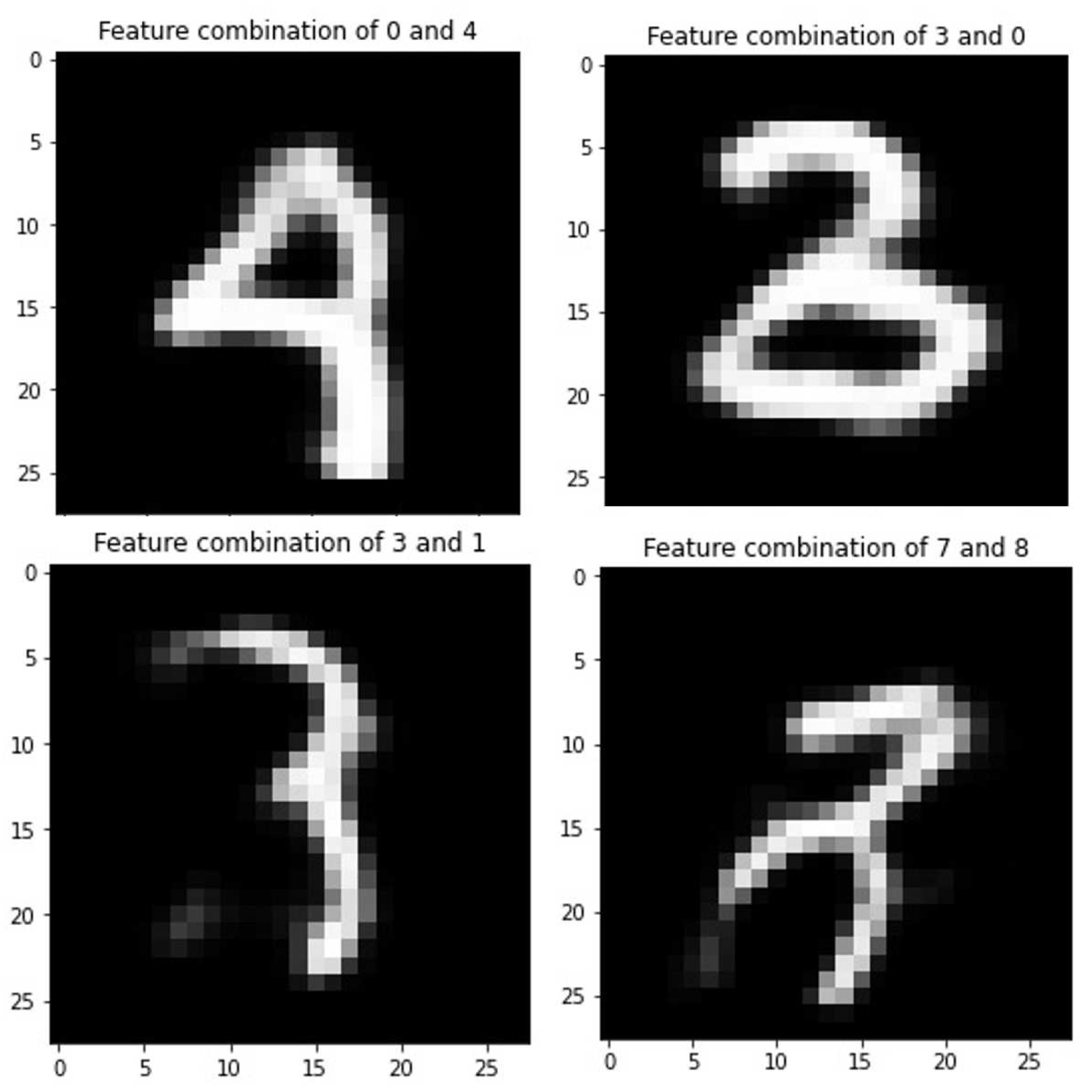
Figure 11. Result comparison

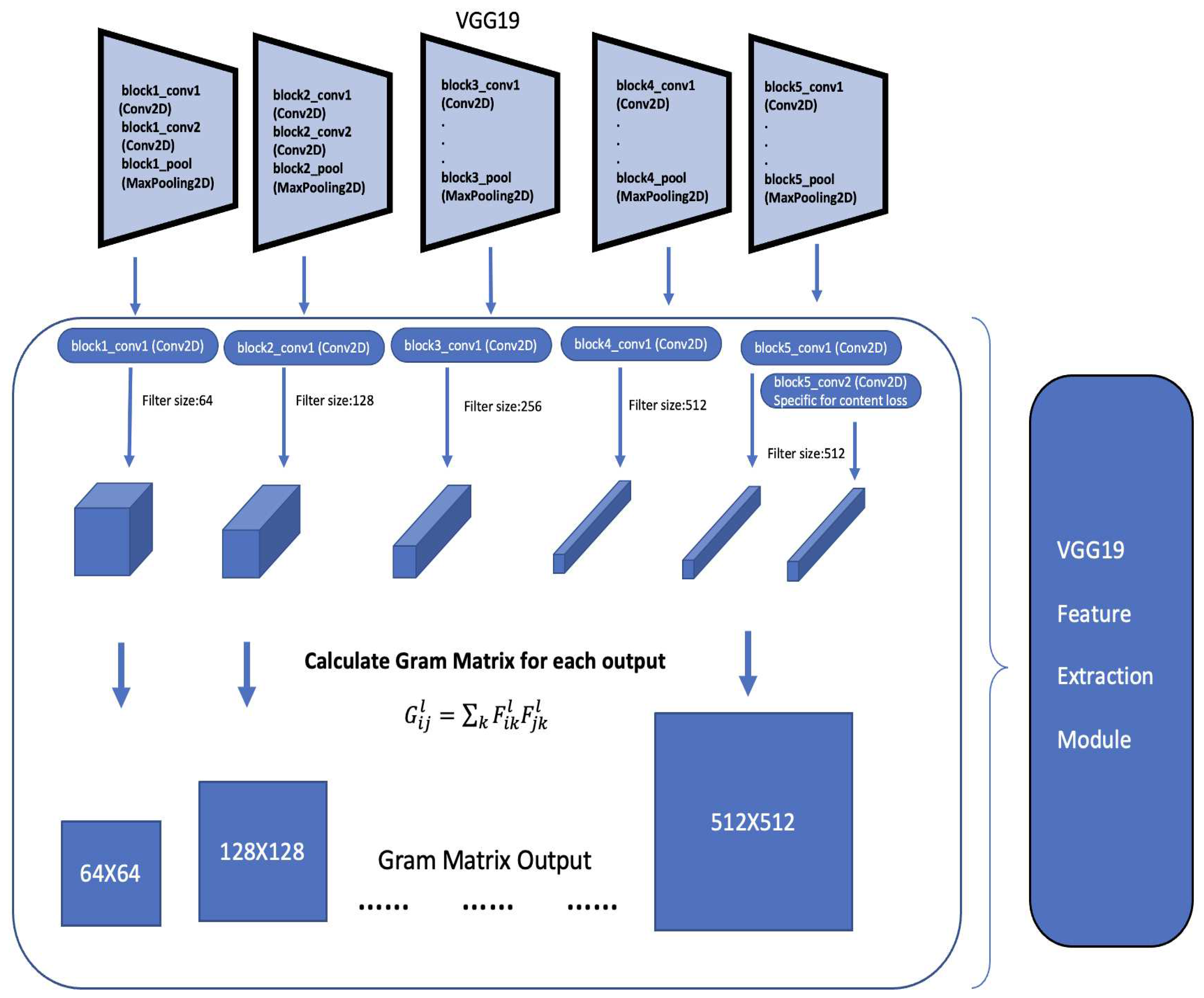
Figure 12. Result comparison

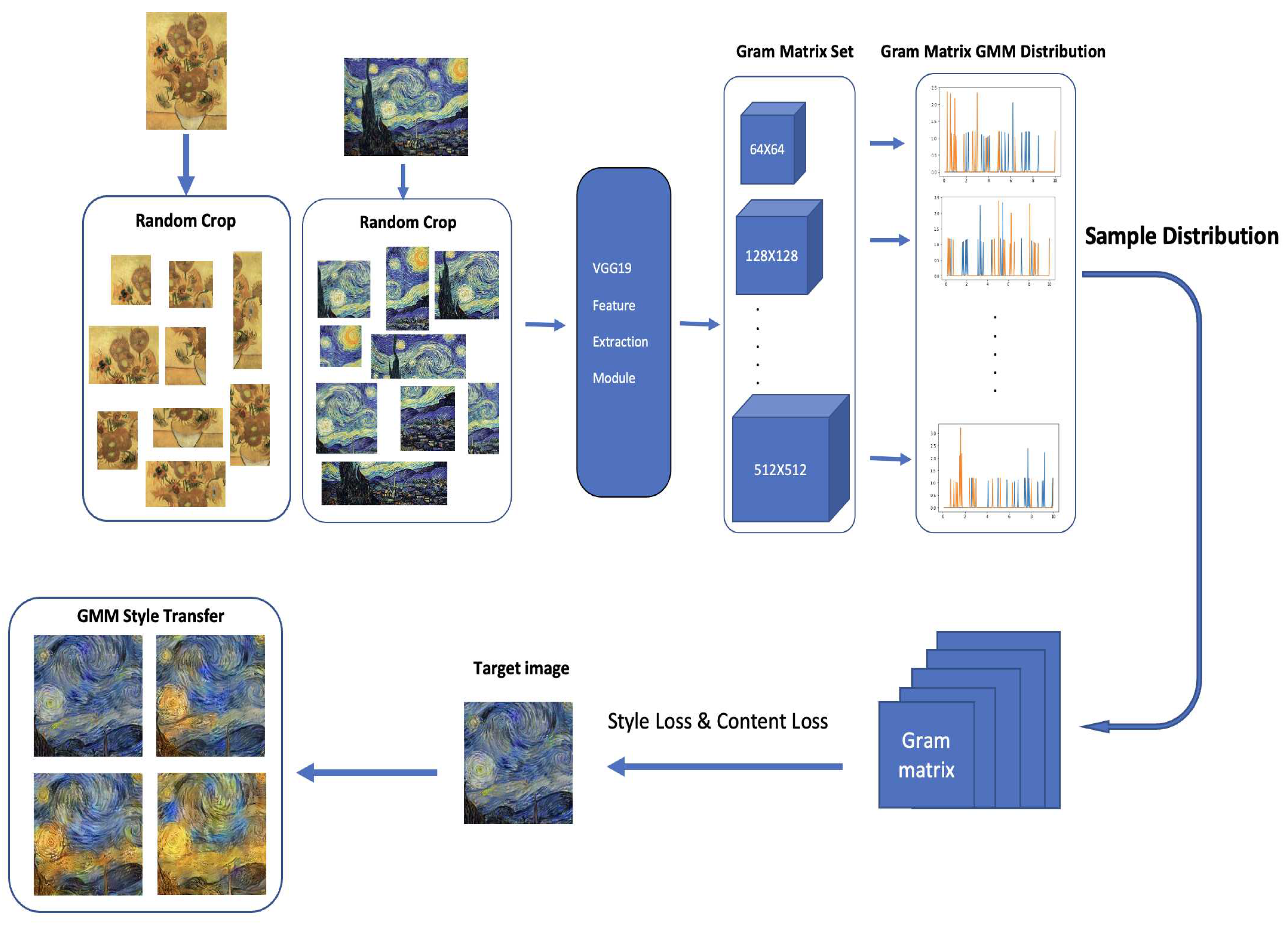
Figure 13. Random Mixing

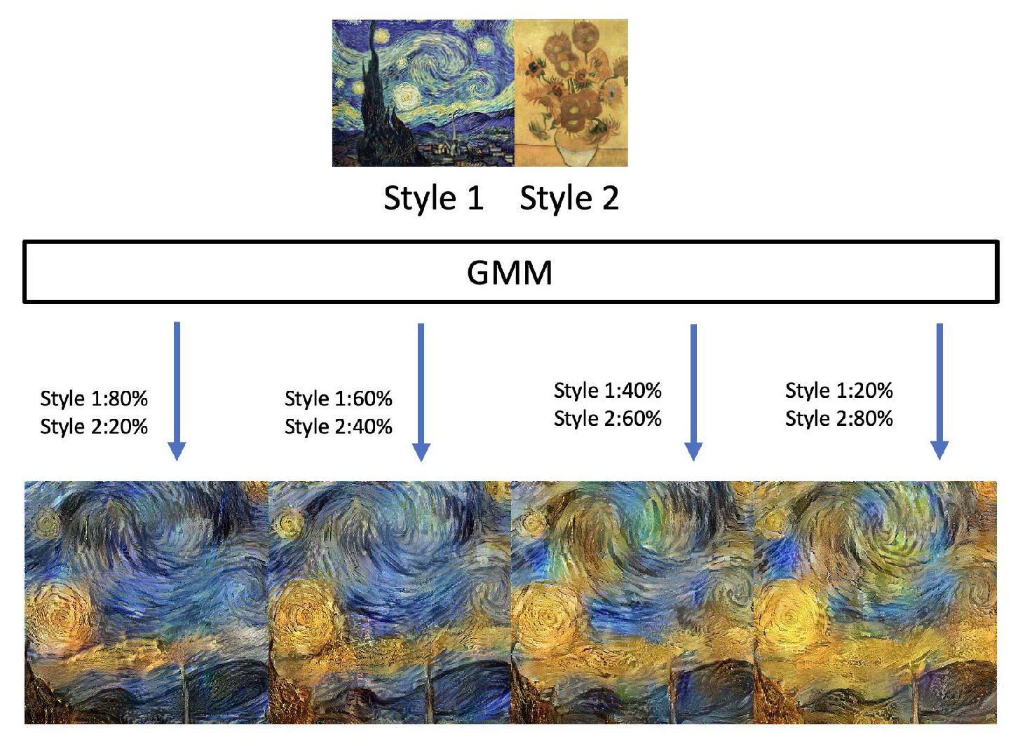
Table 1. Average Loss of 20 Experiments With 8 random Gaussian Components. Data size: 5000 data points

Average Loss of 20 Experiments
Algorithm 1
$σ = 1 * r$	$σ = 2 * r$	$σ = 3 * r$
$L =$ 0.07099	$L =$ 0.05091	$L =$ 0.044296
Algorithm 2
$σ = 1 * r$	$σ = 2 * r$	$σ = 3 * r$
$L =$ 0.06866	$L =$ 0.05085	$L =$ 0.04447

Table 2. Average Loss of 20 Experiments With 8 Non-Gaussian random Components. Data size: 5000 data points

Average Loss of 20 Experiments
Algorithm 1
$σ = 1 * r$	$σ = 2 * r$	$σ = 3 * r$
$L =$ 0.08912	$L =$ 0.08738	$L =$ 0.09432
Algorithm 2
$σ = 1 * r$	$σ = 2 * r$	$σ = 3 * r$
$L =$ 0.08678	$L =$ 0.08749	$L =$ 0.09446

Table 3. Average Loss of 25 Experiments With different numbers of components compare with data size 20000 data points and 50000 data points.

Average Loss of 30 Experiments with Data size 20000
Numbers of Components
10	30	50	100	200	500	1000
$L = 0.710$	$L = 0.336$	$L = 0.200$	$L = 0.0778$	$L = 0.0295$	$L = 0.0326$	$L = 0.0378$
Average Loss of 30 Experiments with Data size 50000
Numbers of Components
10	30	50	100	200	500	1000
$L = 0.715$	$L = 0.364$	$L = 0.210$	$L = 0.065$	$L = 0.025$	$L = 0.0203$	$L = 0.0289$

Disclaimer/Publisher’s Note: The statements, opinions and data contained in all publications are solely those of the individual author(s) and contributor(s) and not of MDPI and/or the editor(s). MDPI and/or the editor(s) disclaim responsibility for any injury to people or property resulting from any ideas, methods, instructions or products referred to in the content.

© 2023 by the authors. Licensee MDPI, Basel, Switzerland. This article is an open access article distributed under the terms and conditions of the Creative Commons Attribution (CC BY) license (http://creativecommons.org/licenses/by/4.0/).

Copyright: This open access article is published under a Creative Commons CC BY 4.0 license, which permit the free download, distribution, and reuse, provided that the author and preprint are cited in any reuse.

Downloads

497

Views

211

Comments

Subscription

Notify me about updates to this article or when a peer-reviewed version is published.

MDPI Initiatives

Important Links

Choose an area of interest and we will send you notifications of new preprints at your preferred frequency.

Disclaimer

An Efficient Gaussian Mixture Model and It's Application to Neural Network

Abstract

Keywords:

Subject:

1. Introduction

2. Decompose Arbitrary Density by GMM

2.1. General Concept of GMM Decomposition

2.2. Approximate Arbitrary Density by GMM

2.3. Density Information Loss

2.4. Learning Algorithm

3. Numerical Experiments

3.1. Random Density Approximation

3.2. Neural Network Application

3.2.1. Mnist Data Set of Handwritten Digits Generation

3.2.2. Style Transfer

4. Conclusions and Future Work

References

MDPI Initiatives

Important Links

Subscribe