
Submitted:
08 February 2023
Posted:
08 February 2023
You are already at the latest version
Abstract
Coastal marine ecosystems worldwide, like Florida Bay, are increasingly affected by tide alteration and anthropogenic disturbances which affect water quality imbalance leading to algal blooms. Increased bloom persistence is a serious threat due to the long-lasting impact on processes like carbon cycle and services like species presence. However, exploring eco-environmental feedback patterns of algal blooms remains challenging and poorly investigated, also due to the paucity of data.
Florida Bay, taken as an epitome, has long experienced algal blooms in its central and western regions, and in 2006 an unprecedented bloom occurred in the eastern habitats. We analyzed the occurrence of blooms from three perspectives: (1) the spatial spreading networks of chlorophyll-a (CHLa) that pinpoints source and unbalanced habitats; (2) the fluctuations of water quality factors pre- and post-bloom outbreaks to in assess environmental impacts of ecological dysbiosis and target prevention and control of algal of blooms; and (3) the biogeochemical-spreading network topological co-evolution to quantify ecosystemic stability and ecological shift likelihood in long-term.
Here, we propose Transfer Entropy (TE) to quantify dynamical interactions between spatial areas and biogeochemical factors (ecosystem connectome) underpinning bloom emergence and spreading, as well as environmental effects; the Pareto principle is defined for identifying the salient eco-environmental interactions of CHLa. We quantified the spatial dynamics of algal blooms, and thus obtained areas in need for ecological monitoring and potential bloom control. Results show that algal blooms are increasingly persistent over space with long-term negative effects on water quality factor. A dichotomy is reported between spatial ecological corridors of spreading and biogeochemical networks as well as divergence from the optimal eco-organization: randomization of the former due to nutrients' overload and temperature increase leads to scale-free CHLa spreading and extreme outbreaks a posteriori. Subsequently this increases bloom persistence, turbidity and salinity with potentially strong ecological effects on highly biodiverse and vulnerable areas such as tidal flats and marshes.
Algal blooms are important ecosystem regulators of nutrient cycles; however, beyond limit chlorophyll-a outbreaks cause aquatic species mortality due to their effect on water turbidity, nutrient balance (nitrogen and phosphorus in particular), salinity and temperature. Beyond compromising local environmental quality, socio-ecological services are also compromised at large scales, yet ecological assessment models like the one presented are in need of application in subtropical and tropical bays worldwide.
Keywords:
spatial network inference
; water quality network
; causality
; prediction
; Florida Bay
; algal blooms
1. Introduction
1.1. Algal Blooms as Eco-health Epitome
Algal blooms are a manifestation of abnormal changes in phytoplankton communities in aquatic ecosystems, such as estuaries and lakes (Paerl et al., 2001; Smayda, 1997). Blooms are highly destructive and persistent (Cosper et al., 1987; Lotze et al., 2000), causing various ecological catastrophies, such as the reduction of seagrass communities, widespread sponge mortality, and widespread loss of marine habitat geomorphology (Butler IV et al., 1995). Despite of this tremendous damage to aquatic ecosystems, the mutual influence between blooms and the environment has received little attention from scientists and policy makers. However, some studies have explored the relationship between phytoplankton and water quality in bloom conditions (Burd and Jackson, 2002); climatic and regional variations in phytoplankton as characteristic features of blooms (Briceno and Boyer, 2010; Nelson et al., 2017); and habitat-specific effects that vary by local planktonic biogeochemical stress (Galbraith and Convertino, 2021). Fewer studies have inferred the spatial spreading of blooms and characterized that as complex networks, and predicted blooms based on spatially-explicit biogeochemical factors.
1.2. Complex Marine Ecosystems
Marine microbial food webs consist of heterotrophic protists, phytoplankton, prokaryotes and viruses (i.e., the ocean microbiome). Together they are responsible for a large part of production, respiration and nutrient transfer in oceans; they affect for instance the carbon cycle both in ”blue carbon” habitats and in the ocean via the carbon pump. As marine ecosystems are increasingly affected by anthropogenic disturbances both from land and ocean, predicting ecosystem responses above critical environmental pressure, relies on better understanding community dynamics, including their composition, spatial/temporal distribution and interactions. Long-term observations are especially useful for this and both Galbraith and Convertino (2021) and Galbraith et al. (2022) provided clear ecological patterns to use as indicators of ecosystem health in relation to ocean microbiome variability intended as a complex network. CHLa seems to be the best indicator of community health but currently there is the need to quantify how much CHLa variability implies changes in ecological effects (e.g. blooms) and long-term effects such as on the environment and ecosystem function (e.g. carbon cycle). Coastal and marine ecosystems that experienced marine heatwaves, that were particularly significant in 2014-2015 worldwide, provide a unique opportunity to study how warming affects community dynamics (namely, microbiome interactions) and how imbalance of the latter affects the environment back in long-term. The presented tool for ecosystemic risk assessment and the results from FL Bay are the main innovations of this paper.
The topological network structure is an effective and intuitive way to describe the dynamical dependencies among diverse of analogous units of an ecosystem, or ecological communities composed by hundreds or thousands populations of species (Ilany et al., 2015; Wang, 2002). This is particularly important for marine ecosystems where both structural networks (such as coastal and marine habitat connections and flows) and functional networks (such as prokaryotic and eukaryotic interactions) are not visible directly or known. Yet, causal network discovery and inference models (e.g., (Li and Convertino, 2021a)) are particularly important for mapping the ecological baseline on which current ecosystem assessment and future predictions of ecosystem patterns (tangibly liked to ecosystem services) can be made. Complex networks have the great potential to help solving contemporary real-world problems in a wide range of fields (Coscia et al., 2011; Donges et al., 2009; Feldhoff et al., 2015; Li and Convertino, 2019; Reijneveld et al., 2007; Zou et al., 2019). Complex networks have been used to analyze the dynamics of pseudo-periodic time series (Zhang and Small, 2006) and the functional dynamics of complex systems (Gfeller et al., 2007; Lin and Ban, 2013; Zhou et al., 2006, 2007). Also, networks have become an excellent method for the study of functional and structural dependencies among very complex units with different temporal dynamics (Albert and Barabási, 2002; Boccaletti et al., 2006; Costa et al., 2007; Newman, 2003). However, most of the considered networks in literature and particularly those inferred in ecosystems, typically represent relationships based on know or assumed affiliations (Andrade Jr et al., 2005; Dorogovtsev et al., 2002) or fixed connections (Kumar et al., 2000). This makes it difficult to represent the independent local properties of each node and more importantly the unique dependencies between different nodes. This issue is particularly relevant for algal blooms where biogeochemical networks are hypothesized to vary dramatically over time and space. This has been verified by recent studies on prokaryotic networks whose topological variability was strongly related to systemic ecological stress (Galbraith and Convertino, 2021; Galbraith et al., 2022). Nonetheless, no analyses was made so far on bloom spreading networks and yet the research presents a novel template for characterizing and predicting algal blooms based on chlorophyll-a and associated water quality factors.
1.3. Ecological Patterns as Chlorophyll-a Spreading Networks
Connectomics is broadly defined as the study of structural and functional networks (connectome) that are maps of a system (such as the nervous system), mainly in the brain; however, this concept has been extended to ecosystems (see Convertino and Valverde Jr (2019)) to characterize both functional species interaction networks, their stimuli with the environment or the envirome itself as set of interdependent environmental processes (Galbraith and Convertino, 2021), and habitat networks (Li and Convertino, 2021a). The connectome enables to understand how spreading information is processed (coded, stored, transmitted and decoded in a information sense, that can be any) at and among different scales of the system (e.g. one node and the whole system, yet considering also cross-scale dependencies). Because the connectome is the salient information of ecosystems, its knowledge allows one to improve predictive skills in short- and long-term bounded to ecosystem patterns to represent.
For the aforementioned needs, i.e. to detect trajectories of spreading blooms and their potential environmental impacts, we demonstrate the capability of an information-theoretic approach to infer bloom networks and biogeochemical feedback. The optimal information flow model was developed initially for inferring species interaction networks in any ecosystem from abundance data (Li and Convertino, 2021a) and later on applied to predict fish biodiversity patterns Li and Convertino (2021b) and eco-environmental interactions of the ocean microbiome (Galbraith et al., 2022). Ecological time series underpinning ecological dynamics is particularly important for assessing ecological states and early-warning signals of shifts (Convertino et al., 2021) before inference of networks. The model applies Transfer Entropy (TE) to infer a spatial network strategy that can identify the sources and sinks of bloom outbreak, as well as foretell changes probabilistically in water quality factors (in average and fluctuations) when blooms happen. We discuss the results of applying this model to algal blooms observed in Florida Bay (FL, USA) in the Florida Everglades National Park between 2005 and 2006 when a recurrence of large blooms was observed. Due to its unique lagoon configuration and climate, Florida Bay regularly experiences algal blooms Phlips et al. (1999) as much as many other aquatic ecosystems in subtropical and tropical climates. Thus, for algal blooms there is the need of a powerful dynamic prediction model to support decision-making and bloom prevention.
2. Materials and Methods
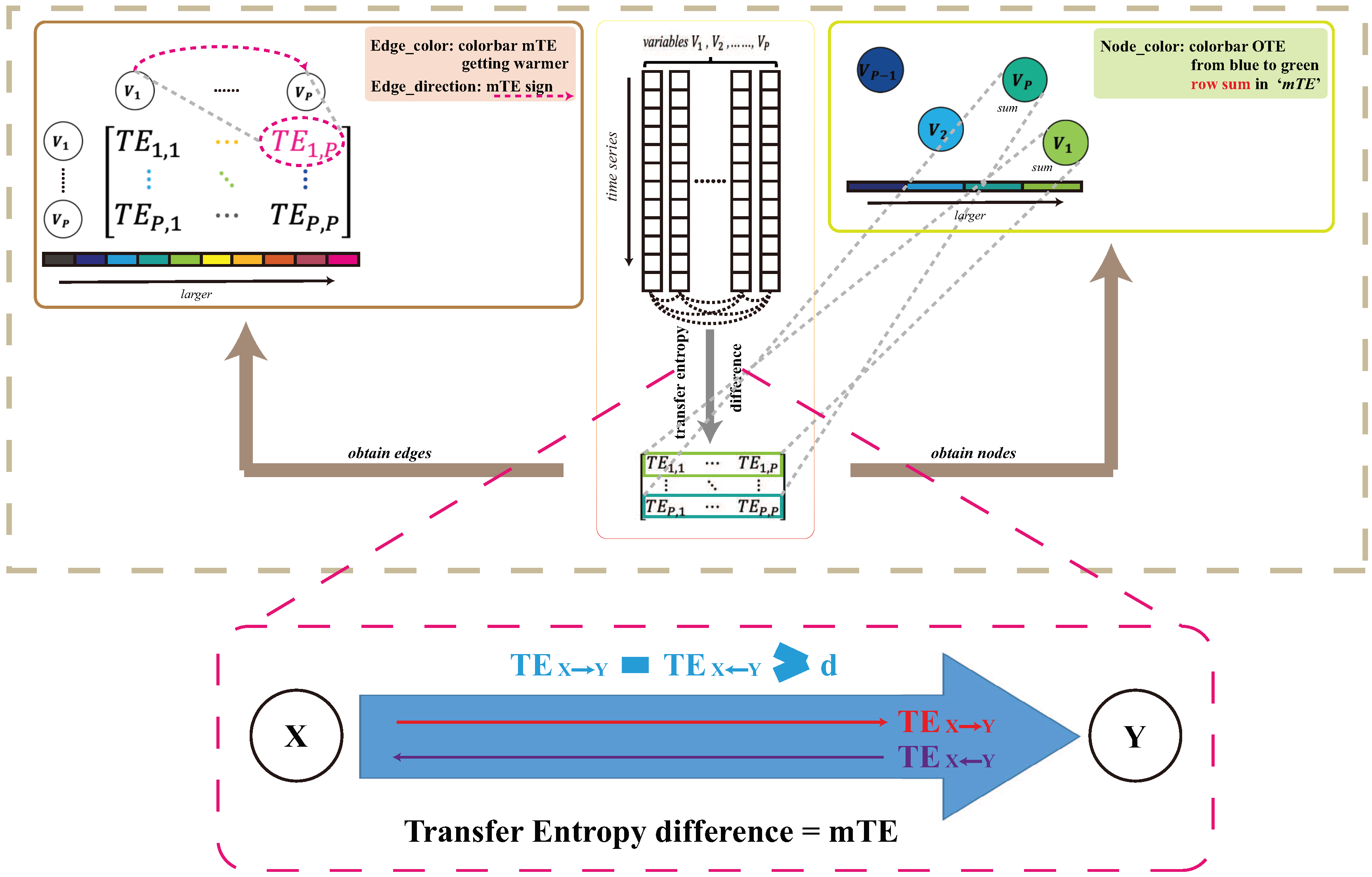
The proposed TE network inference model, that can be used for variable functional discovery and prediction at multiple scales, is explained. Its structure is graphically shown in Figure 2A.
2.1. Datasets
The Florida International University Southeast Environmental Research Center (FIU SERC) established a water quality monitoring system of 28 spatially distributed stations in Florida Bay, where each station (considered as a node in a network perspective) collects monthly data on Chlorophyll-a (CHLa), total organic carbon, inorganic and organic nitrogen and phosphorus (TN&TP), turbidity (TURB), pH, salinity (SAL), water temperature (TEMP), and dissolved oxygen (Boyer and Briceno, 2007; Nelson et al., 2017). CHLa has often been used as an indicator of blooms given its sensitivity to environmental changes, ease of monitoring, and ability to reflect phytoplankton biomass effectively (Boyer et al., 2009), but has not yet been verified as a systemic indicator of ecosystem health related to ecosystem function. We used a threshold-based quantile regression method (analogous to Nelson et al. (2017)) to establish an average threshold of on CHLa, universally applied to all stations, to distinguish bloom from non-bloom states across all stations. Initially, the dataset for this study spanned 2004 to 2006, corresponding to before, during, and after a severe bloom outbreak in Florida Bay in 2005 (Cloern and Jassby, 2010) in terms of CHLa extreme. In 1999 several blooms were observed in the same area but with lower CHLa extremes (Nelson et al., 2017). Then, the dataset (comprising all 2004, 2005, and 2006 CHLa monthly data) was filtered to include only those months and stations with CHLa values exceeding the critical blooming threshold, i.e., those months and stations indicating sustained bloom conditions. As a result, the final dataset contained 18, 63, and 136 rows of measurements (i.e., months) for the 2004, 2005, and 2006 bloom periods (pre- while-, and post-bloom), respectively. More generically, 2005 can be considered as epitomic of bloom outbreaks, while 2004 and 2006 are representative of early- and post-bloom periods.
2.2. Ecosystem Organization and Connectome
The entropy of the ecosystem, manifesting the ecological disorganization in relation to CHLa variability, is dependent on the pdfs that affect TE calculated on of pdfs’ divergence and asynchronicity. TE variability of an area, or the whole system, can be decomposed into eco-environmental interactions (considering CHLa and environmental factors acting as determinants or effect of ecological imbalance) and ecological areal interactions underpinning bloom spread. This variability affects the organization propagation of CHLa (i.e., how randomly distributed CHLa is) and in a information-balance equation can be written as the spatio-temporal convolution of the aforementioned components composing the ecosystem connectome, i.e.:
where, X stands for all other environmental variables except for CHLa, and stands for the location of each area being monitored over the period t. The specific TE chose in Equation (2.1) is related to TE analytics and posed objectives, later to be specified. It should be noted that the time delay between eco-env factors in Equation (2.1) has been set to one due to the sub-monthly variability of CHLa and the resolution of the data. Equation (2.1) is focused CHLa patterns where networks are the backbone determinants of the ecological ”weave” (CHLa interconnected patterns) that can be potentially controlled. Space and time are the dimensions along which CHLa is considered, plus other dimensions along gradients of environmental features on which stress-response patterns and related features (e.g. early-warning signals and risk thresholds) can be derived. Networks that define sources, sinks, pathways and determinants to guide monitoring and environmental control for bloom prevention. In this paper we specifically analyze the spatial ecological corridors determining bloom spreading and direct interactions between CHLa and environmental factors to quantify environmental effects of ecological dysbiosis; Wang and Convertino (2023) focused instead of the whole set of biogeochemical interactions useful for forecasting expect for bloom spreading networks.
2.3. Eco-Environmental Network Inference
Transfer entropy (), constructed from information entropy (Shannon, 1948), measures the causal relationship between two asynchronous and divergent variables (expressed as time series) X and Y (in the bivariate form, yet not accounting for second-order indirect interactions) by quantifying the predictive information flow between them (Schreiber, 2000). Previously the TE-based model, called ”Optimal Information Flow” (in relation to the maximization of ecosystemic entropy to gather the largest information), was used to discover causal relationships in human and aquatic ecosystems, e.g., for bacteria (Galbraith and Convertino, 2021; Galbraith et al., 2022; Li and Convertino, 2019) and fish interactions (Li and Convertino, 2021a) and assess ecosystem health.
The information flow, and thus the predictive relationship between variables, is bi-directional. In this paper we took the form of bivariate TE (yet skipping interactions higher than the third-order that is our first modeling assumption considering the weakly third-order interactions between environmental factors (Convertino and Wang, 2022)) and calculated the difference between the pairwise information flows to identify the strongest causal factor, i.e. and (where X and Y can be either ecological such as CHLa, or environmental variables) as follows:
where and are values of variables X and Y at time (yet, month that is our second modeling assumption considering the fact CHLa values are very sensitive to past changes in the immediate past reflecting a Markovian dynamics (Convertino and Wang, 2022) but long-term increasing trend can lead to extreme CHLa shifts). and denote the histories of time-varying variables X and Y up to and , respectively. is the transfer entropy of time series variable X to Y, whereas indicates the transfer entropy of Y to X. In this study we considered only positive where CHLa and Y are all other environmental factors for eco-environmental feedback in Equation (2.1), and all where X and Y are both CHLa in two different nodes. Additionally, in the TE calculation we did not investigate the optimal time-delay between X and Y, nor the optimal set of factors that are predictive of CHL as in Li and Convertino (2021a), due to the fact that: (i) bloom eco-env feedback occur at scale lower than one month (at which data are available), and (ii) our interest into the whole systemic dynamics.
The unbounded causality matrix, or more precisely the predictive causality matrix TE unconstrained to any prediction of biodiversity patterns as in Li and Convertino (2021b), based on calculated TEs without the optimization of and predictive environmental factors of ecological patterns in an Optimal Information Flow perspective, can be constructed as follows:
where TE in indeed a difference of transfer entropies as in TEGNN (Duan et al., 2022) in contrast to OIF (Li and Convertino, 2021a). For each year, two networks were constructed, each defined by an underlying matrix of transfer entropy differences . One inferred matrix was a spatial network in which the 28 stations were nodes and the causal influence among them were the edges. The time series used to calculate the transfer entropy differences (Equation (2.2)) in this network were the time series of CHLa measurements at each station. The second inferred network was a water quality network, in which the nodes were the water quality factors (CHLa, TN, TP, SAL, TEMP, and TURB) and the edges were the causal influence among them. In this study, however, the causality matrix underlying the water quality network was further filtered to focus only on the effect of CHLa on other water quality factors; the reverse effect of water quality factors on CHLa and the effect between water quality factors were not considered in this task. Following the Pareto principle (Sanders, 1987), the largest 20% values (and not 20% of events) should identify the most influential variables (stations or factors). Therefore, we only retained the largest 20% values in the in order to focus on the most influential variables.
where d is the threshold value, or Pareto critical value, of the significant causal relationship. If , then X is a significant cause of Y; otherwise X is a weak cause of Y, or X and Y are mutually causal without any preferential direction in causality (Equation (2.4) & Figure 2). Additionally, the values in the matrices for each of the three years were normalized to enable better comparison of the inferred interactions.
2.4. Eco-Environmental Factor Predictive Causality
The total Outgoing Transfer Entropy (OTE as in Galbraith et al. (2022) reflecting the total direct influence of one variable for all other influenced variables) of a node can be used to measure its influence on the collective dynamics (Equation (2.5)) as follows:
where OTE is the sum of the row in the matrix (after the application of the threshold as in Equation (2.4)). The larger OTE, the stronger the influence of node X on all other directly connected nodes in the network. In a information-balance perspective OTE is the cumulative effect of all environmental or ecological variables for a node.
3. Results and Discussion
3.1. Spatio-temporal Spreading and Fluctuations
To characterize and model the spreading of blooms we considered Florida Bay blooms in between 2004 and 2006. We novelly inferred a spatial influence network, underpinning bloom spread, among a set of spatially distributed water monitoring stations. This was achieved by deriving a TE matrix from spatio-temporal patterns of CHLa derived from monitored stations (see Section 2.3). The TE matrix for 2004 suggested that the study site was free of severe blooms, except for a few stations in the northwest: specifically, stations 16, 14, 25, and 26 (Figure 1) at least in 2004 where the resurgence of blooms was observed after the big bloom in 1999 (Convertino and Wang, 2022; Nelson et al., 2017).
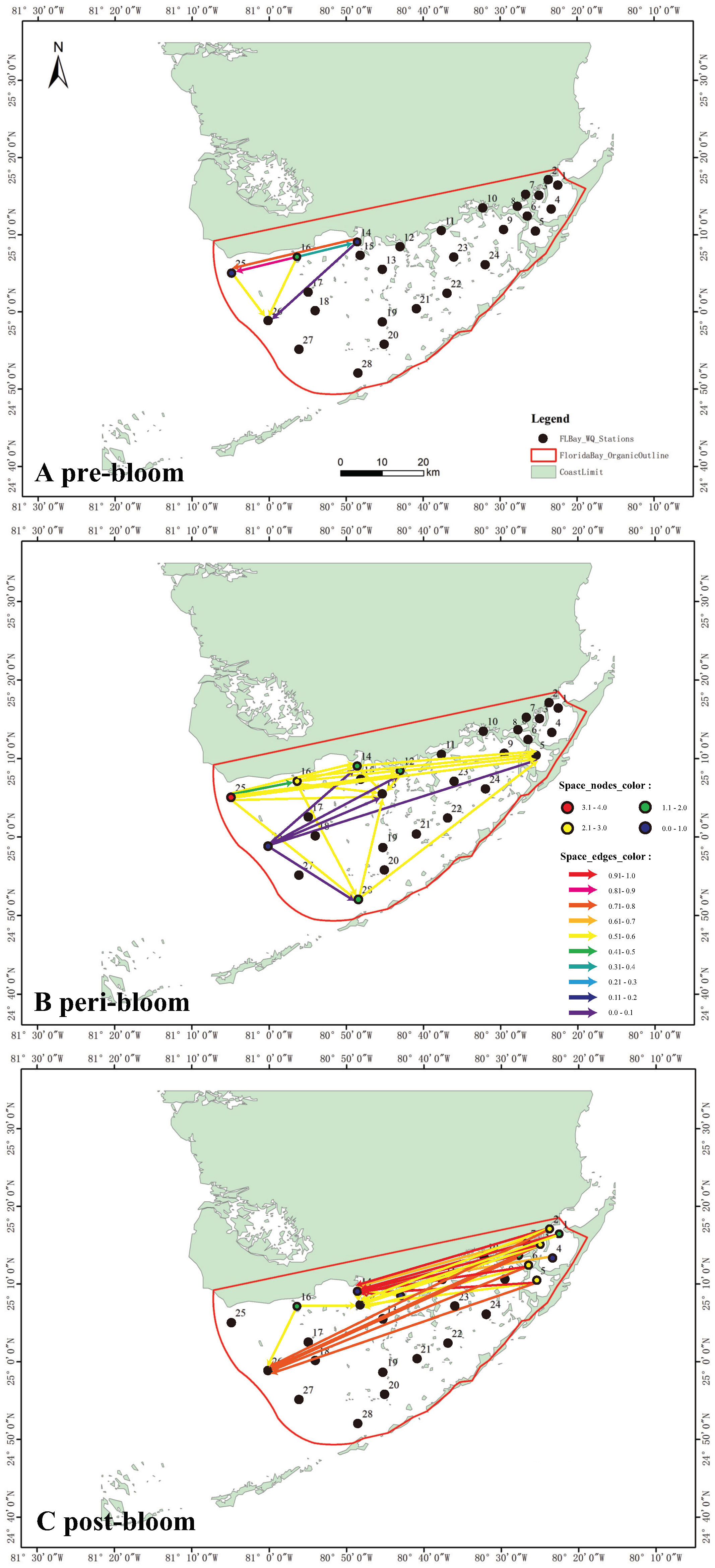
The properties of network edges, representing eco-environmental interactions, depend on (Equation (2.4)). The edge directions of the spreading network (Figure 3) suggested that an algal bloom would have initiated around station 16 and then move west with a preferential direction toward northwest.The edge colors (proportional to ) suggested that the bloom was moderately strong but localized in 2004 (Figure 3A) with a high probability to continue growing in the Bay (due to directions). The spatial spreading matrix for 2005 revealed large and widespread bloom outbreaks, concentrated in the western and central areas of the Bay (Figure 3B). In that year, the spatial influence was the strongest near stations 25, 16, 14, and 12 in the northwest and station 28 in the south region. The edge colors indicate that the bloom at all stations was moderately strong and also very likely to continue in the NE direction. Station 28 seems largely affected by many other stations in the bloom spreading, and yet likely a sink node with potentially strong ecological effects also considering its proximity to the FL coral reef. The matrix for 2006 (Figure 3C), showed the most extreme area interactions as well as a reversal in the spreading of blooms, i.e. moving from NE to central areas. The edge colors implied that bloom activity was extremely high, covering a wide area of Florida Bay. Nonetheless, the resulting graph suggested that after the largest outbreak the bloom moved from the easternmost into the north-central area, while the bloom in the west region had dissipated.
Figure 1.
Florida Bay and Area Classification based on CHLa dynamics. The red-blue classification in plot A is related to the probabilistic structure of CHLa as highlighted in plot B. Plot A also highlights the main habitats and species present in FL Bay.
Figure 1.
Florida Bay and Area Classification based on CHLa dynamics. The red-blue classification in plot A is related to the probabilistic structure of CHLa as highlighted in plot B. Plot A also highlights the main habitats and species present in FL Bay.
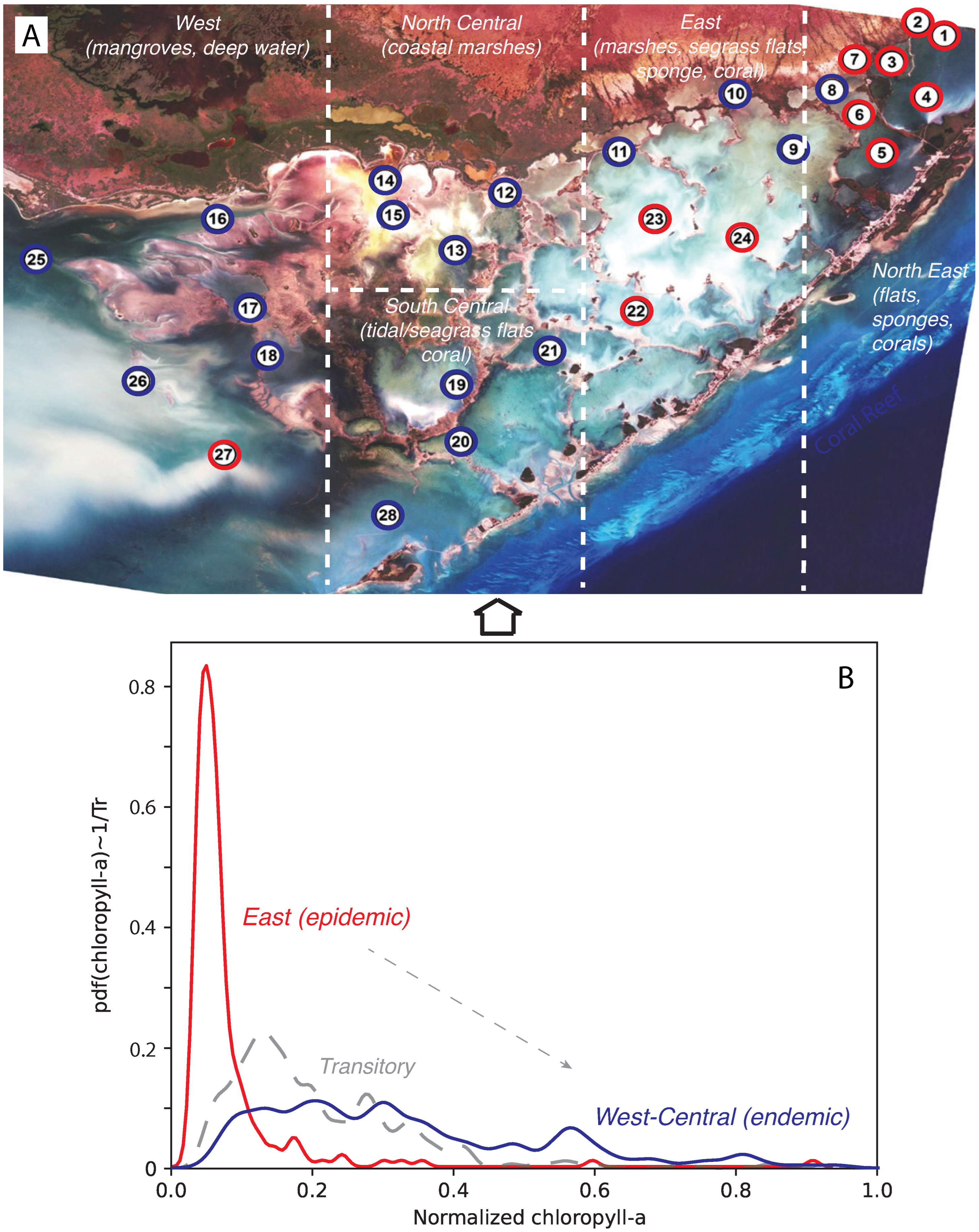
Figure 2.
Inference Model. The structure of the TE inference model. Here variables are annotated as V more generically. X can be thought as and Y all other environmental variables. Variable pairwise interactions and node collective influence (OTE) are determined via Equations (2.4) and (2.5), respectively.
We showed how by analyzing information flow among spatially distributed nodes, it is possible to model the spatial spread of a phenomenon, like algal blooms. In addition, this approach is able to detect sources, sinks, directions and salient pathways of bloom spreading. Due to various unaccounted factors such as wind intensity and direction, current direction, and bathymetry to name a few, there is a certain dynamic spatial change of blooms that is not attributed to the aforementioned factors. However, the model can take into account any environmental factor if available and yet it can attribute the degree of variability of CHLa. In a complex network sense, the bloom spatial network in 2004 is small in scale and regular in topology but has an obvious active station (station 16) that is an actively connected hub for bloom spreading. Therefore it is much easier to take measures against blooms at this time (whether possible) or to prevent triggers by controlling environmental determinants. This area is well-know to be heavily influenced by nutrient efflux from the Everglades (Nelson et al., 2017). Particularly with the outbreaks of blooms in 2005, and later in 2006 the network has many more area that are very active and affected, yet blooms management becomes more difficult. Over time a spreading network transition is observed from a regular/Small-World in 2004, to Scale-Free in 2005, and Regular (or uniform) topology in 2006 with long-range connections.
Figure 3.
Inferred spatial CHLa for 2004, 2005 and 2006 pre-, peri- and post-bloom periods in Florida Bay. Link and node color (from blue to red) is proportional to mTE based on CHLa interdependence between node pairs, and OTE considering only where Env stands for all other environmental factors. East to West node and link dynamic increase is observed from 2004 to 2006 as well as a spreading network transition from regular/Small-World to Scale-Free and Regular (or uniform) with long-range connections for 2004, ’05 and ’06. Each year corresponds to different bloom precursor area and environmental factors (Central and North-West more affected by nutrients), widespread and extremely localized outbreak (North-East more affected by temperature and turbidity and sequential effects of spreading).
3.2. Water Quality Trends and Bloom Impacts
The investigation of the impact of CHLa extremes (magnitude, duration and frequency) on ecosystem health is a poorly covered topic in science. To explore how algal blooms impacted water quality in Florida Bay, we analyzed how CHLa impact other water quality variables using TE (see Section 2.3). We focused our analysis on how CHLa implicated potential changes in water quality – in terms of predictive causality – for stations where extreme blooms were most likely. At the most active station in 2004 (i.e., station 16 characterized by coastal marshes that is likely the source of blooms; see Figure 3A blooms did not affect TN, TP, SAL, and TURB, except for a slight effect on water temperature (see Figure 4A). Rather, TN, TP, SAL, and TURB, likely driven by riverine efflux in the Bay, triggered CHLa changes leading to blooms as highlighted in Wang and Convertino (2023) and Convertino and Wang (2022). In 2005, the impact of blooms on other water quality factors was mostly evident at station 25 that is a deep-water mangrove habitat, where the blooms were the most intense (see Figure 3B). CHLa induced not only water temperature changes but also variations into total nitrogen and salinity (TN and SAL) with higher impact for the latter (Figure 4B). In 2006 (see Figure 3C) where blooms are the most extreme but localized (NW area), the effect of blooms on water quality peaked at station 3, followed by stations 5 and 2, and then station 6 in terms of magnitude (Figure 4C). Stations 2, 3, experienced blooms throughout the year, while station 6 had a relatively short blooms (7 months as reported in data). At stations 3 and 6 (characterized more by tidal flats) blooms induced changes in water temperature, salinity, total phosphorus, and turbidity, while at stations 2 and 5 (characterized more by submerged marshes) blooms led to substantial fluctuations in total nitrogen, total phosphorus, salinity, and turbidity. Information flow patterns (TE patterns) suggest that blooms are first strongly causing water temperature alterations, then enhancing salinity and nitrogen, and later impacting other nutrients (phosphorous) and turbidity. This is aligned to the understanding of underlying microbiological processes (Convertino and Wang, 2022). In the vicinity of station 2, blooms can cause a large change in salinity, while the effects on TN, TP, and TURB are less significant. As blooms are a manifestation of eutrophication in water bodies, large amounts of phytoplankton cause dramatic changes in the total phosphorus and turbidity such as near station 3, with minor influence on temperature and salinity. Around station 5, the bloom had a strong influence on turbidity and salinity, with minor impact on TN and TP due to the deeper water in this area. Despite bloom near station 6 is relatively short, it still caused elevated changes on both salinity and turbidity and in a minor way on water temperature and total phosphorus. In general, the occurrence of blooms had a serious effect on total phosphorus, salinity, and turbidity in the eastern zone of Florida Bay; a worrisome condition because of the highly valuable biodiversity in that area comprising a wide set of sponge, fish and coral species. Our results reveal that algal bloom severity also cause environmental degradation a-posteriori beyond the direct causal effect of environmental change (particularly from temperature in the ocean, and nutrients form estuarine efflux) in triggering blooms a-priori.
3.3. Bloom Intensity and Area Dependency
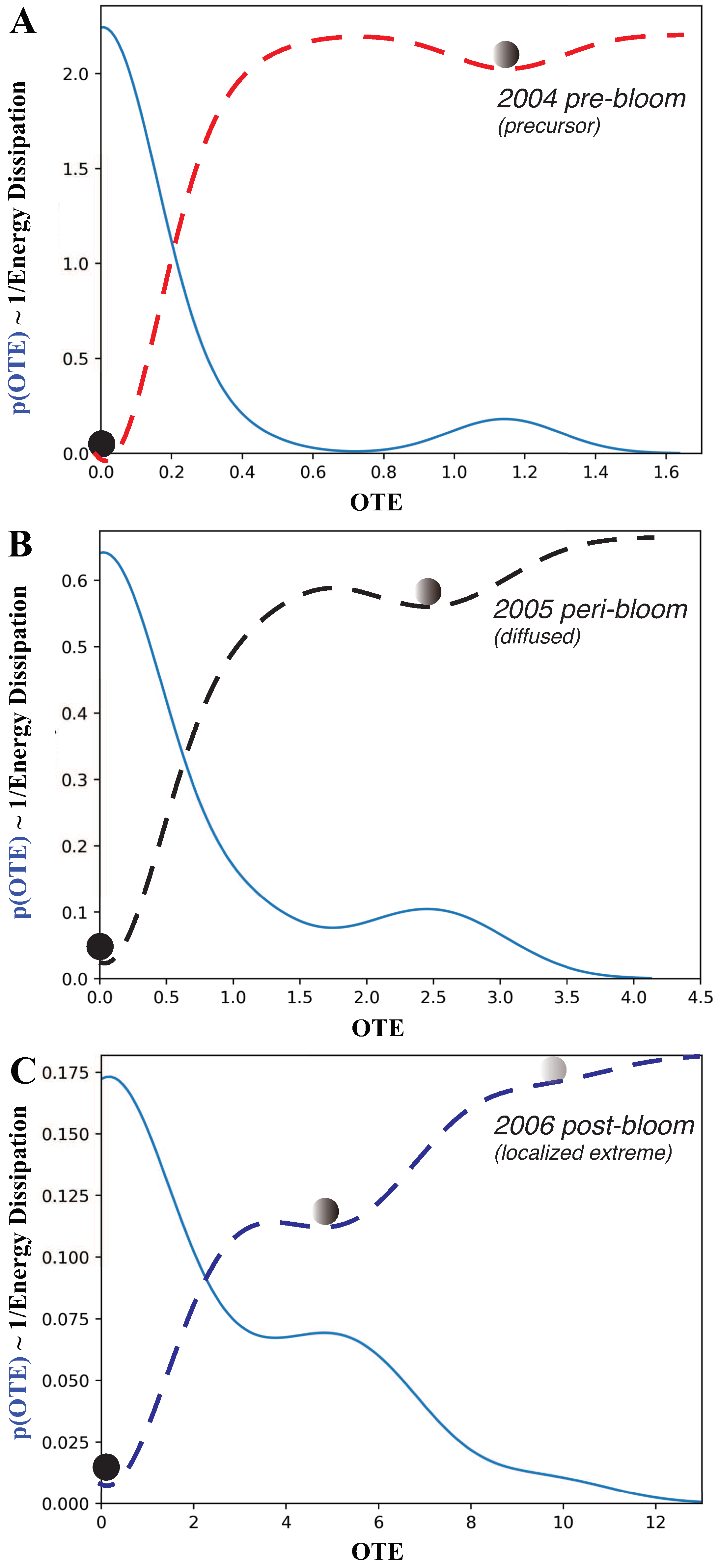
We explored the interaction dynamics of blooms by analyzing the annual probability distribution, or pdf, of Outgoing Transfer Entropy (OTE, see Figure 5) pre-, while- and post-bloom. OTE quantified the extent to which blooms around one area can predict CHLa dynamics (in terms of value and distribution) in other areas: higher OTE values indicate higher area interactions, yet higher spreading and predictability. In 2004, the OTE ranged between 0 and 1.7; most of values with a non-zero probability were between 0 and 0.6. It can be seen that most of the stations have no bloom, resulting in a low probability of large values of OTE, but a high probability of low OTE. The pdf is bimodal with a leptokurtic character. In an ecological sense, the dynamics is characterized by highly localized blooms, and few traces of bloom emergence in other areas. Thus, the bloom spatial network system was relatively contained in 2004 and corresponding to a regular/small-world topology (Figure 3). This also corresponded to a simple low-TE dynamics of eco-environmental interactions (Figure 4). In 2005, the OTE range increased to a maximum of 4.0, with most of OTE having higher probability than in 2004. In 2006, the range of OTE increased even further to a maximum of 13, with all OTE values having higher probability. This also corresponded to a shift in the pdf to a more platykurtic; yet, highlighting more widespread and common bloom dynamics. From the perspective of complex networks, the number of nodes with large OTE values increased over time. This indicates that an explosive spread of blooms across FL Bay. Therefore the initial energy dissipation is higher over time. In 2005 the system is in an active and complex state, that makes the management of blooms extremely challenging. The 2006 pdf has higher entropy because more Poisson than all previous years.
The pdf of OTE proves that OTE reflects the probabilistic state of ecosystems with particular reference to algal blooms in this case. The higher the entropy the larger the effect of blooms and the higher the ecological effects; interestingly for FL Bay we notice the the highest the entropy the more scale-free the bloom spreading network although a time-delay may exists between ecological effects (CHLa that is more random like in 2006) and the largest spreading network (that is in 2005) signifying potential long-term effects. By flipping the pdf it is possible to get information on the ecosystem potential landscape informing about energy dissipation, likelihood of shifts and relative stability of bloom conditions (Figure 5). The energy dissipation of the system, that is the potential amount of energy consumed by ecological processes, is visualized and , and scales with , therefore the higher the leptokurtic character of the pdf the lower the energy dissipation (such as in 2004). The energy potential also gives the number of ecological states (metastable states are identified by the point where the pre- and post-curvature of the energy landscape diverges in sign; those are represented by the balls in Figure 5), the probability of a configuration to be stable (the lower the energy potential with respect to all other states the higher the stability) and the likely shifts among states (proportional to the slope of the energy potential), all of which define the ”resilience” of the ecosystem that is rapidity to bounce back to initial states. Higher entropy corresponds to higher energy dissipation in relation to larger and more random OTEs. This implies lower probability of CHLa stable states which are much closer to each other and increasing in number, yet implying higher likelihood of shifts, with larger ecological impacts. For FL Bay, the energy dissipation is also increasing in average value for pre-, while-, and post-bloom periods indicating a diminishing resilience and loss of complexity of the system; this also highlights the persistent effects of blooms despite their relative short duration.
4. Conclusions
Nature-Based Solutions as Nationally Determined Contributions.
Species, including eukaryotes at the microscale, operate in dynamical ecosystems where the ability to respond to changing environmental flows is paramount. An effective collective response, affecting the re-balancing of optimal environmental states, requires suitable information transfer among species and thus critically depends on the interaction network. This underpins the process of evolution toward low entropy states (characterized by scale-free distribution of CHLa for instance) (Hidalgo et al., 2014) as well as adaptation to new environmental pressure states, some of which can be undesired such as those with persistent blooms. In this paper, we highlight the central role of information as salient data about collective eco-environmental dynamics manifesting spreading patterns with large and persistent ecological effects. In particular we showed how CHLa patterns carry information of underpinning ecohydrological networks (and associated spreading factors such as nutrients) that support ecosystem function and services. More generally, the discovery and inference of the ecosystem connectome allows for assessment of ecosystem health, investigation of causal determinants, proximity to ecosystem shifts, and targeted ecohydrological controls. Further work will look into the precise quantification of critical thresholds as early-warning signals of environmental factors leading to blooms accounting for ecosystemic stress.
Specifically for FL Bay we highlighted the spatial trends and water quality impacts of blooms and demonstrated that blooms are a recurring and persistent phenomenon over long period of time with continuous outbreak in interdependent regions. Through spatial analysis of the bloom spreading networks, we showed how regions not previously involved in blooms (i.e. the highly biodiverse NE habitats) were caused by large imbalance of CHLa in the western and central blooms that were an important causal factor. Subsequently the first bloom outbreak, persistent and recurring blooms were observed for several NE areas with long-lasting environmental impacts on turbidity and salinity aggravated by temperature increase. The analysis of water quality factors showed that the occurrence of the bloom could only affect small fluctuations of temperature initially; however, with repeating outbreaks bloom spread affected more and more other biogeochemical factors that are hardly controllable systemically. This implies that blooms management should start from the source, otherwise its impact will gradually expand and become uncontrollable, affecting also ecosystem stability and resilience and settling them into undesired ecological states. From the perspective of complex networks, this bloom event (2004-2006) evolved from a spatial network with a localized trigger area and a small-world topology to a random topology with long-range spatial diffusion. In 2005, where most stations were blooming, the spatial spreading network was scale-free (theoretically optimal in a purely topological and predictive sense (Martinello et al., 2017; Xu et al., 2023)) with a more random biogeochemical network (topologically suboptimal), that underpins the dichotomy between structural and functional networks for ecological risks.
Although the intensity, duration, and spatial distribution of blooms are governed by a multiplicity of factors, CHLa variability has still a wide degree of predictability and control in an ecosystem perspective considering both predictive and ecological engineering models. Our proposed spatial network and water quality inference model provides valuable suggestions for forecasting and management of blooms; for instance by pinpointing monitoring and nature-based solutions on source areas such as coastal blue-carbon habitats to inhibit progressive eco-environmental impacts.
Author Contributions
M.C. designed and guided the study, wrote and finalized the manuscript. H.W. performed the calculations and created the first figures and draft. E.G. helped in the writing of the the paper.
Acknowledgments
M.C. acknowledges the Shenzhen Peacock Pengcheng Talents funding (B class) and the Tsinghua SIGS start-up funding.
References
- Albert, Réka and Albert-László Barabási. 2002. Statistical mechanics of complex networks. Reviews of modern physics 74(1), 47. [CrossRef]
- Andrade Jr, José S, Hans J Herrmann, Roberto FS Andrade, and Luciano R Da Silva. 2005. Apollonian networks: Simultaneously scale-free, small world, euclidean, space filling, and with matching graphs. Physical review letters 94(1), 018702.
- Boccaletti, Stefano, Vito Latora, Yamir Moreno, Martin Chavez, and D-U Hwang. 2006. Complex networks: Structure and dynamics. Physics reports 424(4-5), 175–308. [CrossRef]
- Boyer, Joseph N and Henry O Briceño. 2007. South florida coastal water quality monitoring network. FY2006 Cumulative Report South Florida Water Management District, Southeast Environmental Research Center, Florida International University (http://serc.fiu.edu/wqmnetwork/).
- Boyer, Joseph N, Christopher R Kelble, Peter B Ortner, and David T Rudnick. 2009. Phytoplankton bloom status: Chlorophyll a biomass as an indicator of water quality condition in the southern estuaries of florida, usa. Ecological indicators 9(6), S56–S67. [CrossRef]
- Briceño, Henry O and Joseph N Boyer. 2010. Climatic controls on phytoplankton biomass in a sub-tropical estuary, florida bay, usa. Estuaries and Coasts 33(2), 541–553. [CrossRef]
- Burd, Adrian B and George A Jackson. 2002. An analysis of water column distributions in florida bay. Estuaries 25(4), 570–585. [CrossRef]
- Butler IV, Mark J, John H Hunt, William F Herrnkind, Michael J Childress, Rodney Bertelsen, William Sharp, Thomas Matthews, Jennifer M Field, and Harold G Marshall. 1995. Cascading disturbances in florida bay, usa: cyanobacteria blooms, sponge mortality, and implications for juvenile spiny lobsters panulirus argus. Marine Ecology Progress Series 129, 119–125. [CrossRef]
- Cloern, James E and Alan D Jassby. 2010. Patterns and scales of phytoplankton variability in estuarine–coastal ecosystems. Estuaries and coasts 33(2), 230–241. [CrossRef]
- Convertino, M, A Reddy, Y Liu, and C Munoz-Zanzi. 2021. Eco-epidemiological scaling of leptospirosis: Vulnerability mapping and early warning forecasts. Science of The Total Environment 799, 149102. [CrossRef]
- Convertino, Matteo and L James Valverde Jr. 2019. Toward a pluralistic conception of resilience. Ecological Indicators 107, 105510. [CrossRef]
- Convertino, Matteo and Haojiong Wang. 2022. Envirome disorganization and ecological riskscapes: The algal bloom epitome. In Risk Assessment for Environmental Health, pp. 327–346. CRC Press.
- Coscia, Michele, Fosca Giannotti, and Dino Pedreschi. 2011. A classification for community discovery methods in complex networks. Statistical Analysis and Data Mining: The ASA Data Science Journal 4(5), 512–546.
- Cosper, Elizabeth M, William C Dennison, Edward J Carpenter, V Monica Bricelj, James G Mitchell, Susan H Kuenstner, David Colflesh, and Maynard Dewey. 1987. Recurrent and persistent brown tide blooms perturb coastal marine ecosystem. Estuaries 10(4), 284–290. [CrossRef]
- Costa, L da F, Francisco A Rodrigues, Gonzalo Travieso, and Paulino Ribeiro Villas Boas. 2007. Characterization of complex networks: A survey of measurements. Advances in physics 56(1), 167–242. [CrossRef]
- Donges, Jonathan F, Yong Zou, Norbert Marwan, and Jürgen Kurths. 2009. Complex networks in climate dynamics. The European Physical Journal Special Topics 174(1), 157–179.
- Dorogovtsev, Sergey N, Alexander V Goltsev, and José Ferreira F Mendes. 2002. Pseudofractal scale-free web. Physical review E 65(6), 066122. [CrossRef]
- Duan, Ziheng, Haoyan Xu, Yida Huang, Jie Feng, and Yueyang Wang. 2022. Multivariate time series forecasting with transfer entropy graph. Tsinghua Science and Technology 28(1), 141–149. [CrossRef]
- Feldhoff, Jan H, Stefan Lange, Jan Volkholz, Jonathan F Donges, Jürgen Kurths, and Friedrich-Wilhelm Gerstengarbe. 2015. Complex networks for climate model evaluation with application to statistical versus dynamical modeling of south american climate. Climate dynamics 44(5), 1567–1581. [CrossRef]
- Galbraith, Elroy and Matteo Convertino. 2021. The eco-evo mandala: Simplifying bacterioplankton complexity into ecohealth signatures. Entropy 23(11), 1471. [CrossRef]
- Galbraith, Elroy, PR Frade, and Matteo Convertino. 2022. Metabolic shifts of oceans: Summoning bacterial interactions. Ecological Indicators 138, 108871. [CrossRef]
- Gfeller, D, P De Los Rios, A Caflisch, and F Rao. 2007. Complex network analysis of free-energy landscapes. Proceedings of the National Academy of Sciences 104(6), 1817–1822.
- Hidalgo, Jorge, Jacopo Grilli, Samir Suweis, Miguel A Munoz, Jayanth R Banavar, and Amos Maritan. 2014. Information-based fitness and the emergence of criticality in living systems. Proceedings of the National Academy of Sciences 111(28), 10095–10100. [CrossRef]
- Ilany, Amiyaal, Andrew S Booms, and Kay E Holekamp. 2015. Topological effects of network structure on long-term social network dynamics in a wild mammal. Ecology letters 18(7), 687–695. [CrossRef]
- Kumar, Ravi, Prabhakar Raghavan, Sridhar Rajagopalan, D Sivakumar, Andrew Tomkins, and Eli Upfal. 2000. Stochastic models for the web graph. In Proceedings 41st Annual Symposium on Foundations of Computer Science, pp. 57–65. IEEE.
- Li, Jie and Matteo Convertino. 2019. Optimal microbiome networks: macroecology and criticality. Entropy 21(5), 506. [CrossRef]
- Li, Jie and Matteo Convertino. 2021a. Inferring ecosystem networks as information flows. Scientific reports 11(1), 1–22. [CrossRef]
- Li, Jie and Matteo Convertino. 2021b. Temperature increase drives critical slowing down of fish ecosystems. PLoS One 16(10), e0246222. [CrossRef]
- Lin, Jingyi and Yifang Ban. 2013. Complex network topology of transportation systems. Transport reviews 33(6), 658–685. [CrossRef]
- Lotze, Heike K, Boris Worm, and Ulrich Sommer. 2000. Propagule banks, herbivory and nutrient supply control population development and dominance patterns in macroalgal blooms. Oikos 89(1), 46–58. [CrossRef]
- Martinello, Matteo, Jorge Hidalgo, Amos Maritan, Serena Di Santo, Dietmar Plenz, and Miguel A Muñoz. 2017. Neutral theory and scale-free neural dynamics. Physical Review X 7(4), 041071. [CrossRef]
- Nelson, Natalie G, Rafael Munoz-Carpena, and Edward J Phlips. 2017. A novel quantile method reveals spatiotemporal shifts in phytoplankton biomass descriptors between bloom and non-bloom conditions in a subtropical estuary. Marine Ecology Progress Series 567, 57–78. [CrossRef]
- Newman, Mark EJ. 2003. The structure and function of complex networks. SIAM review 45(2), 167–256. [CrossRef]
- Paerl, Hans W, Rolland S Fulton, Pia H Moisander, and Julianne Dyble. 2001. Harmful freshwater algal blooms, with an emphasis on cyanobacteria. TheScientificWorldJournal 1, 76–113. [CrossRef]
- Phlips, Edward J, Susan Badylak, and Tammy C Lynch. 1999. Blooms of the picoplanktonic cyanobacterium synechococcus in florida bay, a subtropical inner-shelf lagoon. Limnology and Oceanography 44(4), 1166–1175. [CrossRef]
- Reijneveld, Jaap C, Sophie C Ponten, Henk W Berendse, and Cornelis J Stam. 2007. The application of graph theoretical analysis to complex networks in the brain. Clinical neurophysiology 118(11), 2317–2331. [CrossRef]
- Sanders, Robert. 1987. The pareto principle: its use and abuse. Journal of Services Marketing 1(2), 37–40. [CrossRef]
- Schreiber, Thomas. 2000. Measuring information transfer. Physical review letters 85(2), 461. [CrossRef]
- Shannon, Claude Elwood. 1948. A mathematical theory of communication. The Bell system technical journal 27(3), 379–423.
- Smayda, Theodore J. 1997. What is a bloom? a commentary. Limnology and Oceanography 42(5part2), 1132–1136.
- Wang, H and M Convertino. 2023. Algal bloom ties: Systemic biogeochemical stress and chlorophyll-a shift forecasting. submitted –(–), –. [CrossRef]
- Wang, Xiao Fan. 2002. Complex networks: topology, dynamics and synchronization. International journal of bifurcation and chaos 12(05), 885–916.
- Xu, Li, Denis Patterson, Simon Asher Levin, and Jin Wang. 2023. Non-equilibrium early-warning signals for critical transitions in ecological systems. Proceedings of the National Academy of Sciences 120(5), e2218663120. [CrossRef]
- Zhang, Jie and Michael Small. 2006. Complex network from pseudoperiodic time series: Topology versus dynamics. Physical review letters 96(23), 238701. [CrossRef]
- Zhou, Changsong, Lucia Zemanová, Gorka Zamora, Claus C Hilgetag, and Jürgen Kurths. 2006. Hierarchical organization unveiled by functional connectivity in complex brain networks. Physical review letters 97(23), 238103. [CrossRef]
- Zhou, Changsong, Lucia Zemanová, Gorka Zamora-Lopez, Claus C Hilgetag, and Jürgen Kurths. 2007. Structure–function relationship in complex brain networks expressed by hierarchical synchronization. New Journal of Physics 9(6), 178. [CrossRef]
- Zou, Yong, Reik V Donner, Norbert Marwan, Jonathan F Donges, and Jürgen Kurths. 2019. Complex network approaches to nonlinear time series analysis. Physics Reports 787, 1–97. [CrossRef]
Figure 4.
Inferred biogeochemical networks for 2004, 2005 and 2006 pre-, peri- and post-bloom periods in Florida Bay. The purpose was to quantify local eco-environmental impacts for bloom sources. Yet, only four nodes in 2006, and one node for 2004 and 2005 were considered because those are the most active in terms of CHLa’s OTE. However, blooms are spreading phenomena and even other nodes are involved. Stations 16 and 25 are characterized by mangrove habitats in the West region, while stations 2, 3, 5 and 6 (displayed proportionally to a gradient of potential impact of CHLa on the environment) are characterized by coastal marshes and marine flat habitats in the East region of Florida Bay. The color of directed edges is proportional to ranges of mTE for only. The node color for CHLa is proportional to OTE while for other water quality factors depend on the frequency of local blooms during that year (yet, manifesting the potential impact of CHLa on the environment): specifically, blue, green, orange and pink are for 6, 7, 10, and 12 months of bloom occurrence.
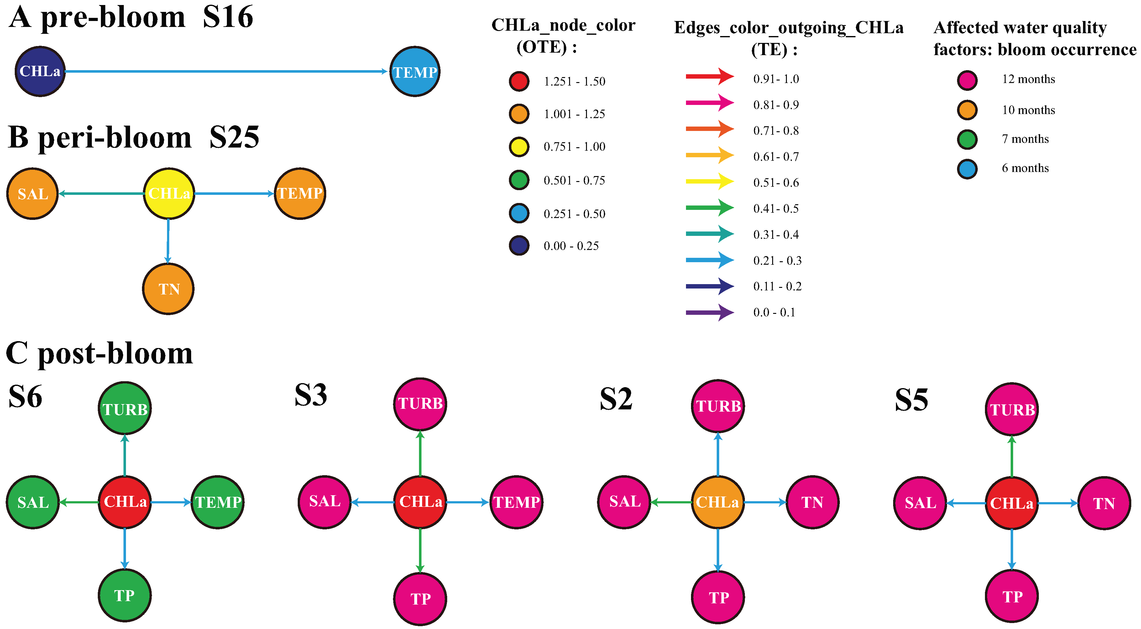
Figure 5.
Probability distribution of CHLa’s collective influence and ecosystem potential. A, B, and C are for 2004, 2005 and 2006 pre-, peri- and post-bloom periods in Florida Bay. CHLa’s collective influence is assessed based on OTE range and distribution, where the latter defines energy potential (in dashed red, black and blue for the 2004, 2005 and 2006 aligned to the distinct epidemic, transitory and endemic dynamics as in Figure 1B), stability of ecosystem states and transition probabilities from one to another.
Disclaimer/Publisher’s Note: The statements, opinions and data contained in all publications are solely those of the individual author(s) and contributor(s) and not of MDPI and/or the editor(s). MDPI and/or the editor(s) disclaim responsibility for any injury to people or property resulting from any ideas, methods, instructions or products referred to in the content. |
© 2023 by the authors. Licensee MDPI, Basel, Switzerland. This article is an open access article distributed under the terms and conditions of the Creative Commons Attribution (CC BY) license (http://creativecommons.org/licenses/by/4.0/).
Copyright: This open access article is published under a Creative Commons CC BY 4.0 license, which permit the free download, distribution, and reuse, provided that the author and preprint are cited in any reuse.


