1. Introduction
Most of vehicle crash investigations performed by some country transport departments certified that vehicle accidents are mostly caused by drivers who sometimes, when driving long distances, get tired and lose control, and then cannot manage the business of obstacle avoidance properly. The use of autonomous vehicles in general allows to reduce transport costs and can, in fast ways, avoid obstacles and then prevent accidents and thus save lives. Path planning of autonomous bicycles and study of their performances are subject to equilibrium constraints and create a lot of research questions, business and research opportunities. The study and the control of the dynamics of autonomous bicycles have become current and major concerns for the industrial operators and managers, and then attract the attention of research engineers, research mathematicians, research physicists, research computer scientists, etc. who develop suitable strategies, tools and methods to tackle and address all the problems associated to autonomous bicycles. There exists a considerable number of works on autonomous bicycles carried out since some years. Paper [
1] developed a bicycle robot with balancing control. Paper [
2] controlled the balance of a two-wheeled vehicle. Paper [
3] controlled a bicycle to illustrate the control of nonholonomic and under-actuated systems with symmetry. Paper [
4] designed and controlled a ball riding bicycle robot. Paper [
5] proposed a dynamical model for a bicycle. Book [
6] presents a different and unified perspective of the mechanics, planning and control of robots. The authors present the state of the art, the serew theoretic techniques which capture the most salient features of a robot in an intuitive way. Book [
7] provides fundamental notions on mobile robots, navigation, localization, manipulator-arm kinematics, dynamics, and point level control as well as camera modelling, image processing, feature extraction and multi-view geometry. Paper [
8] developed and analysed the kinematic and the dynamic models for a three wheeled bicycle called pedicab. Paper [
9] presented modelling and control strategies for an autonomous three wheeled mobile robot with front wheel steer and front wheel drive. Book [
10] provides a summary of common vehicle control systems and the dynamic models which are used to develop those control systems. All the above-mentioned papers are closely connected with the main subject of this paper because they deal in one way or another with control. To the best of my knowledge, none of those articles considered the control of an autonomous bicycle robot where the desired point is the rear Axle and uses optimal control theory methods. None of them computed the optimal state of the system, the corresponding costate functions and optimal speed . Generally it is noticeable that for other articles, before applying optimal control theory, the system is first reduced into a simpler one so that its characteristics can be determined easily. Most of time, the state system is linearized with respect to an equilibrium point, and inthose papers certain parameters are set in simpler values. The simplifications are performed to easily apply certain operations such as designing a quadratic regulator. However, when a nonlinear control system is reduced into a linear one, if no strategy is adopted, there will be loss of information, and then the final results will be considerably and significantly different from the exact ones. In this paper, the control system is highly nonlinear and has been studied as it is. No other paper has addressed the minimization of the running energy. No paper has computed the optimality conditions. No article has performed the derivation of a costate system of ordinary differential equations adjoining the state system. In the literature no paper found as considering the impact of the size of the initial costate vector on the length of the trajectory. So, most of the above-cited papers and others not cited addressed the bicycle stability problem, the tracking problem, etc., without considering the minimization of the running costs. This article is based on the control of the kinematics of a bicycle robot where the reference point is the center of the rear wheel. This paper uses optimal control theory to compute feasible control strategies of an autonomous bicycle and feasible state trajectories such that the bicycle running cost is minimize.
The main contributions of this paper are the design and computation of two feasible control strategies, the computation of the solution of the combined state-costate system of ordinary differential equations which is defined by six feasible state functions representing the feasible system responses to reference commands, six costate (adjoint) functions. To perform computation, scilab computer programs were developed and applied. This paper is organized as follows:
Section 2 develops different relevant mathematical models and formulates the problem as an optimal control problem.
Section 3 computes the system Hamiltonian, derives and solves the normal equations of optimality.
Section 4 applies Pontryagin’s Minimum Principle to derive all the relevant nonlinear ordinary differential equations.
Section 5 develops relevant computer programs in Scilab to compute the feasible control trajectories, the corresponding state and costate (adjoint) trajectories, the bicycle speed function and all the other outputs.
Section 6 designs the associated computational simulations.
2. Mathematical Models
2.1. Control System, Kinematic Model
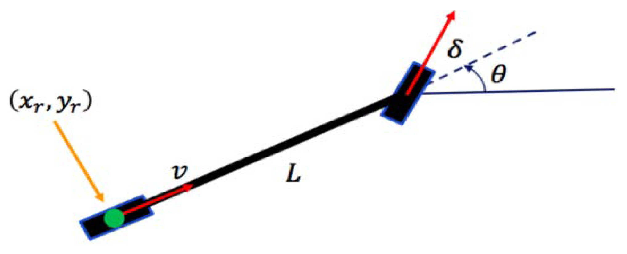
The reference point for the motion is at the centre of the rear-axle of the bicycle. The motion of an autonomous bicycle on the horizontal plane is modelled as follows:
where
and
are constant of proportionality,
and
are respectively the radius of the wheels and the distance between the centre of the rear and the front wheels.
are the coordinates of the projection of the rear-axle’s center (which is the reference point for the motion) on the horizontal plane,
is the heading angle,
is the steering angle,
is the steering angle’s velocity.
The reference commands which regulate the bicycle angular velocity and the steering angle velocity are modelled as solution to a closed-loop system defined by:
and are the unknown input control variables to be developed. and are constants of proportionality.
The whole robot kinematic control system is
Figure 1.
Rear-Axle Bicycle Robot Geometric Model.
Figure 1.
Rear-Axle Bicycle Robot Geometric Model.
2.2. Objective Functional
In this paper, the total running cost to be minimized is as follows:
where
and
are respectively the bicycle motion’s starting and final times,
and
are the reference commands which control respectively the bicycle angular velocity and steering angle velocity.
is called cost rate.
2.3. Problem Formulation
This paper addresses the following problem: Compute the feasible control strategies and the associated feasible state functions, also called feasible robot system responses, to bring the autonomous bicycle robot from a given initial state to a final state such that the total running cost is minimized.
3. Hamiltonian and Feasible Controls
The Hamiltonian of the system is given by
Where we have
is the energy cost rate,
is the x component of the linear velocity of the bicycle,
is the y component of the linear velocity of the bicycle,
is the rate of change of the heading angle of the bicycle,
is the rate of change of the steering angle of the bicycle,
is the rate of change of the bicycle angular velocity,
is the rate of change of the velocity of steering angle.
is the unkown state vector function. It is built to store all the state functions.
is the unkown costate (adjoint) vector function.
It is built to store all the costate functions. Concerning the control functions, the normal equations for optimality are as follows:
The feasible control functions are given by
4. Normal Condition for Optimality
If
is the optimal control of the above problem and
the corresponding optimal system response to the input control
, then there exists a costate vector function
, also called adjoint vector such that the following are satisfied:
By letting , with and for the control functions,
, , , , and for the state functions,
, , , , and for the costate functions
and by combining all the state and costate functions into a vector
, then the combined state-costate system can be rewritten as
Vector is built to vectorize the combined state and costate system of equations so that the system can be analyzed and processed in a easy and rigorous manner.
Notice that in the system (32)-(43) the right hand side and its gradient are continuous. Therefore, the solution exists and is unique.
5. Computer Program
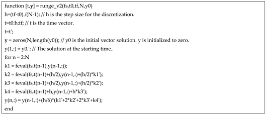
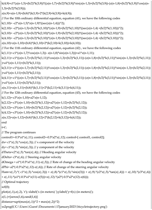
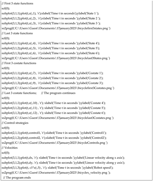
Pontryagin’s Minimum Principle applied in this article involves a costate system of ordinary differential equations which combined to the state system and the feasible controls gives a combined free-control state-costate system of ordinary differential equations. I order to solve any system of ordinary differential equations which is an initial value problem, I developed (in Matlab) an algorithm coding a fourth-order Runge-Kutta method. Such an algorithm can be translated into many other programming languages. It is as follows:
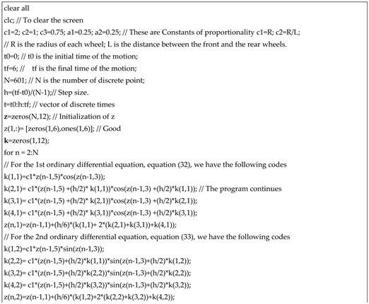
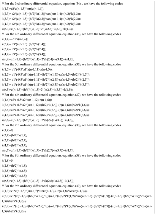
The above algorithm can be used to solve any initial value problem. Let’s use it to solve the system (32)-(43) of equations. By translating and developing the algorithm into Scilab codes we have the following set of codes:
6. Computational Simulations
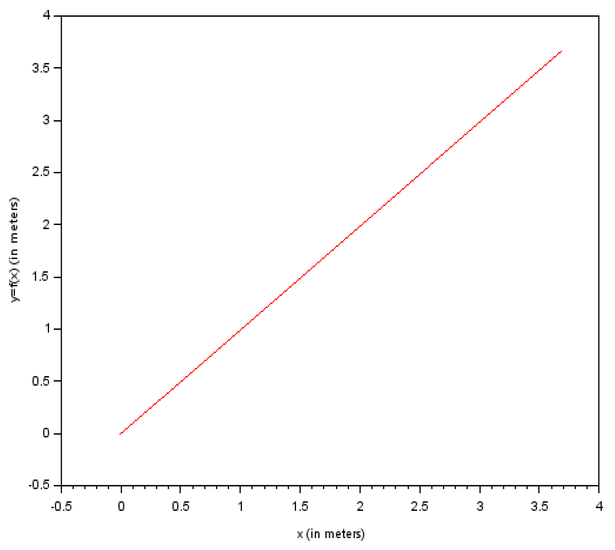
Figure 2 gives the feasible trajectory of the bicycle robot. The starting point of the path is (0,0).
Figure 2.
Feasible Bicycle Robot Trajectory.
Figure 2.
Feasible Bicycle Robot Trajectory.
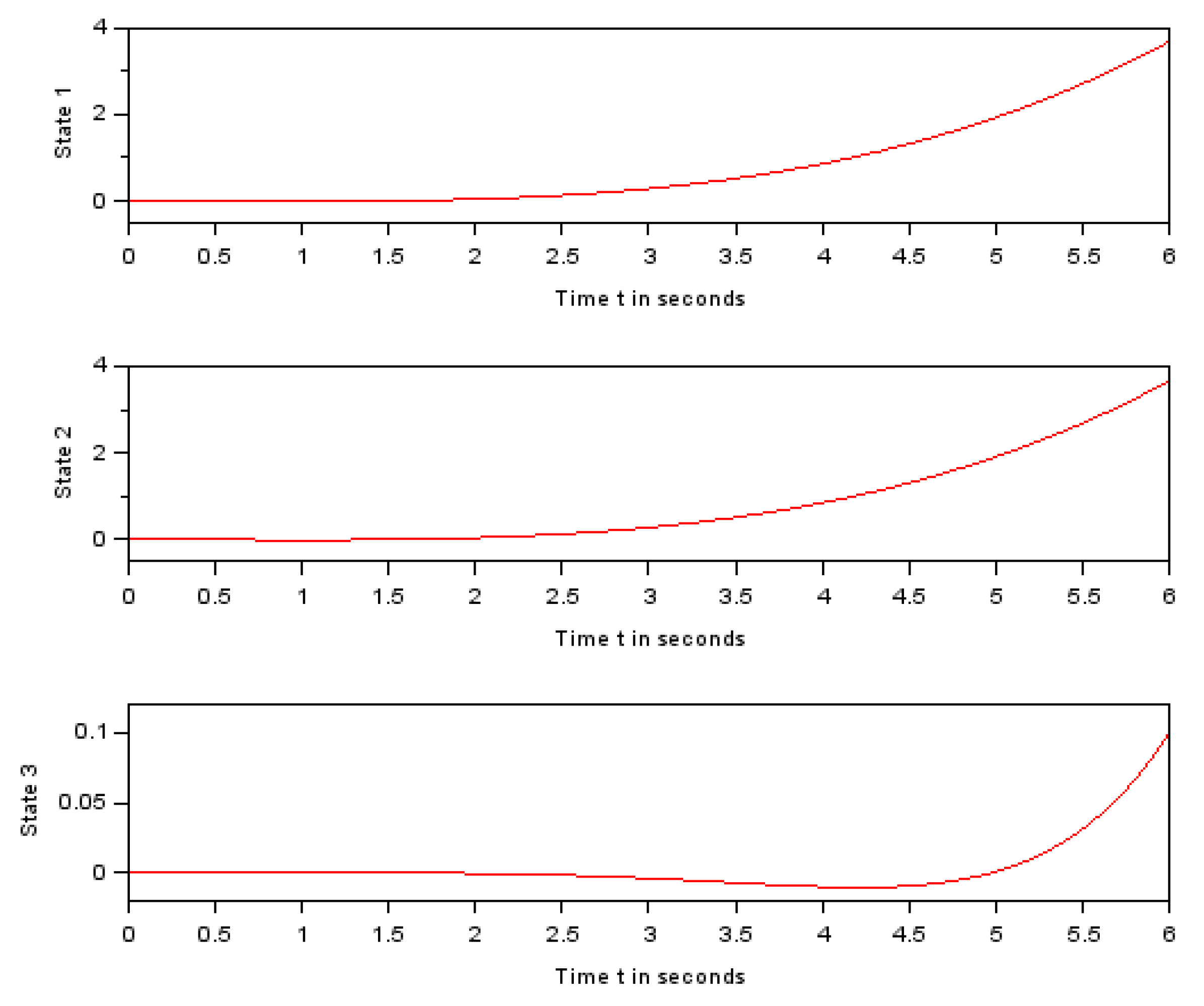
Figure 3.
First three feasible state functions.
Figure 3.
First three feasible state functions.
Figure 4.
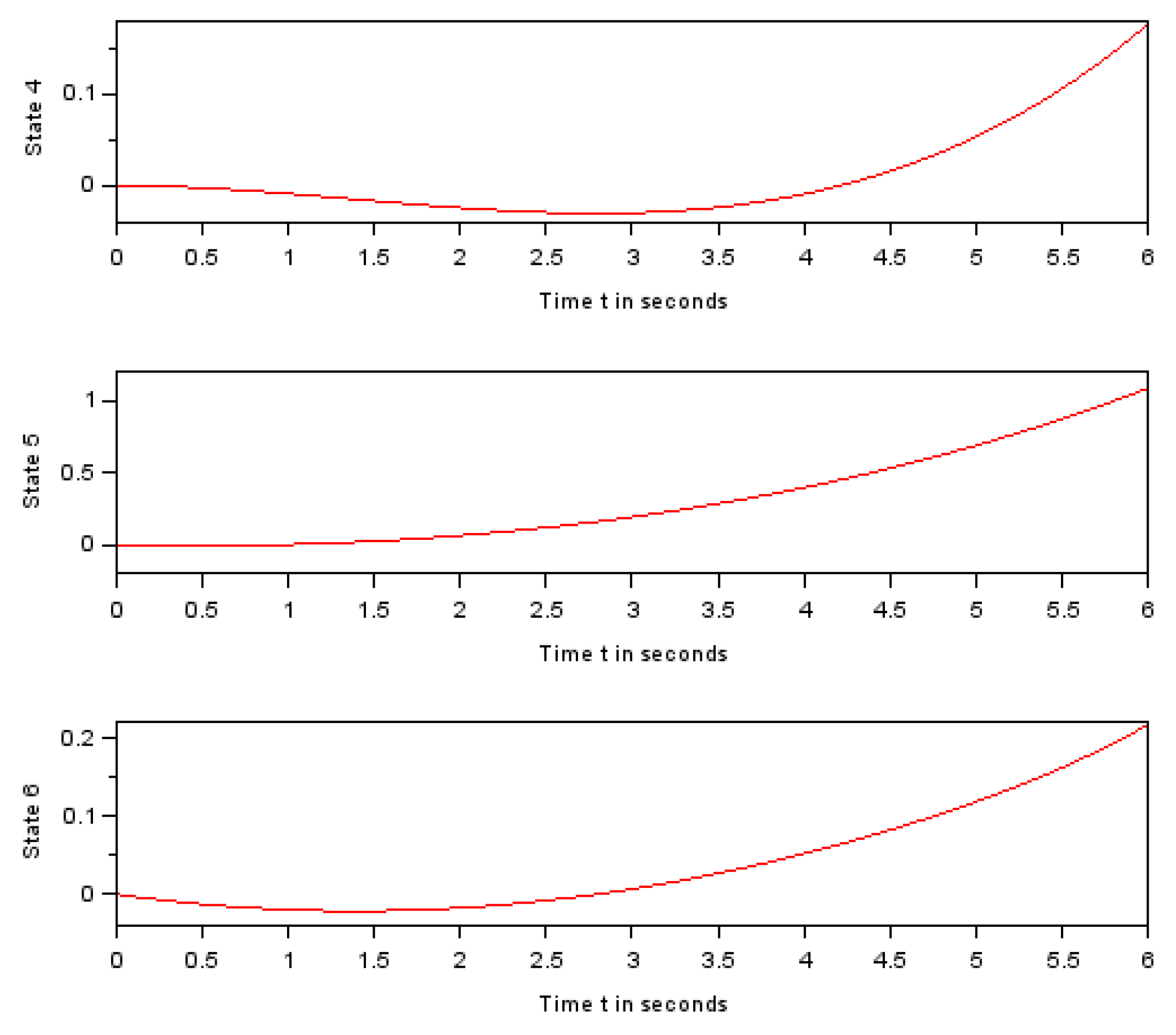
Last three feasible state functions.
Figure 4.
Last three feasible state functions.
The above plotted function describes the instantaneous robot’s position in the direction. In other words we have , . The above plotted function describes the instantaneous robot’s position in the direction. In other words we have , . The above plotted function describes the instantaneous robot’s heading angle. In other words we have , . The above plotted function describes the instantaneous steering angle. , . The above plotted function describes the instantaneous angular velocity. , . The above plotted function describes the instantaneous steering angle’s velocity. , .
Figure 5.
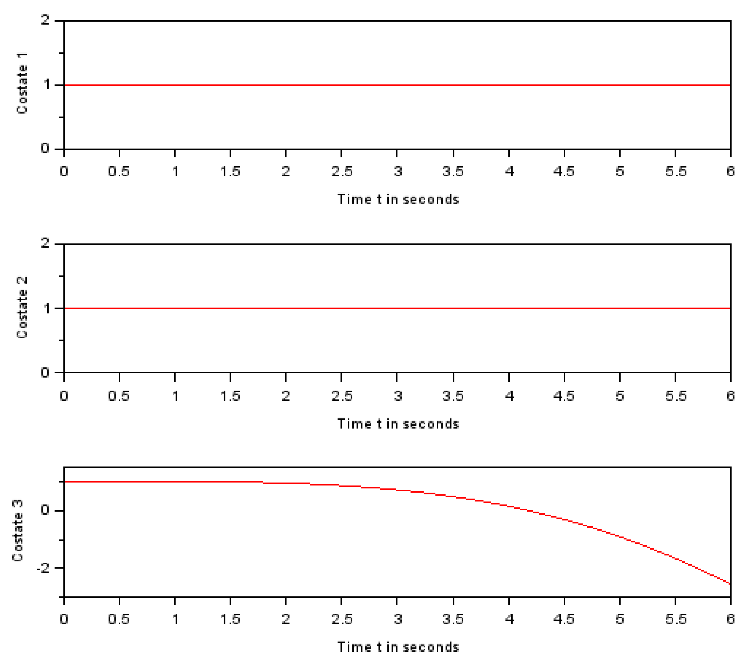
First three feasible costate functions.
Figure 5.
First three feasible costate functions.
Figure 6.
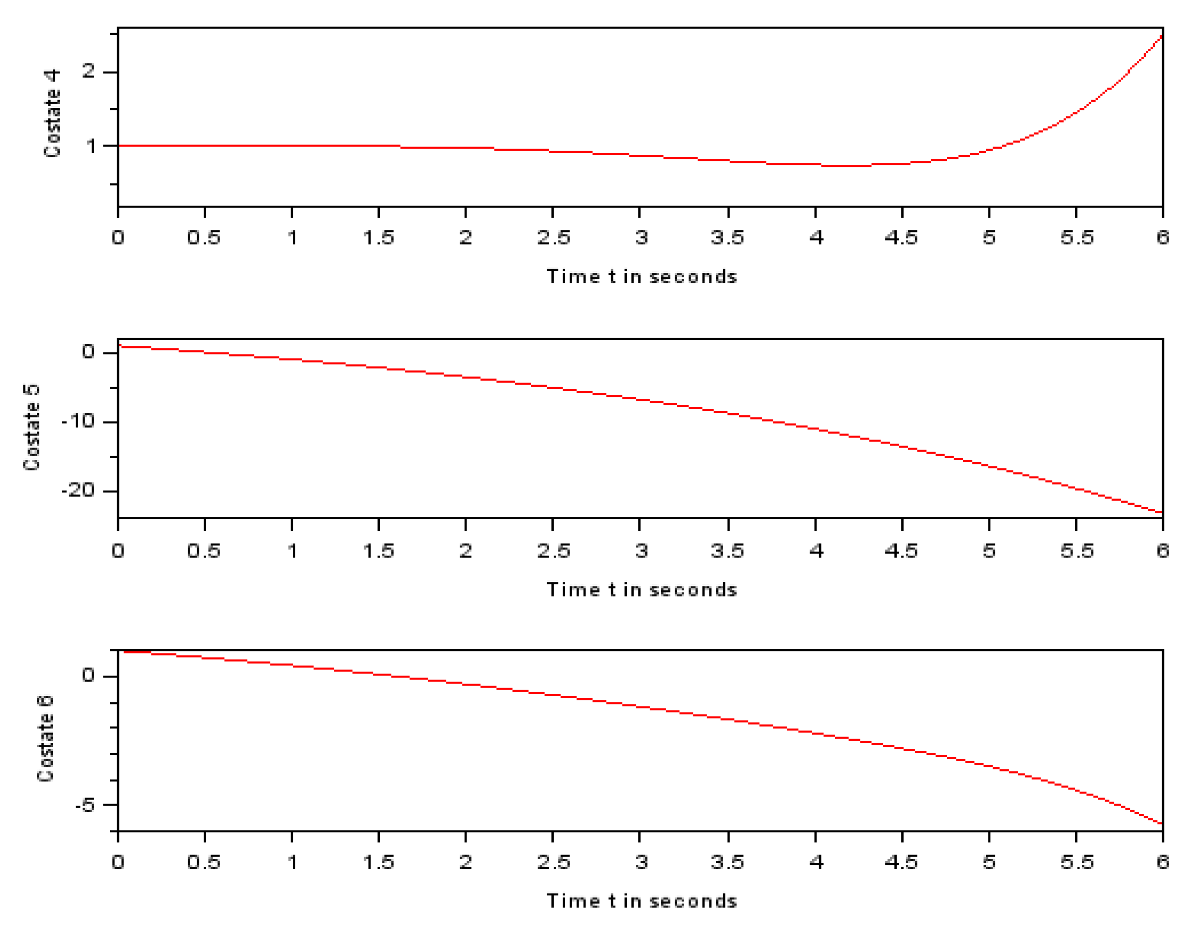
Last three feasible costate functions.
Figure 6.
Last three feasible costate functions.
The function is the adjoint function to the function . , . The function is the adjoint function to the function . , . The function is the adjoint function to the function . , . The function is the adjoint function to the function . , .
The function is the adjoint function to the function . , . The function is the adjoint function to the function . , .
One can notice that and are constant because their time derivatives are zeros.
Figure 7.
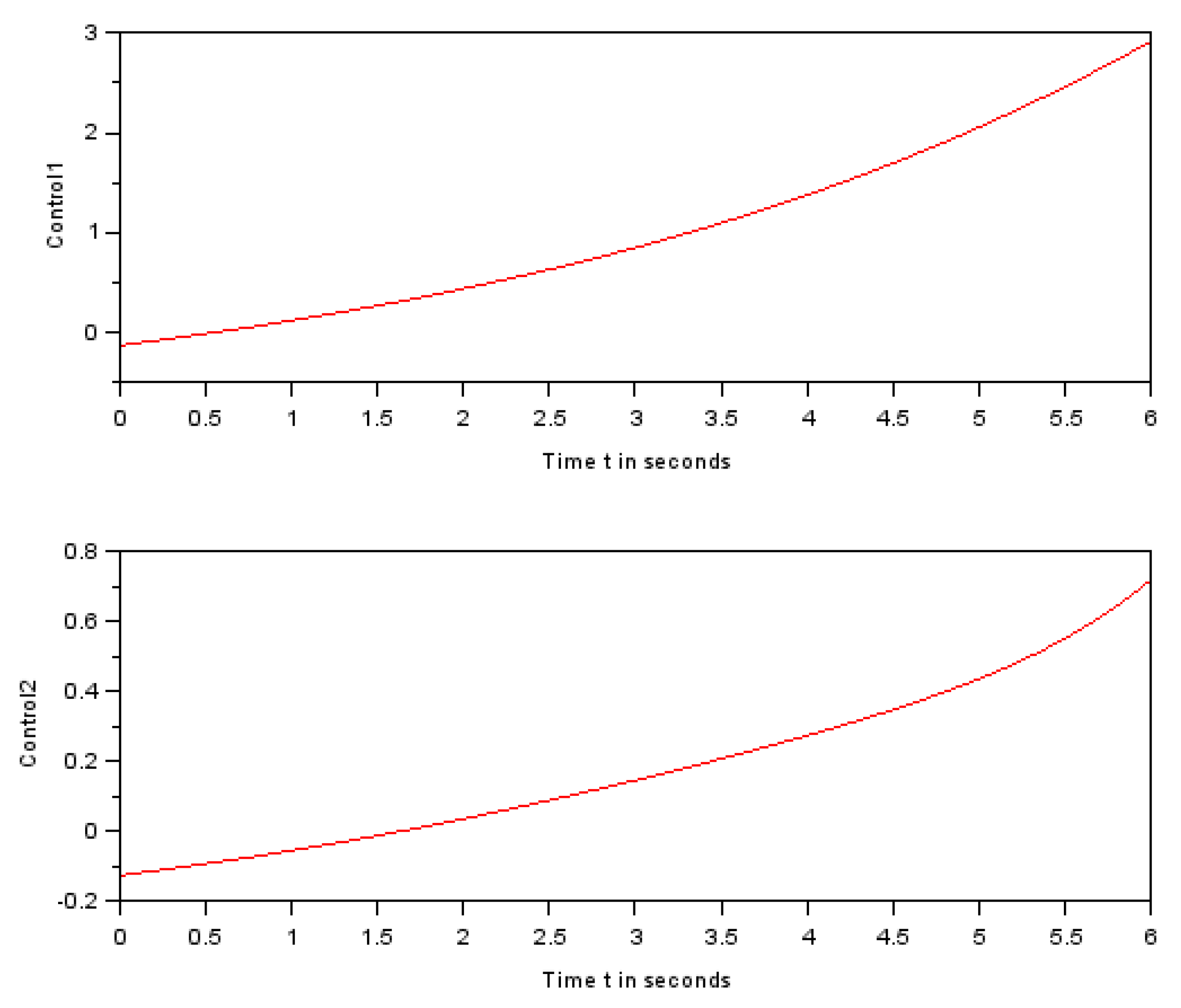
Feasible control strategies.
Figure 7.
Feasible control strategies.
The function describes the instantaneous reference command to the robot angular velocity. In other words we have . The function describes the instantaneous reference command to the robot angular velocity. In other words we have .
7. Conclusions
The aim of this paper was to compute the feasible control strategies and the associated feasible state functions, also called feasible robot system response to control, for an autonomous rear-axle bicycle robot to bring it from a given initial state to a final state such that the total running cost is minimized. A fourth-order Runge-Kutta was used to solve the combined free-control state-costate system of ordinary differential equations obtained from Pontryagin’s Minimum Principle. The obtained results enable to predict the performance of the autonomous bicycle robot so that it can be controlled accurately and efficiently. The computer programs are useful to any reader or any researcher who is familiar with programming and who would want to learn more. Computational Simulations are provided to show the effectiveness and the reliability of the approach. In future, control policies will be developed for the rear-axle bicycle robot to asymptotically track a prescribed trajectory. Some methodology will be performed to develop optimal control strategies using Lagrange Interpolating polynomial.
Funding
This research was funded by the University of Johannesburg, Faculty of Engineering through UJ-GES.
Data Availability Statement
This study did not report any data.
Acknowledgments
The authors of this paper thanks the university of Johannesburg for financial support. They thank also the reviewers for relevant and helpful comments.
Conflicts of Interest
The authors declare no conflict of interest.
References
- Anan Suebsomran, Balancing Control of Bicycle Robot (2012), 2012 IEEE International Conference on cyber technology in Automation, control and Intelligent Systems(Cyber), pp. 69-73. [CrossRef]
- Ngoc Kien Vu., Hong Quang Nguyen, Balancing control of a Two-wheeled bicycle (2020), Mathematical Problems in Engineering. Published by Hindawi. [CrossRef]
- Neil H. Getz, Jerrold E. Marsden, Control for an Autonomous Vehicle, Department of Electrical Engineering, University of California. Berkeley, CA 94720, getz@eecs.berkeley.edu.
- Pongsakorn Seekkao and Manukid Parnichkun, Development and control of a bicycle robot based on steering and pendulum balancing, Mechatronics, Volume 69, August 2020. [CrossRef]
- Y. Tanaka and T. Murakami, Self Sustaining Bicycle Robot with Steering Controller, Advanced Control, 2004 IEEE International Workshop on Advanced Control, 27-31 may 2012. [CrossRef]
- Lynch, Kevin M., and franck C. Park, Modern Robotics: Mechanics, Planning, and Control 1st edition, Cambridge Press, 2017.
- Corke, Peter I. Robotics, Vision and Control: Fundamental Algorithms in Matlab, Springer, 2011.
- Noverina, Nur Hamid, Grafika Jati, M. Anwar Ma’sum, Wisnu Jatmiko, Kinematics and Dynamics Analysis of an Autonomous Three-Wheeled Bicycle Modeling, 2019 4th Asia-Pacific Conference on Intelligent Robot Systems (Conference Paper), July 2019.
- Pandey, S. Jha, and D. Chakravarty, Modeling and Control of an autonomous three-wheeled mobile robot with front steer, Proceeding 2017 1st Conference on Robot and Computing. IRC 2017, pp. 136-142, 2017. [CrossRef]
- R. Rajamani, Vehicle Dynamics and Control, vol. Spec No. 2001.
|
Disclaimer/Publisher’s Note: The statements, opinions and data contained in all publications are solely those of the individual author(s) and contributor(s) and not of MDPI and/or the editor(s). MDPI and/or the editor(s) disclaim responsibility for any injury to people or property resulting from any ideas, methods, instructions or products referred to in the content. |
© 2023 by the authors. Licensee MDPI, Basel, Switzerland. This article is an open access article distributed under the terms and conditions of the Creative Commons Attribution (CC BY) license (http://creativecommons.org/licenses/by/4.0/).
