Bell's Theorem Begs the Question

I. Introduction

Some claims of impossibility proofs in physics are known to harbour unjustified assumptions. In this paper, I show that Bell’s theorem [1] against local hidden variable theories completing quantum mechanics is no exception. It is no different, in this respect, from von Neumann’s theorem against all hidden variable theories [2], or the Coleman-Mandula theorem overlooking the possibilities of supersymmetry [3]. The implicit and unjustified assumptions underlying the latter two theorems seemed so innocuous that they escaped notice for decades. By contrast, Bell’s theorem has faced skepticism and challenges by many from its very inception (cf. footnote 1 in [4]), including by me [4,5,6,7,8,9,10,11,12,13,14,15], because it depends on a number of questionable implicit and explicit physical assumptions that are not difficult to recognize [9,15]. In what follows, I bring out one such assumption and demonstrate that Bell’s theorem is based on a circular argument [8]. It unjustifiably assumes the additivity of expectation values for dispersion-free states of hidden variable theories for non-commuting observables involved in the Bell-test experiments [16], which is tautologous to assuming the bounds of $\pm 2$ on the Bell-CHSH sum of expectation values. It thus assumes in a different guise what it sets out to prove. As a result, what is ruled out by Bell-test experiments is not local realism but additivity of expectation values, which does not hold for non-commuting observables in dispersion-free states of hidden variable theories to begin with.

II. Heuristics for Completing Quantum Mechanics

The goal of any hidden variable theory [2,17,18] is to reproduce the statistical predictions encoded in the quantum states $|\psi \rangle \in \mathcal{H}$ of physical systems using hypothetical dispersion-free states $|\psi ,\lambda ):=\left\{\right|\psi \rangle ,\lambda \}\in \mathcal{H}\otimes \mathcal{L}$ that have no inherent statistical character, where the Hilbert space $\mathcal{H}$ is extended by the space $\mathcal{L}$ of hidden variables $\lambda$, which are hypothesized to “complete” the states of the physical systems as envisaged by Einstein [19]. If the values of $\lambda \in \mathcal{L}$ can be specified in advance, then the results of any measurements on a given physical system are uniquely determined.

To appreciate this, recall that expectation value of the square of any self-adjoint operator $\mathsf{\Omega }\in \mathcal{H}$ in a normalized quantum mechanical state $|\psi \rangle$ and the square of the expectation value of $\mathsf{\Omega }$ will not be equal to each other in general:

$$\langle \psi \left|{\mathsf{\Omega }}^2\right|\psi \rangle \ne {〈\psi \left|\mathsf{\Omega }\right|\psi 〉}^2.$$

(1)

This gives rise to inherent statistical uncertainty in the value of $\mathsf{\Omega }$, indicating that the state $|\psi \rangle$ is not dispersion-free:

$$\Delta \mathsf{\Omega }=\sqrt{\langle \psi \left|\right\{\mathsf{\Omega }-{\langle \psi \left|\mathsf{\Omega }\right|\psi \rangle \}}^2|\psi \rangle }\ne 0.$$

(2)

By contrast, in a normalized dispersion-free state $|\psi ,\lambda )$ of hidden variable theories formalized by von Neumann [2], the expectation value of $\mathsf{\Omega }$, by hypothesis, is equal to one of its eigenvalues $\omega \left(\lambda \right)$, determined by the hidden variables$\lambda$,

$$\left(\psi ,\lambda \left|\mathsf{\Omega }\right|\psi ,\lambda \right)=\omega \left(\lambda \right)⟺\mathsf{\Omega }|\psi ,\lambda )=\omega \left(\lambda \right)|\psi ,\lambda ),$$

(3)

so that a measurement of $\mathsf{\Omega }$ in the state $\left|\psi ,\lambda \right)$ would yield the result $\omega \left(\lambda \right)$ with certainty. How this can be accomplished in a dynamical theory of measurement process remains an open question [17]. But accepting the hypothesis (3) implies

$$(\psi ,\lambda |{\mathsf{\Omega }}^2|\psi ,\lambda )={(\psi ,\lambda |\mathsf{\Omega }|\psi ,\lambda )}^2.$$

(4)

Consequently, unlike in a quantum sate $|\psi \rangle$, in a dispersion-free state $|\psi ,\lambda )$ observables $\mathsf{\Omega }$ have no inherent uncertainty:

$$\Delta \mathsf{\Omega }=\sqrt{(\psi ,\lambda |{\{\mathsf{\Omega }-\left(\psi ,\lambda \left|\mathsf{\Omega }\right|\psi ,\lambda \right)\}}^2|\psi ,\lambda )}=0.$$

(5)

The expectation value of $\mathsf{\Omega }$ in the quantum state $|\psi \rangle$ can then be recovered by integrating over the hidden variables$\lambda$:

$$〈\psi \left|\mathsf{\Omega }\right|\psi 〉={\int }_{\mathcal{L}}\left(\psi ,\lambda \left|\mathsf{\Omega }\right|\psi ,\lambda \right)p\left(\lambda \right)d\lambda ={\int }_{\mathcal{L}}\omega \left(\lambda \right)p\left(\lambda \right)d\lambda ,$$

(6)

where $p\left(\lambda \right)$ denotes the normalized probability distribution over the space $\mathcal{L}$ of thus hypothesized hidden variables.

As it stands, this prescription amounts to assignment of unique eigenvalues $\omega \left(\lambda \right)$ to all observables $\mathsf{\Omega }$simultaneously, regardless of whether they are actually measured. In other words, according to (6) every physical quantity of a given system represented by $\mathsf{\Omega }$ would possess a unique preexisting value, irrespective of any measurements being performed. In Section 2 of [17], Bell works out an instructive example to illustrate how this works for a system of two-dimensional Hilbert space. The prescription (6) fails, however, for Hilbert spaces of dimensions greater than two, because in higher dimensions degeneracies prevent simultaneous assignments of unique eigenvalues to all observables in dispersion-free states $\left|\psi ,\lambda \right)$ dictated by the ansatz (3), giving contradictory values for the same physical quantities. This was proved independently by Bell [17], Kochen and Specker [20], and Belinfante [21], as a corollary to Gleason’s theorem [22,23].

These proofs – known as the Kochen-Specker theorem – do not exclude contextual hidden variable theories in which the complete state $|\psi ,\lambda )$ of a system assigns unique values to physical quantities only relative to experimental contexts [18,23]. If we denote the observables as $\mathsf{\Omega }\left(c\right)$ with c being the environmental contexts of their measurements, then the non-contextual prescription (6) can be easily modified to accommodate contextual hidden variable theories as follows:

$$〈\psi \left|\mathsf{\Omega }\right(c\left)\right|\psi 〉={\int }_{\mathcal{L}}\left(\psi ,\lambda \left|\mathsf{\Omega }\right(c\left)\right|\psi ,\lambda \right)p\left(\lambda \right)d\lambda ={\int }_{\mathcal{L}}\omega (c,\lambda )p\left(\lambda \right)d\lambda .$$

(7)

Each observable $\mathsf{\Omega }\left(c\right)$ is still assigned a unique eigenvalue $\omega (c,\lambda )$, but now determined cooperatively by the complete state $|\psi ,\lambda )$ of the system and the state c of its environmental contexts. Consequently, even though some of its features are no longer intrinsic to the system, contextual hidden variable theories do not have the inherent statistical character of quantum mechanics, because outcome of an experiment is a cooperative effect just as it is in classical physics [23]. Therefore, such theories interpret quantum entanglement at the level of the complete state $|\psi ,\lambda )$ only epistemically.

For our purposes here, it is also important to recall that in the Hilbert space formulation of quantum mechanics [2] the correspondence between observables and Hermitian operators is one-to-one. Moreover, a sum $\tilde{\mathsf{\Omega }}\left(\tilde{c}\right)={\sum }_{i=1}^n{\mathsf{\Omega }}_i\left(c_i\right)$ of several observables such as ${\mathsf{\Omega }}_1\left(c_1\right),{\mathsf{\Omega }}_2\left(c_2\right),{\mathsf{\Omega }}_3\left(c_3\right),\cdots ,{\mathsf{\Omega }}_n\left(c_n\right)$ is also an observable representing a physical quantity, and consequently the sum of the expectation values of ${\mathsf{\Omega }}_i\left(c_i\right)$ is the expectation value of the summed operator $\tilde{\mathsf{\Omega }}\left(\tilde{c}\right)$,

$$\sum _{i=1}^n〈\psi |{\mathsf{\Omega }}_i\left(c_i\right)|\psi 〉=\langle \psi |\left[\sum _{i=1}^n{\mathsf{\Omega }}_i\left(c_i\right)\right]|\psi \rangle ,$$

(8)

regardless of whether the observables are simultaneously measurable or mutually commutative [17]. The question then is, since within any contextual hidden variable theory characterised by (7) all of the observables ${\mathsf{\Omega }}_i\left(c_i\right)$ and their sum $\tilde{\mathsf{\Omega }}\left(\tilde{c}\right)$ are assigned unique eigenvalues ${\omega }_i(c_i,\lambda )$ and $\tilde{\omega }(\tilde{c},\lambda )$, respectively, would these eigenvalues satisfy the equality

$$\sum _{i=1}^n\left[{\int }_{\mathcal{L}}{\omega }_i(c_i,\lambda )p\left(\lambda \right)d\lambda \right]\stackrel{?}{=}{\int }_{\mathcal{L}}\left[\sum _{i=1}^n{\omega }_i(c_i,\lambda )\right]p\left(\lambda \right)d\lambda$$

(9)

in dispersion-free states $|\psi ,\lambda )$ of physical systems in analogy with the linear quantum mechanical relation (8) above? The answer is: Not in general, because the eigenvalue $\tilde{\omega }(\tilde{c},\lambda )$ of the summed operator $\tilde{\mathsf{\Omega }}\left(\tilde{c}\right)$ is not equal to the sum ${\sum }_{i=1}^n{\omega }_i(c_i,\lambda )$ of eigenvalues ${\omega }_i(c_i,\lambda )$ for given $\lambda$, unless the constituent observables ${\mathsf{\Omega }}_i\left(c_i\right)$ are mutually commutative. As Bell points out in Section 3 of [17], the linear relation (8) is an unusual property of quantum mechanical states $|\psi \rangle$. There is no reason to demand it individually of the dispersion-free states $|\psi ,\lambda )$, whose function is to reproduce the measurable features of quantum systems only when averaged over, as in (7). I will come back to this point in Section VI.

III. Special Case of the Singlet State and EPR-Bohm Observables

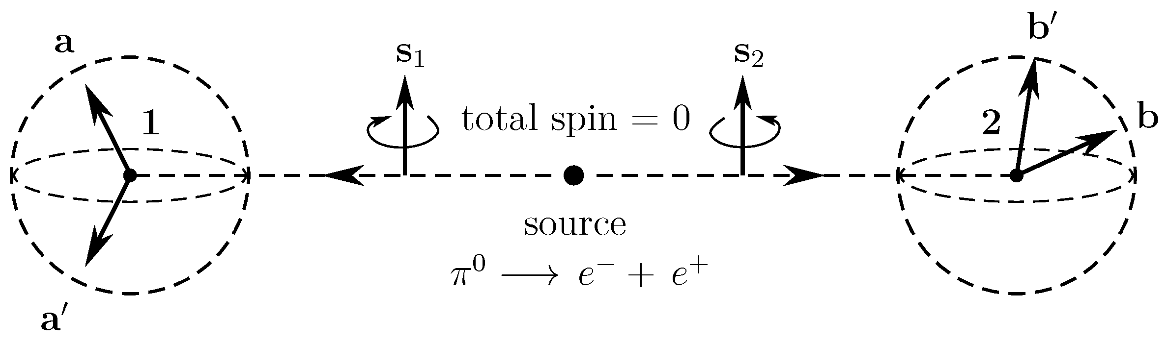
Now, the proof of Bell’s famous theorem [1] is based on Bohm’s spin version of the EPR’s thought experiment [24], which involves an entangled pair of spin-$\frac{1}{2}$ particles emerging from a source and moving freely in opposite directions, with particles 1 and 2 subject, respectively, to spin measurements along independently chosen unit directions $\mathbf{a}$ and $\mathbf{b}$ by Alice and Bob, who are stationed at a spacelike separated distance from each other (see Figure 1). If initially the pair has vanishing total spin, then quantum mechanical state of the system is described by the entangled singlet state

$$|\mathsf{\Psi }\rangle =\frac{1}{\sqrt{2}}\left\{{|\mathbf{k},+\rangle }_1{\otimes |\mathbf{k},-\rangle }_2{-|\mathbf{k},-\rangle }_1\otimes {|\mathbf{k},+\rangle }_2\right\},$$

(10)

where $\mathbf{k}$ is an arbitrary unit vector in $\mathrm{I}{\mathrm{R}}^3$ and

$$\sigma ·\mathbf{k}|\mathbf{k},\pm \rangle =\pm |\mathbf{k},\pm \rangle$$

(11)

defines quantum mechanical eigenstates in which the two fermions have spins “up” or “down” in the units of $\hslash =2$, with $\sigma$ being the Pauli spin “vector” $({\sigma }_x,{\sigma }_y,{\sigma }_z)$. Once the state (10) is prepared, the observable $\mathsf{\Omega }\left(c\right)$ of interest is

$$\mathsf{\Omega }\left(c\right)={\sigma }_1·\mathbf{a}\otimes {\sigma }_2·\mathbf{b},$$

(12)

whose possible eigenvalues are

$$\omega (c,\lambda )=\mathcal{A}\mathcal{B}(\mathbf{a},\mathbf{b},\lambda )=\pm 1,$$

(13)

where $\mathcal{A}=\pm 1$ and $\mathcal{B}=\pm 1$ are the results of spin measurements made jointly by Alice and Bob along their randomly chosen detector directions $\mathbf{a}$ and $\mathbf{b}$. In the singlet state (10) the joint observable (12) predicts sinusoidal correlations $\langle \mathsf{\Psi }|{\sigma }_1·\mathbf{a}\otimes {\sigma }_2·\mathbf{b}|\mathsf{\Psi }\rangle =-\mathbf{a}·\mathbf{b}$ between the values of the spins observed about the freely chosen contexts $\mathbf{a}$ and $\mathbf{b}$ [5].

For locally contextual hidden variable theories there is a further requirement that the results of local measurements must be describable by functions that respect local causality, as first envisaged by Einstein [19] and later formulated mathematically by Bell [1]. It can be satisfied by requiring that the eigenvalue $\omega (c,\lambda )$ of the observable $\mathsf{\Omega }\left(c\right)$ in (12) representing the joint result $\mathcal{A}\mathcal{B}(\mathbf{a},\mathbf{b},\lambda )=\pm 1$ is factorizable as $\omega (c,\lambda )={\omega }_1(c_1,\lambda ){\omega }_2(c_2,\lambda )$, or in Bell’s notation as

$$\mathcal{A}\mathcal{B}(\mathbf{a},\mathbf{b},\lambda )=\mathcal{A}(\mathbf{a},\lambda )\mathcal{B}(\mathbf{b},\lambda ),$$

(14)

with the factorized functions $\mathcal{A}(\mathbf{a},\lambda )=\pm 1$ and $\mathcal{B}(\mathbf{b},\lambda )=\pm 1$ satisfying the following condition of local causality:

Apart from the hidden variables $\lambda$, the result $\mathcal{A}=\pm 1$ of Alice depends only on the measurement context $\mathbf{a}$, chosen freely by Alice, regardless of Bob’s actions. And, likewise, apart from the hidden variables $\lambda$, the result $\mathcal{B}=\pm 1$ of Bob depends only on the measurement context $\mathbf{b}$, chosen freely by Bob, regardless of Alice’s actions. In particular, the function $\mathcal{A}(\mathbf{a},\lambda )$does not depend on $\mathbf{b}$ or $\mathcal{B}$ and the function $\mathcal{B}(\mathbf{b},\lambda )$does not depend on $\mathbf{a}$ or $\mathcal{A}$. Moreover, the hidden variables $\lambda$ do not depend on either $\mathbf{a}$, $\mathbf{b}$, $\mathcal{A}$, or $\mathcal{B}$ [10].

The expectation value $\mathcal{E}(\mathbf{a},\mathbf{b})$ of the joint results in the dispersion-free state $|\psi ,\lambda )$ should then satisfy the condition

$$\langle \mathsf{\Psi }|{\sigma }_1·\mathbf{a}\otimes {\sigma }_2·\mathbf{b}|\mathsf{\Psi }\rangle =\mathcal{E}(\mathbf{a},\mathbf{b}):={\int }_{\mathcal{L}}\mathcal{A}(\mathbf{a},\lambda )\mathcal{B}(\mathbf{b},\lambda )p\left(\lambda \right)d\lambda ,$$

(15)

where the hidden variables $\lambda$ originate from a source located in the overlap of the backward light-cones of Alice and Bob, and the normalized probability distribution $p\left(\lambda \right)$ is assumed to remain statistically independent of the contexts $\mathbf{a}$ and $\mathbf{b}$ so that $p\left(\lambda \right|\mathbf{a},\mathbf{b})=p(\lambda )$, which is a reasonable assumption. In fact, relaxing this assumption to allow $p\left(\lambda \right)$ to depend on $\mathbf{a}$ and $\mathbf{b}$ introduces a form of non-locality, as explained by Clauser and Horne in footnote 13 of [25]. Then, since $\mathcal{A}(\mathbf{a},\lambda )=\pm 1$ and $\mathcal{B}(\mathbf{b},\lambda )=\pm 1$, their product $\mathcal{A}(\mathbf{a},\lambda )\mathcal{B}(\mathbf{b},\lambda )=\pm 1$, setting the following bounds on $\mathcal{E}(\mathbf{a},\mathbf{b})$:

$$-1⩽\mathcal{E}(\mathbf{a},\mathbf{b})⩽+1.$$

(16)

These bounds are respected not only by local hidden variable theories but also by quantum mechanics and experiments.

IV. Mathematical Core of Bell’s Theorem

By contrast, at the heart of Bell’s theorem is a derivation of the bounds of $\pm 2$ on a combination of the expectation values $\mathcal{E}(\mathbf{a},\mathbf{b})$ of local results $\mathcal{A}(\mathbf{a},\lambda )$ and $\mathcal{B}(\mathbf{b},\lambda )$, recorded at remote observation stations by Alice and Bob, from four different sub-experiments involving measurements of non-commuting observables such as ${\sigma }_1·\mathbf{a}$ and ${\sigma }_1·{\mathbf{a}}^{\prime }$ [1,16]:

$$\mathcal{E}(\mathbf{a},\mathbf{b})+\mathcal{E}(\mathbf{a},{\mathbf{b}}^{\prime })+\mathcal{E}({\mathbf{a}}^{\prime },\mathbf{b})-\mathcal{E}({\mathbf{a}}^{\prime },{\mathbf{b}}^{\prime }).$$

(17)

Alice can freely choose a detector direction $\mathbf{a}$ or ${\mathbf{a}}^{\prime }$, and likewise Bob can freely choose a detector direction $\mathbf{b}$ or ${\mathbf{b}}^{\prime }$, to detect, at a space-like distance from each other, the spins of fermions they receive from the common source. Then, from (16), we can immediately read off the upper and lower bounds on the combination (17) of expectation values:

$$-4⩽\mathcal{E}(\mathbf{a},\mathbf{b})+\mathcal{E}(\mathbf{a},{\mathbf{b}}^{\prime })+\mathcal{E}({\mathbf{a}}^{\prime },\mathbf{b})-\mathcal{E}({\mathbf{a}}^{\prime },{\mathbf{b}}^{\prime })⩽+4.$$

(18)

The next step in Bell’s derivation of the bounds $\pm 2$ instead of $\pm 4$ is the assumption of additivity of expectation values:

$$\begin{array}{cc}\hfill & \mathcal{E}(\mathbf{a},\mathbf{b})+\mathcal{E}(\mathbf{a},{\mathbf{b}}^{\prime })+\mathcal{E}({\mathbf{a}}^{\prime },\mathbf{b})-\mathcal{E}({\mathbf{a}}^{\prime },{\mathbf{b}}^{\prime })\hfill \\ \hfill & ={\int }_{\mathcal{L}}\mathcal{A}(\mathbf{a},\lambda )\mathcal{B}(\mathbf{b},\lambda )p\left(\lambda \right)d\lambda +{\int }_{\mathcal{L}}\mathcal{A}(\mathbf{a},\lambda )\mathcal{B}({\mathbf{b}}^{\prime },\lambda )p\left(\lambda \right)d\lambda +{\int }_{\mathcal{L}}\mathcal{A}({\mathbf{a}}^{\prime },\lambda )\mathcal{B}(\mathbf{b},\lambda )p\left(\lambda \right)d\lambda \hfill \\ \hfill & -{\int }_{\mathcal{L}}\mathcal{A}({\mathbf{a}}^{\prime },\lambda )\mathcal{B}({\mathbf{b}}^{\prime },\lambda )p\left(\lambda \right)d\lambda \hfill \\ \hfill & ={\int }_{\mathcal{L}}\left\{\mathcal{A}(\mathbf{a},\lambda )\mathcal{B}(\mathbf{b},\lambda )+\mathcal{A}(\mathbf{a},\lambda )\mathcal{B}({\mathbf{b}}^{\prime },\lambda )+\mathcal{A}({\mathbf{a}}^{\prime },\lambda )\mathcal{B}(\mathbf{b},\lambda )-\mathcal{A}({\mathbf{a}}^{\prime },\lambda )\mathcal{B}({\mathbf{b}}^{\prime },\lambda )\right\}p\left(\lambda \right)d\lambda .\hfill \end{array}$$

(19)

We will have much to discuss about this step, but if we accept the last equality, then the bounds of $\pm 2$ on Bell-CHSH combination (17) of expectation values is not difficult to work out by rewriting the integrand on its right-hand side as

$$\mathcal{A}(\mathbf{a},\lambda )\left\{\mathcal{B}(\mathbf{b},\lambda )+\mathcal{B}({\mathbf{b}}^{\prime },\lambda )\right\}+\mathcal{A}({\mathbf{a}}^{\prime },\lambda )\left\{\mathcal{B}(\mathbf{b},\lambda )-\mathcal{B}({\mathbf{b}}^{\prime },\lambda )\right\}.$$

(20)

Since $\mathcal{B}(\mathbf{b},\lambda )=\pm 1$, if $|\mathcal{B}(\mathbf{b},\lambda )+\mathcal{B}({\mathbf{b}}^{\prime },\lambda )|=2$, then $|\mathcal{B}(\mathbf{b},\lambda )-\mathcal{B}({\mathbf{b}}^{\prime },\lambda )|=0$, and vice versa. Consequently, since $\mathcal{A}(\mathbf{a},\lambda )=\pm 1$, the integrand (20) is bounded by $\pm 2$ and the absolute value of the last integral in (19) does not exceed2:

$$\begin{array}{c}-2⩽{\int }_{\mathcal{L}}\{\mathcal{A}(\mathbf{a},\lambda )\mathcal{B}(\mathbf{b},\lambda )+\mathcal{A}(\mathbf{a},\lambda )\mathcal{B}({\mathbf{b}}^{\prime },\lambda )+\mathcal{A}({\mathbf{a}}^{\prime },\lambda )\mathcal{B}(\mathbf{b},\lambda )\\ -\mathcal{A}({\mathbf{a}}^{\prime },\lambda )\mathcal{B}({\mathbf{b}}^{\prime },\lambda )\}p\left(\lambda \right)d\lambda ⩽+2.\end{array}$$

(21)

Therefore, the equality (19) implies that the absolute value of the combination of expectation values is bounded by 2:

$$-2⩽\mathcal{E}(\mathbf{a},\mathbf{b})+\mathcal{E}(\mathbf{a},{\mathbf{b}}^{\prime })+\mathcal{E}({\mathbf{a}}^{\prime },\mathbf{b})-\mathcal{E}({\mathbf{a}}^{\prime },{\mathbf{b}}^{\prime })⩽+2.$$

(22)

But since the bounds on (17) predicted by quantum mechanics and observed in experiments are $\pm 2\sqrt{2}$, Bell concludes that no local and realistic theory envisaged by Einstein can reproduce the statistical predictions of quantum mechanics. In particular, contextual hidden variable theories specified by (7) that respect the factorizability (14) are not viable.

Now, it is not difficult to demonstrate the converse of the above derivation in which the additivity of expectation values (19) is derived by assuming the stringent bounds of $\pm 2$ on the sum (17). Employing (15), (17) can be writtenas

$$\begin{array}{c}{\int }_{\mathcal{L}}\mathcal{A}(\mathbf{a},\lambda )\mathcal{B}(\mathbf{b},\lambda )p\left(\lambda \right)d\lambda +{\int }_{\mathcal{L}}\mathcal{A}(\mathbf{a},\lambda )\mathcal{B}({\mathbf{b}}^{\prime },\lambda )p\left(\lambda \right)d\lambda +{\int }_{\mathcal{L}}\mathcal{A}({\mathbf{a}}^{\prime },\lambda )\mathcal{B}(\mathbf{b},\lambda )p\left(\lambda \right)d\lambda \\ -{\int }_{\mathcal{L}}\mathcal{A}({\mathbf{a}}^{\prime },\lambda )\mathcal{B}({\mathbf{b}}^{\prime },\lambda )p\left(\lambda \right)d\lambda .\end{array}$$

(23)

Since each product $\mathcal{A}(\mathbf{a},\lambda )\mathcal{B}(\mathbf{b},\lambda )$ in the above integrals is equal to $\pm 1$, each of the four integrals is bounded by $\pm 1$:

$$-1⩽{\int }_{\mathcal{L}}\mathcal{A}(\mathbf{a},\lambda )\mathcal{B}(\mathbf{b},\lambda )p\left(\lambda \right)d\lambda ⩽+1.$$

(24)

Thus the sum of four integrals in (23) is bounded by $\pm 4$, not $\pm 2$. However, we started with (22), which contends that the sum of integrals in (23) is bounded by $\pm 2$. But the only way to reduce the bounds on (23) from $\pm 4$ to $\pm 2$ without violating the rules of anti-derivatives is by equating the sum of integrals in (23) to the following integral of the sum,

$${\int }_{\mathcal{L}}\left\{\mathcal{A}(\mathbf{a},\lambda )\mathcal{B}(\mathbf{b},\lambda )+\mathcal{A}(\mathbf{a},\lambda )\mathcal{B}({\mathbf{b}}^{\prime },\lambda )+\mathcal{A}({\mathbf{a}}^{\prime },\lambda )\mathcal{B}(\mathbf{b},\lambda )-\mathcal{A}({\mathbf{a}}^{\prime },\lambda )\mathcal{B}({\mathbf{b}}^{\prime },\lambda )\right\}p\left(\lambda \right)d\lambda ,$$

(25)

which, as we saw above in (21), is bounded by $\pm 2$. We have thus derived the additivity of expectation values (19) by imposing (22) as our starting assumption. Thus, given the previous derivation that led us to (22) by assuming (19) and the current derivation that led us to (19) by assuming (22), we have proved that the assumption (19) of the additivity of expectation values is tautologous to assuming the bounds of $\pm 2$ on Bell-CHSH combination (17) of expectation values.

In many derivations of (22) in the literature, factorized probabilities of observing binary measurement results are employed rather than measurement results themselves I have used in (14) in my derivation following Bell [1,16]. But employing probabilities would only manage to obfuscate the logical flaw in Bell’s argument I intend to bring out here.

V. Additivity of Expectation Values Is Respected by Quantum States

The key step that led us to the bounds of $\pm 2$ on (17) that are more restrictive than $\pm 2\sqrt{2}$ is the assumption (19) of additivity of expectation values. This assumption, however, is usually not viewed as an assumption at all. It is usually viewed as a benign mathematical step, necessitated by Einstein’s requirement of realism. But as I will demonstrate in Section VI, far from being required by realism, the right-hand side of (19), in fact, contradicts that requirement.

Moreover, realism has already been adequately accommodated by the very definition of the local functions $\mathcal{A}(\mathbf{a},\lambda )$ and $\mathcal{B}(\mathbf{b},\lambda )$ and their counterfactual juxtaposition on the left-hand side of (19), as contextually existing properties of the system. Evidently, while a result in only one of the four expectation values corresponding to a sub-experiment that appear on the left-hand side of (19) can be realized in a given run of a Bell-test experiment, the remaining three results appearing on that side are realizable at least counterfactually, thus fulfilling the requirement of realism [8]. Therefore, the requirement of realism does not necessitate the left-hand side of (19) to be equated with its right-hand side in the derivation of (22). Realism requires definite results $\mathcal{A}(\mathbf{a},\lambda )\mathcal{B}(\mathbf{b},\lambda )$ to exist as eigenvalues only counterfactually, not all four at once, as they are written on the right-hand side of (19). What is more, as we will soon see, realism implicit in the prescription (7) requires the quantity (20) to be a correct eigenvalue of the summed operator (33), but it is not.

On the other hand, given the assumption $p\left(\lambda \right|\mathbf{a},\mathbf{b})=p(\lambda )$ of statistical independence and the addition property of anti-derivatives, mathematically the equality (19) follows at once. The binary properties of the functions $\mathcal{A}(\mathbf{a},\lambda )$ and $\mathcal{B}(\mathbf{b},\lambda )$ then immediately leads to the bounds of $\pm 2$ on the Bell-CHSH sum (17). But, as we saw above, assuming the bounds of $\pm 2$ on (17) leads, conversely, to the assumption (19) of the additivity of expectation values. Thus, assuming the additivity of expectation values (19) is mathematically equivalent to assuming the bounds of $\pm 2$ on the sum (17). In other words, Bell’s argument presented in Section IV assumes its conclusion (22) in the guise of assumption (19).

Sometimes assumption (19) is justified on statistical grounds. It is argued that the four sub-experiments appearing on the left-hand side of (19) with different experimental settings $\{\mathbf{a},\mathbf{b}\}$, $\{\mathbf{a},{\mathbf{b}}^{\prime }\}$, etc. can be performed independently of each other, on possibly different occasions, and then the resulting averages are added together at a later time for statistical analysis. If the number of experimental runs for each pair of settings is sufficiently large, then, theoretically, the sum of the four averages appearing on the left-hand side of (19) are found not to exceed the bounds of $\pm 2$, thus justifying the equality (19). This can be easily verified in numerical simulations [4]. But what this statistical argument neglects to take into account is that the four sub-experiments in question involve mutually exclusive pairs of settings such as $\{\mathbf{a},\mathbf{b}\}$ and $\{\mathbf{a},{\mathbf{b}}^{\prime }\}$, and thus involve non-commuting observables that cannot be measured simultaneously. Unless the statistical analysis takes this physical fact into account, such an argument amounts to implicitly assuming that the four spin observables ${\sigma }_1·\mathbf{a}\otimes {\sigma }_2·\mathbf{b}$, etc. are mutually commuting, and thus simultaneously measurable, for which assumption (19) is valid. In other words, such an argument is simply assumption (19) in a statistical disguise.

Another important point to recognize here is that the above derivation of the stringent bounds of $\pm 2$ on (17) for a locally causal dispersion-free counterpart $|\psi ,\lambda )$ of the quantum mechanical singlet state (10) must comply with the heuristics of the contextual hidden variable theories we discussed in Section II. If it does not, then the bounds of $\pm 2$ cannot be claimed to have any relevance for the viability of local hidden variable theories [23]. Therefore, as discussed in Section II, in a contextual hidden variable theory all of the observables ${\mathsf{\Omega }}_i\left(c_i\right)$ of any physical system, including their sum $\tilde{\mathsf{\Omega }}\left(\tilde{c}\right)={\sum }_{i=1}^n{\mathsf{\Omega }}_i\left(c_i\right)$ (which also represents a physical quantity in the Hilbert space formulation of quantum mechanics [2] whether or not it is observed), must be assigned unique eigenvalues ${\omega }_i(c_i,\lambda )$ and $\tilde{\omega }(\tilde{c},\lambda )$, respectively, in the dispersion-free states $|\psi ,\lambda )$ of the system, regardless of whether these observables are simultaneously measurable.

Now, within quantum mechanics, expectation values do add in analogy with the equality (19) assumed by Bell for local hidden variable theories [2,17]. In quantum mechanics, the statistical predictions of which any hidden variable theory is obliged to reproduce, the joint results $\mathcal{A}(\mathbf{a},\lambda )\mathcal{B}(\mathbf{b},\lambda )$ observed by Alice and Bob would be eigenvalues of the operators ${\sigma }_1·\mathbf{a}\otimes {\sigma }_2·\mathbf{b}$, and the linearity in the rules of Hilbert space quantum mechanics ensures that these operators satisfy the additivity of expectation values. Thus, for any quantum state $|\psi \rangle$, the following equality holds:

$$\begin{array}{cc}\hfill \langle \psi |{\sigma }_1·\mathbf{a}& \otimes {\sigma }_2·\mathbf{b}|\psi \rangle +\langle \psi |{\sigma }_1·\mathbf{a}\otimes {\sigma }_2·{\mathbf{b}}^{\prime }|\psi \rangle +\langle \psi |{\sigma }_1·{\mathbf{a}}^{\prime }\otimes {\sigma }_2·\mathbf{b}|\psi \rangle -\langle \psi |{\sigma }_1·{\mathbf{a}}^{\prime }\otimes {\sigma }_2·{\mathbf{b}}^{\prime }|\psi \rangle \hfill \\ \hfill & =\langle \psi |{\sigma }_1·\mathbf{a}\otimes {\sigma }_2·\mathbf{b}+{\sigma }_1·\mathbf{a}\otimes {\sigma }_2·{\mathbf{b}}^{\prime }+{\sigma }_1·{\mathbf{a}}^{\prime }\otimes {\sigma }_2·\mathbf{b}-{\sigma }_1·{\mathbf{a}}^{\prime }\otimes {\sigma }_2·{\mathbf{b}}^{\prime }|\psi \rangle .\hfill \end{array}$$

(26)

Comparing (19) and (A1), the equality between the two sides of (19) seems reasonable, even physically. Furthermore, since the condition (15) for any hidden variable theory obliges us to set the four terms on the left-hand side of (A1) as

$$\begin{array}{cc}\hfill \langle \mathsf{\Psi }|{\sigma }_1·\mathbf{a}\otimes {\sigma }_2·\mathbf{b}|\mathsf{\Psi }\rangle & ={\int }_{\mathcal{L}}\mathcal{A}(\mathbf{a},\lambda )\mathcal{B}(\mathbf{b},\lambda )p\left(\lambda \right)d\lambda ,\hfill \end{array}$$

(27)

$$\begin{array}{cc}\hfill \langle \mathsf{\Psi }|{\sigma }_1·\mathbf{a}\otimes {\sigma }_2·{\mathbf{b}}^{\prime }|\mathsf{\Psi }\rangle & ={\int }_{\mathcal{L}}\mathcal{A}(\mathbf{a},\lambda )\mathcal{B}({\mathbf{b}}^{\prime },\lambda )p\left(\lambda \right)d\lambda ,\hfill \end{array}$$

(28)

$$\begin{array}{cc}\hfill \langle \mathsf{\Psi }|{\sigma }_1·{\mathbf{a}}^{\prime }\otimes {\sigma }_2·\mathbf{b}|\mathsf{\Psi }\rangle & ={\int }_{\mathcal{L}}\mathcal{A}({\mathbf{a}}^{\prime },\lambda )\mathcal{B}(\mathbf{b},\lambda )p\left(\lambda \right)d\lambda ,\hfill \end{array}$$

(29)

$$\begin{array}{cc}\hfill \mathrm{and}\langle \mathsf{\Psi }|{\sigma }_1·{\mathbf{a}}^{\prime }\otimes {\sigma }_2·{\mathbf{b}}^{\prime }|\mathsf{\Psi }\rangle & ={\int }_{\mathcal{L}}\mathcal{A}({\mathbf{a}}^{\prime },\lambda )\mathcal{B}({\mathbf{b}}^{\prime },\lambda )p\left(\lambda \right)d\lambda ,\hfill \end{array}$$

(30)

it may seem reasonable that, given the quantum mechanical equality (A1), any hidden variable theory should satisfy

$$\begin{array}{cc}\hfill \langle \mathsf{\Psi }\left|\tilde{\mathsf{\Omega }}\left(\tilde{c}\right)\right|\mathsf{\Psi }\rangle & =\langle \mathsf{\Psi }|{\sigma }_1·\mathbf{a}\otimes {\sigma }_2·\mathbf{b}+{\sigma }_1·\mathbf{a}\otimes {\sigma }_2·{\mathbf{b}}^{\prime }+{\sigma }_1·{\mathbf{a}}^{\prime }\otimes {\sigma }_2·\mathbf{b}-{\sigma }_1·{\mathbf{a}}^{\prime }\otimes {\sigma }_2·{\mathbf{b}}^{\prime }|\mathsf{\Psi }\rangle \hfill \\ \hfill & ={\int }_{\mathcal{L}}\{\mathcal{A}(\mathbf{a},\lambda )\mathcal{B}(\mathbf{b},\lambda )+\mathcal{A}(\mathbf{a},\lambda )\mathcal{B}({\mathbf{b}}^{\prime },\lambda )+\mathcal{A}({\mathbf{a}}^{\prime },\lambda )\mathcal{B}(\mathbf{b},\lambda )\hfill \\ \hfill & -\mathcal{A}({\mathbf{a}}^{\prime },\lambda )\mathcal{B}({\mathbf{b}}^{\prime },\lambda )\}p\left(\lambda \right)d\lambda ,\hfill \end{array}$$

(31)

adhering to the prescription (7), which would then justify equality (19). Since hidden variable theories are required to satisfy the prescription (7), should not they also reproduce equation (A6)? The answer to this is not straightforward.

VI. Additivity of Expectation Values Does Not Hold for Dispersion-Free States

The problem with equation (A6) is that, while the joint results $\mathcal{A}(\mathbf{a},\lambda )\mathcal{B}(\mathbf{b},\lambda )$, etc. appearing on the left-hand side of equation (19) are possible eigenvalues of the products of spin operators ${\sigma }_1·\mathbf{a}\otimes {\sigma }_2·\mathbf{b}$, etc., their summation

$$\mathcal{A}(\mathbf{a},\lambda )\mathcal{B}(\mathbf{b},\lambda )+\mathcal{A}(\mathbf{a},\lambda )\mathcal{B}({\mathbf{b}}^{\prime },\lambda )+\mathcal{A}({\mathbf{a}}^{\prime },\lambda )\mathcal{B}(\mathbf{b},\lambda )-\mathcal{A}({\mathbf{a}}^{\prime },\lambda )\mathcal{B}({\mathbf{b}}^{\prime },\lambda )$$

(32)

appearing as the integrand on the right-hand side of equation (A6) or (19) is not an eigenvalue of the summed operator

$$\tilde{\mathsf{\Omega }}\left(\tilde{c}\right)={\sigma }_1·\mathbf{a}\otimes {\sigma }_2·\mathbf{b}+{\sigma }_1·\mathbf{a}\otimes {\sigma }_2·{\mathbf{b}}^{\prime }+{\sigma }_1·{\mathbf{a}}^{\prime }\otimes {\sigma }_2·\mathbf{b}-{\sigma }_1·{\mathbf{a}}^{\prime }\otimes {\sigma }_2·{\mathbf{b}}^{\prime },$$

(33)

because the spin operators ${\sigma }_1·\mathbf{a}$ and ${\sigma }_1·{\mathbf{a}}^{\prime }$, etc., and therefore ${\sigma }_1·\mathbf{a}\otimes {\sigma }_2·\mathbf{b}$, etc., do not commute with each other:

$$\begin{array}{cc}\hfill \left[{\sigma }_1·\mathbf{a}\otimes {\sigma }_2·\mathbf{b},{\sigma }_1·\mathbf{a}\otimes {\sigma }_2·{\mathbf{b}}^{\prime }\right]& =2\sigma ·\left\{\left(\mathbf{a}\times {\mathbf{b}}^{\prime }\right)\times \left(\mathbf{a}\times \mathbf{b}\right)\right\}\hfill \\ \hfill & \ne 0\mathrm{if}{\mathbf{b}}^{\prime }\ne \mathbf{b}\ne \mathbf{a}.\hfill \end{array}$$

(34)

Consequently, equation (A6) would hold within any hidden variable theory only if the operators ${\sigma }_1·\mathbf{a}\otimes {\sigma }_2·\mathbf{b}$, etc. were commuting operators. This is well known from the famous criticisms of von Neumann’s theorem against hidden variable theories (see, e.g.,8] and references therein). While the equality (19) of the sum of expectation values with the expectation value of the sum is respected in quantum mechanics, it does not hold for hidden variable theories [17].

In [17], Bell illustrates this problem using spin components of a spin-$\frac{1}{2}$ particle. Suppose we make a measurement of the component ${\sigma }_x$ of the spin with a Stern-Gerlach magnet suitably oriented in $\mathrm{I}{\mathrm{R}}^3$. That would yield an eigenvalue $s_x$ of ${\sigma }_x$ as a result. However, if we wish to measure the component ${\sigma }_y$ of the spin, then that would require a different orientation of the magnet in $\mathrm{I}{\mathrm{R}}^3$, and would give a different eigenvalue, $s_y$ of ${\sigma }_y$, as a result. Moreover, a measurement of the sum of the x- and y-components of the spin, ${\sigma }_x+{\sigma }_y$, would again require a very different orientation of the magnet in $\mathrm{I}{\mathrm{R}}^3$. Therefore, the result obtained as an eigenvalue of the summed operators ${\sigma }_x+{\sigma }_y$ will not be the sum $s_x+s_y$ of an eigenvalue of the operator ${\sigma }_x$ added linearly to an eigenvalue of the operator ${\sigma }_y$. As Bell points out in [17], the additivity of expectation values $\langle \psi |{\sigma }_x|\psi \rangle +\langle \psi |{\sigma }_y|\psi \rangle =\langle \psi |{\sigma }_x+{\sigma }_y|\psi \rangle$ is a rather unusual property of the quantum states $|\psi \rangle$. It does not hold for the dispersion-free states $|\psi ,\lambda )$ of hidden variable theories because the eigenvalues of non-commuting observables such as ${\sigma }_x$ and ${\sigma }_y$ do not add linearly, as we noted at the end of Section II. Consequently, the additivity relation (19) that holds for quantum states would not hold for the dispersion-free states.

This problem, however, suggests its own resolution. We can work out the correct eigenvalue $\tilde{\omega }(\tilde{c},\lambda )$ of the summed operator (33), at least formally, as I have worked out in Appendix A below. The correct version of equation (A6) is then

$$\langle \mathsf{\Psi }|{\sigma }_1·\mathbf{a}\otimes {\sigma }_2·\mathbf{b}+{\sigma }_1·\mathbf{a}\otimes {\sigma }_2·{\mathbf{b}}^{\prime }+{\sigma }_1·{\mathbf{a}}^{\prime }\otimes {\sigma }_2·\mathbf{b}-{\sigma }_1·{\mathbf{a}}^{\prime }\otimes {\sigma }_2·{\mathbf{b}}^{\prime }|\mathsf{\Psi }\rangle ={\int }_{\mathcal{L}}\tilde{\omega }(\mathbf{a},{\mathbf{a}}^{\prime },\mathbf{b},{\mathbf{b}}^{\prime },\lambda )p\left(\lambda \right)d\lambda ,$$

(35)

where

$$\tilde{\omega }=\pm \sqrt{{\left\{\mathcal{A}(\mathbf{a},\lambda )\mathcal{B}(\mathbf{b},\lambda )+\mathcal{A}(\mathbf{a},\lambda )\mathcal{B}({\mathbf{b}}^{\prime },\lambda )+\mathcal{A}({\mathbf{a}}^{\prime },\lambda )\mathcal{B}(\mathbf{b},\lambda )-\mathcal{A}({\mathbf{a}}^{\prime },\lambda )\mathcal{B}({\mathbf{b}}^{\prime },\lambda )\right\}}^2+(\mathsf{\Psi },\lambda |\tilde{\mathsf{\Theta }}|\mathsf{\Psi },\lambda )\ne 0}$$

(36)

is the correct eigenvalue of the summed operator (33), with its non-commuting part separated out as the operator

$$\tilde{\mathsf{\Theta }}(\mathbf{a},{\mathbf{a}}^{\prime },\mathbf{b},{\mathbf{b}}^{\prime })=2\sigma ·\mathbf{n}(\mathbf{a},{\mathbf{a}}^{\prime },\mathbf{b},{\mathbf{b}}^{\prime }),$$

(37)

where

$$\begin{array}{cc}\hfill \mathbf{n}(\mathbf{a},{\mathbf{a}}^{\prime },\mathbf{b},{\mathbf{b}}^{\prime })=\{\left(\mathbf{a}\times {\mathbf{b}}^{\prime }\right)\times \left(\mathbf{a}\times \mathbf{b}\right)& +\left({\mathbf{a}}^{\prime }\times \mathbf{b}\right)\times \left(\mathbf{a}\times \mathbf{b}\right)+\left({\mathbf{a}}^{\prime }\times \mathbf{b}\right)\times \left(\mathbf{a}\times {\mathbf{b}}^{\prime }\right)\hfill \\ \hfill & -\left({\mathbf{a}}^{\prime }\times {\mathbf{b}}^{\prime }\right)\times \left(\mathbf{a}\times \mathbf{b}\right)-\left({\mathbf{a}}^{\prime }\times {\mathbf{b}}^{\prime }\right)\times \left({\mathbf{a}}^{\prime }\times \mathbf{b}\right)\hfill \\ \hfill & -\left({\mathbf{a}}^{\prime }\times {\mathbf{b}}^{\prime }\right)\times \left(\mathbf{a}\times {\mathbf{b}}^{\prime }\right)\}.\hfill \end{array}$$

(38)

The details of how this separation is accomplished using (34) can be found in Appendix A below. From (36), it is now easy to appreciate that the additivity of expectation values (19) assumed by Bell can hold only if the expectation value $(\mathsf{\Psi },\lambda |\tilde{\mathsf{\Theta }}|\mathsf{\Psi },\lambda )=\pm 2\left|\right|\mathbf{n}\left|\right|$ of the non-commuting part within the eigenvalue $\tilde{\omega }(\mathbf{a},{\mathbf{a}}^{\prime },\mathbf{b},{\mathbf{b}}^{\prime },\lambda )$ of the summed operator (33) is zero. But that is possible only if the operators ${\sigma }_1·\mathbf{a}\otimes {\sigma }_2·\mathbf{b}$, etc. constituting the sum (33) commute with each other. In general, if the operators ${\sigma }_1·\mathbf{a}\otimes {\sigma }_2·\mathbf{b}$, etc. in (33) do not commute with each other, then we would have

$$\tilde{\omega }(\mathbf{a},{\mathbf{a}}^{\prime },\mathbf{b},{\mathbf{b}}^{\prime },\lambda )\ne \mathcal{A}(\mathbf{a},\lambda )\mathcal{B}(\mathbf{b},\lambda )+\mathcal{A}(\mathbf{a},\lambda )\mathcal{B}({\mathbf{b}}^{\prime },\lambda )+\mathcal{A}({\mathbf{a}}^{\prime },\lambda )\mathcal{B}(\mathbf{b},\lambda )-\mathcal{A}({\mathbf{a}}^{\prime },\lambda )\mathcal{B}({\mathbf{b}}^{\prime },\lambda ).$$

(39)

But the operators ${\sigma }_1·\mathbf{a}\otimes {\sigma }_2·\mathbf{b}$, etc. indeed do not commute with each other, because the pairs of directions $\{\mathbf{a},{\mathbf{a}}^{\prime }\}$, etc. in (33) are mutually exclusive directions in $\mathrm{I}{\mathrm{R}}^3$. Therefore, the additivity of expectation values assumed at step (19) in the derivation of (22) is unjustifiable. Far from being necessitated by realism, it actually contradicts realism.

Since three of the four results appearing in the sum (32) can exist only counterfactually, the sum in (32) cannot exist even counterfactually. Thus, in addition to not being a correct eigenvalue of the summed operator (33) as required by the prescription (7) for any contextual hidden variable theories, the quantity appearing in (32) is, in fact, an entirely fictitious quantity, with no counterpart in any possible world, apart from in the trivial case when all observables are commutative. By contrast, the correct eigenvalue (36) of the summed operator (33) can exist at least counterfactually because it is a genuine eigenvalue of that quantum mechanical operator, thereby satisfying the requirement of realism correctly, in accordance with the prescription (7) for the hidden variable theories. Using (36), all five of the observables appearing on both sides of the quantum mechanical equation (A1) can be assigned unique and correct eigenvalues [8].

Once this oversight is ameliorated, it is not difficult to show that the conclusion of Bell’s theorem no longer follows. For then, using the correct eigenvalue (36) of (33) instead of (32) on the right-hand side of (19), we have the equation

$$\mathcal{E}(\mathbf{a},\mathbf{b})+\mathcal{E}(\mathbf{a},{\mathbf{b}}^{\prime })+\mathcal{E}({\mathbf{a}}^{\prime },\mathbf{b})-\mathcal{E}({\mathbf{a}}^{\prime },{\mathbf{b}}^{\prime })={\int }_{\mathcal{L}}\tilde{\omega }(\mathbf{a},{\mathbf{a}}^{\prime },\mathbf{b},{\mathbf{b}}^{\prime },\lambda )p\left(\lambda \right)d\lambda$$

(40)

instead of (19), which implements realism correctly on both of its sides, as required by the prescription (7) we discussed in Section II. This equation (40) is thus the correct dispersion-free counterpart of the equivalence (A1) for the quantum mechanical expectation values. It expresses the correct relationship among the expectation values for the singlet state in the local hidden variable framework considered by Bell [1]. Recall again from the end of Section II that the quantum mechanical relation (A1) is an unusual property of the quantum states $|\psi \rangle$. As Bell stressed in [17], “[t]here is no reason to demand it individually of the hypothetical dispersion free states, whose function it is to reproduce the measurable peculiarities of quantum mechanics when averaged over.” Moreover, in Section V of [8] I have demonstrated that the bounds on the right-hand side of (40) are $\pm 2\sqrt{2}$ instead of $\pm 2$. An alternative derivation of these bounds follows from the magnitude $\left|\right|\mathbf{n}\left|\right|$ of the vector defined in (38), which, as proved in Appendix B below, is bounded by 2, and therefore the eigenvalue $\pm 2\left|\right|\mathbf{n}\left|\right|$ of the operator (37) obtained as its expectation value $(\mathsf{\Psi },\lambda |\tilde{\mathsf{\Theta }}|\mathsf{\Psi },\lambda )$ is bounded by $\pm 4$, giving

$$-4⩽(\mathsf{\Psi },\lambda |\tilde{\mathsf{\Theta }}(\mathbf{a},{\mathbf{a}}^{\prime },\mathbf{b},{\mathbf{b}}^{\prime })|\mathsf{\Psi },\lambda )⩽+4.$$

(41)

Substituting these into (36), together with the bounds of $\pm 2$ we worked out before on the commuting part (32), gives

$$-2\sqrt{2}⩽\tilde{\omega }(\mathbf{a},{\mathbf{a}}^{\prime },\mathbf{b},{\mathbf{b}}^{\prime },\lambda )⩽+2\sqrt{2}.$$

(42)

Consequently, we obtain the following Tsirel’son’s bounds in the dispersion-free state, on the right-hand side of (40):

$$-2\sqrt{2}⩽{\int }_{\mathcal{L}}\tilde{\omega }(\mathbf{a},{\mathbf{a}}^{\prime },\mathbf{b},{\mathbf{b}}^{\prime },\lambda )p\left(\lambda \right)d\lambda ⩽+2\sqrt{2}.$$

(43)

Given the correct relation (40) between expectation values instead of the flawed assumption (19), we thus arrive at

$$-2\sqrt{2}⩽\mathcal{E}(\mathbf{a},\mathbf{b})+\mathcal{E}(\mathbf{a},{\mathbf{b}}^{\prime })+\mathcal{E}({\mathbf{a}}^{\prime },\mathbf{b})-\mathcal{E}({\mathbf{a}}^{\prime },{\mathbf{b}}^{\prime })⩽+2\sqrt{2}.$$

(44)

Since the bounds of $\pm 2\sqrt{2}$ we have derived on the Bell-CHSH sum of expectation values are the same as those predicted by quantum mechanics and observed in the Bell-test experiments, the conclusion of Bell’s theorem is mitigated. What is ruled out by these experiments is not local realism but the assumption of the additivity of expectation values, which does not hold for non-commuting observables in dispersion-free states of any hidden variable theories to begin with.

VII. Conclusion: Bell’s Theorem Assumes Its Conclusion (Petitio Principii)

Let me reiterate the main points discussed above. Together, they demonstrate that Bell’s theorem begs the question.

(1) The first point is that the derivation in Section IV of the bounds of $\pm 2$ on (17) for the dispersion-free counterpart $|\psi ,\lambda )$ of the singlet state (10) must comply with the heuristics of the contextual hidden variable theories discussed in Section II. Otherwise, the stringent bounds of $\pm 2$ cannot be claimed to have any relevance for hidden variable theories. This requires compliance with the prescription (7) that equates the quantum mechanical expectation values with their hidden variable counterparts for all observables, including any sums of observables, pertaining to the singlet system.

(2) The most charitable view of the equality (19) is that it is an assumption, over and above those of locality, realism, and all other auxiliary assumptions required for deriving the inequalities (22), because it is valid only for commuting observables. Far from being required by realism, it contradicts realism, because it fails to assign the correct eigenvalue (36) to the summed observable (33) as its realistic counterpart, as required by the prescription (7). Realism requires that all observables, including their sums, must be assigned unique eigenvalues, regardless of whether they are observed.

(3) Expectation values in dispersion-free states of hidden variable theories do not add linearly for observables that are not simultaneously measurable. And yet, Bell assumed linear additivity (19) within a local hidden variable model. Conversely, in the light of the heuristics of contextual hidden variable theories we discussed in Section II, assuming (19) is equivalent to assuming that the spin observables ${\sigma }_1·\mathbf{a}\otimes {\sigma }_2·\mathbf{b}$, etc. commute with each other; but they do not.

(4) When the correct eigenvalue (36) is assigned to the summed operator (33) replacing the incorrect step (19), the bounds on Bell-CHSH sum (17) work out to be $\pm 2\sqrt{2}$ instead of $\pm 2$, thus mitigating the conclusion of Bell’s theorem.

(5) As we proved in Section IV, the assumption (19) of the additivity of expectation values is equivalent to assuming the strong bounds of $\pm 2$ on Bell-CHSH sum (17) of expectation values. In other words, (19) and (22) are tautologous.

The first four points above invalidate assumption (19), and thus inequalities (22) on physical grounds, and the last one demonstrates that Bell’s theorem assumes its conclusion in a different guise, and is thus invalid on logical grounds.

In this paper I have focused on a formal and logical critique of Bell’s theorem. Elsewhere [9,13,15], I have developed a comprehensive local-realistic framework for understanding quantum correlations in terms of the geometry of the spatial part of one of the well known solutions of Einstein’s field equations of general relativity — namely, that of a quaternionic 3-sphere — taken as a physical space within which we are confined to perform Bell-test experiments. This shows, constructively, that contextually local hidden variable theories are not ruled out by Bell-test experiments. Since, as we discussed in Section III, the formal proof of Bell’s theorem is based on the entangled singlet state (10), in [4,5,7,10,11,12,14] I have reproduced the correlations predicted by (10) as a special case within the local-realistic framework proposed in [9,13,15]. I especially recommend the calculations presented in [7] and [14], which also discuss a macroscopic experiment that would be able to falsify the 3-sphere hypothesis I have proposed in these publications.

References

- Bell JS. 1964 On the Einstein Podolsky Rosen paradox. Physics. 1, 195–200. [CrossRef]
- Von Neumann J. 1955 Mathematical Foundations of Quantum Mechanics. Princeton, NJ: Princeton University Press.
- Coleman S., Mandula J. 1967 All possible symmetries of the S matrix. Physical Review. 159, 1251–1256. [CrossRef]
- Christian J. 2019 Bell’s theorem versus local realism in a quaternionic model of physical space. IEEE Access. 7, 133388–133409. [CrossRef]
- Christian J. 2007 Disproof of Bell’s theorem by Clifford algebra valued local variables. [CrossRef]
- Christian J. 2014 Disproof of Bell’s Theorem: Illuminating the Illusion of Entanglement. Second Edition. Boca Raton, Florida: Brwonwalker Press.
- Christian J. 2015 Macroscopic observability of spinorial sign changes under 2π rotations. Int. J. Theor. Phys. 54, 20–46. [CrossRef]
- Christian J. 2017 Oversights in the respective theorems of von Neumann and Bell are homologous. [CrossRef]
- Christian J. 2018 Quantum correlations are weaved by the spinors of the Euclidean primitives. R. Soc. Open Sci. 5, 180526. [CrossRef]
- Christian J. 2020 Dr. Bertlmann’s socks in the quaternionic world of ambidextral reality. IEEE Access. 8, 191028–191048. [CrossRef]
- Christian J. 2021 Reply to “Comment on ‘Dr. Bertlmann’s socks in the quaternionic world of ambidextral reality.” IEEE Access. 9, 72161–72171. [CrossRef]
- Christian J. 2022 Reply to “Comment on ‘Bell’s theorem versus local realism in a quaternionic model of physical space.” IEEE Access. 10, 14429–14439. [CrossRef]
- Christian J. 2022 Local origins of quantum correlations rooted in geometric algebra. [CrossRef]
- Christian J. 2022 Symmetric derivation of the singlet correlations within a quaternionic 3-sphere. [CrossRef]
- Christian J. 2022 Response to ‘Comment on “Quantum correlations are weaved by the spinors of the Euclidean primitives.”’ R. Soc. Open Sci. 9, 220147. [CrossRef]
- Clauser JF., Shimony A. 1978 Bell’s theorem: Experimental tests and implications. Rep. Prog. Phys. 41, 1881–1927. [CrossRef]
- Bell JS. 1966 On the problem of hidden variables in quantum mechanics. Rev. Mod. Phys. 38, 447–452. [CrossRef]
- Gudder S. 1970 On hidden-variable theories. Journal of Mathematical Physics. 11, 431–436. [CrossRef]
- Einstein A. 1948 Quantum mechanics and reality. Dialectica. 2, 320–324. [CrossRef]
- Kochen S., Specker EP. 1967 The problem of hidden variables in quantum mechanics. J. Math. Mech. 17, 59–87. [CrossRef]
- Belinfante FJ. 1973 A Survey of Hidden-Variables Theories. New York, NY: Pergamon Press.
- Gleason AM. 1957 Measures on the closed subspaces of a Hilbert space. J. Math. Mech. 6, 885–893. [CrossRef]
- Shimony A. 1984 Contextual hidden variables theories and Bell’s inequalities. Brit. J. Phil. Sci. 35, 25–45. [CrossRef]
- Bohm D. 1951 Quantum Theory. Englewood Cliffs, NJ: Prentice-Hall. pp 614–623.
- Clauser JF., Horne MA. 1974 Experimental consequences of objective local theories. Phys. Rev. D. 10, 526–35. [CrossRef]
Figure 1.
In an EPR-Bohm-type experiment, a spin-less fermion – such as a neutral pion – is assumed to decay from a source into an electron-positron pair, as depicted. Then, measurements of the spin components of each separated fermion are performed at space-like separated observation stations and , obtaining binary results and along directions and . The conservation of spin momentum dictates that the total spin of the system remains zero during its free evolution. After Ref. [4].
Disclaimer/Publisher’s Note: The statements, opinions and data contained in all publications are solely those of the individual author(s) and contributor(s) and not of MDPI and/or the editor(s). MDPI and/or the editor(s) disclaim responsibility for any injury to people or property resulting from any ideas, methods, instructions or products referred to in the content. |
© 2023 by the authors. Licensee MDPI, Basel, Switzerland. This article is an open access article distributed under the terms and conditions of the Creative Commons Attribution (CC BY) license (http://creativecommons.org/licenses/by/4.0/).
Copyright: This open access article is published under a Creative Commons CC BY 4.0 license, which permit the free download, distribution, and reuse, provided that the author and preprint are cited in any reuse.