
Submitted:
22 February 2025
Posted:
24 February 2025
You are already at the latest version
Abstract
This review explores the advances, setbacks and future possibilities of directed acyclic graphs (DAGs) as conceptual and analytical tools in applied and theoretical epidemiology. DAGs are speculative, theoretical, or literal, diagrammatic representations of unknown, uncertain or known data generating mechanisms (and dataset generating processes) in which the causal relationships between variables are determined on the basis of two over-riding principles – ‘directionality’ and ‘acyclicity’. Amongst the many strengths of DAGs are their transparency, simplicity, flexibility, methodological utility and epistemological credibility. All of these strengths can help applied epidemiological studies better mitigate (and acknowledge) the impact of avoidable (and unavoidable) biases in causal inference analyses based on observational/non-experimental data. They can also strengthen the credibility and utility of theoretical studies that use DAGs to identify and explore hitherto hidden sources of analytical and inferential bias. Nonetheless, and despite their apparent simplicity, the application of DAGs has suffered a number of setbacks due to weaknesses in understanding, practice and reporting. These include a failure to include all conceivable unmeasured/unknown/latent covariates when developing and specifying DAGs; and weaknesses in the reporting of DAGs containing more than a handful of variables (nodes) and paths (arcs), and those where the intended application(s) and rationale(s) involved is necessary for appreciating, evaluating and exploiting any causal insights they might offer. We propose two additional principles to address these weaknesses, and identify a number of opportunities where DAGs might yet lead to further advances in: the critical appraisal and synthesis of observational studies; the portability of causality-enhanced prediction; the identification of novel sources of bias; and the application of DAG-dataset consistency assessment to resolve pervasive uncertainty in the temporal positioning of time-variant and -invariant covariates.
Keywords:
Directed Acyclic Graph
; DAG
; causal inference
; prediction
; bias
; epistemology
1. Introduction
The origins of directed acyclic graphs (DAGs) date back to the emergence of ‘graph theory’ in the early 1700s [1]. DAGs are literal, theoretical or speculative diagrammatic representations of causal paths between variables that are constructed, as their name suggests, on the basis of two over-riding principles – ‘directionality’ and ‘acyclicity’ – which require that:
Principle 1: “All causal paths are ‘directed’” – such that for any pair of (asynchronous) variables (e.g., x and y) between which a causal relationship is known, theorized or speculated to exist, only one (either x or y) can represent the cause; and only the other (either y or x) can be its consequence (hence either: x → y or y → x; but neither x – y nor x ↔ y).
Principle 2: “No direct cyclical paths or indirect cyclical pathways (comprising sequences of multiple consecutive paths) are permitted” – such that no consequence can be its own direct or indirect cause (hence ‘acyclic’ [2] – a property that is a definitive feature of DAGs and reflects what is known as the ‘topological ordering’ or ‘topological sorting’ of unidirectional paths [3,4]).
DAGs reflect the theoretical knowledge and/or speculation of the analyst(s) concerned regarding the causal relationships known, theorized or speculated to exist between each of the variables they have included in their DAGs. These variables are termed ‘nodes’ or ‘vertices’ and, as illustrated in Figure 1 and 2 (below), are commonly represented as regular/irregular rectangular shapes (for measured variables) and as spheroids (for unmeasured variables).1 Causal paths between variables are also known as directed ‘arcs’ or ‘edges’ and are often represented as unidirectional arrows. Importantly, while each path indicates both the presence and direction of a known, theorized or speculative causal relationship between the two variables concerned, drawing a path does not require the sign, magnitude, precision or function of the relationship to be known or declared [5]. For this reason, DAGs provide a disarmingly simple, accessible, and entirely nonparametric approach for postulating causal relationships amongst any variables of interest – even when these variables or relationships are themselves unknown, uncertain, or entirely speculative [6]. Nonetheless, as a result of the parametric constraints imposed by the presence or absence of ‘permissible’ paths2 within any given DAG, these diagrams also support a number of more sophisticated statistical applications. These applications make it possible to use DAGs to inform the design of multivariable statistical models that can accommodate or exploit their postulated causal structures without the need to understand the mathematical properties on which these structures depend [7].
Such features make DAGs attractive cognitive and analytical tools for strengthening the empirical, theoretical and epistemological basis of causal inference – particularly amongst analysts who lack specialist mathematical training. Unsurprisingly, there has been a rapid proliferation in the use of DAGs across a range of applied scientific disciplines (including the biosciences, medicine and engineering [8,9,10,11,12,13,14,15]), and an upsurge in associated training [16,17,18,19,20].
To temper this enthusiasm – for what are ostensibly simple but somewhat simplistic representations of potentially complex and complicated causal processes – this review explores the advances and strengths, setbacks and weaknesses, and future possibilities of DAGs as conceptual and analytical tools within applied and theoretical epidemiology. We conclude that using DAGs requires a clear understanding of both their non-parametric nature and their parametric implications; and that the substantial weaknesses of DAGs seem likely to reflect both:
- the challenges inherent in the modelling of ‘data generating mechanisms’, and ‘dataset generating processes’, whenever either of these are incompletely understood or poorly theorized; and
- the troublesome cognitive tendencies that accompany the application of all analytical tools, in which their ease of use and practical utility seems to obviate the discipline required to identify, evaluate and acknowledge all prevailing uncertainties and assumptions – particularly those that might prove irreducible.
2. The Strengths of Directed Acyclic Graphs in Applied and Theoretical Epidemiology
As Figure 2 demonstrates, a comprehensive DAG offers a ‘principled’ representation of all causal pathways that are known (or can be theorized or speculated) to exist within any specified context. These variables include: those for which measurements have been made and are available; those for which measurements have been made but for some reason or other are unavailable; and any for which measurements have not been, or cannot be, made (which include: both conceivable but unmeasured/unmeasurable variables; and the hitherto inconceivable and therefore unmeasured and unmeasurable variables [22]). In this way, a comprehensive DAG not only reflects the premise upon which a causal model has been constructed, but also reveals many of the model’s associated uncertainties and assumptions (whether explicit or implicit) – including the likely presence of ‘unknow-able’ numbers of unmeasured and unmeasurable variables situated at each and every stage of the causal mechanisms involved.
Such features imbue even non-comprehensive DAGs (such as Figure 1, above) with a number of invaluable properties that make them useful tools to assist in the conceptualization and analysis of known, theorized and speculative causal processes – and particularly in non-experimental (i.e., observational) contexts where the causal pathways involved can be incompletely understood, somewhat uncertain, or completely unknown. Indeed, in the absence of the advances in causal inference that DAGs have been able to provide, definitive evidence of cause and effect has had to rely upon experimentation involving the deliberate manipulation of ‘exposures’ to evaluate their effect on subsequent ‘outcomes’. Yet experimental studies: are often resource intensive; have limited utility for complex, real-world interventions/exposures; and often face substantial ethical constraints [23]. This is why causal inference is where we have seen the most widespread application of DAGs with the greatest potential for impact – not least since robust understanding of causal mechanisms is critical for identifying, selecting and refining interventions capable of: preventing, pre-empting, attenuating or reversing undesirable processes; and enhancing those processes most likely to do good. At the same time, causal inference is also critical to the external validity, generalizability and associated ‘portability’ of prediction models and the application of their algorithmic outputs beyond the contexts, time periods and datasets in which (and on which) these have been developed [24,25,26,27].3 For these reasons it is worth examining, in some detail, what the potential and achievable strengths of DAGs might be within analyses of observational datasets, focusing in particular on the contributions DAGs might make to causal inference – but also, thereby, to the external validity, generalizability and portability of causality-informed prediction.
2.1. Transparency
As we have already seen, a key strength of DAGs is their ability to reveal conceptual and analytical uncertainties and assumptions that might otherwise remain unspecified, unclear and/or uncertain to both:
- the analysts concerned – who might have: been unaware of these uncertainties; not intended to make such assumptions; or overlooked their implications; and
- third parties and others, including peers, reviewers and end-users – who are then able to examine, comprehend and evaluate the implications of these uncertainties and assumptions for the design and outputs of associated causal inference analyses.
While transparency is, in and of itself, a tangible benefit of using DAGs – and not least in terms of enhancing the reproducibility and replicability of scientific research [28] – it has direct methodological utility in the design and conduct of both: primary studies seeking causal inference (or causality-informed prediction) from analyses of observational data (see 2.4.1-2.4.5, below); and secondary studies seeking to critically appraise the methods of, and synthesize the findings generated by, these primary studies (see 2.4.6, below [29]).
2.2. Simplicity
The ability of DAGs to improve the transparency of conceptual uncertainties and analytical assumptions benefits from substantial consensus regarding the principles that govern both: what DAGs can (and cannot) represent; and how these features are represented. As predominantly theoretical, and exclusively non-parametric representations of causal processes, DAGs neither reflect nor dictate the parametric features of any of the causal paths involved (i.e., the sign, magnitude, precision or function of their parametric relationships [5]). Indeed, the only exception in this regard is where the omission of a causal path represents (and imposes) a very specific parametric value for the relationship between the variables concerned; namely that the associated path coefficient is, and can only be, ‘absolute’ zero (i.e., 0.00). And while DAGs need not necessarily be operationalized as graphical diagrams [30,31,32], all DAGs – as we have seen – only contain directed and acyclic causal paths. Ostensibly, these two simple principles appear easy to understand and apply, making DAG construction a task that is accessible even to those with little technical expertise or experience (albeit somewhat imperfectly [6,33]).
2.3. Flexibility
While the twin principles of directionality and acyclicity impose strict constraints on the forms that DAGs can take, the rationale applied in deciding precisely which of the ‘permissible’ (i.e., directionality- and acyclicity-compliant)2 causal paths exist can:
- involve a number of very different (and potentially contested and contradictory) considerations; and
- be used in both hypothetical and more practical applications.
In applications where DAGs are used to represent entirely hypothetical causal relationships amongst the variables involved, the selection of (permissible) causal paths that are included/excluded can be determined on a speculative or deliberatively experimental basis. However, in applications where DAGs are intended to represent the real-world processes involved in generating the observational data to hand (i.e., the underlying data generating mechanism[s] and dataset generating processes involved), contextually and functionally consistent knowledge is required to determine where permissible causal paths might be known or likely to exist (and where they are not). Yet even in applications where any such knowledge is contested, equivocal, uncertain, elusive or unknown, temporal considerations alone can often be used to determine where causal paths might plausibly or probabilistically exist (and, likewise, where these might be implausible or impossible). Temporal considerations achieve this simply because a cause must precede any subsequent consequence(s) or effect(s) – such that any preceding variable might therefore be considered a plausible, probabilistic cause of all subsequent variables; and any subsequent variable might be considered a plausible, probabilistic consequence of all preceding variables.
In this way, decisions as to where causal paths are situated in any given DAG can be informed by theoretical knowledge, speculation or temporal/probabilistic considerations – or any combination of these three. For this reason, DAGs are inherently flexible tools that are suitable for a wide range of applications involving the modelling of known, hypothetical and a-theoretical (and ostensibly objective) conceptualizations of the underlying data generating mechanism(s) and dataset generating process[es] involved. However, as will become clear in subsequent sections of our review, it is this flexibility that lies at the heart of the potential ambiguity and uncertainty of DAGs when it comes to assessing their internal consistency and practical utility – ambiguity and uncertainty that warrants improvements in the level of detail that analysts are encouraged or required to provide when developing, specifying, operationalizing and reporting their DAGs.
2.4. Methodological Utility
By improving the transparency of any residual (and irreducible) uncertainties that analysts routinely face – and of the explicit and implicit decisions and assumptions that analysts must make to overcome these – DAGs can help improve the choices analysts make at every stage in the research process, be that during: problem identification and hypothesis generation; study design; dataset selection (or the sampling, measurement, coding and transformation of novel data); analysis and interpretation; and in the critical appraisal, synthesis and meta-analysis of primary studies. It is therefore worth exploring each of these methodological choices in turn, to explicate how DAGs might strengthen the judgements and decisions these require.
2.4.1. Hypothesizing
Wherever hypotheses involve, or depend upon, the presence or absence of specific causal pathways, DAGs can be of substantial utility in exploring and evaluating the potential implications and consequences of the causal assumptions involved, and thereby the likely plausibility of the hypotheses concerned. In this way – and even in the absence of data (or any analysis thereon) – DAGs are powerful tools that can improve the critical, initial, conceptual phase of the research process, in which the insights offered by DAGs can stretch beyond the modelling of real-world observational data to the design of entirely speculative, exploratory and experimental ‘studies’ [34,35].
2.4.2. Sampling
Wherever research studies involve choosing amongst a range of alternative secondary datasets, or planning the prospective collection of data de novo, prior specification of a DAG can help identify the potential risk of collider bias [36] that might otherwise be incurred when selecting unrepresentative datasets, or when generating novel datasets likely to be vulnerable to or affected by unrepresentative recruitment, selection, inclusion and exclusion procedures.
2.4.3. Data Availability/Collection
A DAG can also be invaluable for ensuring that sufficient, accurately measured data are available (within the dataset selected) or can be measured (when collecting data de novo) for a suitably wide variety of those variables likely to contribute confounding bias – these comprising both the measured and the conceivable (and potentially measurable) variables that are likely to have occurred or crystallized before the specified exposure(s). In this way, prior specification of a DAG helps identify which covariates might need to be available or measured for inclusion within the covariate adjustment set(s) required by multivariable statistical models where the intended estimand is either: the ‘total causal effect’ [37]; or the naïve ‘direct causal effect’, between a specified exposure and outcome [38,39] – where adjustment for covariates acting as potential confounders alone or confounders and mediators are required, respectively [40].
2.4.4. Data analysis
DAGs have particular utility in helping analysts identify measured and unmeasured covariates acting as potential: colliders (including mediators and consequences of the outcome [41]); or confounders [42] (see Figure 1 and 2, above). The risk of bias due to conditioning on any potential colliders or from failing to condition on any potential confounders can then be mitigated through dataset selection-, sampling- and stratification-related decisions, or by the exclusion of any colliders (and the inclusion of all measured confounders) in the covariate adjustment sets used in the study’s multivariable statistical analyses [43]. And wherever the theoretical, speculative and temporal rationale(s) applied when constructing DAGs involves the omission of one or more permissible causal paths,2 a number of alternative yet equivalent adjustment sets may exist – each containing a different selection of covariates [44]. Under such circumstances, a DAG will also make it possible to optimize the adjustment set selected so that this contains covariates offering the most detailed, most accurate and most varied (and thereby ‘informative’) statistical information available on potential confounding – i.e., by choosing from amongst these alternative adjustment sets the one whose covariates:
- are, together, likely to capture the most variance in confounding; and
- have been measured with the greatest accuracy and precision (so as to reduce the risk of residual confounding – this being the proportion of confounder bias remaining, even after conditioning/adjustment, that is contributed by measurement error [2]).
2.4.5. Interpretation
DAGs also have substantial utility for interpreting findings generated by multivariable statistical analyses of observational datasets, either:
- where one or more potential confounders have not been, or cannot be, measured; or
- where conditioning on one or more colliders is unavoidable, unintended or deemed necessary or desirable.
Unadjusted/unmeasured confounder bias may be unavoidable whenever unmeasured confounders exist that cannot be conditioned upon (through sampling, stratification or inclusion in the covariate adjustment sets of the study’s multivariable statistical analyses). Endogenous selection bias may likewise make conditioning on colliders unavoidable in the absence of robust sampling weights (to address systematic sampling error), and suitably precise imputation for cases with missing data (so as to ensure these cases can be included in the [weighted] dataset available for analysis). This is simply because it is very likely – in such instances – that the sample of data available/generated for analysis will otherwise prove to be unrepresentative of the population to which the analyses’ findings are intended to apply [45].
Unintended collider bias will likewise occur whenever potential mediators or consequences of the outcome are mistakenly classified as confounders and included in the covariate adjustment sets of a study’s multivariable statistical analyses. In contrast, ‘necessary or desirable’ collider bias occurs whenever the intentional adjustment for mediators is considered necessary to generate naïve estimates of any direct effects between the specified exposure and outcome (e.g., [46]); or when covariates taken to represent competing exposures are included in covariate adjustment sets to improve the precision of the estimated path coefficient for the ‘focal relationship’[21] between the specified ‘exposure’ (or ‘cause of interest’) and the specified ‘outcome’ (or ‘consequence of interest’ [22] – see also 2.5, above and 3.4.1, below; and Figure 1 in [5]) – a practice that can even undermine the validity of experimental studies [47].
Indeed, in many multivariable analyses of observational data, unacknowledged and undeclared naïvety extends beyond the deliberate application of simplistic mediator-adjustment procedures to estimate direct causal effects, to the deliberate conditioning on covariates (mis)interpreted as competing exposures (so as to increase the precision of the estimated path coefficient for the focal relationship), and a failure to acknowledge unmeasured and residual confounding. All such analyses are arguably naïve since it is implausible that:
- any non-comprehensive sampling procedures will be capable of generating absolutely representative samples that do not (unintentionally) condition on potential colliders;
- any covariate adjustment set will include all potential confounders (given a comprehensive list of confounders will include many that are: conceivable yet unmeasured or unmeasurable variables; and hitherto inconceivable and therefore unmeasured or unmeasurable variables);
- all (measured) confounders that have been subjected to conditioning (through sampling, stratification or inclusion in the multivariate models’ covariate adjustment sets) will have been measured with absolute precision (‘residual confounding’, as we have already seen, being that proportion of confounder bias remaining – despite conditioning/adjustment – that is contributed by measurement error); and
- all covariates will be accurately classified as potential confounders, mediators or consequences of the outcome so that conditioning on those classified as potential confounders includes only those that genuinely are.
2.4.6. Critical Appraisal and Synthesis
Though as yet unrealized [29,48,49,50], DAGs have substantial potential utility for strengthening the critical appraisal and synthesis of findings generated by primary studies involving causal analyses of observational data – even if only by facilitating assessments of the risk of bias therein. Indeed, even where the original studies concerned have not used DAGs to inform their analytical designs (or have not described/reported the DAGs used in any, or sufficient, detail [5]), critical appraisal can still be applied to discrete focal relationships within carefully defined contexts based on theoretical knowledge, speculation and/or temporal/probabilistic considerations concerning the underlying data generating mechanism(s) involved. In such instances, DAGs can be developed de novo to inform critical appraisal and synthesis simply on the basis of the covariates available to each of the primary studies concerned [29]. These DAGs can then be augmented by careful consideration of any likely or potential unmeasured covariates – particularly those positioned before the specified exposure that might thereby act as sources of unadjusted/unmeasured confounder bias in the coefficient estimates reported for each of the focal relationship(s) examined. Such DAGs can subsequently be applied across multiple studies to assess the risk of bias in their multivariable statistical models – bias that that might arise from:
- endogenous selection bias/unrepresentative sampling (collider bias);
- under-adjustment for potential confounders (confounder bias – and particularly when these involve confounders measured by, or available to, at least some of the studies examined); or
- over-adjustment for consequences of the outcome mistaken as competing exposures (whether unintentionally or intentionally to enhance precision) or mediators (whether unintentionally or intentionally to generate naïve estimates of direct causal effects), or indeed, when either consequences of the outcome or mediators are mistaken for bona fide confounders, and vice versa [49,50]).
2.5. Consistency Evaluation
In those (applied) studies where DAGs are intended to: inform multivariable statistical analyses capable of supporting causal inference (or causality-informed prediction) that are based on real-world observational datasets; and accurately reflect the underlying data generating mechanism(s) involved, it may also be possible to use these DAGs as a basis for evaluating ‘DAG-analysis’ and ‘DAG-dataset’ consistency.
DAG-analysis consistency can be assessed for any DAGs, regardless of their structure or the rationale(s) involved and application(s) considered when constructing these. Such evaluations involve examining both:
- the conditioning decisions made – such as the study’s sampling and stratification procedures, and the covariate adjustment sets used in each of the study’s multivariable statistical analyses (all of which should be consistent with the risks of collider bias and confounding evident in the DAG); and
- the conditional or contingent nature of any inferences drawn on the basis of these decisions and analyses – such as acknowledging the possibility or likelihood of: unadjusted/unmeasured and residual confounding; and both intentional and unintentional/irreducible collider bias.
Ideally, analysts should aim to condition on/adjust for a sufficient number and variety of accurately measured confounders to mitigate the risk of confounding bias (and residual confounding) in the estimated path coefficient of their focal relationship(s). They should also – ideally – avoid conditioning on any potential (conceivable) colliders whenever: the datasets available to, or collected by, them can be comprehensive or representative samples of the populations concerned (with/without post-sampling imputation and weighting); and it is possible to definitively differentiate between confounders, mediators and consequences of the outcome (so as to only condition on bona fide confounders). And whenever it is deemed necessary or desirable to condition on one or more likely/possible colliders – including mediators (where the estimands concerned comprise naïve estimates of direct causal effects) and competing exposures (wherever the precision of the causal estimates generated is considered sufficiently important to warrant the associated risk of collider bias) – then analysts should ideally acknowledge and wherever possible evaluate (using sensitivity analyses) the risks of bias that these impose on their estimated total and/or direct causal effects (see 2.4.5 above, and 3.4.1, below).
In contrast, DAG-dataset consistency evaluations are only possible for DAGs in which the speculative, theoretical and temporal/probabilistic rationale(s) on which these are developed and specified support the omission of one or more causal paths that might otherwise be permissible (i.e., without breaching the principles of directionality and acyclicity). In these instances, the non-parametric features of the DAGs concerned impose testable parametric constraints on the data these DAGs are intended to represent [30,51]. It is therefore possible to: establish whether such constraints actually apply within these datasets (and therefore whether these DAGs are consistent with the datasets they are intended to represent); and identify a comprehensive set of any and all alternative DAGs (each of which are consistent with the datasets concerned) – albeit regardless of whether (m)any of these DAGs reflect (m)any of the features of the DAGs that might otherwise have been developed and specified by the analysts concerned (such as datasets that are consistent with multiple DAGs in which a covariate acts as a confounder in some, a mediator in others or a consequence of the outcome in the remainder – and there is strong or definitive evidence that the covariate concerned actually occurred/crystalized prior to the specified exposure, after the specified outcome, or some time in between).
Although these assessments do not represent a formal ‘test’ of whether or not any given DAG correctly reflects the data generating mechanism(s) of the dataset concerned, they can help:
- evaluate whether the DAGs that analysts have developed and specified on theoretical, speculative and temporal/probabilistic grounds might actually, and in any way, reflect the real-world data they are intended to represent – assuming, of course, that the analysts’ DAGs were intended to accurately represent the data generating mechanism(s) and dataset generating process(es) involved (which may not be the case if the DAGs were intentionally hypothetical or experimental [13,15,25]; see 3.4 and 3.6, below); and
- identify the full range of DAGs that might be parametrically plausible for the dataset(s) at hand – thereby prompting subsequent consideration of the basis on which one (or more) of these DAGs might actually – and optimally – reflect the underlying data generating mechanism(s) and dataset generating process(es) involved.
2.6. Epistemological Credibility
For those studies engaged in generating causal hypotheses, analyses and inferences from observational data, DAGs have benefits that extend beyond their impact on the coherence and consistency of sampling, stratification and multivariable statistical modelling. Indeed, the cognitive and conceptual impact of DAGs on collective understanding of data generating mechanisms and dataset generating processes – and on how these might be modelled using statistical techniques to generate insight and facilitate foresight – may prove to be just as important for identifying and elucidating entirely hypothetical and hitherto poorly understood, under-acknowledged or completely hidden sources of bias (and analytical opportunities). These benefits are evident in: the recent identification of ‘M-bias’ and ‘Butterfly-bias’ – two forms of bias whose nomenclature stems from the shapes they take when elucidated within topologically arrayed DAGs [52]; and the role that the concept of ‘a collider’ has played in understanding the bias imposed on causal inference by unrepresentative sampling, and by inappropriate stratification and adjustment procedures [53]. Ongoing applications of DAGs within causally-informed prediction models [24,25,26,27] are likewise capitalizing on the cognitive and conceptual understanding that these bring to bear on the data generating mechanisms and dataset generating processes on which: interpolative and extrapolative predictive modelling rely; and the portability and generalizability of their algorithms depend.
3. The Weaknesses of Directed Acyclic Graphs in Applied and Theoretical Epidemiology
There is little doubt that DAGs offer substantive advances in transparency, reproducibility and analytical integrity – particularly for applied and theoretical studies seeking to strengthen the credibility of causal inference (and causality-informed prediction) derived from observational data. Yet variation in the uptake and application of DAGs [5] suggests that: challenges remain in both their conceptualization and operationalization; and the widespread adoption of these tools may yet face a number of setbacks.
In this regard it is important to point out that the mis-application of DAGs not only reduces their self-evident utility – which ultimately depends on the internal and external validity of DAG-enhanced findings and inferences – but also undermines the sustained improvements in analytical practice that DAGs might otherwise support. Clearly, the contemporary use of DAGs in causal inference research offers only limited reassurance that these studies have been any more competently or robustly designed, conducted, and interpreted than more traditional, established practices (in which numerous biases and errors remain commonplace, widely accepted and routinely overlooked [6,33,36,54,55,56,57,58,59]). As such, there is a tangible risk that DAGs simply become another device for ‘virtue signaling’ in science [60] – a practice that bears little relation to the integrity, humility, reflection, and rigor necessary to avoid and mitigate any possible biases and associated uncertainties (and to acknowledge any residual biases and irreducible uncertainties). Wherever reviewers and end-users naïvely interpret the referencing, use or inclusion of DAGs in published research as evidence of sophisticated, advanced and robust analytical practice, DAGs will simply detract from the many improvements in analytical technique that are long overdue and seem likely to require sustained and relentless vigilance.
These concerns affect the utility of any novel tools that depend on the knowledge, understanding, skill and competence – as well as the diligence, determination and integrity – of those who use them. Since the use of causal path diagrams (and particularly DAGs) constitutes a substantial departure from established analytical practice, the potential for misunderstanding, misuse and mis-application will inevitably pose weaknesses and setbacks across all of the potential strengths and advances identified earlier (see Section 2, above). It is therefore worth considering each of these putative strengths in turn to identify: those where variation (in understanding and/or practice) might benefit from greater clarity, consensus or standardization; and those where further developments in the tools themselves, or in their application and practice, might yet be required.
3.1. Transparency
Exposing analytical uncertainties and assumptions that might otherwise remain hidden or unrecognized is a key benefit of using DAGs to support applied and theoretical modelling of observational data. This utility is nonetheless constrained not only by the knowledge and understanding of the analysts concerned (and of their peers, reviewers and end-users), but also by: the size and complexity of the DAGs themselves (which can be challenging to represent in diagrammatic form); and the accessibility (readability and interrogability) of the formats in which these are reported and presented. Physical constraints place limits on the number of variables and causal paths that can be presented in any finite space, and there are similar constraints on the ability of the human eye to interpret cluttered and fine-grained images of complex diagrams. Indeed, in a recent review of 144 published DAGs [5] – all of which had been reported and presented as static, two-dimensional images – the co-authors involved made more errors recording the numbers of variables and paths in DAGs with larger numbers of variables and paths; and such errors occurred in well over a third (39%) of the DAGs examined. At the same time, data extraction errors were lower amongst DAGs drawn using specialist DAG-specification software (www.daggity.net [61,62]); and amongst those that were topologically arrayed [3] – though only when their causal paths had been aligned vertically (i.e., from top ←to→ bottom) or horizontally (i.e., from left ←to→ right), and not when arranged diagonally across the page.
It is tempting to conclude from these findings that the benefits of DAGs in supporting greater transparency will be limited to leaner, simpler DAGs; or to DAGs amenable to dedicated DAG-specification software. However, the review [5] did not include DAGs presented in alternative, non-graphical formats (such as the innovative, list-wise approach developed by Stacey et al. [62]; see Figure S1 therein); or DAGs summarized using specialist technical notation (some forms of which have the added benefit of being machine-readable – thereby enhancing their interoperability with specialist analytical software, such as the R package ‘daggity’ [30,51]). These innovations may yet address the inherent space constraints of academic publications, and the cluttered (and often indecipherable) diagrams required to summarize larger and more complex DAGs. But until they do, DAGs presented in traditional two-dimensional formats (as in Figure 1 and 2, above) will struggle to accommodate more than a handful of variables and paths without compromising their interrogability and analytical utility.
3.2. Simplicity
The apparent ease with which DAGs can be drawn using two ostensibly simple principles – namely, that all of their paths must be directed and acyclic – masks the less straightforward conceptual and cognitive challenges this often entails [33]. Regardless of the format used (and notwithstanding the alternative and flexible applications of DAGs; see 2.3, above and 3.3, below), the use of DAGs to support the modelling of observational data requires a firm understanding of what these diagrams aim to represent – namely, the underlying ‘data generating mechanism(s)’ and/or ‘dataset generating process(es)’ responsible for the relationships observed between all conceivable (and any hitherto inconceivable) variables.
The conceivable variables include not only those for which measurements are available, and those for which measurements should/could be available, but also those for which measurements are not available simply because the analysts concerned lack the means to measure or ascertain these. As for the inconceivable variables, until the analysts concerned are aware of their (possible) existence they will not know that these variables warrant measurement. Since all four sets of variables (measured-; unmeasured-; and unmeasurable-but-conceivable variables; and inconceivable variables) are required to comprehensively characterize the underlying data generating mechanism(s) involved in (m)any (and perhaps all) DAGs that aim to reflect ‘real-world’ causal processes, an additional (third) – and hitherto undeclared – principle of DAGs seems necessary to invoke, which might be summarized as follows:
Principle 3: “DAGs that seek to represent real-world causal processes should include all of the variables required to characterize and specify the data generating mechanism(s) (and/or dataset generating processes) involved” – with a particular emphasis on ‘all’.
In applying this principle, analysts require a substantial degree of humility, given our limited and incomplete understanding of the causal mechanisms involved in most real-world systems – except perhaps those where the systems concerned are: the artefacts of deliberate, accidental or incidental human design; or based on established physical properties and so-called ‘laws’ [64]. Analysts will also need to grasp the critical role that the analytical context can play, and how contexts themselves can vary over time and space.
These considerations arguably detract from the much vaunted simplicity of DAGs. This is because the comprehensive DAGs these considerations require (e.g., Figure 2, above) demand far greater thoughtfulness (and humility) than that required simply to draw directed and acyclic causal path diagrams. Such thoughtfulness is nonetheless critical if DAGs are to be able to: faithfully represent the (theoretical; speculative; and/or temporal/probabilistic) rationale(s) involved; accommodate all conceivable (and hitherto inconceivable) variables; and carefully accommodate context-related variation as to which variables and pathways are present and relevant, and which are absent and therefore irrelevant. Nonetheless, wherever the pursuit of causal inference involves a finite number of causal paths (‘focal relationships’) between a finite number of variables (the specified ‘exposures’ and ‘outcomes’ concerned), then it is usually unnecessary to generate comprehensive DAGs detailing all possible pathways amongst all possible variables (whether confounders, mediators, or consequences of the outcome). This is because all that may be necessary to mitigate the most important biases (the “tigers” as opposed to the “mice”, as the statistician George Box once described these [65]) when estimating the sign and magnitude of each focal relationship will be to focus intently on the key sets of variables that precede these relationships – i.e., those operating as potential confounders [22]. That said, the risk of substantial collider bias incurred as a result of unacknowledged and unintended conditioning on mediators or consequences of the outcome – whether through sampling, stratification or inappropriate adjustment – means that an analyst will still need to be vigilant (and thoughtful) in mitigating and acknowledging the likelihood of these biases even when the analyst’s principal focus will remain on identifying, enumerating and eliminating the impact of confounders.
3.3. Flexibility
The explicit and implicit conceptual considerations that underpin the apparent simplicity and transparency of DAGs also extend to their flexibility, since:
- (i)
- DAGs can be developed on the basis of theoretical knowledge, speculation, temporal/ probabilistic considerations, or a combination of all three; and
- (ii)
- the rationales involved in DAG development and specification impose constraints on their intended – and likely – application(s) – and their associated internal validity and external generalizability.
These considerations aside, it is important to stress that wherever DAGs are constructed on the basis of entirely speculative causal relationships between each of the variables included therein, these DAGs can still be conceptually valid even when they bear little relation to any real-world contexts and their associated observational datasets. Likewise, where DAGs are constructed on the basis of theoretical knowledge – whether experientially or empirically informed – of the causal relationships theorized to be present (or absent) amongst each of the variables involved, then these DAGs can also offer valid representations of the theoretical causal structures concerned even when these are somewhat at odds with the real-world observational data available. Indeed, even those analysts who rely exclusively on temporal/probabilistic considerations when developing and specifying their DAGs [6,59,66] – so as to generate ostensibly a-theoretical, and thereby more ‘objective’ DAGs (in the hope that these better reflect all of the possible, probabilistic causal processes involved) – may nonetheless find that their DAGs deviate from the data they were intended to represent. This might occur, for example, where: any of the constituent probabilistic causal paths are so trivial that it is plausible these might not actually exist; or there is substantial epistemological uncertainty as to precisely when each of the variables actually occurred relative to one another (see Figure 3, below). In each instance then, assessing whether the analysts concerned have generated DAGs that fit their intended (theoretical, speculative or temporal/probabilistic) rationale(s) and application(s) requires that these intentions are clearly reported/declared. This is because any given DAG – regardless of how this is represented (whether as a static, two-dimensional diagram; an innovative list; or in machine-readable notation) – does not, in and of itself, reflect or reveal the rationale involved and its intended applications when deciding: what variables to include (see 3.2, above); and which causal paths do/do not exist between and amongst the included variables.
As a result, knowing the analysts’ rationale for formulating their DAGs – and their intended application(s) – is critical for assessing not only DAG-theory consistency, but also the likely utility, value, insight and inference that might then be drawn from the modelling of real-world observational data based thereon. For this reason, encouraging analysts to declare the rationale(s) used and the intended application(s) of their DAG(s) when they subsequently report these, warrants a further (fourth) principle, which might be summarized as follows:
Principle 4: “Analysts using DAGs that seek to represent theoretical, speculative and/or real-world causal processes should report the application(s) for which these were designed, and the rationale(s) involved in their development and specification”.
Like each of the three earlier principles, greater transparency in terms of a DAG’s intended application(s), and the rationale(s) involved in DAG development and specification, would not only:
- help others (peers, reviewers and end-users) assess the consistency of a DAG’s design-related decisions with its intended application(s), and with the rationale(s) on which the DAG was developed and specified; but might also
- prompt analysts to more carefully reflect on: the intended application(s) of their DAGs (to ensure these are ‘fit for purpose’); and any (explicit and implicit) uncertainties, assumptions and potential inconsistencies incurred by the rationale(s) used to develop and specify these.
The latter may prove an invaluable improvement in DAG-development and DAG-reporting practice, given that theoretical knowledge, speculation, and temporal/probabilistic considerations all rely on cognitive processes that involve and invoke conscious and unconscious heuristics – all of which are prone to error and bias [67,68]. These will even affect those DAGs developed and specified on the (arguably more a-theoretical and ‘objective’) basis of temporality alone – not least when there is any uncertainty as to the precise point in time at which a variable occurred, or its value (as and when measured) crystallized relative to the specified exposure and outcome variable(s) (see Figure 3, below). Such uncertainty is likely to be particularly prevalent when the variables involved are time-variant features of any of the constituent entities or processes involved (as opposed to those variables that are discrete, time-invariant characteristics or phenomena that might more easily be conceptualized and operationalized as ‘time-stamped’ events – albeit events that can occur over variable periods of time, and in this sense might appear somewhat time-variant).
3.4. Methodological Utility
It bears repeating that the methodological utility of any analytical tools – including DAGs – will substantively depend on the competence, thoughtfulness, diligence and critical open-mindedness of the analysts concerned. Together, these attributes and practices will determine an analyst’s ability to develop and specify DAGs as principled representations of data generating mechanisms (and dataset generating processes) that faithfully reflect both the intended applications, and the rationale(s) involved (be this theoretical, speculative and/or temporal/probabilistic). Beyond the analyst-specific limitations and constraints that these considerations place on the transparency, simplicity and flexibility of DAGs (and the improvements in DAG specification and reporting practices recommended in Principles 3 and 4 that might be required to secure and enhance each of their related benefits; see 3.1-3.3, above), the methodological utility of DAGs extends beyond:
- their internal validity (i.e., whether, as specified, these accurately reflect the uncertainties and assumptions involved, the rationale[s] on which they were derived, and the application[s] they were intended to support); to
- their external validity (i.e., whether, as applied, these DAGs support meaningful analyses, findings and insights).
Following George Box’s adage that “all models are wrong, but some are useful” [65], the potential methodological limitations of DAGs principally stem from the challenges involved in developing, specifying and analyzing DAGs as – ‘imperfect’ but nonetheless ‘useful’ – representations of often unknown, uncertain or substantively speculative data generating mechanism(s). Indeed, assessing whether any such models are ‘useful’ needs to involve evaluating whether these are actually capable of supporting improvements in causal inference (and causality-informed prediction). Put simply, incorrectly specified DAGs that do not closely (or, at the very least, usefully) represent the underlying data generating mechanism(s) involved are unlikely to provide a sound basis on which multivariable statistical models can be designed to generate useful causal inference or causality-informed prediction.
However, unlike the considerations brought to bear on transparency, simplicity and flexibility (see 3.1-3.3, above), methodological concerns are primarily relevant only to those applications where DAGs are intended to strengthen the statistical estimation of focal relationships through analyses of real-world observational data (i.e., to generate causal inference or causality-informed prediction). Such concerns tend to be far less critical – or relevant – to more theoretical, experimental (and potentially spurious) applications of DAGs that do not necessarily depend on real-world data (such as those necessary to explore the implications of M-bias and ‘butterfly-bias’, which assume these sources of bias might actually exist [52]). As such, the methodological utility or usefulness of DAGs (in applied settings) primarily depends on the careful application of plausible and pragmatic assumptions when developing and specifying these tools, so as to: minimize the likelihood that any subsequent analytical modelling based thereon might be wrong; and maximize the extent to which the modelling’s imperfect findings might nonetheless prove to be useful [65].
In most contexts, pragmatic theoretical understanding, plausible speculation and temporal/probabilistic considerations may all make appropriate and useful contributions to the development and specification of DAGs; and not least because – despite the apparent merits and potential objectivity of a temporal/probabilistic rationale – operationalizing time-variant and time-invariant variables as discrete phenomena/events requires substantial theoretical understanding and speculation to decide precisely when and where (with respect to all other variables) each of these variables most likely/plausibly occurred or crystallized. Indeed, drawing or relying upon a temporal/probabilistic rationale when developing and specifying DAGs – whether exclusively or in combination with less pragmatic theoretical and speculative considerations – can impose two substantive consequences on the subsequent methodological utility of such DAGs:
- First, it requires that all DAGs intended to represent uncertain, real-world data generating mechanisms are ‘saturated’ (i.e., contain all of the permissible paths that directionality and acyclicity allow) such that each variable is assumed to cause all subsequent variables [70] – except, that is, in those rare instances where there is unequivocal evidence that supports the omission of one or more paths.
- Second, it eliminates the possibility that any variables might operate independently of (all) preceding variables – except, that is, for those variables situated at the very beginning of the causal pathways examined, where any preceding cause(s) are unlikely to have been measured/measurable.
Although neither of these consequences (and the constraints they impose) might necessarily reflect the data generating mechanisms and dataset generating processes at play, most of their impacts on multivariable statistical models designed to support causal inference and causality-informed prediction should prove to be trivial – though they do mean that few of these DAGs may be amenable to DAG-dataset consistency evaluation (see 2.5, above; and 3.5, below [30,51].
3.4.1. Causal Inference Modelling
The principal benefit of using DAGs to generate causal inference from observational data stems from the way their theoretical representations of data generating mechanisms facilitate the identification of covariates acting as potential confounders (see 2.4 (iv), above). Facilitating the identification of potential confounders ensures that conditioning on those that have been (or can be) measured (and are therefore available) can be applied – through sampling, stratification or adjustment – to mitigate the contribution of confounding bias in the estimation of the total causal effect of any specified exposure on any specified outcome. In this regard, the a priori assumption of a temporal/probabilistic rationale – that all preceding variables should be viewed as possible (if not likely) probabilistic causes of all subsequent variables (at least in the absence of unequivocal evidence to the contrary) – is unlikely to compromise the ability of such DAGs to identify potential confounders. Indeed, it may actually, substantively improve the mitigation of (measured) confounder bias and the acknowledgement of unadjusted/unmeasured confounding. This is because all variables interpreted as having occurred/crystallized before the specified exposure will thereby be viewed as potential confounders – these being likely, probabilistic causes of both the exposure and any subsequent outcome.
Meanwhile, adjustment for covariates acting as ‘competing exposures’ (see 2.4.5 and 2.5, above; and Figure 1 in [5]) – which have a causal effect on the specified outcome but no direct/indirect causal relationship with the specified exposure – has, as already discussed, been popular amongst analysts who condition on these covariates (predominantly by including them within the adjustment sets of multivariable statistical models) on the basis that they should not affect the sign or magnitude of the estimated focal relationship, but can help to improve its precision. Setting aside the inappropriate conflation of estimation and hypothesis testing that such practices reveal [71], these also risk overlooking two important possibilities:
- First, that many competing exposures will actually be the probabilistic consequences of any measured and unmeasured variables that occur before these variables (including any preceding mediators, the specified exposure and, thereafter, all potential confounders).
- Second, that some variables considered competing exposures might actually occur/crystallize after the outcome and might therefore prove to be probabilistic consequences of the outcome.
In either case, any improvement in precision from conditioning on variables mistakenly considered (or misclassified as) bona fide competing exposures would come at an increased (and some might argue, unnecessary) risk of collider bias. Instead, if one is content to assume that all preceding variables might be or should be considered probabilistic causes of all subsequent variables, this should militate against the risk of bias associated with conditioning on putative ‘competing exposures’ (whether through sampling, stratification or their inclusion within the covariate adjustment sets of multivariable statistical models). This is because no bona fide competing exposures can exist within DAGs drawn using a primarily or exclusively temporal/probabilistic rationale – except in the highly unlikely and improbable scenario in which there is definitive and unequivocal evidence that variables considered competing exposures had no (direct or indirect) causal relationship with any (measured or unmeasured) preceding variables.
Nonetheless – and beyond the benefit of discouraging unnecessary and risky adjustment for putative competing exposures – might not the presumption that all possible (directed and acyclic) causal paths between preceding and subsequent variables exist risk introducing additional/alternative (and ostensibly unnecessary) sources of bias? For example, adjustment for covariates known as “mediator-outcome confounders” (MOCs; see Figure 1 in [5]) – covariates that have no direct causal relationship with the specified exposure, but have an indirect causal relationship with the outcome through a mediator (a variable that is, itself, a consequence of the exposure) – would introduce the risk of biases associated with mediator adjustment (i.e., the reversal paradox and collider bias [72,73,74]). Whether such risks are common or have substantive impact on the estimated path coefficient between exposure and outcome will depend not only on the sign and magnitude of each of the constituent causal paths involved, but also on whether the apparent MOC actually occurred/crystallized: prior to the exposure – in which case it would represent a misclassified confounder; or after the exposure – in which case it would represent a misclassified mediator.
Under these somewhat hypothetical scenarios, the issue that might prove most critical for balancing the risks and benefits of adopting a temporal/probabilistic rationale when developing and specifying a DAG – and thereby assuming that all preceding variables should be assumed to act as probabilistic causes of all subsequent variables – will be accurately identifying when each of these variables occurred or crystallized relative to all other variables in the DAG. In most (but not all) current applications of DAGs within causal inference modelling, this issue relies less on temporality/probabilistic considerations than on theoretical knowledge and speculation. Developing procedures (and associated principles) for exploring how the misspecification of ‘when’ and ‘where’ each variable sits within a DAG’s temporally dependent pathways might thereby affect the risk of bias (whether from unadjusted confounding or conditioning on a collider) remains a task worthy of much further exploration (beyond the advances offered by the R program ‘daggity’ [30,51]) – though any such risks should be amenable to sensitivity analyses simply by comparing the impact of DAG-consistent analyses when estimating the focal relationship(s) of interest in plausible, alternative DAGs (see Figure 4, below).
3.4.2. Prediction Modelling
In prediction modelling of observational data, the principal utility of DAGs lies in the identification of covariates likely to contribute substantial statistical information of value to the accurate prediction (i.e., estimation or classification) of a specified ‘target variable’ as a result of their direct and/or indirect causal relationship(s) with this variable. While covariates with strong direct/indirect causal links to a target variable often warrant serious consideration as ‘candidate predictors’, they can still end up being excluded during the development of predictive algorithms wherever their net contribution comes at the cost of parsimony, accuracy or precision [75]. However, wherever optimizing the accuracy of predictive algorithms over time and place is considered more important than optimizing their accuracy at any single point in time and within any specific context, then DAGs can offer substantial support to the modeling of prediction in terms of prioritizing/ensuring the inclusion of information from candidate predictors whose contribution to the model stems from the direct and indirect causal role(s) they play within the underlying data generating mechanism(s) [24,25,26,27]. Indeed, since prediction modelling ordinarily involves examining multiple combinations of alternative sets/combinations of predictors, even were one to mistakenly preference covariates for inclusion in these models on the (erroneous) basis of their (indirect/direct, probabilistic) causal effects on the target variable, such errors are unlikely to dramatically affect the performance of the optimal model(s) available or selected. It might nonetheless complicate or extend the process required to identify and preference ‘causally-relevant candidate predictors’; and this issue warrants further investigation, not least within prediction techniques reliant on supervised machine learning, where there is scope to introduce causal insight into model development, specification and supervision – on the basis of any associated theoretical knowledge, speculation and/or temporal/probabilistic considerations.
3.5. Consistency Evaluation
As mentioned previously (see 3.3, above), a further consequence of the assumption that preceding variables be considered probabilistic causes of all subsequent variables is that the saturated DAGs this assumption generates are not amenable to DAG-dataset consistency assessment using the R package ‘dagitty’ [30,51]. For these reasons, the rationale(s) used when generating DAGs (be this on the basis of theoretical knowledge, speculation, or temporal/probabilistic considerations) determine not only DAG-theory consistency evaluation, but also whether DAG-analysis and DAG-dataset consistency assessment is possible. Greater clarity and precision regarding the intended application for which (and the rationale[s] on which) analysts have generated their DAG(s) – as proposed by Principle 4 (above) – will ensure this can inform DAG-theory and DAG-analysis consistency assessment. However, DAG-dataset assessment will not be possible for any DAGs in which temporal/probabilistic considerations constitute the only (or pre-eminent) rationale involved in their development and specification. This is because – as already discussed – temporal/probabilistic considerations ordinarily impose saturation on all such DAGs. Indeed, DAG-dataset consistency assessment of these DAGs will only be possible where analysts are:
- prepared to speculate (or at least consider the possibility) that one or more of the permissible causal paths – i.e., those that directionality and acyclicity allow – are actually missing; or
- confident that definitive and unequivocal (empirical, experiential or theoretical) knowledge exists to support such a possibility.
At the same time, whether the evaluation of DAG-dataset consistency might hold the key to addressing any uncertainty regarding precisely when each of the included covariates occurred/crystallized – relative to one another, and to the specified exposure and outcome – is another question worthy of further examination.
3.6. Epistemological Credibility
Finally, while it is true that using DAGs has helped analysts to identify potential sources of bias that had proved challenging to conceptualize and operationalize – particularly those relevant to colliders [53] (as mentioned earlier under 2.4, above) – it is also possible that DAGs might lead to levels of epistemic abstraction that, though theoretically and methodologically insightful, bear little relation to the forms that ‘real-world’ observational datasets most plausibly or commonly take. In this regard, it seems likely that many of the possible roles that variables might play within DAGs – such as competing exposures and mediator-outcome confounders (MOCs [5]) – might turn out to be implausible, illusory or spurious considerations that only very rarely exist (if at all) in real-world contexts and datasets (except, perhaps, when imposed by the dataset generating procedures involved). Certainly, from a temporal/probabilistic perspective, neither competing exposures nor MOCs could exist within the saturated DAGs developed and specified using a temporal/probabilistic rationale. Provided this rationale is not itself an abstraction of reality – which would be ironic given it makes assumptions that are generally intended/considered to be plausible, objective and likely – then it seems sensible to conclude that such roles might ordinarily constitute unlikely, implausible, spurious, unnecessary and potentially unhelpful distraction to any DAGs that intend to reflect the underlying, real-world data generating mechanism(s) involved.
Further research is nonetheless warranted to:
- map all of the potential additional roles that covariates might play within an otherwise simplistic and unsaturated DAG – i.e., one that simply includes: a specified exposure and a specified outcome; and one or more confounders, mediators and consequences of the outcome;
- and to evaluate both:
- the potential risk of bias that each of these additional roles might pose when estimating the focal relationship between a specified exposure and specified outcome; and
- the likely occurrence of these additional roles in real-world contexts – based on understanding informed by theoretical knowledge, speculation and temporality/probabilistic considerations.
4. Conclusions
DAGs – like all analytical tools – benefit from humility, doubt, circumspection and careful deliberation to ensure their thoughtful application helps harness the opportunities they can provide for ‘discovery’; alongside the self-evident contribution their careful implementation can make to ‘translation’ (through greater consistency, competency and transparency). Although many analysts may be drawn to DAGs as accessible tools for conceptualizing and operationalizing ‘data generating mechanisms’ and ‘dataset generating processes’, the two ostensibly simple principles involved (of directionality and acyclicity) still require thoughtful and careful application. This is particularly the case when DAGs are used for very different purposes, and are specified on the basis of very different rationales – i.e., on the basis of theoretical knowledge, speculation, and/or temporal/probabilistic considerations.
For this reason, and to ensure the use of DAGs optimizes the strengths they offer – in terms of transparency, simplicity, flexibility, methodological utility and epistemological credibility – we recommend that all analysts should provide greater detail of the rationale(s) used when developing and specifying their DAGs and the application(s) for which their DAGs have been designed (Principle 4, above). Where these applications involve the need to represent real-world (rather than predominantly, or entirely, speculative) causal processes, we recommend that – regardless of the role that theoretical knowledge, plausible speculation and/or probabilistic/temporal considerations might have played therein – the DAGs concerned should include all possible, conceivable (and hitherto inconceivable) variables necessary to mitigate the risk of bias (and acknowledge the presence of residual and irreducible bias) in the modelling and estimation of causal relationships (or when optimizing the portability of causality-informed prediction models; Principle 3, above). Including all such variables in DAGs developed to inform robust causal analysis of real-world datasets will not only help analysts to mitigate the risk of bias in the estimation of focal relationships; but will also help them acknowledge the inherent and persistent uncertainties that bedevil (mis)understanding of most real-world data generating mechanism(s). It should also encourage the analysts concerned to more fully acknowledge any residual biases that these uncertainties might otherwise impose. These improvements in DAG specification aside, further work is warranted to comprehensively explicate the analytical challenges and algorithmic complexity involved when DAGs are used to inform multivariable statistical modelling, and the opportunities therein for alternative approaches (including those involving a priori information generated using Bayesian techniques; [76,77]).
Supplementary Materials
The following supporting information can be downloaded at the website of this paper posted on Preprints.org.
Acknowledgments
This review would not have been possible without the generous sharing of knowledge, (mis)understanding and ideas with Mark Gilthorpe, Johannes Textor and our colleagues in the Leeds Causal Inference Research Group, notably: Kellyn Arnold, Laurie Berrie, Mark de Kamps, Wendy Harrison, John Mbotwa and Peter Tennant. The accessibility and clarity of our arguments has also benefitted enormously from discussions with, and feedback from, Thea de Wet, Tomasina Stacey, Sarah Salway and Adrian Wright.
Conflict of Interest
The authors declare they have no conflicts of interest relevant to the arguments contained in this review.
Use of AI Tools Declaration
The authors declare they have not used Artificial Intelligence (AI) tools in the creation of this article.
References
- Biggs, N.L.; Lloyd, E.K.; Theory, R.J.W.G. , 1736-1936. Oxford University Press, (1976), 1-239. https://global.oup.com/academic/product/graph-theory-1736-1936-9780198539162?cc=gb&lang=en&.
- Law, G.R.; Green, R.; Ellison, G.T.H. , Confounding and causal path diagrams. In Modern Methods for Epidemiology, (ed.s Y-K. Tu, D. C. Greenwood), Springer (2012), 1-13. [CrossRef]
- Zhou, J.; Müller, M. , Depth-first discovery algorithm for incremental topological sorting of directed acyclic graphs. Inf Process Lett 2003, 88, 195–200. [Google Scholar] [CrossRef]
- Kader, I.A. Path partition in directed graph–modeling and optimization. New Trend Math Sci 2013, 1, 74–84. [Google Scholar]
- Tennant, P.W.G.; Murray, E.J.; Arnold, K.F.; Berrie, L.; Fox, M.P.; Gadd, S.C.; Harrison, W.J.; Keeble, C.; Ranker, L.R.; Textor, J.; Tomova, G.D.; Gilthorpe, M.S.; Ellison, G.T.H. , Use of directed acyclic graphs (DAGs) to identify confounders in applied health research: review and recommendations. Int J Epidemiol 2021, 50, 620–32. [Google Scholar] [CrossRef] [PubMed]
- Ellison, G.T.H. , Using directed acyclic graphs (DAGs) to represent the data generating mechanisms of disease and healthcare pathways: a guide for educators, students, practitioners and researchers, Chapter 6 in Teaching Biostatistics in Medicine and Allied Health Sciences (eds. R. J. Medeiros Mirra, D. Farnell), Springer Verlag (2023), 61-101. [CrossRef]
- Lewis, M., A. Kuerbis. An overview of causal directed acyclic graphs for substance abuse researchers. J Drug Alcohol Res 2016, 5, 1–8. [Google Scholar] [CrossRef]
- Sauer, B.; VanderWeele, T.J. , Use of directed acyclic graphs, in Developing a Protocol for Observational Comparative Effectiveness Research: A User’s Guide, (ed.s P. Velentgas, N. A. Dreyer, P. Nourjah, S. R. Smith, M. M. Torchia), Agency for Healthcare Research and Quality (2013), 177-183. https://www.ncbi.nlm.nih.gov/books/NBK126190/pdf/Bookshelf_NBK126190.
- Knight, C.R.; Winship, C. , The causal implications of mechanistic thinking: Identification using directed acyclic graphs (DAGs), in Handbook of Causal Analysis for Social Research, (ed. S. Morgan), Springer (2013), 275-299. [CrossRef]
- Laubach, Z.M.; Murray, E.J.; Hoke, K.L.; Safran, R.J.; Perng, W. , A biologist’s guide to model selection and causal inference. Proc Biol Sci 2021, 288, 20202815. [Google Scholar] [CrossRef]
- Digitale, J.C.; Martin, J.N.; Glymour, M.M. , Tutorial on directed acyclic graphs. J Clin Epidemiol 2021, 142, 264–7. [Google Scholar] [CrossRef]
- Iwata, H.; Wakabayashi, T.; Kato, R. , The dawn of directed acyclic graphs in primary care research and education. J Gen Fam Med 2023, 24, 274. [Google Scholar] [CrossRef]
- Fergus, S. , DAGs in data engineering: A powerful, problematic tool. Shipyard Blog, /: (2024). https://web.archive.org/web/20240823202053/, 2024. [Google Scholar]
- Rose, R.A.; Cosgrove, J.A.; Lee, B.R. , Directed acyclic graphs in social work research and evaluation: A primer. J Soc Social Work Res 2024, 15, 391–415. [Google Scholar] [CrossRef]
- Chandrakant, K., G. Piwowarek. Practical Applications of Directed Acyclic Graphs. 2024 Mar 18. https://www.baeldung.com/cs/dag-applications.
- Elwert, F. , Causal Inference with DAGs, Population Health Sciences, University of Wisconsin-Madison (2011). https://web.archive.org/web/20210727162641/https://dlab.berkeley.edu/training/causal-inference-observational-data.
- Gilthorpe, M.S.; Tennant, P.W.G.; Ellison, G.T.H.; Textor, J. , Advanced Modelling Strategies: Challenges and Pitfalls in Robust Causal Inference with Observational Data. Society for Social Medicine Summer School, Leeds Institute for Data Analytics, University of Leeds (2017). https://web.archive.org/web/20240823190804/https://lida.leeds.ac.uk/events/advanced-modelling-strategies-challenges-pitfalls-robust-causal-inference-observational-data/.
- Hernán, M.A. , Causal Diagrams: Draw Your Assumptions Before Your Conclusions, TH Chan School of Public Health, Harvard University, MA; 2018. https://web.archive.org/web/20210117065704/.
- Roy, J.A. , A Crash Course in Causality: Inferring Causal Effects from Observational Data, Department of Biostatistics and Epidemiology, Rutgers University (2018). https://web.archive.org/web/20180310140518/.
- Hünermund, P. , Causal Data Science with Directed Acyclic Graphs, Copenhagen Business School, University of Copenhagen (2021). https://web.archive.org/web/20200523155727/.
- Aneshensel, C.S. , Theory-Based Data Analysis for the Social Sciences, Sage (2002), 1-282.
- Pearl, J. , Probabilistic Reasoning in Intelligent Systems, Elsevier (1988), 1-152. [CrossRef]
- Frieden, T.R. , Evidence for health decision making—beyond randomized, controlled trials. N Engl J Med 2017, 377, 465–75. [Google Scholar] [CrossRef]
- Piccininni, M.; Konigorski, S.; Rohmann, J.L.; Kurth, T. , Directed acyclic graphs and causal thinking in clinical risk prediction modelling. BMC Med Res Methodol 2020, 20, 179. [Google Scholar] [CrossRef]
- Lin, L.; Sperrin, M.; Jenkins, D.A.; Martin, G.P.; Peek, N. , A scoping review of causal methods enabling predictions under hypothetical interventions. Diagn Progn Res 2021, 5, 1–6. [Google Scholar] [CrossRef] [PubMed]
- Msaouel, P.; Lee, J.; Karam, J.A.; Thall, P.F. , A causal framework for making individualized treatment decisions in oncology. Cancers 2022, 14, 3923. [Google Scholar] [CrossRef] [PubMed]
- Fehr, J.; Piccininni, M.; Konigorski, T.K.S. , Assessing the transportability of clinical prediction models for cognitive impairment using causal models. BMC Med Res Meth 2023, 23, 187. [Google Scholar] [CrossRef]
- CRRS (Committee on Reproducibility and Replicability in Science), Reproducibility and Replicability in Science, National Academies Press, (2019), 1-256. [CrossRef]
- Alfawaz, R.A.; Ellison, G.T.H. , Using directed acyclic graphs (DAGs) to enhance the critical appraisal of studies seeking causal inference from observational data: An analysis of research examining the causal relationship between sleep and metabolic syndrome (MetS) between 2006-2014, medRxiv, (2024), submitted.
- Textor, J.; van der Zander, B.; Gilthorpe, M.S.; Liśkiewicz, M.; Ellison, G.T.H. , Robust causal inference using directed acyclic graphs: the R package ‘dagitty’. Int J Epidemiol 2016, 45, 1887–94. [Google Scholar] [CrossRef]
- Fiore, M.; Campos, M.D. , The algebra of directed acyclic graphs, in Computation, Logic, Games, and Quantum Foundations. The Many Facets of Samson Abramsky (eds. B. Coecke, L. Ong, P. Panangaden), Lecture Notes in Computer Science, Springer, (2013), 37-51. [CrossRef]
- Geneletti, S.; Richardson, S. ; Best, Adjusting for selection bias in retrospective, case–control studies. Biostatistics 2009, 10, 17–31. [Google Scholar] [CrossRef] [PubMed]
- Ellison, G.T.H. , Might temporal logic improve the specification of directed acyclic graphs (DAGs)? J Stat Data Sci Educ 2021, 29, 202–13. [Google Scholar] [CrossRef]
- Tafti, A.; Shmueli, G. , Beyond overall treatment effects: Leveraging covariates in randomized experiments guided by causal structure. Inf Syst Res 2020, 31, 1183–99. [Google Scholar] [CrossRef]
- Raimondi, F.E.; O’Keeffe, T.; Chockler, H.; Lawrence, A.R.; Stemberga, T.; Franca, A.; Sipos, M.; Butler, J.; Ben-Haim, S. , Causal analysis of the TOPCAT trial: Spironolactone for preserved cardiac function heart failure. arXiv 2022, 2211, 12983. [Google Scholar] [CrossRef]
- Griffith, G.J.; Morris, T.T.; Tudball, M.J.; Herbert, A.; Mancano, G.; Pike, L.; Sharp, G.C.; Sterne, J.; Palmer, T.M.; Smith, G.D., K. Tilling. Collider bias undermines our understanding of COVID-19 disease risk and severity. Nat Commun 2020, 11, 5749. [Google Scholar] [CrossRef]
- Hudgens, M.G.; Halloran, M.E. , Toward causal inference with interference. J Am Stat Ass 2008, 103, 832–842. [Google Scholar] [CrossRef]
- Baron, R.M.; Kenny, D.A. , The moderator–mediator variable distinction in social psychological research: Conceptual, strategic, and statistical considerations, J Pers Soc Psychol 1986, 51, 1173–82. 51. [CrossRef]
- VanderWeele, T.J. , A unification of mediation and interaction: a four-way decomposition. Epidemiology 2014, 25, 749–61. [Google Scholar] [CrossRef] [PubMed]
- Groenwold, R.H.; Palmer, T.M.; Tilling, K. ; To adjust or not to adjust? When a “confounder” is only measured after exposure, Epidemiology 2021, 32, 194–201. [Google Scholar] [CrossRef]
- Viswanathan, M.; Berkman, N.D.; Dryden, D.M.; Hartling, L. , Assessing Risk of Bias and Confounding in Observational Studies of Interventions or Exposures: Further Development of the RTI Item Bank, Agency for Healthcare Research and Quality, (2013), 1-49. https://www.ncbi.nlm.nih. 1544. [Google Scholar]
- Al-Jewair, T.S.; Pandis, N.; Tu, Y.-K. , Directed acyclic graphs: A tool to identify confounders in orthodontic research, Part II. Am J Orthod Dentofacial Orthop 2017, 151, 619–21. [Google Scholar] [CrossRef]
- van der Zander, B.; Liśkiewicz, M.; Textor, J. , Constructing separators and adjustment sets in ancestral graphs. Proc Conf Causal Inf Learn Pred 2014, 1274, 11–24. [Google Scholar]
- Greenland, S.; Pearl, J.; Robins, J.M. , Causal diagrams for epidemiologic research. Epidemiology 1999, 10, 37–48. [Google Scholar] [CrossRef]
- Elwert, F.; Winship, C. , Endogenous selection bias: The problem of conditioning on a collider variable. Ann Rev Sociol 2014, 40, 31–53. [Google Scholar] [CrossRef] [PubMed]
- Dondo, T.B.; Hall, M.; Munyombwe, T.; Wilkinson, C.; Yadegarfar, M.E.; Timmis, A.; Batin, P.D.; Jernberg, T.; Fox, K.A.; Gale, C.P. , A nationwide causal mediation analysis of survival following ST-elevation myocardial infarction. Heart 2020, 106, 765–71. [Google Scholar] [CrossRef] [PubMed]
- Freedman, D.A. , On regression adjustments to experimental data. Adv Appl Math 2008, 40, 180–93. [Google Scholar] [CrossRef]
- Mueller, M.; D’Addario, M.; Egger, M.; Cevallos, M.; Dekkers, O.; Mugglin, C.; Scott, P. , Methods to systematically review and meta-analyse observational studies: a systematic scoping review of recommendations. BMC Med Res Methodol 2018, 18, 44. [Google Scholar] [CrossRef]
- Dekkers, O.M.; Vandenbroucke, J.P.; Cevallos, M.; Renehan, A.G.; Altman, D.G.; Egger, M. , COSMOS-E: guidance on conducting systematic reviews and meta-analyses of observational studies of etiology. PLoS Med 2019, 16, e1002742. [Google Scholar] [CrossRef]
- Sarri, G.; Patorno, E.; Yuan, H.; Guo, J.J.; Bennett, D.; Wen, X.; Zullo, A.R.; Largent, J.; Panaccio, M.; Gokhale, M.; Moga, D.C. , Framework for the synthesis of non-randomised studies and randomised controlled trials: a guidance on conducting a systematic review and meta-analysis for healthcare decision making. Brit Med J Evid Based Med 2020, 27, 109–19. [Google Scholar] [CrossRef]
- Ankan, A.; Wortel, I.M. Testing graphical causal models using the R package “dagitty”. Curr Protocols 2021, 1, e45. [Google Scholar] [CrossRef] [PubMed]
- Ding, P.; Miratrix, L.W. , To adjust or not to adjust? Sensitivity analysis of M-bias and Butterfly-bias. J Caus Inf 2015, 3, 41–57. [Google Scholar] [CrossRef]
- VanderWeele, T.J. , Commentary: Resolutions of the birthweight paradox: competing explanations and analytical insights. Int J Epidemiol 2014, 43, 1368–73. [Google Scholar] [CrossRef]
- Pocock, S.J.; Collier, T.J.; Dandreo, K.J.; de Stavola, B.L.; Goldman, M.B.; Kalish, L.A.; Kasten, L.E.; McCormack, V.A. , Issues in the reporting of epidemiological studies: a survey of recent practice. Brit Med J 2004, 329, 883. [Google Scholar] [CrossRef] [PubMed]
- von Elm, E.; Egger, M. , The scandal of poor epidemiological research. Brit Med J 2004, 329, 868–9. [Google Scholar] [CrossRef] [PubMed]
- Blair, A.; Stewart, P.; Lubin, J.H.; Forastiere, F. , Methodological issues regarding confounding and exposure misclassification in epidemiological studies of occupational exposures. Am J Ind Med 2007, 50, 199–207. [Google Scholar] [CrossRef]
- Detweiler, B.N.; Kollmorgen, L.E.; Umberham, B.A.; Hedin, R.J.; Vassar, B.M. , Risk of bias and methodological appraisal practices in systematic reviews published in anaesthetic journals: a meta-epidemiological study. Anaesthesia 2016, 71, 955–68. [Google Scholar] [CrossRef]
- Kurth, T. , Continuing to advance epidemiology, Front Epidemiol 2021, 1, 782374. 1. [CrossRef]
- Ellison, G.T.H. , COVID-19 and the epistemology of epidemiological models at the dawn of AI, Ann Hum Biol 2020, 47, 506–13. 47. [CrossRef]
- Tomić, V.; Buljan, I.; Marušić, A. , Perspectives of key stakeholders on essential virtues for good scientific practice in research areas. Account Res 2021, 29, 77–108. [Google Scholar] [CrossRef]
- Textor, J.; Hardt, J.; Knüppel, S. , DAGitty: a graphical tool for analyzing causal diagrams. Epidemiology 2011, 22, 745. [Google Scholar] [CrossRef]
- Textor, J. , DAGbase: A database of human-drawn causal diagrams, Proc Eur Causal Inf Mtg, (2020). https://web.archive.org/web/20240617185756/https://dagbase.
- Stacey, T.; Tennant, P.W.G.; McCowan, L.M.E.; Mitchell, E.A.; Budd, J.; Li, M.; Thompson, J.M.D.; Martin, B.; Roberts, D.; Heazell, A.E.P. , Gestational diabetes and the risk of late stillbirth: a case–control study from England, UK. Brit J Obstet Gynaecol 2019, 126, 973–82. [Google Scholar] [CrossRef]
- Swartz, N. , The Concept of Physical Law (Second Ed.), Cambridge University Press (2003), 1-220. https://www.sfu.ca/~swartz/physical-law/cpl-all.
- Box, G.E.P. ; Science; statistics. J Am Stat Ass 1976, 71, 791–9. [Google Scholar] [CrossRef]
- GTH, G.T.H.E.; RB, M.; Rhoma H; Wet T, D. , Economic vulnerability and poor service delivery made it more difficult for shack-dwellers to comply with COVID-19 restrictions. S Afr J Sci 2022, 118, 1–5. [Google Scholar] [CrossRef]
- Hume, D. , A Treatise of Human Nature, John Noon; 1738.
- Barrows, M.; Ellison, G.T.H. , ‘Belief-Consistent Information Processing’ vs. ‘Coherence-Based Reasoning’: Pragmatic frameworks for exposing common cognitive biases in intelligence analysis. Preprints, 0240. [Google Scholar] [CrossRef]
- Escobar, G.A.; Burks, D.; Abate, M.R.; Faramawi, M.F.; Ali, A.T.; Lyons, L.C.; Moursi, M.M.; Smeds, M.R. , Risk of acute kidney injury after percutaneous pharmacomechanical thrombectomy using AngioJet in venous and arterial thrombosis. Ann Vasc Surg 2017, 42, 238–45. [Google Scholar] [CrossRef]
- Foraita, R.; Spallek, J.; Zeeb, H. ; Directed acyclic graphs, in Handbook of Epidemiology (eds. W. Ahrens, I. Pigeot), Springer (2014), 1481-1517. [CrossRef]
- Gardner, M.J.; Altman, D.G. , Confidence intervals rather than P values: estimation rather than hypothesis testing. Brit Med J 1986, 292, 746–50. [Google Scholar] [CrossRef]
- Tu, Y.-K.; Gunnell, D.; Paradox, M.S. Simpson’s Paradox, Lord’s Paradox, and Suppression Effects are the same phenomenon–the reversal paradox. Emerg Themes Epidemiol 2008, 5, 2. [Google Scholar] [CrossRef] [PubMed]
- Schisterman, E.F.; Cole, S.R.; Platt, R.W. , Overadjustment bias and unnecessary adjustment in epidemiologic studies. Epidemiology 2009, 20, 488–95. [Google Scholar] [CrossRef]
- Richiardi, L.; Bellocco, R.; Zugna, D. , Mediation analysis in epidemiology: methods, interpretation and bias. Int J Epidemiol 2013, 42, 1511–9. [Google Scholar] [CrossRef]
- Rothman, K.J.; Lash, T.L. , Epidemiologic study design with validity and efficiency considerations, Chapter 6, in Modern Epidemiology (ed.s T. L. Lash, T. J. VanderWeele, S. Haneuse, K. J. Rothman), Wolters Kluwer (2021), 161-213.
- Castelletti, F. , Bayesian model selection of Gaussian directed acyclic graph structures. Int Stat Rev 2020, 88, 752–75. [Google Scholar] [CrossRef]
- Li, G.; Zhou, Q. , Bayesian multi-task variable selection with an application to differential DAG analysis. J Comput Graph Stat 2024, 33, 35–46. [Google Scholar] [CrossRef]
Figure 1.
A partial DAG [6] summarizing only the measured variables1 that envelop the ‘focal relationship’ [21] between the specified ‘exposure’ (or ‘cause of interest’) and the specified ‘outcome’ (or ‘consequence of interest’ [22]). With the exception of the (specified) exposure and (specified) outcome variables, all other measured variables (commonly known as ‘covariates’) are represented here as ‘sets of variables’ (hence the double line surrounding these “super-nodes” [5]) to indicate that more than one measured covariate can co-occur during the period before the exposure (where these covariates operate as ‘confounders’), after the outcome (where the covariates concerned might best be described as ‘consequences of the outcome’), and the period in between (where the covariates involved are commonly known as ‘mediators’).
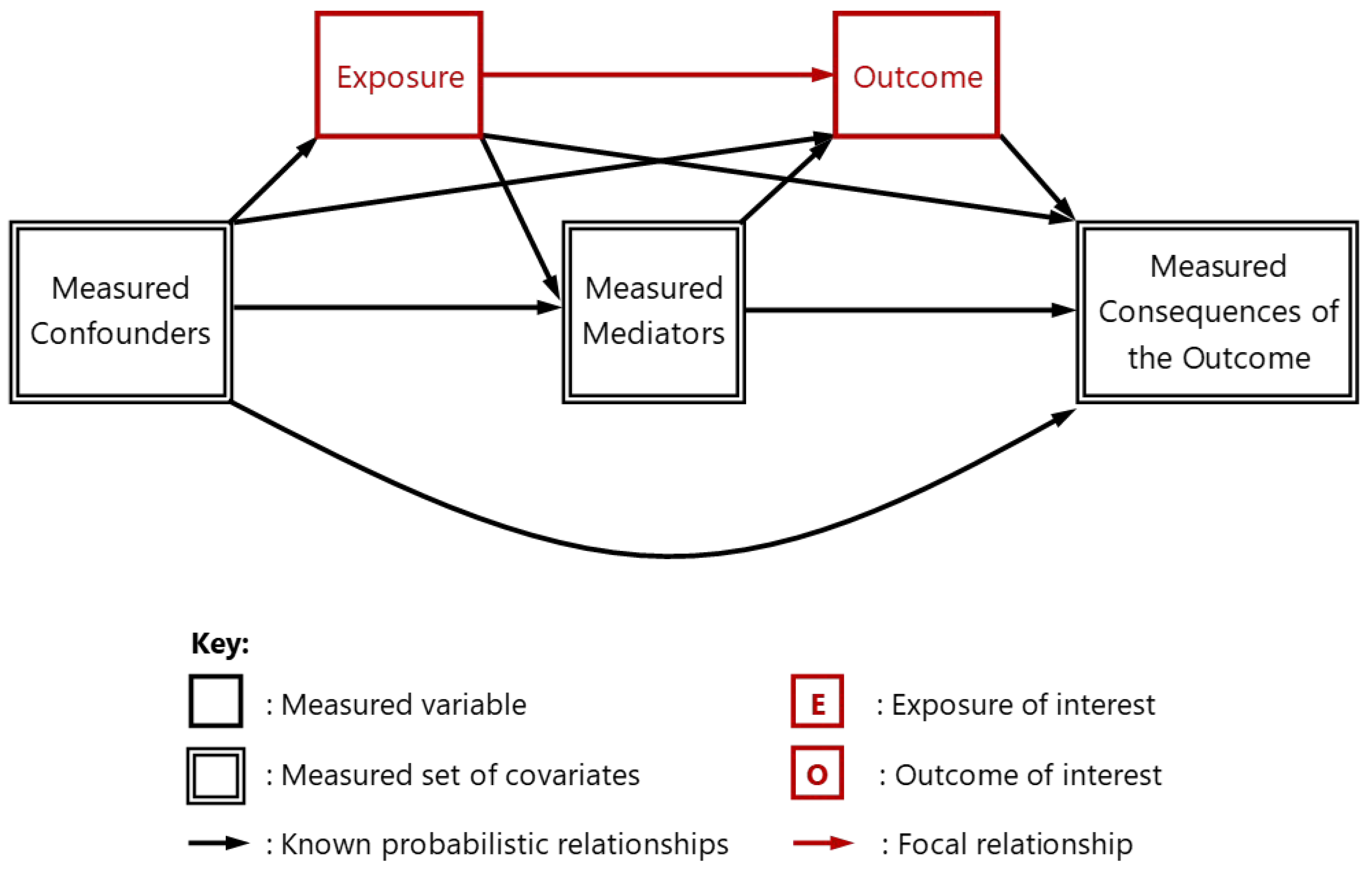
Figure 2.
A comprehensive or ‘universal’ DAG [6] summarizing all of the conceivable variables (both measured and unmeasured)1 that envelop the ‘focal relationship’ [21] between the specified ‘exposure’ (or ‘cause of interest’) and the specified ‘outcome’ (or ‘consequence of interest’ [22]). With the exception of the (specified) exposure and (specified) outcome variables, all other variables (commonly known as ‘covariates’) are represented here as ‘sets’ of variables (hence the double line surrounding these “super-nodes” [5]) to indicate that more than one such covariate is likely to co-occur during the period before the exposure (where these covariates operate as ‘confounders’), after the outcome (where the covariates concerned might best be described as ‘consequences of the outcome’), and the period in between (where the covariates involved are commonly known as ‘mediators’). Because some of the covariates within each set of measured covariates (indicated as rectangular shapes) and unmeasured covariates (indicated as spheroid shapes) might occur before or after one or more of those in another set of covariates, a comprehensive DAG of this nature includes some ostensibly ‘bi-directional’ causal paths that appear to operate in both directions, albeit between different variables within each set of (measured and unmeasured) ‘confounders’, ‘mediators’ and ‘consequences of the outcome’.
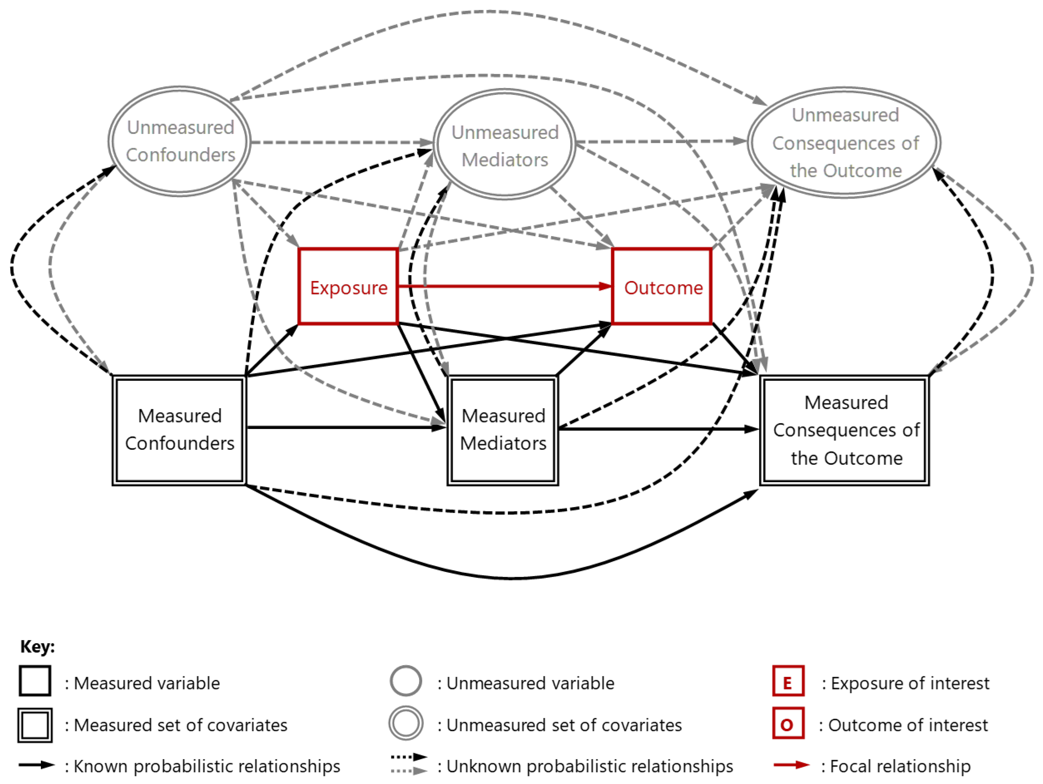
Figure 3.
A DAG redrawn from a published observational study exploring the possible causal relation between two alternative clinical procedures (thrombolysis vs. thrombectomy) and acute kidney injury [69] in which the potential, alternative temporal positions of six time-variant and time-invariant covariates (DM; CRF; CRT0; HCT0; SURG; and HCT1) have been highlighted using green boxes spanning the periods over which these covariates (as and when measured) might have plausibly occurred or crystallized. Note that, were SURG and/or the value of HCT1 to have occurred or crystallised after the value of CRT1 (as and when each of these values were measured), additional causal paths might then be required to reflect the plausible, probabilistic causal effects of CRT1/AKI and UK3 on SURG and/or HCT1 (as indicated by the two dashed arrows in green font [6]).
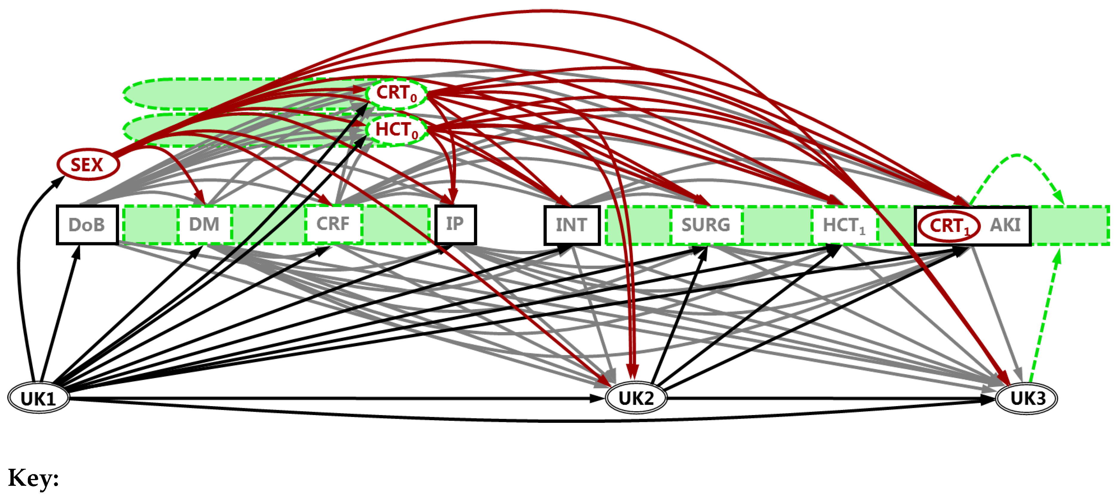
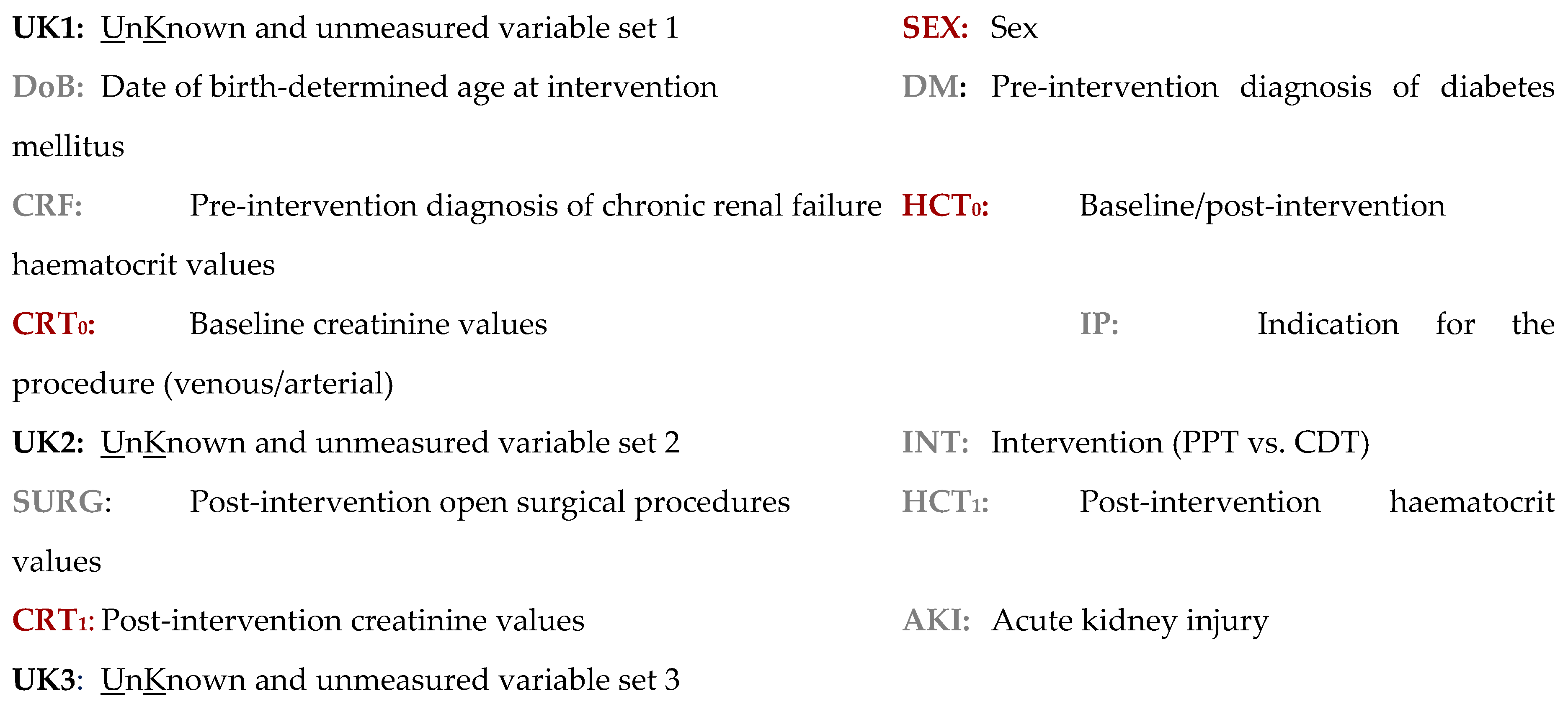
Figure 4.
Four simplifications of the 240+ alternative versions of the DAG presented in Figure 3 (and based on the same empirical study [6,69]) that are required to accommodate residual uncertainty in the temporal positioning of two key covariates (SURG; and HCT1) in which each of the measured (in grey font), unmeasured (in red font) and unacknowledged (in black font) covariates have been included in one of three discrete sets of variables, enclosed within separate boxes and located either: before the specified exposure variable (INT); after the specified outcome variable (AKI/CRT1); or in-between the two. This approach to simplifying DAGs reduces the very large number of alternative DAGs required to accommodate uncertainty in the temporal positioning of covariates therein, while retaining their utility for identifying those covariates that present a potential risk of analytical and inferential bias when estimating the sign, magnitude, precision or function of the specified focal relationship (in this instance between INT and CRT1/AKI). For key, see Figure 3 (above).
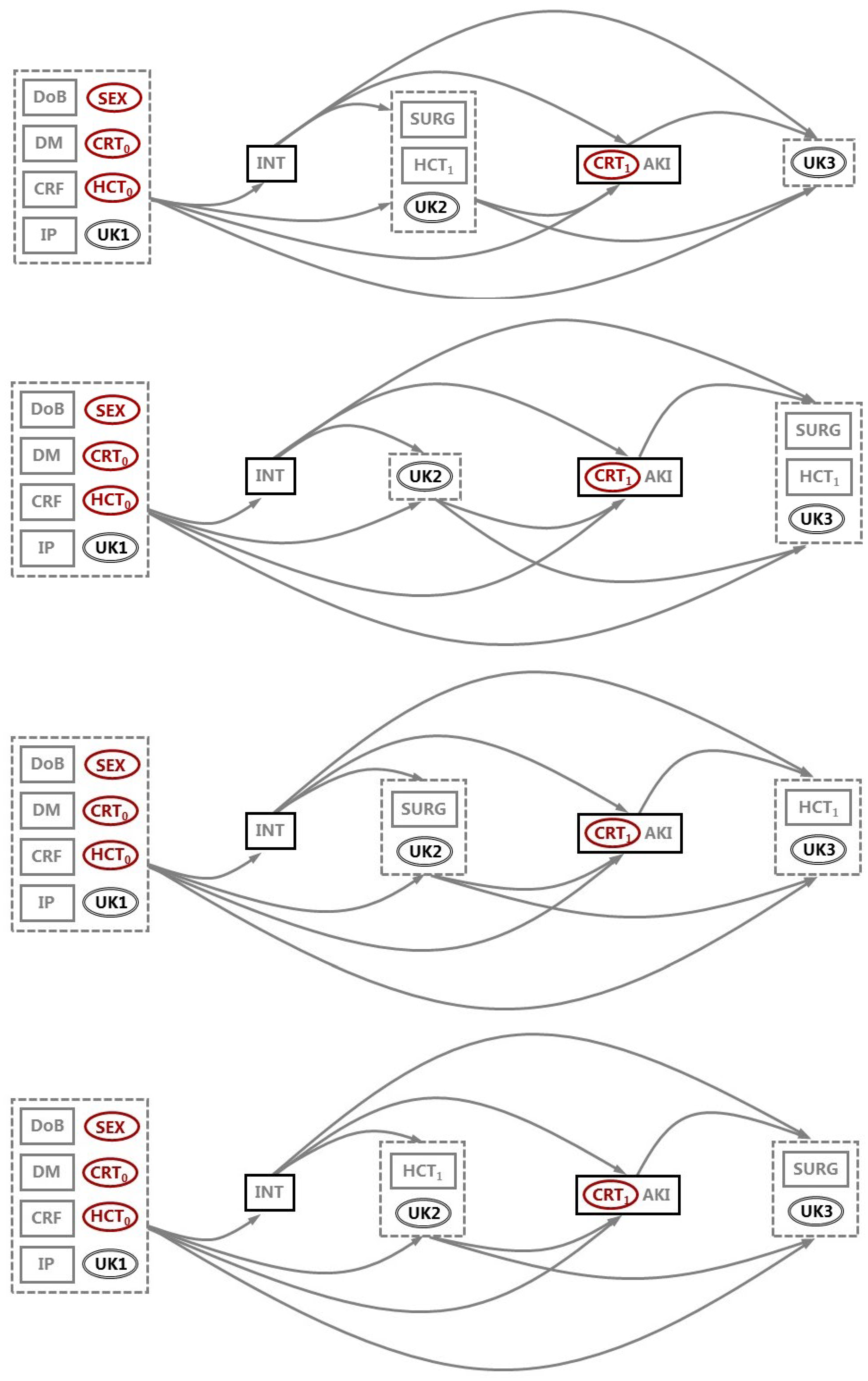
| 1 | Unmeasured variables are often termed ‘unknown’, ‘unobserved’ or ‘latent’ variables; while measured variables are occasionally termed ‘known’, ‘observed’ or ‘manifest’ variables |
| 2 | ‘Permissible paths’ are those paths that are consistent with directionality and acyclicity
|
| 3 | Although the aims of causal inference and prediction are very different – the former being concerned with mechanistic processes, the latter with classification/estimation – the temporal and contextual stability of many causal mechanisms makes understanding of these very useful for designing, developing and utilizing predictive algorithms in contexts/at times where the data-set generating processes might vary [24–27] |
Disclaimer/Publisher’s Note: The statements, opinions and data contained in all publications are solely those of the individual author(s) and contributor(s) and not of MDPI and/or the editor(s). MDPI and/or the editor(s) disclaim responsibility for any injury to people or property resulting from any ideas, methods, instructions or products referred to in the content. |
© 2025 by the authors. Licensee MDPI, Basel, Switzerland. This article is an open access article distributed under the terms and conditions of the Creative Commons Attribution (CC BY) license (http://creativecommons.org/licenses/by/4.0/).
Copyright: This open access article is published under a Creative Commons CC BY 4.0 license, which permit the free download, distribution, and reuse, provided that the author and preprint are cited in any reuse.


