Submitted:
08 June 2023
Posted:
09 June 2023
Read the latest preprint version here
Abstract
Sparse training (ST) aims to improve deep learning by replacing fully connected artificial neural networks (ANNs) with sparse ones, akin to the structure of brain networks. Therefore, it might benefit to borrow brain-inspired learning paradigms from complex network intelligence theory. Epitopological learning (EL) is a field of network science that studies how to implement learning on networks by changing the shape of their connectivity structure (epitopological plasticity). One way to implement EL is via link prediction: predicting the existence likelihood of nonobserved links in a network. Cannistraci-Hebb (CH) learning theory inspired the CH3-L3 network automata rule for link prediction which is effective for generalpurpose link prediction. Here, starting from CH3-L3 we propose Epitopological Sparse Ultra-deep Learning (ESUL) to apply EL into sparse training. In empirical experiments, we find that ESUL learns ANNs with sparse hyperbolic topology in which emerges a community layer organization that is ultra-deep (meaning that also each layer has an internal depth due to power-law node hierarchy). Furthermore, we discover that ESUL automatically sparse the neurons during training (arriving even to 30% neurons left in hidden layers), this process of node dynamic removal is called percolation. Then we design CH training (CHT), a training methodology that put ESUL at its heart, with the aim to enhance prediction performance. CHT consists of 4 parts: (i) correlated sparse topological initialization (CSTI), to initialize the network with a hierarchical topology; (ii) sparse weighting initialization (SWI), to tailor weights initialization to a sparse topology; (iii) ESUL, to shape the ANN topology during training; (iv) early stop with weight refinement, to tune only weights once the topology reaches stability. We conduct experiments on 6 datasets and 3 network structures (MLPs, VGG16, Transformer) comparing CHT to sparse training SOTA method and fully connected network. By significantly reducing the node size while retaining performance, CHT represents the first example of parsimony sparse training.
Keywords:
sparse training
; neural networks
; link prediction
; network automata
; Cannistraci-Hebb
; epitopological learning
1. Introduction
Over-parameterization [1] represents a significant advancement in deep learning. It has demonstrated that the loss function experiences a double descent phenomenon as the model complexity increases. This observation has facilitated the development of large models incorporating numerous modules and parameters to achieve superior performance. However, this approach places a significant burden on computational and storage resources, particularly for university researchers, small companies, and edge devices. As a result, researchers are currently focusing on methods to compress the model in order to increase its trade-off efficiency between performance and model size. There are many possible ways to compress a neural network, including Knowledge Distillation [2] to compress the model size, Model Quantification [3,4] to decrease the floating numbers during model training, sparse-based methods [5,6,7,8,9,10,11,12,13] to sparsify the connections in the model, and so on. Of all the compression-based methods, the sparse-based ones are the closest to the original design of Artificial Neural Networks (ANNs), which aim to imitate the structure of Brain Neural Networks (BNNs) where the connections in BNNs have already been proven to be extremely sparse. And in general, the sparse-based methods have shown good performance in various tasks [10] Current sparse-based methods can be divided into two categories: a) Pruning [5,6,7,8], which involves starting from a fully connected network and pruning the connections step by step; b) Sparse Training (ST), which begins with a sparsely connected network. Dynamic Sparse Training (DST)[9,10,11,12,13], a type of ST, is considered the most effective strategy as it can dynamically evolve the network topology. However, most DST algorithms only utilize the gradient information [10,13] or randomly assign new links [9,12] without considering and exploiting ANNs complex network topology. We believe that integrating topological network science (or, more specifically, brain-inspired learning paradigms from complex network intelligence theory) theories into DST could yield interesting results.
Epitopological Learning (EL)[14,15,16] is a field of network science inspired by the brain that explores how to implement learning on networks by changing the shape of their connectivity structure (epitopological plasticity). One approach to implement EL is via link prediction: predicting the existence likelihood of each non-observed link in a network. EL was developed alongside the Cannistraci-Hebb (CH) learning theory according to which: the sparse local-community organization of many complex networks (such as the brain ones) is coupled to a dynamic local Hebbian learning process and contains already in its mere structure enough information to predict how the connectivity will evolve during learning partially. Building upon CH3-L3 [17], one of the network automata rules under CH theory, we propose Epitopological Sparse Ultra-deep Learning (ESUL) to implement EL in evolving the topology of ANNs based on the DST procedure. Finally, we design CH training (CHT), a training methodology that put ESUL at its heart, with the aim of enhancing prediction performance. The experimental results show that CHT performs often better and trains faster than the SOTA dynamic sparse training algorithm. CHT reduces also the network node size significantly. Furthermore, in many experiments, CHT can equal or lightly outperform fully connected networks.
2. Related Work
In this section, we will introduce some basic notions of DST. Furthermore, we introduce epitopological learning and Cannistraci-Hebb theory for network automata link prediction, providing the knowledge to understand our proposed CHT methodology for ESUL in ANNs.
2.1. Dynamic Sparse Training
Dynamic Sparse Training (DST) is a novel training paradigm that can evolve the network structure efficiently for achieving better performance. It begins with a sparse initialized network and undergoes the removal and regrown procedure with multiple iterations. The main difference in modern DST methods is how to regrow the new links of the model. As summarized in Suppl. Table S1, there are two main streams of regrowth methods, random-based and gradient-based. random-based methods, such as SET [9], MEST [12], randomly assign new links to the network after removal, while gradient-based methods, such as RigL [10], extract the non-existing links with top-k absolute values of gradients. Generally, gradient-based methods perform better since they utilize more information from the learning process. However, the trade-off is that the backpropagation process of the gradient transformation is still fully connected. Recently, researchers are exploring ways to reduce the computation of the backpropagation process using gradient-based regrown [13] or designing some tricks to improve DST [11,12,18]. Therefore, in this paper, we introduce epitopological leaning, a new brain-inspired paradigm from network science, to evolve the sparse network topology.
Figure 1.
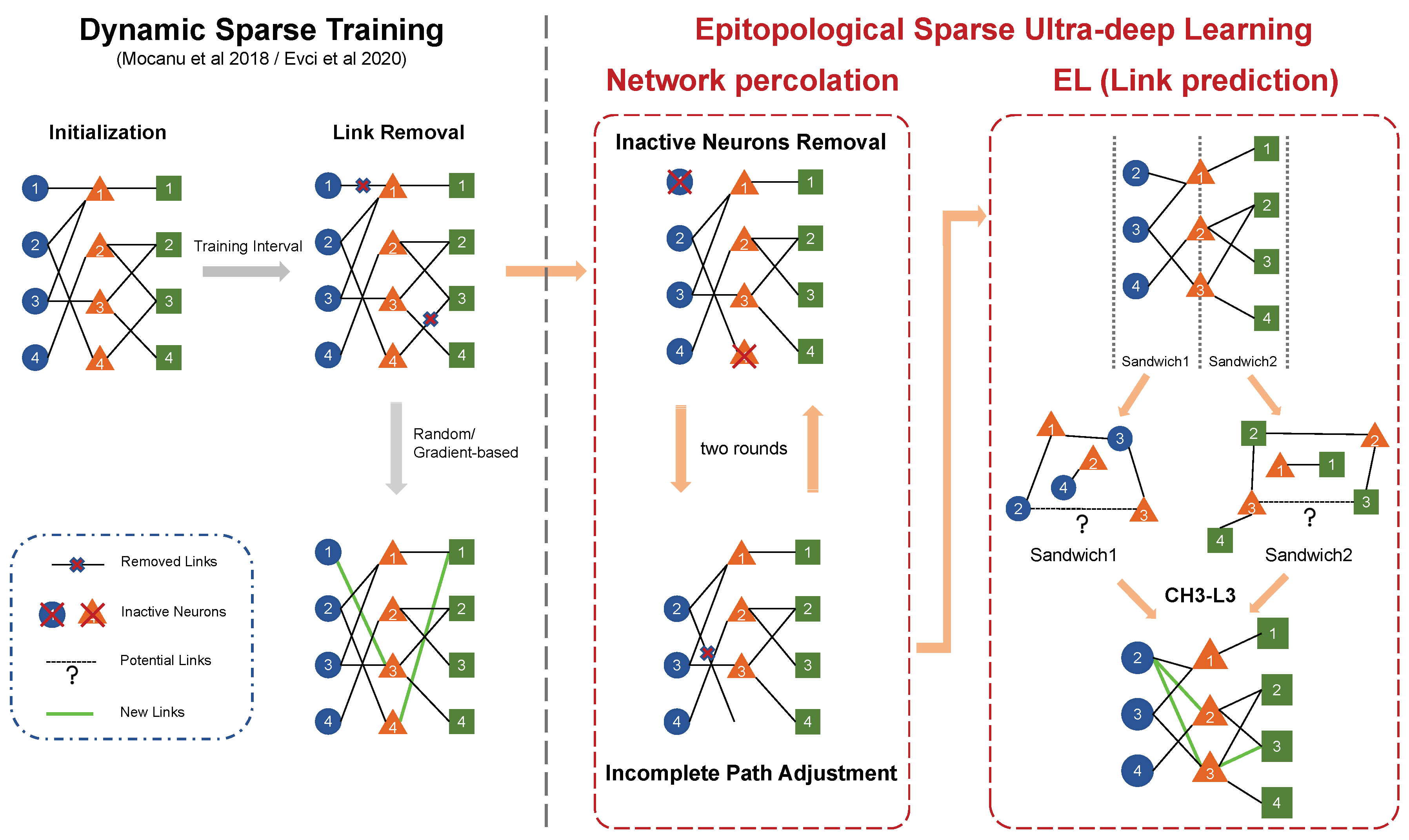
Illustration of the process of standard DST and ESUL. ESUL incorporates two additional steps for network evolution, namely network percolation and EL(link prediction). Network percolation involves inactive neurons removal (INR) and the adjustment of incomplete paths (IPA). In the epitopological learning (EL) part, which is based on link prediction, after dividing the entire network into several sandwich layers, the chosen link predictor separately calculates the link prediction score for each non-existing link and then regrows the top-k links in the same quantity as those removed.
Figure 1.
Illustration of the process of standard DST and ESUL. ESUL incorporates two additional steps for network evolution, namely network percolation and EL(link prediction). Network percolation involves inactive neurons removal (INR) and the adjustment of incomplete paths (IPA). In the epitopological learning (EL) part, which is based on link prediction, after dividing the entire network into several sandwich layers, the chosen link predictor separately calculates the link prediction score for each non-existing link and then regrows the top-k links in the same quantity as those removed.
2.2. Epitopological Learning and Cannistraci-Hebb Network Automata Theory for Link Prediction
Drawn from neurobiology, Hebbian learning was introduced in 1949 [19] and can be summarized in the axiom: “neurons that fire together wire together”. This could be interpreted in two ways: changing the synaptic weights (weight plasticity) and changing the shape of synaptic connectivity [14,15,16,20,21]. The latter is also called epitopological plasticity [20] because plasticity means “to change shape” and epitopological means “via a new topology”. Epitopological Learning (EL)[14,15,16] is derived from this second interpretation of Hebbian learning, and studies how to implement learning on networks by changing the shape of their connectivity structure. In this study, we adopt CH3-L3 [17] as link predictor to regrow the new links during the DST process. CH3-L3 is one of the best and most robust performing network automata which is inside Cannistraci-Hebb (CH) theory [17] that can automatically evolve the network topology with the given structure. The rationale of the CH theory is that, in any complex network with local-community organization, the cohort of nodes (neurons in the case of brain networks) tend to be co-activated (fire together) and to learn by forming new connections between them (wire together) because they are topologically isolated in the same local community [17]. CH3-L3 perfectly accomplishes this task by reducing the interaction with the nodes from the external community, which can be formalized as below:
where: u and v are the two seed nodes of the candidate interaction; , are the intermediate nodes on the considered path of length three; , are the respective external node degrees; and the summation is executed over all the paths of length three between the seed nodes u and v. The formula of is defined on path of any length, which adapts to any type of network organization [17]. Here, we consider because the topological regrowth process is implemented on each ANN sandwich layer separately, which has bipartite network topology organization. And, bipartite topology is based on the path of length 3 which displays a quadratic closure [14].
3. Epitopological Sparse Ultra-Deep Learning and Cannistraci-Hebb Training
3.1. Epitopological Sparse Ultra-Deep Learning
Following the second interpretation of the Hebbian Learning rule, we propose epitopological sparse ultra-deep Learning (ESUL), which implements EL in the sparse deep learning ANN. ESUL changes the perspective of training ANNs from weights to topology. ESUL focuses on the sparse topology of each sandwich layer, which is a bipartite sub-network composed of two consecutive layers of the ANN. The topological update formula for EL is:
Where represents the topology of the system at state n and represents the topology of the system at state . is the link predictor used by EL to predict the links between nodes in the network. In the standard DST process, as shown in Figure 1, there are three main steps: initialization, weight update, and network evolution, which include link removal and regrowth. ESUL follows initially the same steps of standard DST(Fig. 1, left side), but then progresses with substantial improvements (Fig. 1, right side): new removal part (network percolation), and new regrowth part (EL via link prediction). Firstly, in the removal phase, ESUL adopts the commonly used removal method that prunes links with lower absolute weights, which are considered less useful for the model’s performance. However, after the process of removing the lower magnitude weights, ESUL checks and corrects the topology for the presence of inactive neurons that either do not have a connection in one layer side or do not have any connections in both layer sides. When information passes through these inactive neurons, the forward and backward processes can get stuck. Moreover, if a node does not have any links in a bipartite network (i.e., a sandwich layer of the ANN), even if it has connections on the other side, no new links will be assigned to it in that network according to the formula of CH theory. Thus, ESUL implements the inactive neurons removal (INR) to ablate from the topology those inactive neurons. In particular, for the case that one node possesses connections on one layer side, we need to conduct incomplete path adjustment (IPA) that is to remove those links part of an incomplete path connected to the inactive neuron. Since IPA may produce some extra inactive neurons, we execute INR and IPA for two rounds. We termed the coupled process of INR and IPA as network percolation because it is reminiscent of the percolation theory in network science, which studies the connectivity behavior of networks when a fraction of the nodes or edges are removed [22]. If there are still some inactive neurons, we leave them in the network and clean up them during the next evolution. Once the network percolation is finished, EL via link prediction is implemented to regrow the links with higher link prediction scores. We repeat the process of removal and regrown after each learning weight update and until the network convergence to a stable topology. The steps of ESUL are explained in Suppl. Algorithm S1.
3.2. Cannistraci-Hebb Training
ESUL is a methodology that can work better when the network has already formed some relevant structural features. For instance, the fact that in each layer the nodes display a hierarchical position is associated with their degree. Nodes with higher degrees are network hubs in the layer and therefore they have a higher hierarchy. This hierarchy is facilitated by a hyperbolic network geometry with power-law-like node degree distribution [23]. In addition, the efficiency of the link predictor can be impaired by sparse random connectivity initialization. Therefore, we introduce below a strategy to initialize the sparse network topology and its weights. On the other hand, once the network topology has already stabilized (nodes removed and regrown are consistently similar), there may no longer be necessity to perform ESUL which could save the time of evolution. Therefore, to address these concerns, we propose a novel 4-step training procedure named Cannistraci-Hebb training (CHT).
Figure 2.
Main innovations introduced with CHT. A shows an example of how to construct the CSTI on the MNIST dataset, which involves four steps: vectorization, feature correlation, connectivity selection, and assembling topological hubbed network blocks. B presents a real network example of how SWI assigns weights to the sparse network. C displays the input layer degree distribution along with the associated heatmap on the MNIST figure template and the node degree distribution.
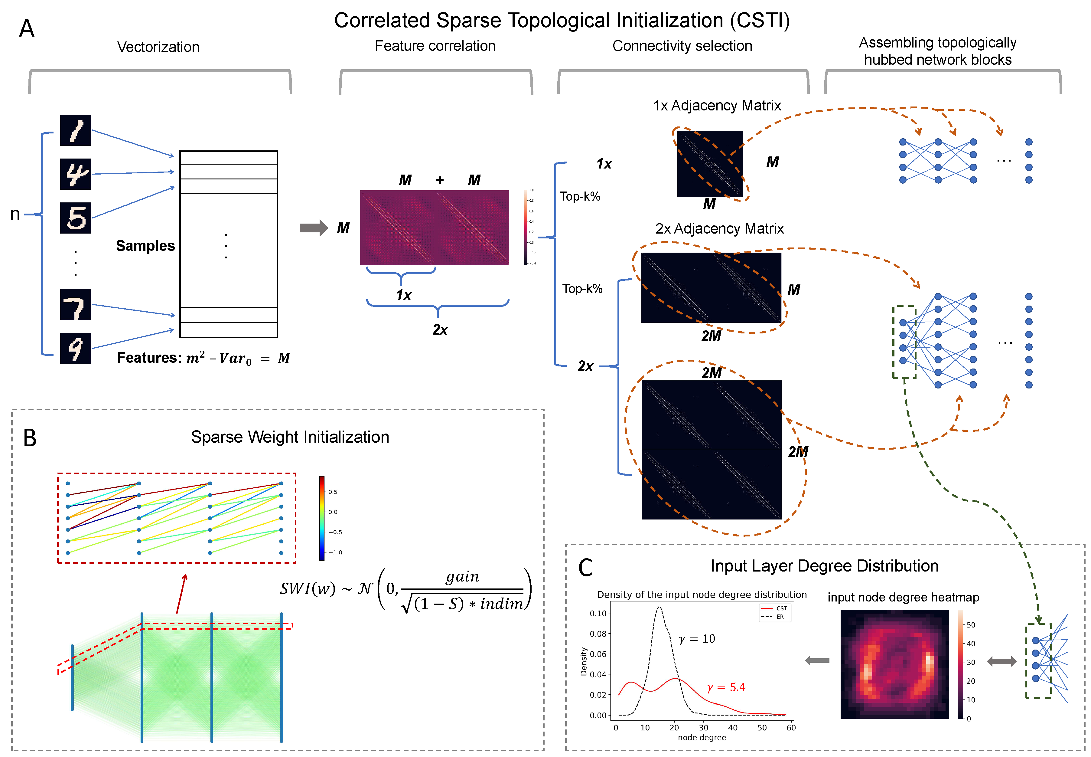
- Correlated sparse topological initialization (CSTI): as shown in Figure 2, CSTI consists of 4 steps. During the vectorization phase, we follow a specific procedure to construct a matrix of size n x M, where n represents the number of samples selected from the training set. Here, M denotes the number of valid features, obtained by excluding features with zero variance among the selected samples. Once we have this n x M matrix, we proceed with feature selection by calculating the Pearson Correlation for each feature. This step allows us to construct a correlation matrix. Subsequently, we construct a sparse adjacency matrix, where the positions marked with "1" (represented as white in the heatmap plot of Figure 2A) correspond to the top-k% values from the correlation matrix. The specific value of k depends on the desired sparsity level. This adjacency matrix plays a crucial role in defining the topology of each sandwich layer. The dimension of the hidden layer is determined by a scaling factor denoted as `x’. A scaling factor of 1x implies that the hidden layer’s dimension is equal to the input dimension, while a scaling factor of 2x indicates that the hidden layer’s dimension is twice the input dimension which allows the dimension of the hidden layer to be variable. In fact, since ESUL can efficiently reduce the dimension of each layer, the hidden dimension can automatically reduce to the inferred size. In this study we are only focusing on the sandwich layers in each model, in cases where sandwich layers cannot receive direct information from the input features, such as CNN and Transformer, we directly run the untrained network and use CSTI to initialize the adjacency matrix of each layer. The detailed implementation of VGG16 and Transformer can be found in the supplementary material.
-
Sparse Weight Initialization (SWI): in addition to the topological initialization, we also recognize the importance of weight initialization in the sparse network. The standard initialization methods such as Kaiming [24] or Xavier [25] are designed to keep the variance of the values consistent across layers. However, these methods are not suitable for sparse network initialization since the variance is not consistent with the previous layer. To address this issue, we propose a method that can assign initial weights in any sparsity cases. SWI can also be extended to the fully connected network, in which case it becomes equivalent to Kaiming initialization. Here we provide the mathematical formula for SWI and in supplementary we provide the rationale that brought us to its definition.denotes the normal distribution with a mean of 0 and a variance of . The value of varies for different activation functions. In this article, except for Transformer, all other models use ReLU, where the gain is always . S here denotes the desired sparsity and indicates the input dimension of each sandwich layer.
- Epitopological prediction: this step corresponds to ESUL (introduced in Section 3.1), but evolves the sparse topological structure starting from CSTI + SWI initialization rather than random.
- Early stop and weight refinement: during the process of epitological prediction, it is common to observe an overlap between the links that are removed and added, as shown in the last plot in Suppl. Figure S2D. After several rounds of topological evolution, the overlap rate can reach a high level, indicating that the network has achieved a relatively stable topological structure. In this case, the ESUL algorithm may continuously remove and add mostly the same links, which can slow down the training process. To solve this problem, we introduce an early stop mechanism for each sandwich layer. When the overlap rate between the removed and added links reaches a certain threshold (we use a significant level of 90%), we stop the epitopological prediction for that layer. Once all the sandwich layers have reached the early stopping condition, the model starts to focus on learning and refining the weights using the obtained network structure.
4. Results
In this section, we present the experimental results obtained by applying ESUL and CHT on 6 datasets (MNIST [26], Fashion_MNIST [27], EMNIST [28], CIFAR10 [29], CIFAR100 [29], and Multi-30K [30]) using 3 different network architectures (MLP, VGG16 [31], and Transformer [32]) to evaluate their performance compared to DST methods and fully connected networks. All the experiments are using 3 random seeds and the hyperparameter settings are reported in the Suppl. Table S2. All experiments are with 99% sparsity since we want to investigate extremely sparse learning scenarios and compare them with fully connected ones.
4.1. Results of ESUL
In this section, we aim to investigate the effectiveness of ESUL from a network science perspective. We utilize the framework of ESUL and compare CH3-L3 (the proposed topological link prediction-based regrown method) with randomly assigning new links (which is typical of SET [9]). We run all the experiments with the default hyperparameter setting as shown in Suppl. Table 2, and conduct experiments on 5 datasets: MNIST, Fashion_MNIST, EMNIST using MLP and CIFAR10, CIFAR100 using VGG16. For the first 3 datasets, we adopt MLP with an architecture of 784-1000-1000-1000-10 (47 output neurons for EMNIST), while for VGG16, we replace the fully connected layers after the convolution layers with the sparse network and assign them a structure of 512-1000-1000-1000-10 (100 output neurons for CIFAR100). Figure 3 compares the performance of CH3-L3 (ESUL) and random (SET) on the five datasets. The first row shows the accuracy curves of each algorithm and on the upper right corner of each panel, we mark the accuracy improvement at the 250th epoch. The second row of Figure 3 shows the Area Across the Epochs (AAE), which reflects the learning speed of each algorithm. The computation and explanation of AAE can be found in the supplementary material. Based on the results of the accuracy curve and AAE values, CH3-L3 (ESUL) outperforms random (SET) on all the datasets, demonstrating that the proposed epitopological learning method is effective in identifying lottery tickets, and CH theory is boosting deep learning.
Figure 4A provides evidence that the sparse network trained with ESUL can automatically percolate the network to a significantly smaller size and form a hyperbolic network with community organizations. The example network structure of MNIST dataset on MLP is presented, where each block shows a plain representation and a hyperbolic representation of each network at the initial (that is common) and the final epoch status (that is random (SET) or CH3-L3 (ESUL)). The ESUL block in Figure 4A shows that each layer of the network has been percolated to a small size, especially the middle two hidden layers where the active neuron post-percolation rate (ANP) has been reduced to less than 20%. This indicates that the network trained by ESUL can achieve better performance with significantly fewer active neurons and that the size of the hidden layers can be automatically learned by the topological evolution of ESUL. ANP is particularly significant in deep learning because neural networks often have a large number of redundant neurons that do not contribute significantly to the model’s performance. ESUL can reduce the computational cost of training and inference, making the network more efficient and scalable. In addition, reducing the number of active neurons can also help to prevent overfitting and improve the generalization ability of the model which remarkably reduces the dimensionality of the embedding in the hidden layers.
Figure 3.
The comparison of CH3-L3 (ESUL) and random (SET). In the first row, we report the accuracy curves of CH3-L3 and random on 5 datasets and mark the increment at the 250th epoch on the upper right corner of each panel. The second row reports the value of area across the epochs (AAE) which indicates the learning speed of different algorithms corresponding to the upper ACC plot.
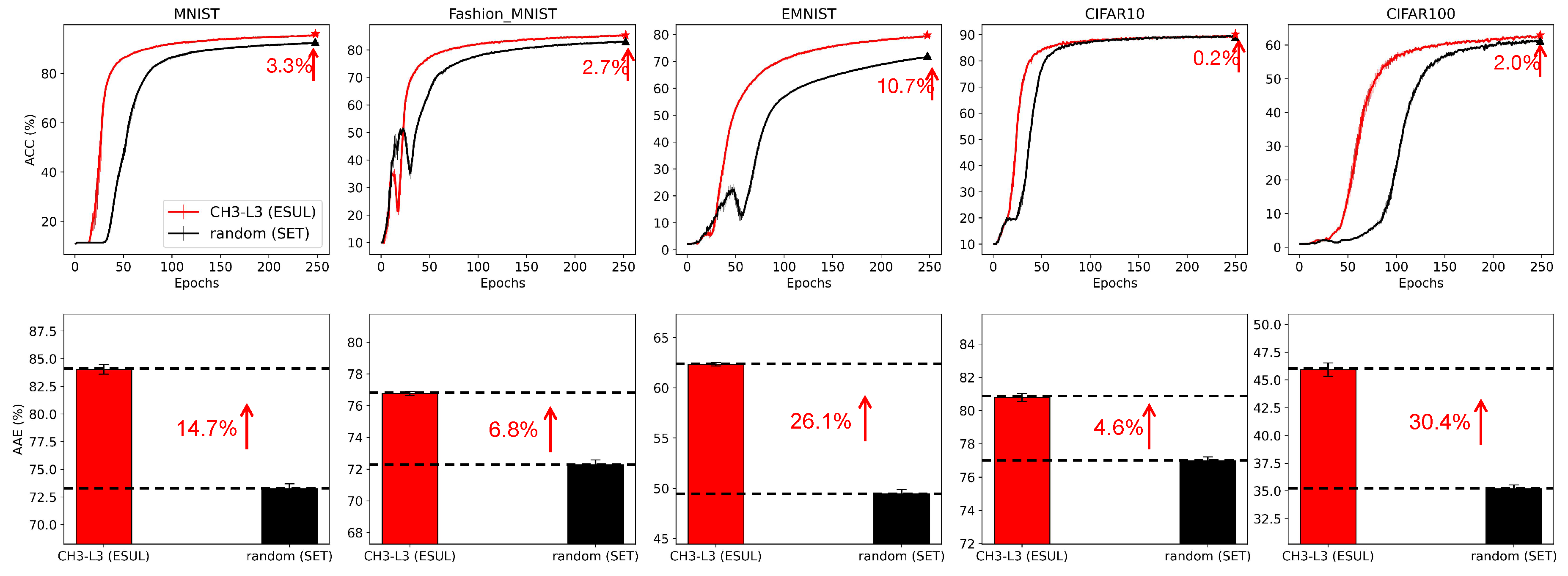
Figure 4.
Network science analysis of the sparse ANNs topology. A shows the presentation of different statuses of the network, including the network initialized by ER, the network trained by random (final epoch), and the network trained by ESUL (final epoch). The angular separability index (ASI) and power law exponent are reported in each panel. Additionally, the active neuron post-percolation rate (ANP) curve across the epochs is reported inside the ESUL panel. B shows the 4 network topological measures averaged on 5 different ANNs, trained in 5 datasets by CH3-L3 (ESUL) and random (SET), the shadow area means the standard error of the 5 datasets.
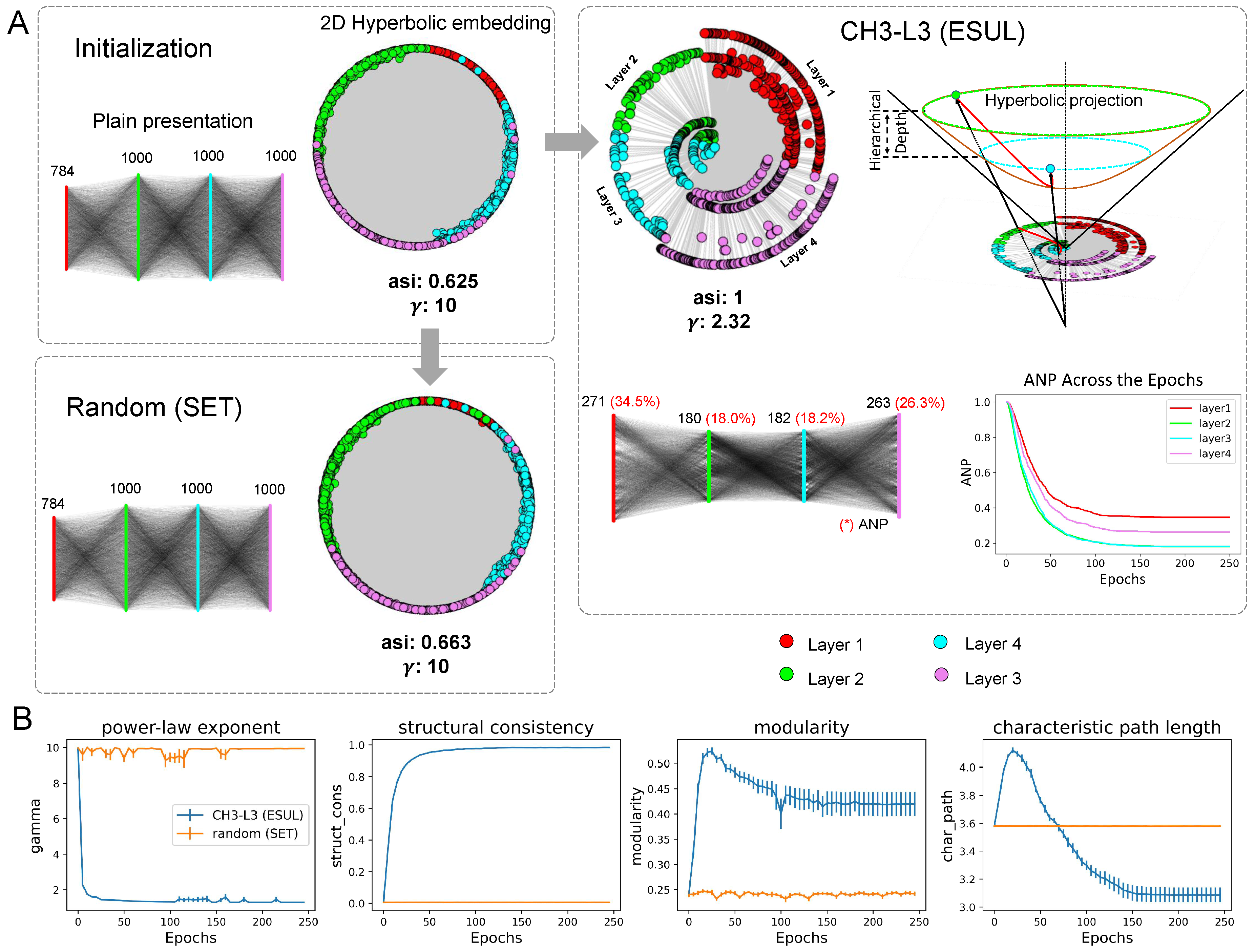
Furthermore, we perform coalescent embedding [33] of each network in Figure 4A into the hyperbolic space, where the radial coordinates are associated with node degree hierarchical power-law-like distribution and the angular coordinates with geometrical proximity of the nodes in the latent space. This means that the typical tree-like structure of the hyperbolic network emerges if the node degree distribution is power law ([23]). Indeed, the more power-law in the network, the more the nodes migrated towards the center of the hyperbolic 2D representation, and the more the network displays a hierarchical hyperbolic structure.
Surprisingly, we found that the network formed by CH3-L3 finally (at the 250th epoch) becomes a hyperbolic power law () network with a hyperbolic community organization (angular separability index, ASI = 1, indicating a perfect angular separability of the community formed by each layer [34]), while the others (initial and random at the 250th epoch) do not display either power law () topology with latent hyperbolic geometry or crystal-clear community organization (ASI around 0.6 denotes a substantial presence of aberration in the community organization [34]). Community organization is a fundamental mesoscale structure of real complex networks [35] such as biological and socioeconomical [36]. For instance, brain networks [37] and maritime networks [38] display distinctive community structure that is fundamental to facilitating diversified functional processing in each community separately and global sharing to integrate these functionalities between communities. ESUL approach can not only efficiently identify the important neurons but also learn a more complex and ultra-deep network structure. This mesoscale structure leverages topologically separated layer-community to implement in each of them diversified and specialized functional processing. The result of this ‘regional’ layer-community processing is then globally integrated together via the hubs (nodes with higher degrees) that each layer-community owns. Thanks to the power-law distributions, regional hubs that are part of each regional layer-community emerge as ultra-deep nodes in the global network structure and promote a hierarchical organization that makes the networks ultra-small-world (as we will explain a few lines below). Indeed, in Figure 4A left we show that the community layer organization of the ESUL learned network is ultra-deep, meaning that also each layer has an internal hierarchical depth due to power-law node degree hierarchy. Nodes with higher degrees in each layer community are also more central and cross-connected in the entire network topology playing a central role (their radial coordinate is smaller) in the latent hyperbolic space which underlies the network topology. It is as the ANN has an ultra-depth that is orthogonal to the regular plan layer depth. The regular plan depth is given by the organization in layers, the ultra-depth is given by the topological centrality of different nodes from different layers in the hyperbolic geometry that underlies the ANN trained by ESUL. Moreover, we present the analysis of the ANP reduction throughout the epochs within the ESUL blocks. From our results, it is evident that the ANP diminishes to a significantly low level after approximately 50 evolution iterations. This finding highlights the efficient network percolation capability of ESUL, while in the meantime it suggests that a prolonged network evolution may not be necessary for ESUL, as the network stabilizes within a few epochs, indicating its rapid convergence.
To evaluate the structural properties of the sparse network, we utilize measures commonly used in network science (Figure 4B). The details of each measure are explained in the supplementary material, and here we will focus on the observed phenomena. We consider the entire ANN network topology and compare the average values in 5 datasets of CH3-L3 (ESUL) with random (SET) using 4 network topological measures. The plot of power-law gamma indicates that CH3-L3 (ESUL) produces networks with power-low degree distribution (), whereas random (SET) does not. We want to clarify that Mocanu et al. [9] also reported that SET could achieve a power-law distribution with MLPs but in their case, they used the learning rate of 0.01 and extended the learning epochs to 1000. We acknowledge that maybe with a higher learning rate and a much longer waiting time, SET can achieve a power-law distribution. However, we emphasize that in Figure 4B (first panel) ESUL achieves power-law degree distribution regardless of the conditions in 5 different datasets and 2 types (MLPs, VGG16) of network architecture. This is because ESUL regrows connectivity based on the existing network topology according to a brain-network automaton rule, instead SET regrows at random. Furthermore, structure consistency [39] implies that CH3-L3 (ESUL) makes the network more predictable, while modularity shows that it can form distinct obvious communities. The characteristic path length is computed as the average node-pairs length in the network, it is a measure associated with network small-worldness and express also message passing and navigability efficiency of a network [23]. ESUL-trained network topology is ultra-small-world, which happens when a network is small-world with power-law degree exponent lower than 3 (more precisely closer to 2 than 3)[23], and this means that the transfer of information or energy in the network is even more efficient than a regular small-world network [23]. All of these measures give strong evidence that ESUL is capable of transforming the original random network into a complex structured topology that is more suitable for training and potentially a valid lottery-ticket network [8]. This transformation can lead to significant improvements in network efficiency, scalability, and performance.
4.2. Results of CHT

Table 1.
Result of CHT comparing to RigL and Fully connected network on 1x and 2x cases
| MNIST(MLP) | Fashion_MNIST(MLP) | EMNIST(MLP) | ||||
|---|---|---|---|---|---|---|
| ACC | AAE | ACC | AAE | ACC | AAE | |
| FC | 98.69±0.02 | 96.33±0.16 | 90.43±0.09 | 87.40±0.02 | 85.58±0.06 | 81.75±0.10 |
| RigL | 97.40±0.07 | 93.69±0.10 | 88.02±0.11 | 84.49±0.12 | 82.96±0.04 | 78.01±0.06 |
| CHT | 98.05±0.04 | 95.45±0.05 | 88.07±0.11 | 85.20±0.06 | 83.82±0.04 | 80.25±0.20 |
| FC | 98.73±0.03 | 96.27±0.13 | 90.74±0.13 | 87.58±0.04 | 85.85±0.05 | 82.19±0.12 |
| RigL | 97.91±0.09 | 94.25±0.03 | 88.66±0.07 | 85.23±0.08 | 83.44±0.09 | 79.10±0.25 |
| CHT | 98.34±0.08 | 95.60±0.05 | 88.34±0.07 | 85.53±0.25 | 85.43±0.10 | 81.18±0.15 |
| CIFAR10(VGG16) | CIFAR100(VGG16) | Multi30K(Transformer) | ||||
| ACC | AAE | ACC | AAE | BLEU | AAE | |
| FC | 91.52±0.04 | 87.74±0.03 | 66.73±0.06 | 57.21±0.11 | 24.0±0.20 | 20.9±0.13 |
| RigL | 91.60±0.10* | 86.54±0.14 | 67.87±0.17* | 53.80±0.49 | 21.1±0.08 | 18.1±0.08 |
| CHT | 91.68±0.15* | 86.57±0.08 | 67.58±0.30* | 57.30±0.20* | 21.3±0.29 | 18.3±0.13 |
| FC | 91.75±0.07 | 87.86±0.02 | 66.34±0.06 | 57.02±0.04 | - | - |
| RigL | 91.75±0.03 | 87.07±0.09 | 67.88±0.35* | 54.08±0.43 | - | - |
| CHT | 91.98±0.03* | 88.29±0.10* | 67.70±0.16* | 57.79±0.08* | - | - |
To enhance the performance of ESUL, we propose a 4-step procedure named CHT. We first report the initialization structure in Figure 2C which is a CSTI example with 2x version of MNIST dataset, we construct the heatmap of the input layer degrees and node distribution density curve. It can be clearly observed that with CSTI, the links are assigned to nodes mostly associated with input pixels in the center of figures in the MNIST dataset, and indeed the area at the center of the figures is more informative. We also report the CSTI-formed network has an initialized power law exponent which indicates a topology with more hub nodes than in a random network with . To assess the effectiveness of each process (excluding ESUL which was investigated in the previous section) proposed by CHT, we conducted an ablation test and reported the results in the first three plots of Suppl. Figure S2. These experiments demonstrate the utility of each individual component within the CHT framework.
In Table 1, we report the final performance of CHT compared to the SOTA DST method RigL and fully connected network on 6 datasets and 3 different models. Based on the obtained results, it is evident that CHT outperforms RigL in the majority of cases and consistently achieves faster training. The analysis of running time and FLOPs please refer to the Suppl. Table S3. Furthermore, we achieve comparable results to the Fully Connected (FC) model, with only 1% of the links remaining, on both the MNIST and EMNIST datasets. Moreover, note that while our performance is comparable to RigL on the CIFAR100 dataset, we observe higher AAE in our approach, indicating that CHT exhibits faster learning capabilities.
Table 2.
Active neuron post-percolation rate corresponding to the results in Table 1
| MNIST | Fashion_MNIST | EMNIST | CIFAR10 | CIFAR100 | Multi-30k | |
|---|---|---|---|---|---|---|
| CHT | 31.15% | 30.45% | 42.22% | 32.52% | 32.32% | 33.86% |
| RigL | 97.45% | 98.69% | 89.19% | 94.14% | 93.50% | 88.7% |
| CHT | 33.27% | 29.25% | 39.78% | 34.24% | 35.71% | - |
| RigL | 100% | 100% | 99.82% | 99.83% | 99.80% | - |
Additionally, as illustrated in Table 2, CHT successfully percolated the network to a range of 30-40% of the original neurons in every dataset. This implies that, from a logical standpoint, we utilize fewer neurons to achieve similar results as RigL, therefore CHT can generalize and abstract better in the hidden layers of the data information associated with the classification task, providing a new solution to find the Lottery Ticket of ANNs [8]. CHT’s result to adaptively percolate the network size providing a minimalistic network modeling that preserves performance with a smaller architecture is a typical solution in line with Occam’s razor also named in science as the principle of parsimony, which is the problem-solving principle advocating to search for explanations constructed with the smallest possible set of elements [40]. For instance, in physics, parsimony was an important heuristic in Albert Einstein’s formulation of special relativity [41]; Pierre Louis Maupertuis’ and Leonhard Euler’s work on the principle of least action [42]; and Max Planck, Werner Heisenberg and Louis de Broglie development of quantum mechanics [43,44]. On this basis, we can claim that CHT represents the first example of an algorithm for “parsimony sparse training”.
References
- Belkin, M.; Hsu, D.; Ma, S.; Mandal, S. Reconciling modern machine-learning practice and the classical bias–variance trade-off. Proc. Natl. Acad. Sci. 2019, 116, 15849–15854. [Google Scholar] [CrossRef]
- Hinton, G.E.; Vinyals, O.; Dean, J. Distilling the Knowledge in a Neural Network. CoRR, 1503. [Google Scholar] [CrossRef]
- Han, S.; Mao, H.; Dally, W.J. Deep Compression: Compressing Deep Neural Network with Pruning, Trained Quantization and Huffman Coding. 4th International Conference on Learning Representations, ICLR 2016, San Juan, Puerto Rico, -4, 2016, Conference Track Proceedings; Bengio, Y.; LeCun, Y., Eds., 2016. 2 May. [CrossRef]
- Chen, W.; Wilson, J.T.; Tyree, S.; Weinberger, K.Q.; Chen, Y. Compressing Neural Networks with the Hashing Trick. Proceedings of the 32nd International Conference on Machine Learning, ICML 2015, Lille, France, 6-; Bach, F.R.; Blei, D.M., Eds. JMLR.org, 2015, Vol. 37, JMLR Workshop and Conference Proceedings, pp. 2285–2294. 11 July.
- LeCun, Y.; Denker, J.S.; Solla, S.A. Optimal Brain Damage. Advances in Neural Information Processing Systems 2, [NIPS Conference, Denver, Colorado, USA, -30, 1989]; Touretzky, D.S., Ed. Morgan Kaufmann, 1989, pp. 598–605. 27 November.
- Han, S.; Pool, J.; Tran, J.; Dally, W.J. Learning both Weights and Connections for Efficient Neural Network. Advances in Neural Information Processing Systems 28: Annual Conference on Neural Information Processing Systems 2015, -12, 2015, Montreal, Quebec, Canada; Cortes, C.; Lawrence, N.D.; Lee, D.D.; Sugiyama, M.; Garnett, R., Eds., 2015, pp. 1135–1143. 7 December.
- Lee, N.; Ajanthan, T.; Torr, P.H.S. Snip: Single-Shot Network Pruning based on Connection sensitivity. 7th International Conference on Learning Representations, ICLR 2019, New Orleans, LA, USA, -9, 2019. OpenReview.net, 2019. 6 May.
- Frankle, J.; Carbin, M. The Lottery Ticket Hypothesis: Finding Sparse, Trainable Neural Networks. 7th International Conference on Learning Representations, ICLR 2019, New Orleans, LA, USA, -9, 2019. OpenReview.net, 2019. 6 May.
- Mocanu, D.C.; Mocanu, E.; Stone, P.; Nguyen, P.H.; Gibescu, M.; Liotta, A. Scalable training of artificial neural networks with adaptive sparse connectivity inspired by network science. Nat. Commun. 2018, 9, 1–12. [Google Scholar] [CrossRef]
- Evci, U.; Gale, T.; Menick, J.; Castro, P.S.; Elsen, E. Rigging the Lottery: Making All Tickets Winners. Proceedings of the 37th International Conference on Machine Learning, ICML 2020, 13-, Virtual Event. PMLR, 2020, Vol. 119, Proceedings of Machine Learning Research, pp. 2943–2952. 18 July.
- Liu, S.; Yin, L.; Mocanu, D.C.; Pechenizkiy, M. Do We Actually Need Dense Over-Parameterization? In-Time Over-Parameterization in Sparse Training. Proceedings of the 38th International Conference on Machine Learning, ICML 2021, 18-, Virtual Event; Meila, M.; Zhang, T., Eds. PMLR, 2021, Vol. 139, Proceedings of Machine Learning Research, pp. 6989–7000. 24 July.
- Yuan, G.; Ma, X.; Niu, W.; Li, Z.; Kong, Z.; Liu, N.; Gong, Y.; Zhan, Z.; He, C.; Jin, Q.; others. Mest: Accurate and fast memory-economic sparse training framework on the edge. Adv. Neural Inf. Process. Syst. 2021, 34, 20838–20850. [Google Scholar]
- Liu, S.; Chen, T.; Chen, X.; Atashgahi, Z.; Yin, L.; Kou, H.; Shen, L.; Pechenizkiy, M.; Wang, Z.; Mocanu, D.C. Sparse Training via Boosting Pruning Plasticity with Neuroregeneration. 2021, pp. 9908–9922.
- Daminelli, S.; Thomas, J.M.; Durán, C.; Cannistraci, C.V. Common neighbours and the local-community-paradigm for topological link prediction in bipartite networks. New J. Phys. 2015, 17, 113037. [Google Scholar] [CrossRef]
- Durán, C.; Daminelli, S.; Thomas, J.M.; Haupt, V.J.; Schroeder, M.; Cannistraci, C.V. Pioneering topological methods for network-based drug–target prediction by exploiting a brain-network self-organization theory. Briefings Bioinform. 2017, 19, 1183–1202. [Google Scholar] [CrossRef] [PubMed]
- Cannistraci, C.V. Modelling Self-Organization in Complex Networks Via a Brain-Inspired Network Automata Theory Improves Link Reliability in Protein Interactomes. Sci Rep 2018, 8, 2045–2322. [Google Scholar] [CrossRef]
- Muscoloni, A.; Michieli, U.; Cannistraci, C. Adaptive Network Automata Modelling of Complex Networks. preprints 2020. [Google Scholar]
- Yuan, G.; Li, Y.; Li, S.; Kong, Z.; Tulyakov, S.; Tang, X.; Wang, Y.; Ren, J. Layer Freezing & Data Sieving: Missing Pieces of a Generic Framework for Sparse Training. arXiv preprint arXiv:2209.11204, arXiv:2209.11204 2022.
- Hebb, D. The Organization of Behavior. emphNew York, 1949.
- Cannistraci, C.V.; Alanis-Lobato, G.; Ravasi, T. From link-prediction in brain connectomes and protein interactomes to the local-community-paradigm in complex networks. Sci. Rep. 2013, 3, 1613. [Google Scholar] [CrossRef] [PubMed]
- Narula, V.e.a. Can local-community-paradigm and epitopological learning enhance our understanding of how local brain connectivity is able to process, learn and memorize chronic pain? Appl. Netw. Sci. 2017, 2. [Google Scholar] [CrossRef]
- Li, M.; Liu, R.R.; Lü, L.; Hu, M.B.; Xu, S.; Zhang, Y.C. Percolation on complex networks: Theory and application. Phys. Rep. 2021, 907, 1–68. [Google Scholar] [CrossRef]
- Cannistraci, C.V.; Muscoloni, A. Geometrical congruence, greedy navigability and myopic transfer in complex networks and brain connectomes. Nat. Commun. 2022, 13, 7308. [Google Scholar] [CrossRef] [PubMed]
- He, K.; Zhang, X.; Ren, S.; Sun, J. Delving deep into rectifiers: Surpassing human-level performance on imagenet classification. Proceedings of the IEEE international conference on computer vision, 2015, pp. 1026–1034.
- Glorot, X.; Bengio, Y. Understanding the difficulty of training deep feedforward neural networks. Proceedings of the Thirteenth International Conference on Artificial Intelligence and Statistics, AISTATS 2010, Chia Laguna Resort, Sardinia, Italy, -15, 2010; Teh, Y.W.; Titterington, D.M., Eds. JMLR.org, 2010, Vol. 9, JMLR Proceedings, pp. 249–256. 13 May.
- LeCun, Y.; Bottou, L.; Bengio, Y.; Haffner, P. Gradient-based learning applied to document recognition. Proc. IEEE 1998, 86, 2278–2324. [Google Scholar] [CrossRef]
- Xiao, H.; Rasul, K.; Vollgraf, R. Fashion-mnist: A novel image dataset for benchmarking machine learning algorithms. arXiv preprint arXiv:1708.07747, arXiv:1708.07747 2017. [CrossRef]
- Cohen, G.; Afshar, S.; Tapson, J.; Van Schaik, A. EMNIST: Extending MNIST to handwritten letters. 2017 international joint conference on neural networks (IJCNN). IEEE, 2017, pp. 2921–2926. [CrossRef]
- Krizhevsky, A. Learning Multiple Layers of Features from Tiny Images 2009. pp. 32–33.
- Elliott, D.; Frank, S.; Sima’an, K.; Specia, L. Multi30K: Multilingual English-German Image Descriptions. Proceedings of the 5th Workshop on Vision and Language. Association for Computational Linguistics, 2016, pp. 74. [CrossRef]
- Simonyan, K.; Zisserman, A. Very deep convolutional networks for large-scale image recognition. arXiv preprint arXiv:1409.1556, arXiv:1409.1556 2014. [CrossRef]
- Vaswani, A.; Shazeer, N.; Parmar, N.; Uszkoreit, J.; Jones, L.; Gomez, A.N.; Kaiser. ; Polosukhin, I. Attention is all you need. Adv. Neural Inf. Process. Syst. 2017, 30. [Google Scholar]
- Muscoloni, A.; Thomas, J.M.; Ciucci, S.; Bianconi, G.; Cannistraci, C.V. Machine learning meets complex networks via coalescent embedding in the hyperbolic space. Nat. Commun. 2017, 8, 1615. [Google Scholar] [CrossRef] [PubMed]
- Muscoloni, A.; Cannistraci, C.V. Angular separability of data clusters or network communities in geometrical space and its relevance to hyperbolic embedding. arXiv preprint arXiv:1907.00025, arXiv:1907.00025 2019. [CrossRef]
- Muscoloni, A.; Cannistraci, C.V. A nonuniform popularity-similarity optimization (nPSO) model to efficiently generate realistic complex networks with communities. New J. Phys. 2018, 20, 052002. [Google Scholar] [CrossRef]
- Durán, C.; Muscoloni, A.; Cannistraci, C.V. Geometrical inspired pre-weighting enhances Markov clustering community detection in complex networks. Appl. Netw. Sci. 2021, 6, 1–16. [Google Scholar] [CrossRef]
- Cacciola, A.; Muscoloni, A.; Narula, V.; Calamuneri, A.; Nigro, S.; Mayer, E.A.; Labus, J.S.; Anastasi, G.; Quattrone, A.; Quartarone, A. ; others. Coalescent embedding in the hyperbolic space unsupervisedly discloses the hidden geometry of the brain. arXiv preprint arXiv:1705.04192, arXiv:1705.04192 2017. [CrossRef]
- Xu, M.; Pan, Q.; Muscoloni, A.; Xia, H.; Cannistraci, C.V. Modular gateway-ness connectivity and structural core organization in maritime network science. Nat. Commun. 2020, 11, 2849. [Google Scholar] [CrossRef]
- Lü, L.; Pan, L.; Zhou, T.; Zhang, Y.C.; Stanley, H.E. Toward link predictability of complex networks. Proc. Natl. Acad. Sci. 2015, 112, 2325–2330. [Google Scholar] [CrossRef]
- Gauch Jr, H.G.; Gauch, H.G.; Gauch Jr, H.G. Scientific method in practice; Cambridge University Press, 2003.
- Einstein, A. Does the inertia of a body depend upon its energy-content. Ann. Der Phys. 1905, 18, 639–641. [Google Scholar] [CrossRef]
- de Maupertuis, P.L.M. Mémoires de l’Académie Royale. p. 423 1744. [Google Scholar]
- Hoffmann, R.; Minkin, V.I.; Carpenter, B.K. Ockham’s razor and chemistry. Bull. De La Société Chim. De Fr. 1996, 2, 117–130. [Google Scholar]
- de Broglie, L. Annales de Physique. pp. 22–128.
Disclaimer/Publisher’s Note: The statements, opinions and data contained in all publications are solely those of the individual author(s) and contributor(s) and not of MDPI and/or the editor(s). MDPI and/or the editor(s) disclaim responsibility for any injury to people or property resulting from any ideas, methods, instructions or products referred to in the content. |
© 2023 by the authors. Licensee MDPI, Basel, Switzerland. This article is an open access article distributed under the terms and conditions of the Creative Commons Attribution (CC BY) license (https://creativecommons.org/licenses/by/4.0/).
Copyright: This open access article is published under a Creative Commons CC BY 4.0 license, which permit the free download, distribution, and reuse, provided that the author and preprint are cited in any reuse.


