Submitted:
12 January 2025
Posted:
14 January 2025
You are already at the latest version
Abstract
We show that the cosmological model of the Universe can be described as an FRW Universe interspersed with spherical voids described by the interior Schwarzschild metric. The voids cannot be described using the Minkowski metric because the Universe has a past horizon (the Big Bang) and given that the Minkowski metric has no such horizon, we conclude that the geometry of the voids must be described by the interior Schwarzschild metric. The model is compared to observational cosmological data and is shown to fit observation as an explanation of the accelerated expansion of our Universe without the need for a Cosmological constant.
Keywords:
cosmology
; black holes
; dark energy
; Schwarzschild metric
1. Introduction
In this paper, we demonstrate that the voids in the FRW spacetime of the Universe must be modeled using the interior Schwarzschild metric. This is because spherical voids in the spacetime are spherically symmetric vacuua and must therefore be modeled using the Schwarzschild metric. And although Minkowski spacetime is a solution to the Schwarzschild metric, the voids cannot be Minkowskian because the Universe has a past horizon, the Big Bang. Since the Minkowski metric has a flat time dimension, and therefore no past horizon, this metric cannot be the geometry of the voids. This leaves only the interior Schwarzschild metric as a possible geometry of these voids.
We support this hypothesis by noting that the light we use to measure cosmological expansion must cross these voids in order for us to measure it, and therefore the redshifts must be a function of the scale factor of the voids. This model is compared to cosmological data, and it is found that it is capable of accounting for the Dark Energy of the Universe without the need for a cosmological constant.
2. Voids in the FRW Spacetime
The metric of cosmology is the FRW spacetime. This spacetime is a model in which the mass-energy of the infinite Universe is uniformly distributed such that the pressure and density of the spacetime are constant throughout space at a given time, and the pressure and temperature are reduced over time as a result of the expansion of space. In this analysis, we will be considering a Universe without a Cosmological constant.
Observations of the Universe show that the FRW Universe also has voids of various sizes within it. The question being answered here is what is the spacetime geometry of these voids. If we approximate these voids as spheres, then the voids are spherically symmetric vacuua and therefore their geometry must be described by the Schwarzschild metric. We know immediately that the exterior metric of the Schwarzschild solution cannot be the geometry since there is no preferred location in the vacuua. But the Minkowski metric cannot be the geometry either since the FRW Universe has a past horizon at the Big Bang, a time beyond which no information can pass. Since the Minkowski spacetime (without a Cosmological constant) is flat in time such that it has no such horizon, that fact rules out the Minkowski metric as a description of the geometry of the voids.
This leaves only the interior metric as a possible geometry of the voids. The interior metric has no preferred location in space and also has a past horizon. The interior metric also expands over time. Therefore, the interior metric is the only possible description for the geometry of the voids. The voids must contract going into the past because if they were Minkowskian, the FRW spacetime would become infinitely dense around the voids as we go back to the Big Bang, but the size of the voids would remain unchanged because Minkowski spacetime is not dynamic.
Let us now imagine a finite volume of the FRW Universe with a void at its center as shown in Figure 1.
In the center of the figure, we see a void in the FRW spacetime at some arbitrarily chosen cosmological time. On the left, we see the same spacetime at an earlier cosmological time. At this time, the FRW spacetime surrounding the void is denser and hotter as a result of reversing the expansion of the Universe as we go back in time, and the void itself has shrunk in size. From this perspective, it is as though the void has evaporated some of its energy into the FRW spacetime, such that the pressure and temperature of the surroundings have been increased by the evaporation.
On the right side of the figure, we see the spacetime at some future cosmological time, where the Universe has expanded relative to the spacetime at the center of the figure. As a result of the expansion, the void has grown, and the surrounding FRW spacetime has become less dense and colder. It is as though the void has absorbed energy from the surrounding FRW spacetime, which grows the void and reduces the pressure and temperature of the surrounding spacetime.
We can think of this as an ’inside out’ version of the exterior spacetime around a star. If we consider a perfectly spherical star, the center of the star will have the highest density and pressure, and as we move radially outward, the pressure and density decrease as the radius increases until we reach the spherically symmetric vacuum of zero density and pressure described by the exterior solution. The situation shown in Figure 1 can be thought of as an inverted version of this where the density and pressure are highest far from the void (the density of the FRW spacetime at a given time) and would decrease to zero at the void, where we have a spherically symmetric vacuum described by the interior Schwarzschild metric. Another way to look at this is that the exterior metric describes the vacuum spacetime surrounding a point with infinite density and finite mass (behind the horizon), whereas the interior solution describes a spherically symmetric vacuum surrounded by infinite mass with a finite density.
Both the FRW and interior Schwarzschild metrics in this context live inside the same past horizon where space is infinitely contracted. Thus, both spacetimes lie within the same trapped surface (the Big Bang). So light can leave the voids and enter the FRW spacetime without crossing the trapped surface. Also, as will be shown, voids described by the interior Schwarzschild metric will grow to infinite size in finite time, thereby ’out-expanding’ the FRW spacetime. Thus, the cosmic web will be squeezed out of existence in finite time by the voids such that all light in the Universe will reach the singularity of the interior metric at some finite time in the future when the voids have infinitely expanded to cover the entire Universe.
Thus, the Universe exists between two singularities. If we rewind back from the present, the voids shrink and eventually vanish at the beginning when the metric of the Universe is purely FRW, at which point we reach the Big Bang Singularity. If we fast forward to the future (the amount of time is calculated in Section 4), the voids grow infinitely until the Universe is purely Schwarzschild, at which point the entire Universe reaches the Black Hole singularity. In Section 5, we also perform a change of coordinates to show that the time coordinate in each metric can be changed to CMB temperature so that we can synchronize the metrics in cosmological time.
In this paper, we will support this hypothesis by comparing the geometry of the interior metric to the observational data related to the expansion of the Universe in an effort to demonstrate that the observed accelerated expansion can be explained without the need for a Cosmological constant. Since the light from distant galaxies must cross these voids in order for us to measure it, the measured expansion of space will necessarily be related to the expansion of the voids. In the analysis of the geometry of the interior metric, we see that, unlike the FRW spacetime, the voids are not isotropic. It will be shown that when moving between two points in the void, the straight-line distance between the points will, in some cases, be greater than the distance of an arc between the points as a result of the hyperbolic geometry of the interior metric. This means that if a beam of light enters the void with some angular momentum, its trajectory will be curved more in the void than it would in flat spacetime.
So we begin the analysis by developing an understanding of the geometry of the interior metric.
3. Analysis of the Geometry of the Interior Metric
The Schwarzschild metric has the following form:
The exterior metric, which describes the spacetime around a spherically symmetric mass, is given for values of where u is the Schwarzschild radius related to the mass M of the source given by . This metric treats the mass of the source as being concentrated at a point at the center of the spacetime.
The interior metric is known as a ’Kantowski-Sachs’ spacetime which has different linear and azimuthal scale factors. This is understood to mean that the spacetime is anisotropic [1].
Since r is spacelike in the exterior metric, at constant r, space is a 2-dimensional spherical surface. But in the interior metric, a surface of constant r is a 3-dimensional spacelike volume. This means that r in the interior metric is related to cosmological time. So in terms of the voids, this means the spatial distance from the center of the void to its surface is measured by the t coordinate in the metric, not r. As will be shown in Section 4, the r coordinate is related to the scaling of the void over time, indicating that the size of a void is also related to its age, where larger voids would, in many cases, be older than smaller ones. So regardless of their respective spatial sizes, the r coordinate of all voids at a given cosmological time is the same.
So we need to examine the exterior and interior geometries more closely to understand how exactly they are different, particularly in regards to the meaning of the azimuthal term in each case. The Kruskal-Szekeres coordinates are very useful for this task. As we will see, the Kruskal-Szekeres coordinate chart allows us to see how the t and r coordinates are curved relative to Minkowski space. But first, we define the Kruskal-Szekeres coordinates in terms of the Schwarzschild coordinates. For the exterior metric:
And for the interior metric:
With these definitions, we can plot the Kruskal-Szekeres coordinate chart [2]:
Figure 2 is perhaps one of the most beautiful charts in all of physics. It essentially overlays the geometries of all three spherically symmetric spacetimes described by the Schwarzschild metric overlaid on one another so that the geometries can be easily compared. We have the exterior metric in regions I and III, the interior metric in regions II and IV, and the Minkowski metric over the entire chart represented by the T-X coordinate grid (remove the r and t coordinates from the chart and you are left with Minkowski spacetime). Visualizing the differences in these geometries relative to each other will be crucial for understanding the interior spacetime
In this paper, we will focus primarily on regions I and II of this chart, representing the exterior and interior metrics respectively. Since the Kruskal-Szekeres coordinates are defined in such a way that null geodesics are 45 degree lines everywhere on the chart and the T and X coordinates are straight and mutually perpendicular everywhere on the chart, we can think of the T-X grid as Minkowski space with the curved r and t coordinates overlaid on the grid. Thus, this chart clearly shows how the Schwarzschild space and time coordinates r and t are curved relative to the Minkowski coordinates T and X. We see that the r coordinate lines are hyperbolas, which captures that fact that an observer at rest in the exterior metric experiences a constant acceleration, and the t coordinate is a hyperbolic angle. That t is a hyperbolic angle will become an important fact when we look at the geometry of the interior metric.
We see from equations 2 and 3 that we need separate Kruskal-Szekeres coordinate definitions for the exterior and interior metrics, but we can combine these into a single relationship as follows
Equation 4 is applicable to both the interior and exterior solutions. For the exterior metric, and for the interior solution, .
The equation for a 2D hyperboloid surface embedded in three dimensions is given by:
For our purposes, we will be considering the special case where , which gives the one and two sheeted hyperboloids of revolution. Equation 4 appears to be only for one dimension of space, but if we think of X as a radius, then it can describe 3 sphrically symmetric dimensions of space.
So comparing to Equation 5, if we set and where R is a radius of a circle in this example, we obtain an equation that matches the form of Equation 5 where :
Equation 6 describes 2D hyperboloid surfaces for a given r where the interior metric has negative and the exterior metric has positive . Let us now visualize a surface of constant r in both the exterior and interior metrics. For the exterior metric at some , we get the following hyperbolid of revolution:
On this hyperboloid, the time coordinate t is marked as circles on the sheet and we have one free spatial coordinate on the surface which is the angle of revolution of the surface. The location is at the throat of the hyperboloid. The first thing to note here is that the t coordinate can only be hyperbolically rotated in one direction: up or down. This is because the t coordinate is the coordinate of time and time only has one dimension so there can only be a hyperbolic rotation along the single time dimension. We also see in this figure that the circles, which all have the same r value, seem to grow as t increases. It is as though each surface of constant r gets bigger in the time dimension as t increases, which reflects the fact that an observer at rest on the surface feels a constant acceleration from this growth of the surface in the time dimension.
For the interior metric, the right side of equation 4 is negative, which gives the following hyperboloid surface for some constant :
The first thing we notice is that this is a two-sheeted hyperboloid, which is known as a hyperbolic sphere, as opposed to the one-sheeted hyperboloid of the exterior metric. So right away, we can see that the interior and exterior geometries are different. We should also note that for Minkowski space, the surface equivalent to Figure 3 and Figure 4 would be a cylinder.
If we look at region II of Figure 2 in the context of Figure 4, we see that in contrast to the exterior metric where the radius is perpendicular to the axis of circular rotation, in the interior metric, the radius is parallel to this axis. Furthermore, we see that the t coordinate, which is a hyperbolic angle, can be rotated in 3 different dimensions now since the t coordinate is spacelike (we see two of the three dimensions in Figure 4). Since t is a hyperbolic rotation and is a Killing vector of the spacetime, we can hyperbolically rotate the space to move any point on the surface to which is at the apex of the hyperboloid. So just like we can set any arbitrary time as in the exterior metric, we can set any arbitrary location as in the interior metric. In particular, for a given comoving frame we are examining, we can say that that comoving frame is always at , and when the frame moves in a straight line (along a hyperbola) in a particular direction, that is modeled as the hyperboloid being hyperbolically rotated in that direction such that the reference frame remains at as it moves.
It is important to note here that real Black Holes, which are described by the exterior metric, are not eternal (they only exist for some finite t) and likewise real voids, which are described by the interior metric, have finite sizes (they only occupy some finite distance t in space).
This brings us to the azimuthal term of the interior metric. Consider Figure 5 which depicts the parallel transport of a normal vector of a spherical surface around a line of latitude of the sphere.
On the left side of the Figure, we see the normal vector being parallel transported, and on the right, we see how that vector precesses as it is transported. So for the exterior metric at some r, the precession of the normal vector as it is transported around the loop gives us the and values of the path that are used in the metric. The important thing to note here is that will increase or decrease as the path moves toward or away from the pole of the sphere.
In the interior metric, space is hyperboloidal, but we can use the same technique transporting a normal vector around one of the sheets (the top sheet in this analysis) to help us understand the angular term of the interior metric. Figure 6 shows how and are defined for the interior metric.
As was the case for the sphere, is the angle of revolution of the transported normal around the central axis while is the angle of the normal relative to vertical. So at , and increases as we move away from . One thing making the hyperbolic geometry different than the spherical geometry is that as , in the interior metric. This means that while on the sphere of the exterior metric, , in the (unaltered)) interior metric, .
Since the surface in Figure 4 is at constant r, which is a time, we see that and in particular acts like a spatial radius, giving the spacelike circles on the surface different circumferences even though they are all at the same radius.
Let us us calculate the proper circumference of one of these circles. The circle has and noting that in equation 1, the proper circumference will be given by:
We can relate of a given circle to t in this context by noting that the slope of the surface tangent is given by . The angle between the tangent vector and vertical will be equal to the angle between the normal and the vertical and is given by:
And so we can calculate the value of from t. We can also look at this another way. Consider Figure 7 where we are looking down at one of the spacelike hyperbolic surfaces at some from the hyperbola at .
First note that all the circles in this figure have the same value of r, but represents the center of rotation and circles of larger t are points farther away from and therefore must have larger proper circumferences as t increases.
Circles in this figure are analogous to lines of latitude on a spherical surface around an arbitrary pole at . So the radial vector is pointing straight into the page at (so at ) and has some angle when pointing to any circle. Thus, the circumferences of the circles get larger as t gets bigger because increases as we move to larger t and the portion of the radius normal to the circle is , which would be the effective radius of the circle.
We can also see this on the spacetime diagram where is represented not by a point, but by a hyperbola. So on this diagram, radial lines are lines of constant t (because along these lines). Figure 8 shows the radial line for a comoving observer (center) and an observer revolving around on the Kruskal-Szekeres coordinate chart.
At , the radial vector is parallel to the axis of rotation (this is analogous to the radial vector pointing straight up in Figure 5). But at , the radial vector is angled relative to the rotation axis and that angle is given by (analogous to r pointing to one of the lines of latitude on the sphere in Figure 5).
Now let us consider how we measure distances on a spherical surface at some . As has been discussed, each circle on the hyperboloid is in fact a spacelike 2-sphere such that at a given surface of r, each circle of constant t represents a sphere at some distance t from the center at . Thus the full 3D space at a given r is modeled as a set of concentric spheres that get larger as the magnitude of t increases. All the points on such a sphere will have the same X and in equation 4. The t coordinate on these spheres are lines of latitude around some chosen axis. Figure 9 shows one such sphere where the equator of the sphere would be represented on the hyperboloid of Figure 4 as a circle of constant t.
We want to know how to calculate the circumference of the line of latitude shown on the sphere which is at some angle from the vertical polar axis. The radius of the sphere in the Kruskal-Szekeres X-coordinate is . Therefore, the radius of the circle of latitude shown will be given by .
Note that the sphere is in the 4th dimension with respect to the hyperboloid surface in Figure 4 (only the equator is visible in that figure, but the rest of the sphere would extend into the 4th dimension since that figure is showing 2 dimensions of space and 1 dimension of time). As has been mentioned, all points on the sphere are at a constant X and in equation 4 and therefore, according to equation 4 all points also have the same value of T. Therefore, since we cannot draw a 4D image of the spacetime, we can instead project the lines of latitude of the sphere onto the plane of the equator, which is a plane of constant T as shown in Figure 10.
So we know the value of t at the equator (it is chosen) and now we want to know what the value of t is for the line of latitude in question. The value of X at the equator is and at the line of latitude it is . The value of T is the same in both cases, and if we divide the definitions of X and T in equation 3 and solve for T to get:
Since T is the same for the equator and the line of latitude:
Where is the value of t at the equator and t is the value of t at the circle of latitude. Rearranging, we get:
And finally, we can solve for the of the circle of latitude using the relationship from equation 8, giving:
Therefore, we have a more general equation for finding on a sphere for a circle of latitude given the size of the sphere () and the angle which is the angle of the circle of latitude as measured from the spatial center of the sphere. And since we know r, we can use equation 7 to then calculate the circumference of the circle of latitude.
Let us next consider what a comoving observer at some sees in their past light cone. We can derive the expression for t vs. r along a null geodesic where the geodesic ends at the comoving observer’s time and by setting in Equation 1 and integrating:
The observer will see concentric spheres around them with the size of each sphere on the light cone given by equation 13 in terms of r of the sphere and of the observer. Given the spherical symmetry, we can conclude that in the frame of the comoving observer, each sphere is homogeneous and isotropic, and therefore the observer sees a spacetime which satisfies the Cosmological Principle.
There is one more way to look at this, and that is from the frame of the orbiting observer. Imagine an observer that travels in a straight line for some time and then transitions to a circular path of some arbitrary size. In this situation, we will keep the observer at and move the spacetime relative to the observer. Figure 11 depicts such a situation.
On the left side, we see the situation of the observer moving in a straight line. The spacetime is hyperbolically rotated in the direction of travel while the observer is kept at . When the observer transitions to circular motion, we have the situation on the right side of Figure 11. Since we are keeping the observer at , then during the circular orbit the spacetime is spherically rotated about the axis at the center of rotation where the axis is normal to the surface at the center of rotation at some in this picture. Because the axis is normal to the surface, the angle between the rotation axis and vertical axis is and we can most clearly see how becomes the radius of the orbit. And if we hyperbolically rotate the spacetime on the right side of Figure 11 to put the center of rotation at , then we get the same picture we examined previously.
Next, let’s consider acceleration around one of these circles. In this case, along the path. The geodesic equations for and are given below [3] where we use as the affine parameter.
Since we are moving on the circle, the initial condition is that . We see from equation 14 that even though we start with a constant , there will still be a change in over time since is not zero.
So what is of interest here is that is changing over time even though the initial was constant. This suggests the particle is changing its distance from the point along the hyperbola. However, still remains constant because the angular geodesic equations are not functions of t, nor is the geodesic equation of t a function of or (and we are forcing for this situation):
In this case, in the observer’s frame, the circles must be decreasing or increasing in size (depending on the sign of ) over time. The value of t remains constant at all times, so this suggests that the cause of the increase in must be due to a Lorentz boost.
If we first consider only the comoving observers on the Kruskal-Szekeres coordinate chart, these observers move along lines of constant t. This means their time axes are tilted relative to each other, indicating they are moving away from each other over time with some relative velocity which is a function of between the observers we are comparing. Since all comoving observers are moving away from each other, the space is expanding in this metric. This will be investigated more thoroughly in Section 4, but it turns out the expansion is not constant over time. This is because the hyperbolas of constant r are not equally spaced along the T axis ( is a function of r, not constant). This expansion will help us understand why orbiting observers accelerate over time.
Consider Figure 12 which shows the frame of a comoving observer at some relative to a observer on the Kruskal-Szekeres coordinate chart.
It is notable here that the angle between the T and axes in Figure 12 is also . As mentioned, the comoving observer whose vector is shown in the diagram is moving away from the observer at because their time axes are tilted relative to each other. So the observer at has a velocity in X relative to the observer.
Now, if the observer starts moving on the circle of constant t, it will have a velocity component tangent to the circle () from the circular motion, but it will also still have a velocity normal to the circle () due to the tilt of the time axis. The effect that the normal velocity has on the tangential velocity as the observer moves around the circle is shown in Figure 13.
In this diagram, we see the orbiting observer’s velocity components at some time r and some later time . If this was in Minkowski spacetime, would be zero, and we would have constant circular motion with a centripetal acceleration caused by . But here, we have the normal velocity , and since that velocity is always normal to the circle, will always point in the tangential direction. Therefore, the will add to the velocity, causing an acceleration in the tangential direction (a kind of Coriolis acceleration). This acceleration will increase the Lorentz boost of the frame relative to the comoving observer at t, increasing the value of for the orbiting observer over time, as shown in Figure 14, where the frame of the orbiting observer is given by the and axes.
Now that we have established the geometric features of the interior metric, let’s compare the metric to observational data to show that modeling the voids using the interior metric allows us to explain the accelerated expansion of the Universe without the need for a non-zero Cosmological constant.
4. The Effect of the Void Geometry on Cosmological Expansion
We can model cosmology as being described by the FRW metric in the matter-dominated regions and the interior Schwarzschild metric in the voids.
It is important to note that this model does not suppose that the voids exist inside of Black Holes. Rather, it proposes that the interior metric is the metric of the vacuum of the voids in the FRW spacetime. In this analysis, we assume that the light we observe in order to measure cosmological expansion travels across the voids, and therefore its redshift is affected by the scale factor of the voids.
4.1. The Scale Factor
Expressions for the proper time interval along lines of constant t and and the proper distance interval along hyperbolas of constant r and from Equation 1 are:
And the coordinate speed of light is given by:
Where a is the scale factor (because t is the spatial coordinate and r is the time coordinate and therefore Equation 17 describes how the proper distance between two points separated by coordinate distance evolves over time). First we should notice that none of the three equations depend on the t coordinate. The proper temporal velocity, proper distance, and coordinate speed of light only depend on the cosmological time r. It is also notable that the speed of light in the FRW metric is equal to the inverse of the scale factor, not the inverse squared. Therefore, the speed of light is different in the voids and the FRW spacetime (though the scale factors of these two metrics are different).
A plot of the scale factor vs. r (with ) is given in Figure 15 below:
Unlike with the FRW metric, we can see that the scale factor in the voids becomes infinite in finite cosmological time. This suggests that over time, the voids will out-expand the FRW Universe, such that the voids become infinitely large at time , squeezing all the matter and energy out of existence at the singularity there.
The density of the FRW Universe far from the void at some time will be given by the scale factor of the FRW metric. Since the density of the void is zero, then there will be a transition region between the FRW Universe and the void where the density decreases from the FRW density far away from the void to zero at the void. As the voids expand toward each other, the density of the regions of the FRW Universe squeezed between the voids will be reduced relative to the FRW density far from any voids until the density is reduced to zero as the voids expand out to meet each other, reducing the FRW density between them to zero.
4.2. The Co-Moving Observer
Let us take a co-moving observer somewhere in the Universe we label as as the origin of an inertial reference frame. We can draw a line through the center of the reference frame that extends infinitely in both directions radially outward. This line will correspond to fixed angular coordinates (). There are infinitely many such lines, but since we have an isotropic, spherically symmetric Universe, we only need to analyze this model along one of these lines, and the result will be the same for any line.
We must determine the paths of co-moving observers ( in the spacetime. For this we need the geodesic equations for the interior Schwarzschild metric [3] given in Equation 1. In these equations u represents a time constant (in Figure 2, the value of u is 1). The following equations are the geodesic equations of the interior metric for t and r) for :
Looking at points , then by inspection of Equation 20 it is clear that an inertial observer at rest at t will remain at rest at t ( if ).
Let us next demonstrate how the interior metric fits with existing cosmological data and calculate various cosmological parameters using that data.
4.3. Calculation of Cosmological Parameters
In order to compare this model to cosmological data, we must solve for u and find our current position in time () in the model. Reference [4] gives us transition redshift values ranging from to , depending on the model used. We can use the expression for the scale factor in Equation 17 to get the expression for cosmological redshift from some emitter at r measured by an observer at [3]:
Furthermore, the deceleration parameter is given by:
By setting Equation 23 equal to zero, we can solve for . With this and equation 17, we can calculate the scale factor at the Universe’s transition from decelerating to accelerating expansion :
Using Equations 22, 24, and the transition redshift estimate, we can get an expression for the present scale factor:
Next, we find expressions for u and our current radius by noting that light from the CMB has been travelling for roughly 13.8 billion years of coordinate time r. Therefore, we can set and use Equations 17 and 25 to obtain the following for u and :
Next we compute the CMB scale factor () and coordinate time () in this model where the redshift of the CMB () is currently measured to be 1100:
We can next derive the Hubble parameter equation using the scale factor. The Hubble parameter is given by (in units of ):
Table 1 below gives the values of u, , , , , , and given the upper and lower bounds of from [4] as well as the 0.75 transition redshift value and assuming . All times are in and is in .
From the results in Table 1, we see that the true transition redshift is likely close to 0.75 given the fact that the current value of the Hubble constant is known to be near 71.6. Thus, more accurate measurements of the transition redshift are needed to increase the confidence of this model, but the 0.75 transition redshift is in fact a prediction of the model and we will see this when it is compared to astronomical data later in this section.
Table 2 has the proper times from to the current time for co-moving observers () by integrating Equation 1. The column gives the time from to . The expression for turns out to be quite simple:
In Table 2 below, the column gives the time between and .

Table 2.
Limiting Proper Times Based on Measurements and an age of 13.8 Gy for the Universe (Time is in Gy)
Table 2.
Limiting Proper Times Based on Measurements and an age of 13.8 Gy for the Universe (Time is in Gy)
| 0.337 | 13.8 | 42.2 | 58.1 | 15.9 |
| 0.75 | 13.8 | 35.2 | 42.9 | 7.7 |
| 0.89 | 13.8 | 33.7 | 39.9 | 6.2 |
Note that the proper time of the current age of the Universe is actually much larger than the coordinate time . And even though we are presently only about halfway through the “coordinate life” of the Universe (according to Table 1), the amount of proper time remaining is actually much less than the amount of proper time that has already passed (according to Table 2). This provides a measurable prediction from the model: as telescopes such as the JWST peer farther into the past with greater accuracy, we should expect to find stars, galaxies, and structures that are much older than expected because of the increased amount of proper time available for such things to form in the early Universe. Hints of this has already been found with the star HD 140283, whose age is estimated to be nearly the age of the Universe itself [5].
Next we would like to use the u and values found to compare the model to measured supernova and quasar data. First we need to find r as a function of redshift. We can do this by solving for r in Equation 22:
We already derived the expression for t vs. r along a null geodesic where the geodesic ends at the current time and by setting in Equation 1. Next we substitute Equation 32 into Equation 13 to get coordinate distance in terms of redshift:
We need to convert the distance from Equation 33 to the distance modulus, , which is defined as:
Where in Equation 34 is the luminosity distance. Luminosity distance is inversely proportional to brightness B via the relationship:
The brightness is affected by two things. First, the spatial expansion will effectively increase the distance between two objects at fixed co-moving distance from each other. This will reduce the brightness by a factor of (because the distance in Equation 35 is squared). But there is also a brightening effect caused by the acceleration in the time dimension. We define as the temporal velocity of the inertial observer at some r and the speed of light at that r as . The ratio of these velocities gives us:
Equation 36 tells us how far a photon travels over a given period of time measured by the inertial observer’s clock. So we see that as light travels from the emitter to the receiver, this speed decreases. This decrease in the speed from emitter to receiver will result in an increased photon density at the receiver relative to the emitter, increasing the brightness. Therefore, this effect will increase the brightness by a factor of:
This effect is not accounted for in the current relativistic cosmological models and therefore gives a second prediction that light from the distant Universe should appear brighter than expected.
Taking these brightness effects into account, the total brightness will be reduced by an overall factor of relative to the case of an emitter and receiver at rest relative to each other in flat spacetime. Equation 35 in terms of co-moving distance t and redshift z becomes:
Giving the luminosity distance as a function of co-moving distance t and redshift z:
Which gives us the final expression for the distance modulus as a function of co-moving distance and redshift:
A plot of distance modulus vs. redshift is shown in Figure 16 below plotted over data obtained from the Supernova Cosmology Project [6]. A Curve calculated from the row in Table 1 is plotted as this value provides the best fit for the data.
Figure 17 shows the same curve from Figure 16 for the Hubble diagram plotted out to higher redshifts with the quasar data from [7] also shown with error bars.
Figure 18 is a comparison of the CDM model with the Schwarzschild model with the transition redshift. As can be seen in this figure, both models are in very close agreement for the range of data available.
Finally, by subtracting from Equation 32 we can calculate the lookback time for a given redshift. Figure 19 shows the lookback time vs. redshift for the three transition redshifts from Table 1.
Thus, we have demonstrated that by modeling the voids using the interior Schwarzschild metric, we are able to reproduce the accelerated expansion of the Universe without needing to introduce a Cosmological constant.
5. Synchronizing the Metrics Using CMB Temperature
The Schwarzschild and FRW metrics use different time coordinates relative to each other. This can make it difficult to synchronize the metrics in cosmological time. However, both metrics are functions of time-dependent scale factors, each of which is directly related to their metric’s time coordinate and the temperature of the Universe. The relationship between temperature T and scale factor a is given by:
Where T and a are the CMB monopole temperature and scale factor at any time and and are the temperature and scale factor at some reference time. We will now show how we can replace the r coordinate of time in the interior Schwarzschild metric with the T coordinate.
To keep the equations simple, we can choose the reference scale factor to be 1 and use a temperature scale such that the CMB monopole temperature at that time is also 1. In Section 4, it was shown that the current scale factor is very close to 1 and the current CMB monopole temperature is 2.725K. Therefore, if we measure temperature in units of Kelvin divided by 2.725, we get a unitless temperature scale and the relationship between T and r in the interior Schwarzschild metric becomes:
and
Furthermore, we have an estimate for u from Section 4 of 27.3. If we work in units of time where (such that one of these units of time equals 27.3), then we can also drop the u from the equations (so we are working with a unitless timescale).
Taking the derivative of equation 43, we obtain:
Substituting equations 42 and 44 into equation 1 we get the metric as a function of CMB monopole temperature T (instead of r):
In these coordinates, as and as .
We can apply the same procedure to the FRW metric, including using the modified temperature scale and setting the scale factor to 1 at the same temperature that was used as a reference in the Schwarzschild case. The FRW metric is given by:
From equation 41, we get , where is constant. If we differentiate, we get . We can also say that where . Combining these we get where H is the Hubble parameter. Substituting into equation 46 we get:
Therefore, we have both metrics in terms of the common CMB monopole temperature instead of different time coordinates, giving us a way to synchronize the metrics in cosmological time.
6. Conclusion
It has been demonstrated that the interior metric of the Schwarzschild solution is the metric of the voids in the FRW spacetime.
The interior metric is then compared to cosmological data and is shown to fit observation as an explanation of the accelerated expansion of our Universe without the need for a Cosmological constant. The geometry itself predicts the existence of a symmetric Antiverse that meets the Universe at the beginning of time when the scale factor is zero.
This model solves the following issues in astrophysics and cosmology:
- Cosmological Constant based Dark Energy is not required to explain the accelerating expansion of the Universe. The accelerated expansion is a direct result of the interior Schwarzschild geometry. By modeling the voids in the FRW spacetime with the interior Schwarzschild metric, we find that the expansion of the voids accelerate over time and this is the cause of the observed accelerated expansion.
- The scale factor of the voids tends toward infinity over a finite time such that the voids will squeeze the matter of the Universe out of existence at the singularity of the interior Schwarzschild metric in under 8 billion years of comoving time from now.
Data Availability Statement
All data generated or analysed during this study are included in this published article [and its supplementary information files].
Conflicts of Interest
There are no competing interests.
References
- Doran, R. Interior of a Schwarzschild Black Hole Revisited. Found Phys 38, 160–187 2008.
- Figures 2, 8, 12, 14, and 20 are modifications of: ’Kruskal diagram of Schwarzschild chart’ by Dr Greg. Licensed under CC BY-SA 3.0 via Wikimedia Commons. http://commons.wikimedia.org/wiki/File:Kruskal_diagram_of_Schwarzschild_chart.svg#/media.
- Carroll, S.M. Lecture Notes on General Relativity, 1997, [arXiv:gr-qc/9712019v1].
- Lima, J.A.S.; Jesus, J.F.; Santos, R.C.; Gill, M.S.S. Is the transition redshift a new cosmological number?, 2014, [arXiv:astro-ph.CO/1205.4688].
- Bond, H.E.; Nelan, E.P.; VandenBerg, D.A.; Schaefer, G.H.; Harmer, D. HD 140283: A STAR IN THE SOLAR NEIGHBORHOOD THAT FORMED SHORTLY AFTER THE BIG BANG. The Astrophysical Journal 2013, 765, L12. https://doi.org/10.1088/2041-8205/765/1/l12. [CrossRef]
- Project, S.C. Supernova Cosmology Project - Union2.1 Compilation Magnitude vs. Redshift Table (for your own cosmology fitter). http://supernova.lbl.gov/Union/figures/SCPUnion2.1 mu vs z.txt, 2010. Accessed on Aug. 17, 2017.
- Risaliti, G.; Lusso, E. Cosmological constraints from the Hubble diagram of quasars at high redshifts, 2018, [arXiv:astro-ph.CO/1811.02590].
Figure 1.
A Void in the FRW Spacetime at Different Cosmological Times
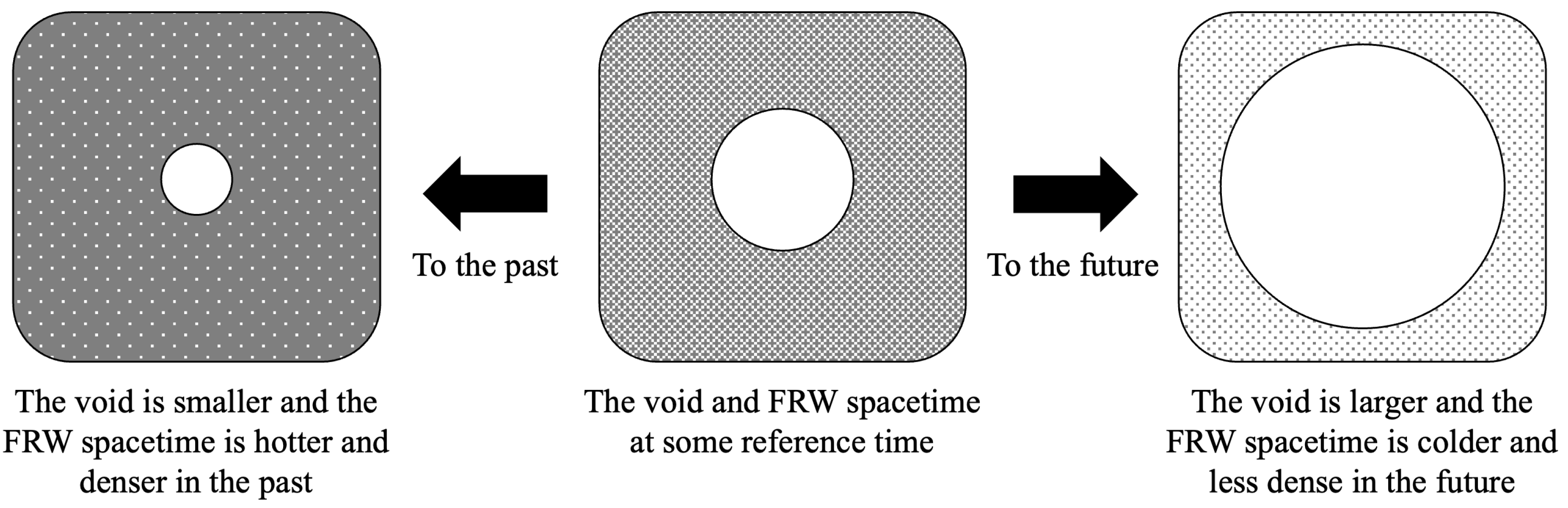
Figure 2.
Kruskal-Szekeres Coordinate Chart
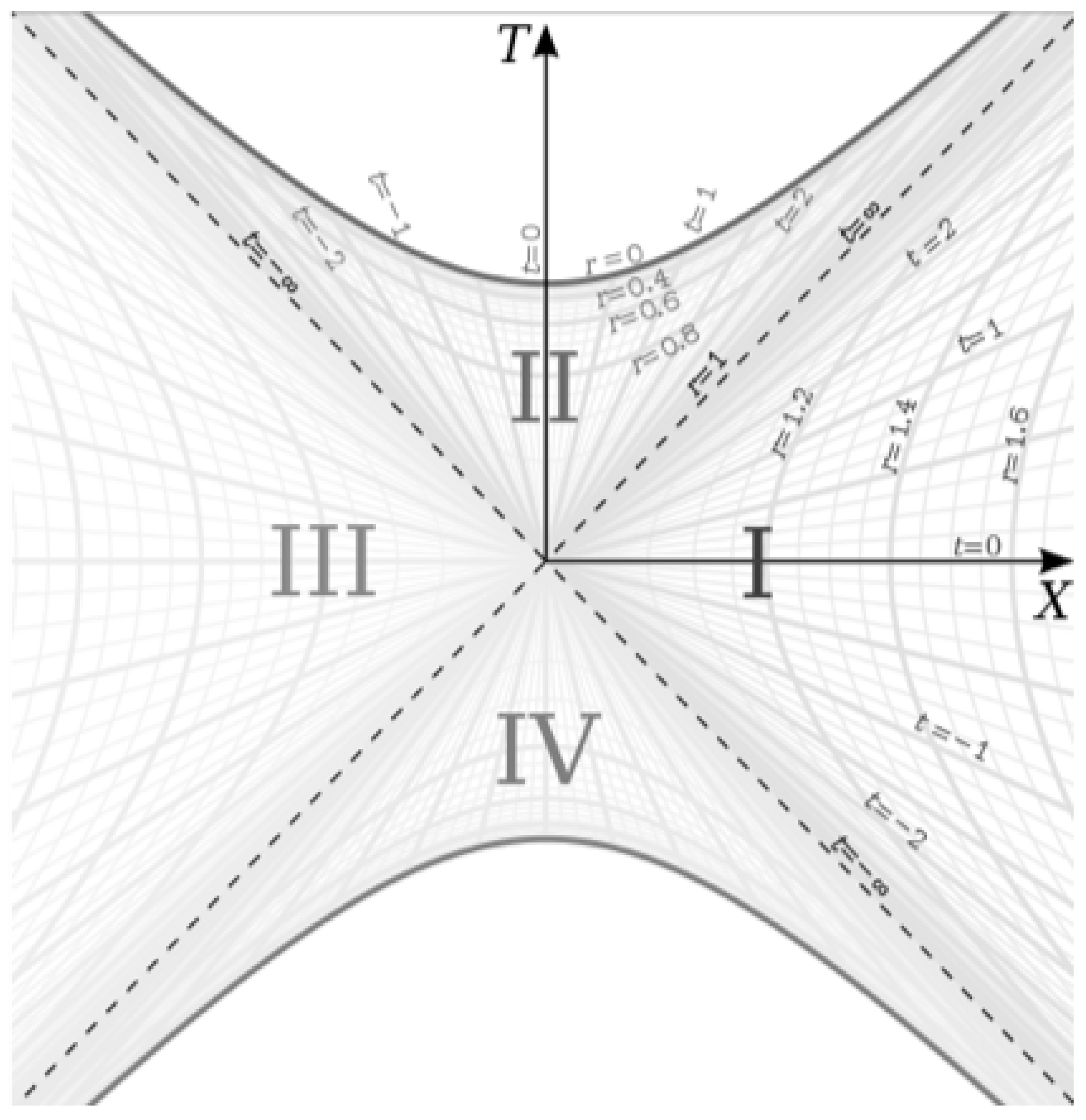
Figure 3.
Surface of Constant for the Exterior Metric in Kruskal-Szekeres Coordinates
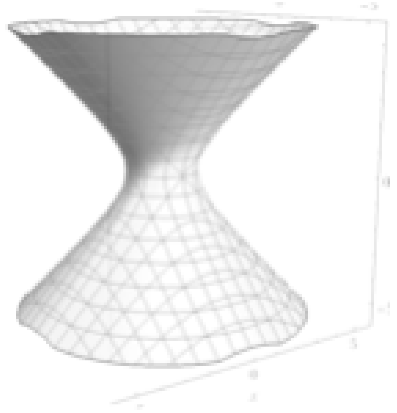
Figure 4.
Surface of Constant for the Interior Metric in Kruskal-Szekeres Coordinates
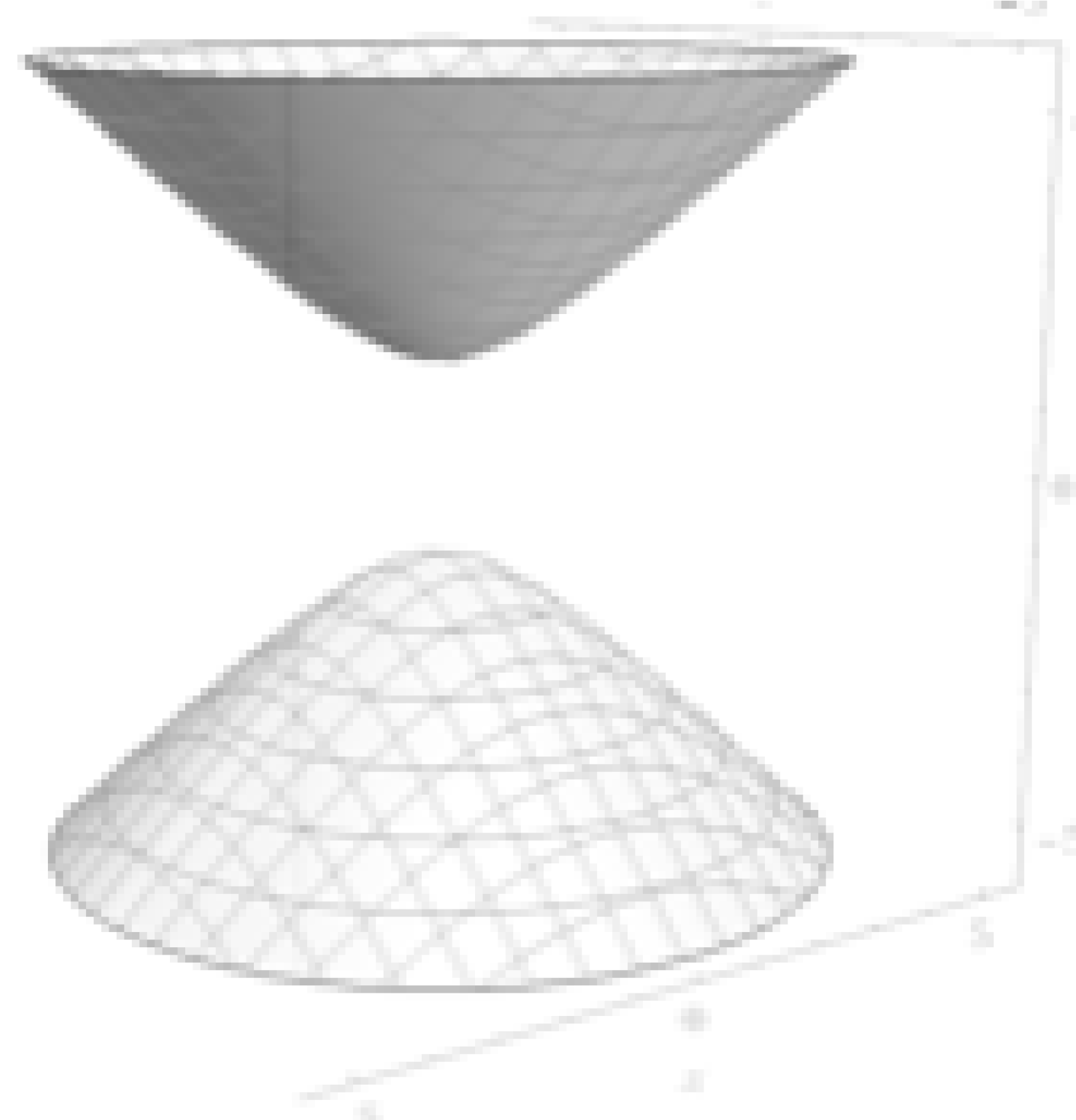
Figure 5.
Parallel Transport of Normal Vectors on a Spherical Surface
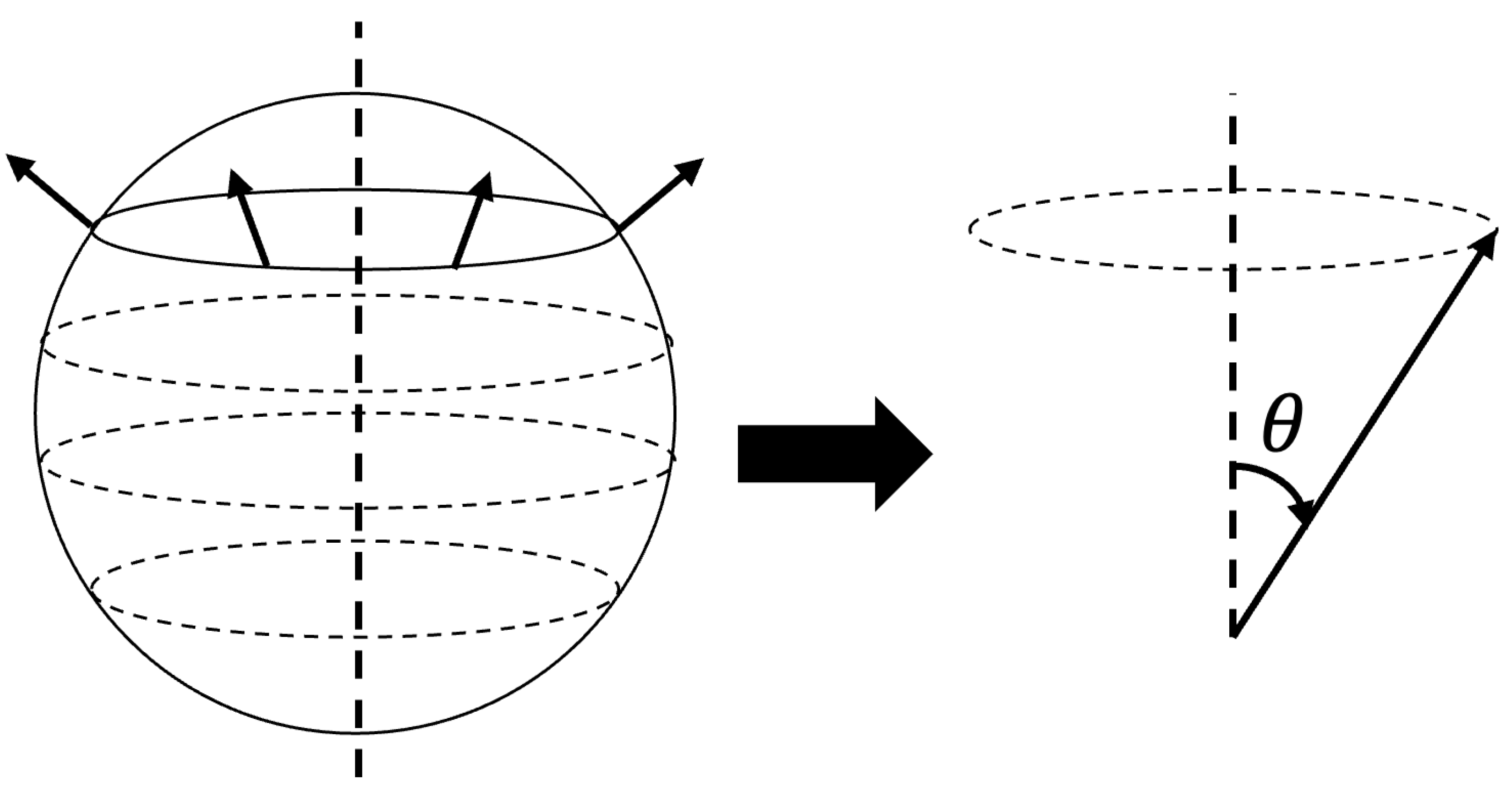
Figure 6.
Parallel Transport of Normal Vectors on a Hyperbolic Surface
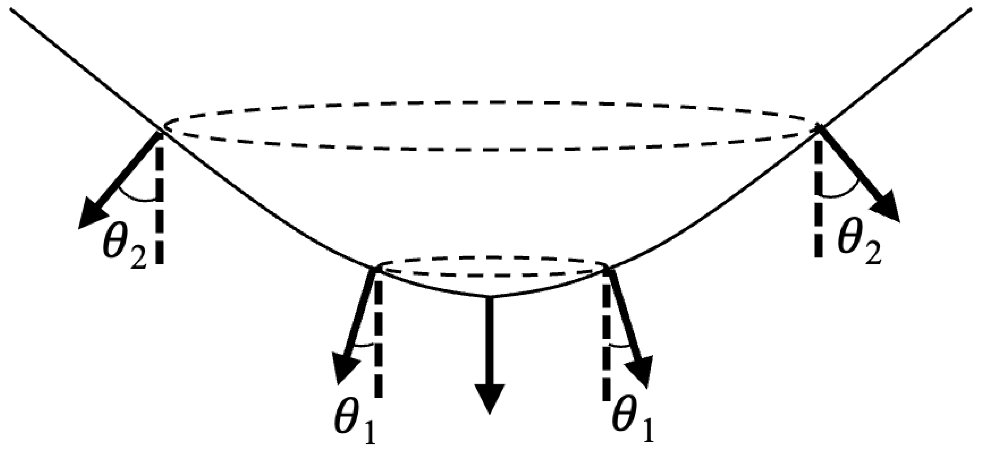
Figure 7.
Viewing a Spacelike Hyperbola from
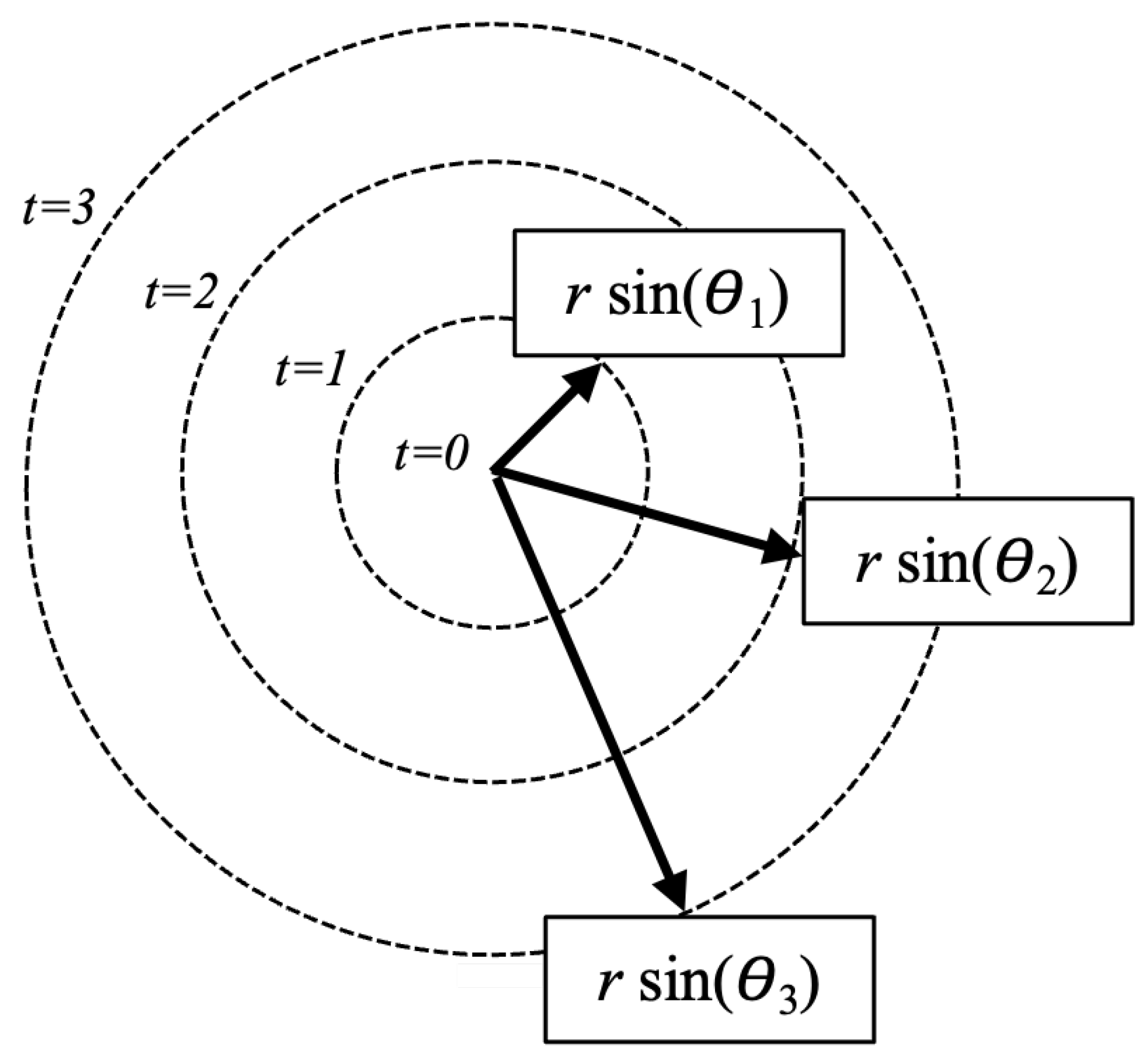
Figure 8.
Radial Lines of the Interior Metric on the Kruskal-Szekeres Coordinate Chart
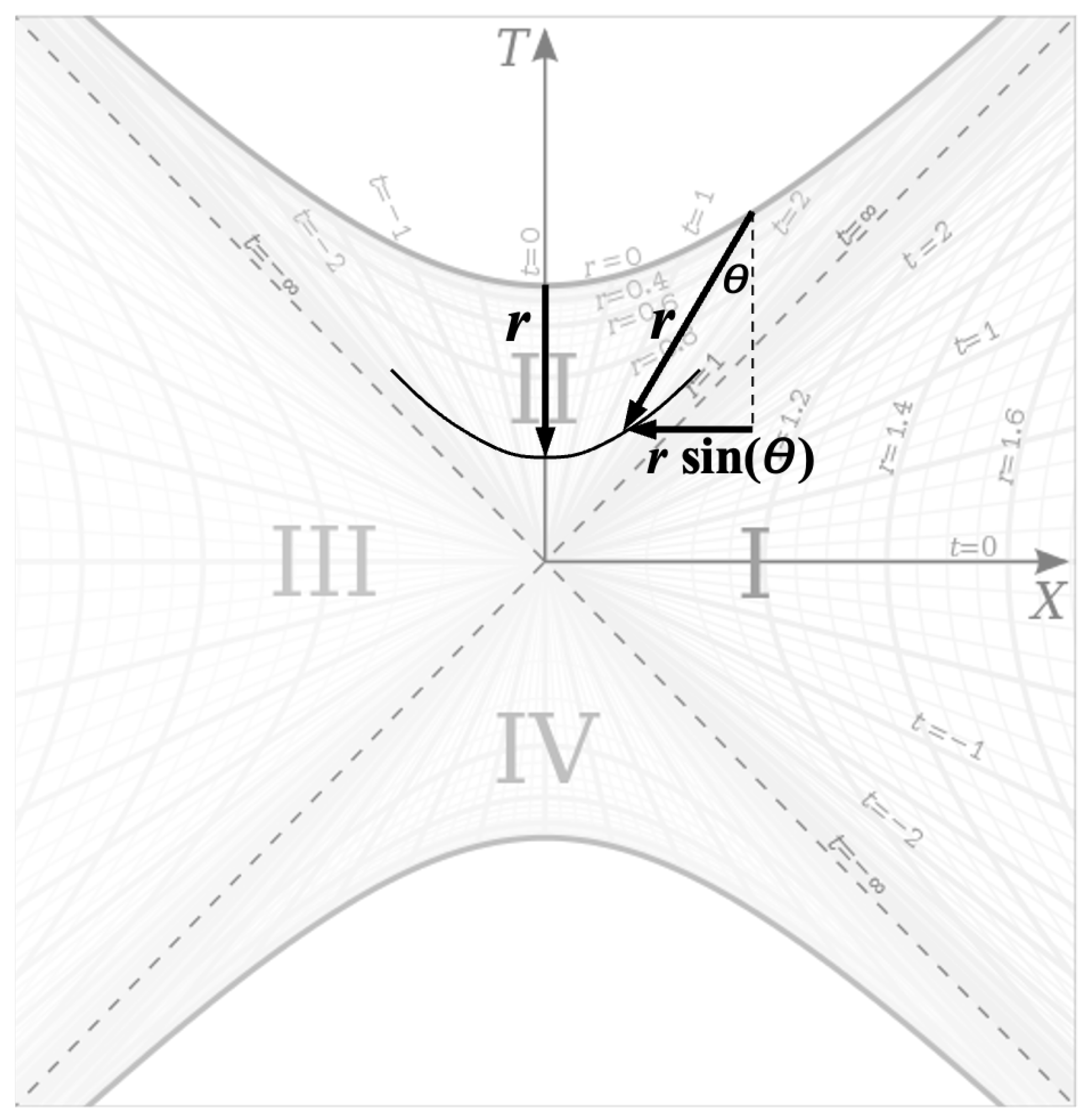
Figure 9.
Lines of Latitude (t) on a Sphere of Constant r
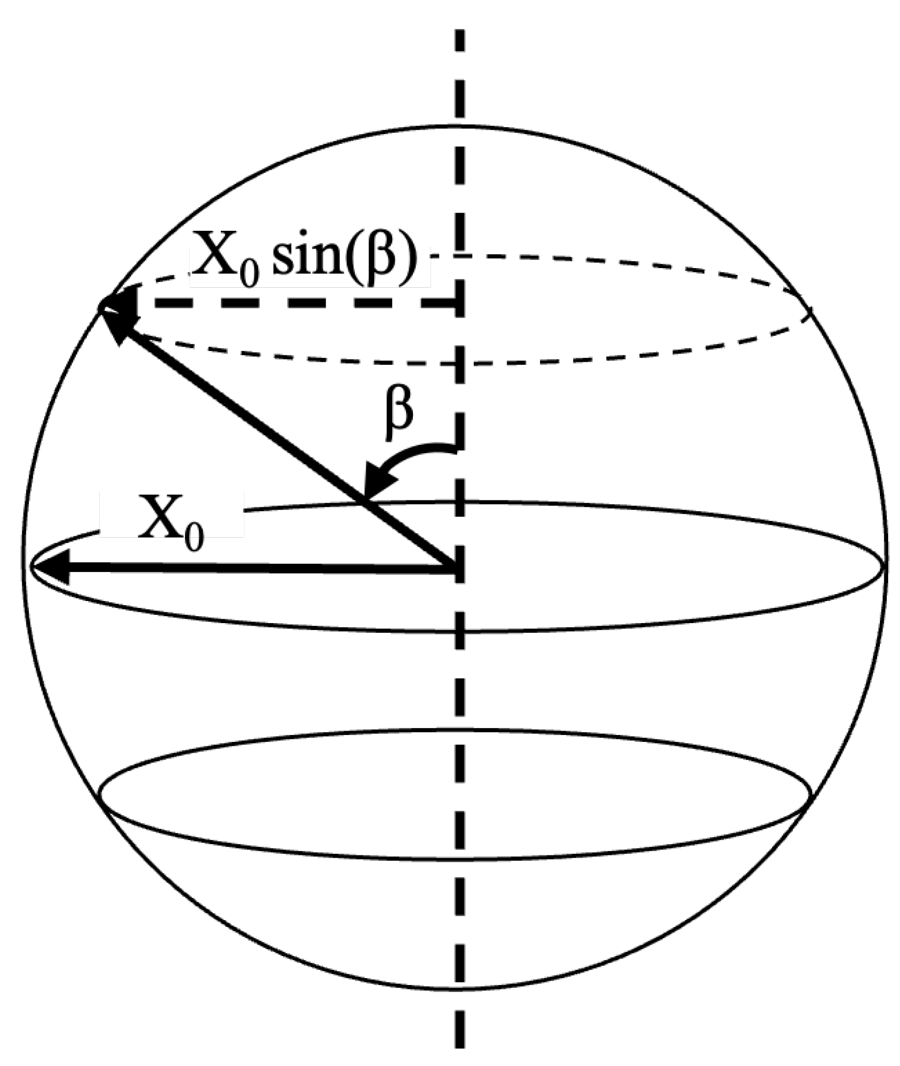
Figure 10.
Lines of Latitude Projected onto a Plane of Constant T
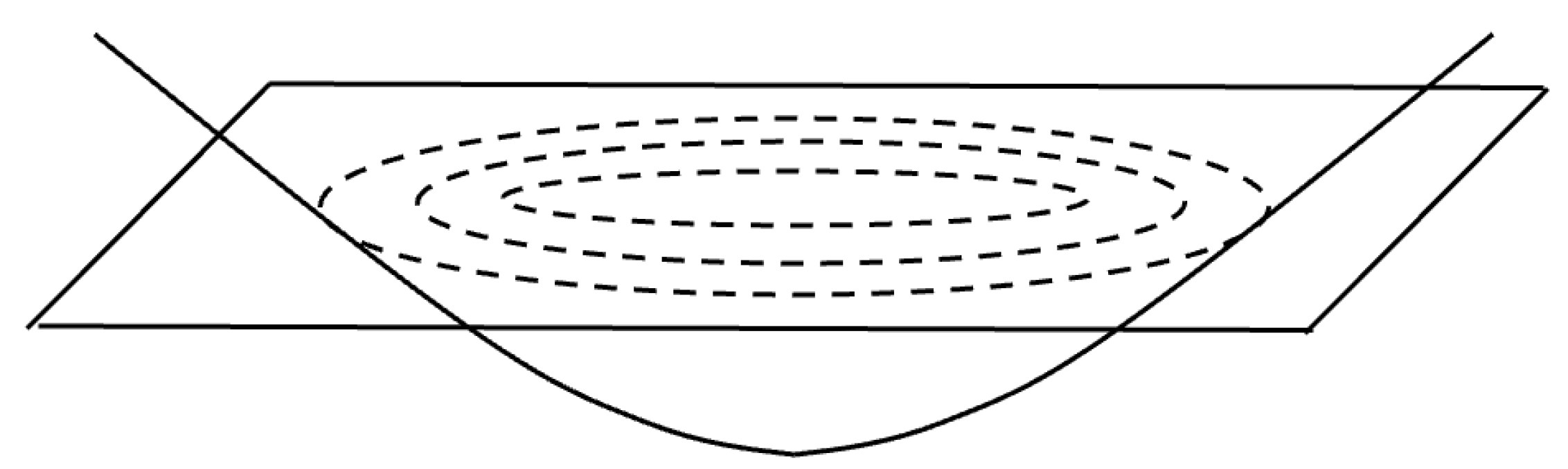
Figure 11.
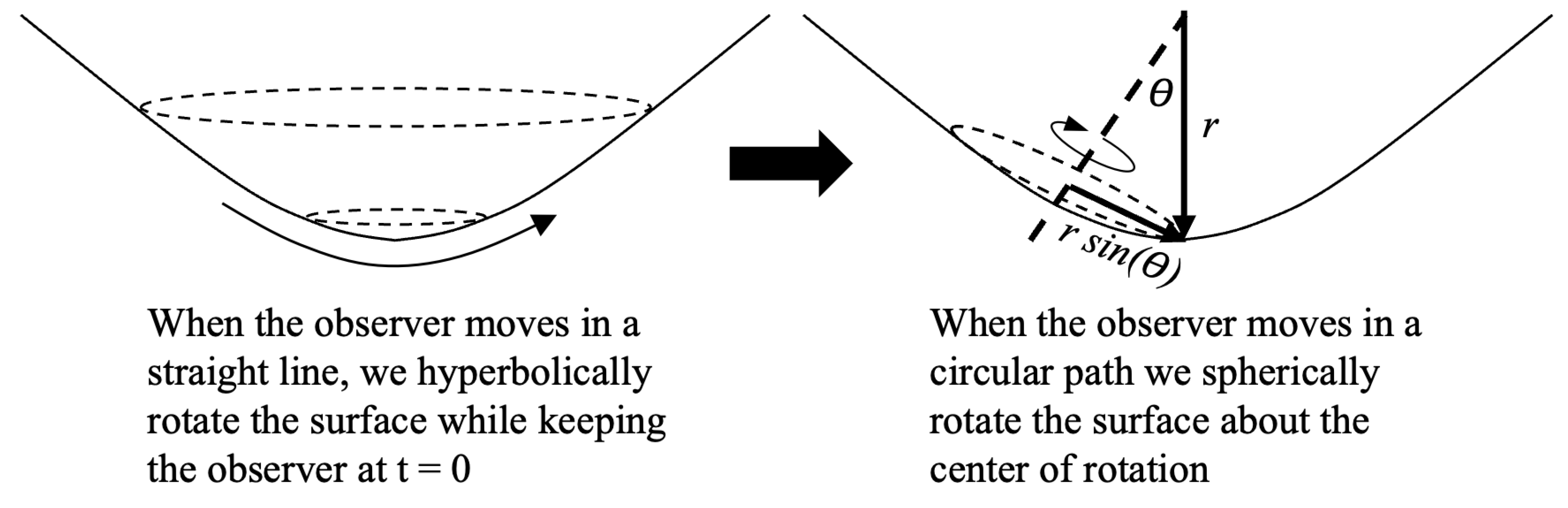
Figure 12.
Reference Frame of a Comoving Observer on the Kruskal-Szekeres Coordinate Chart
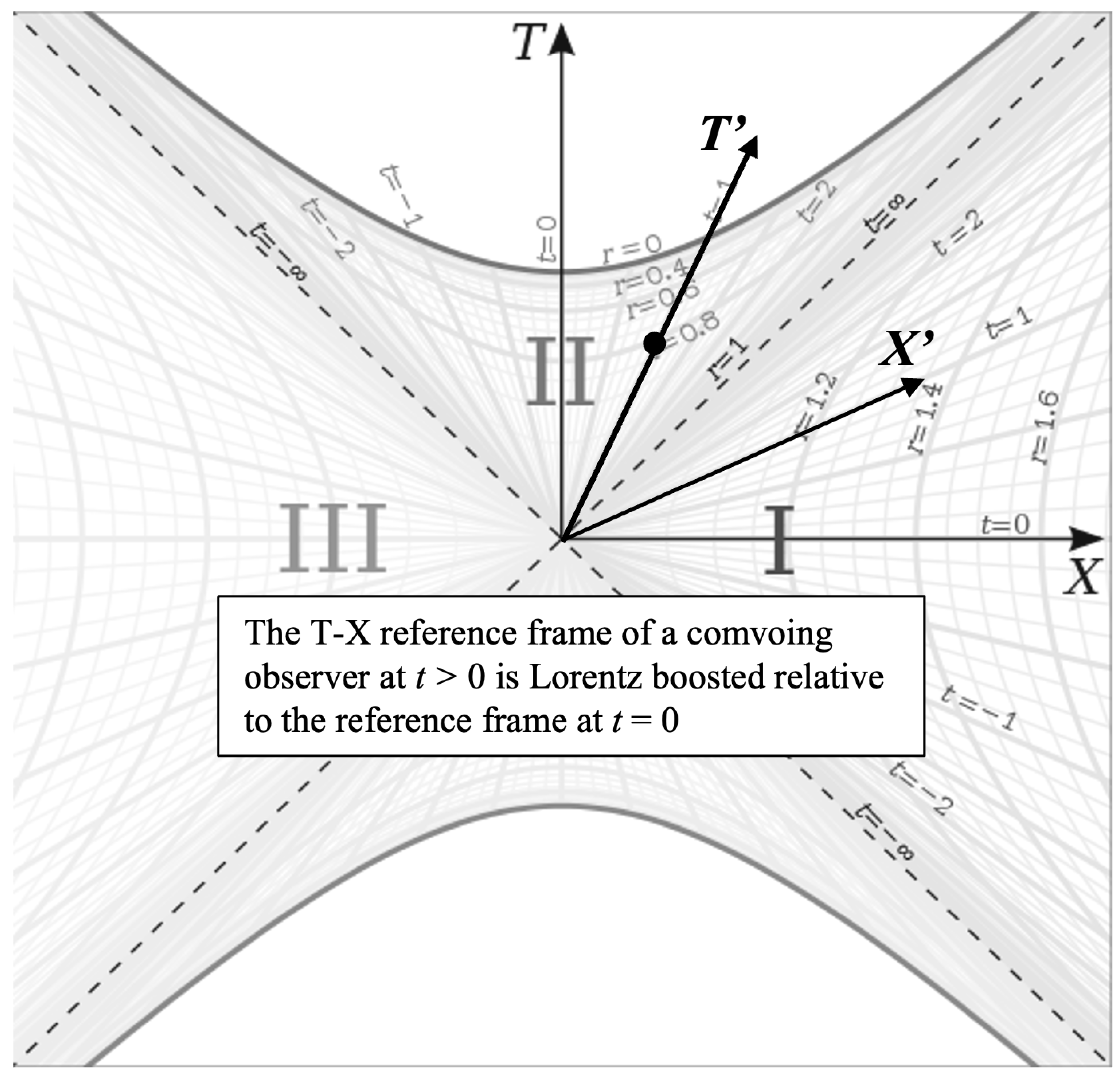
Figure 13.
Velocity Vectors of an Orbiting Observer
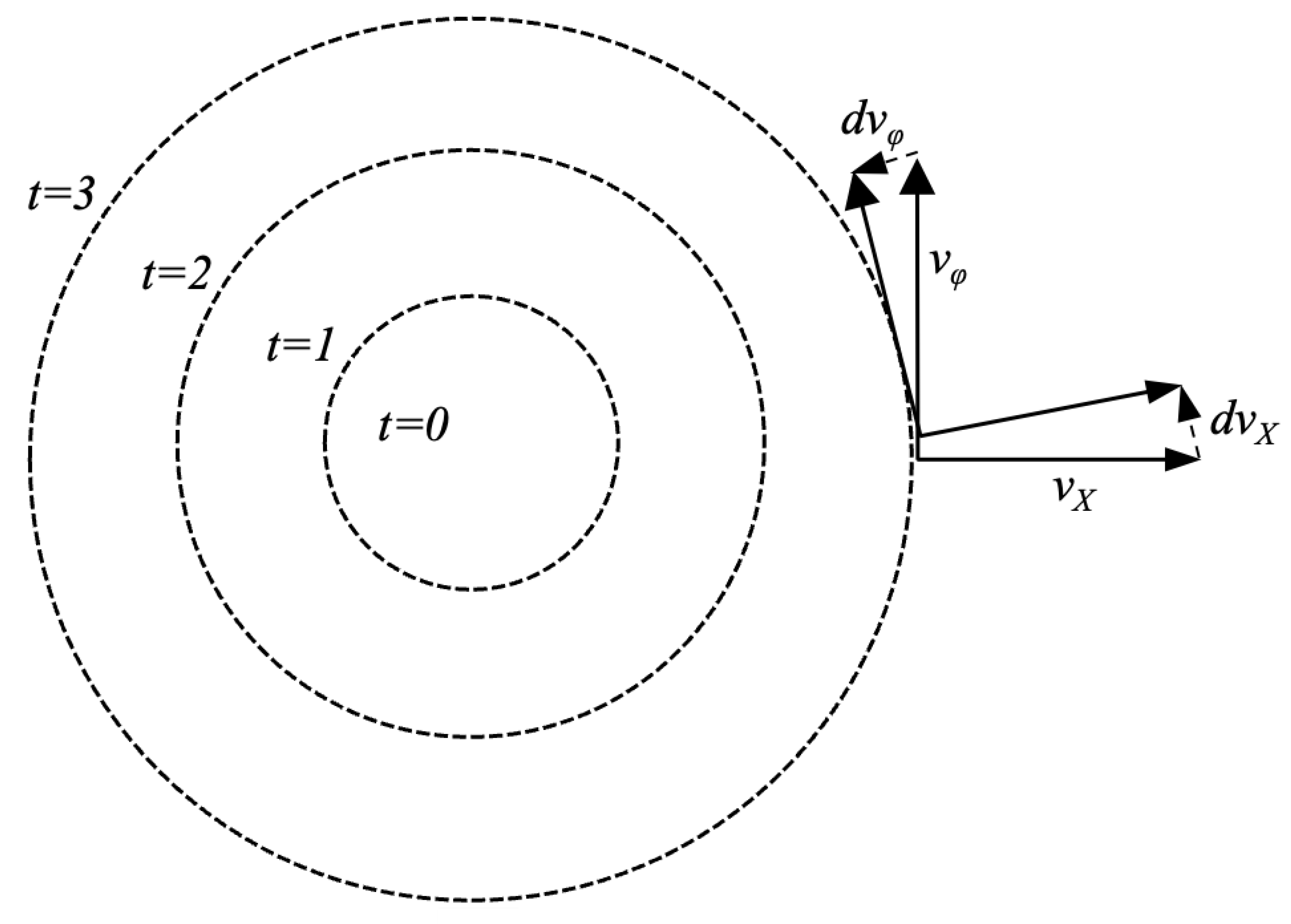
Figure 14.
Lorentz Boost of an Orbiting Observer
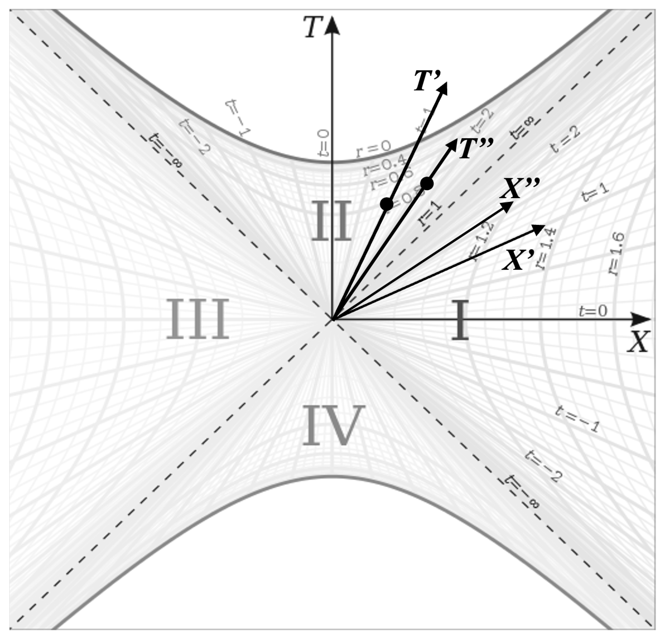
Figure 15.
Scale Factor vs. r for
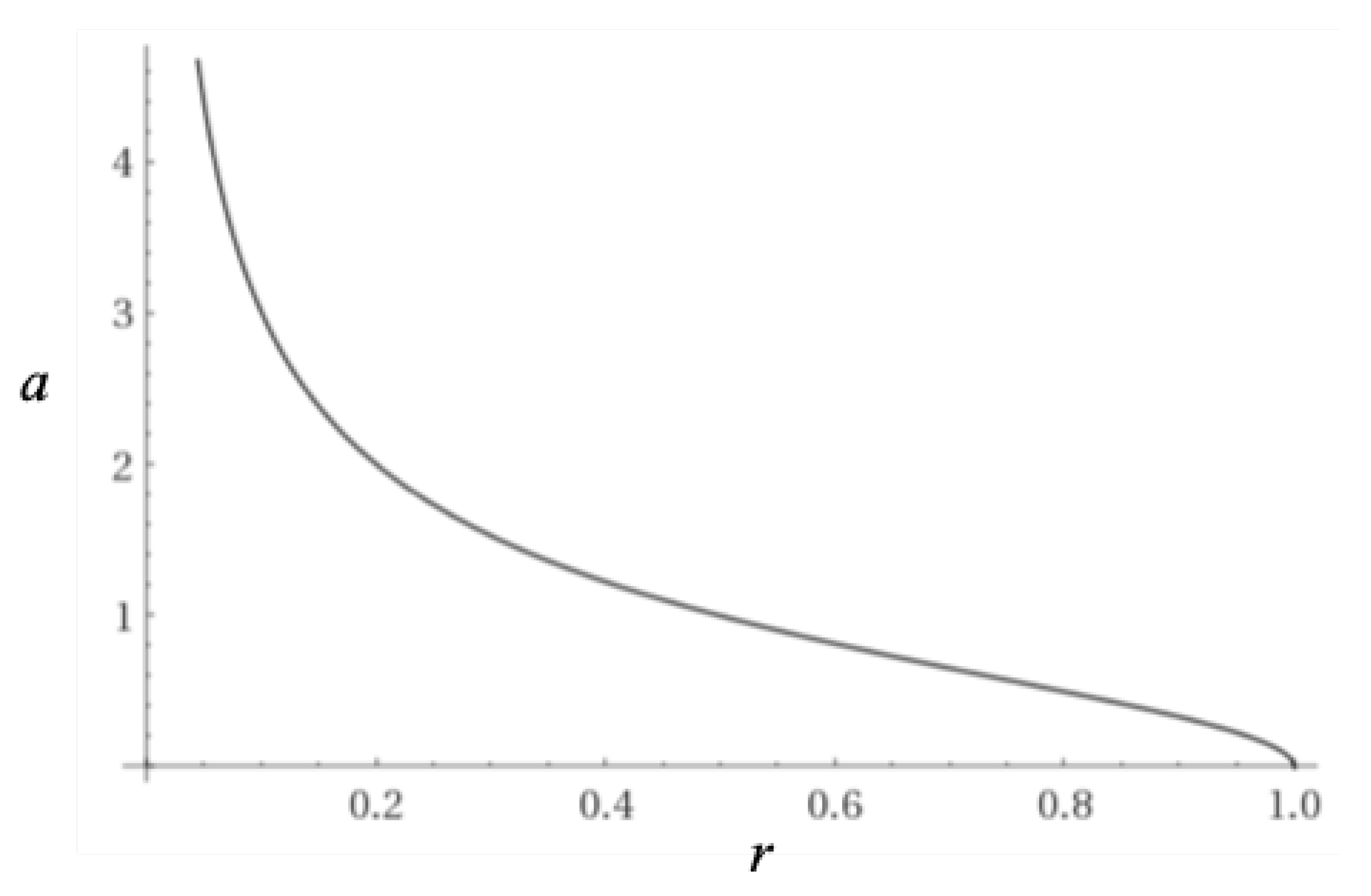
Figure 16.
Distance Modulus vs. Redshift Plotted with Supernova Measurements
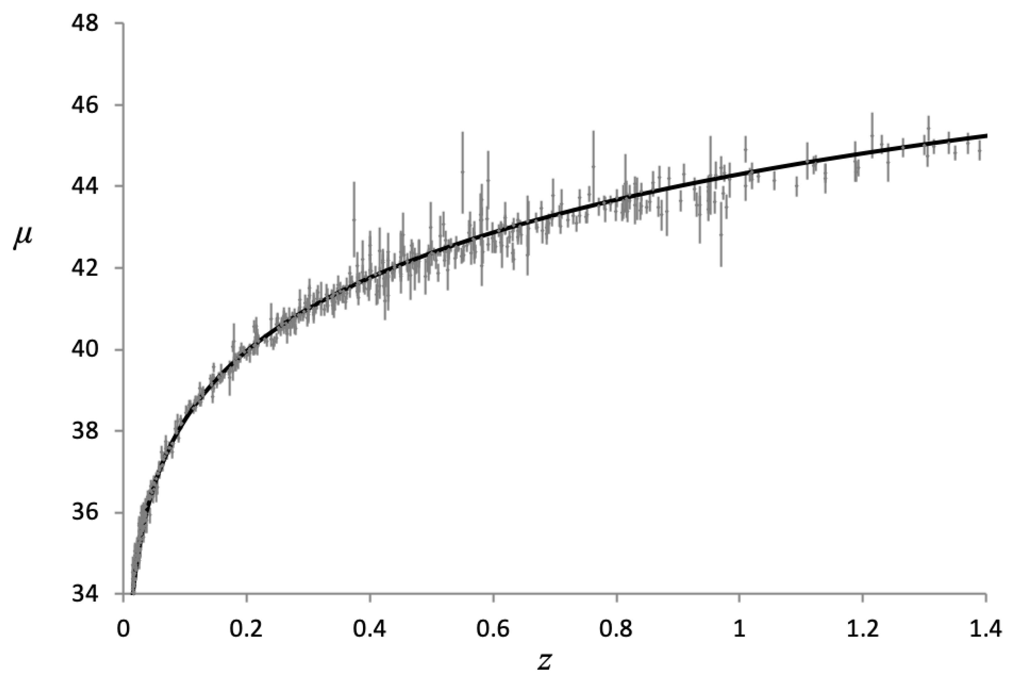
Figure 17.
Distance Modulus vs. Redshift Plotted with Quasar Measurements
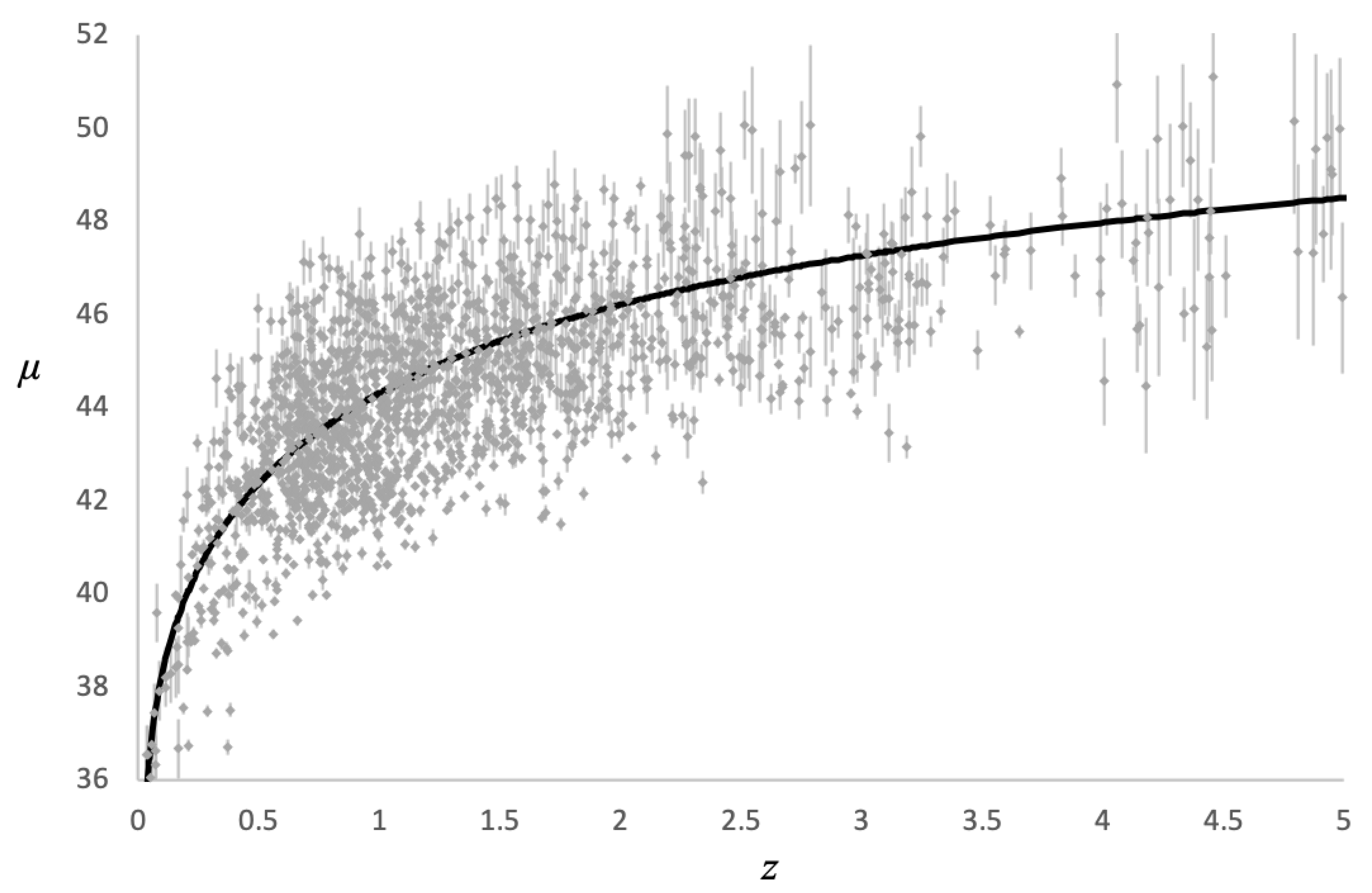
Figure 18.
Distance Modulus vs. Redshift Comparison with CDM
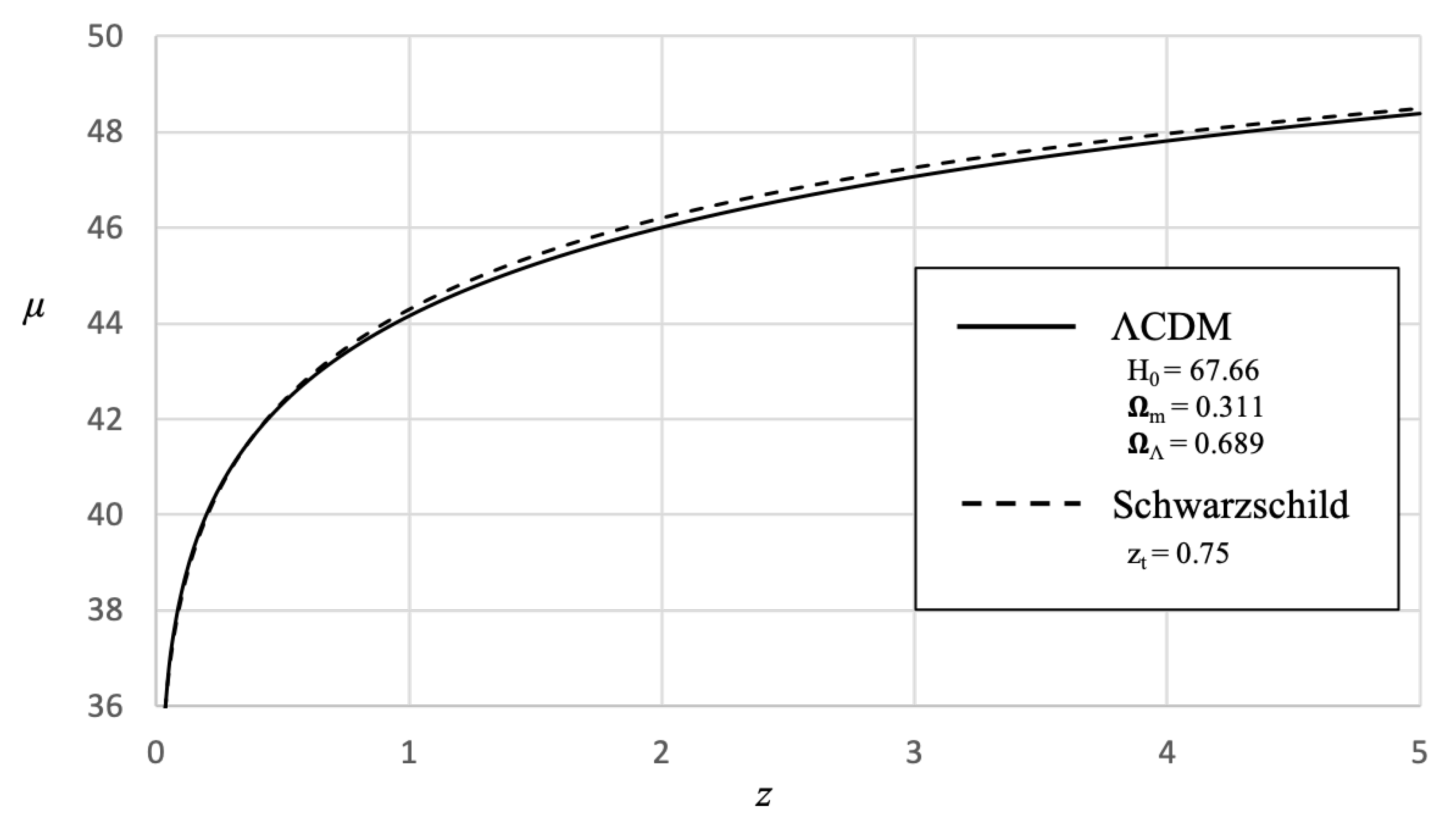
Figure 19.
Lookback Time vs. Redshift
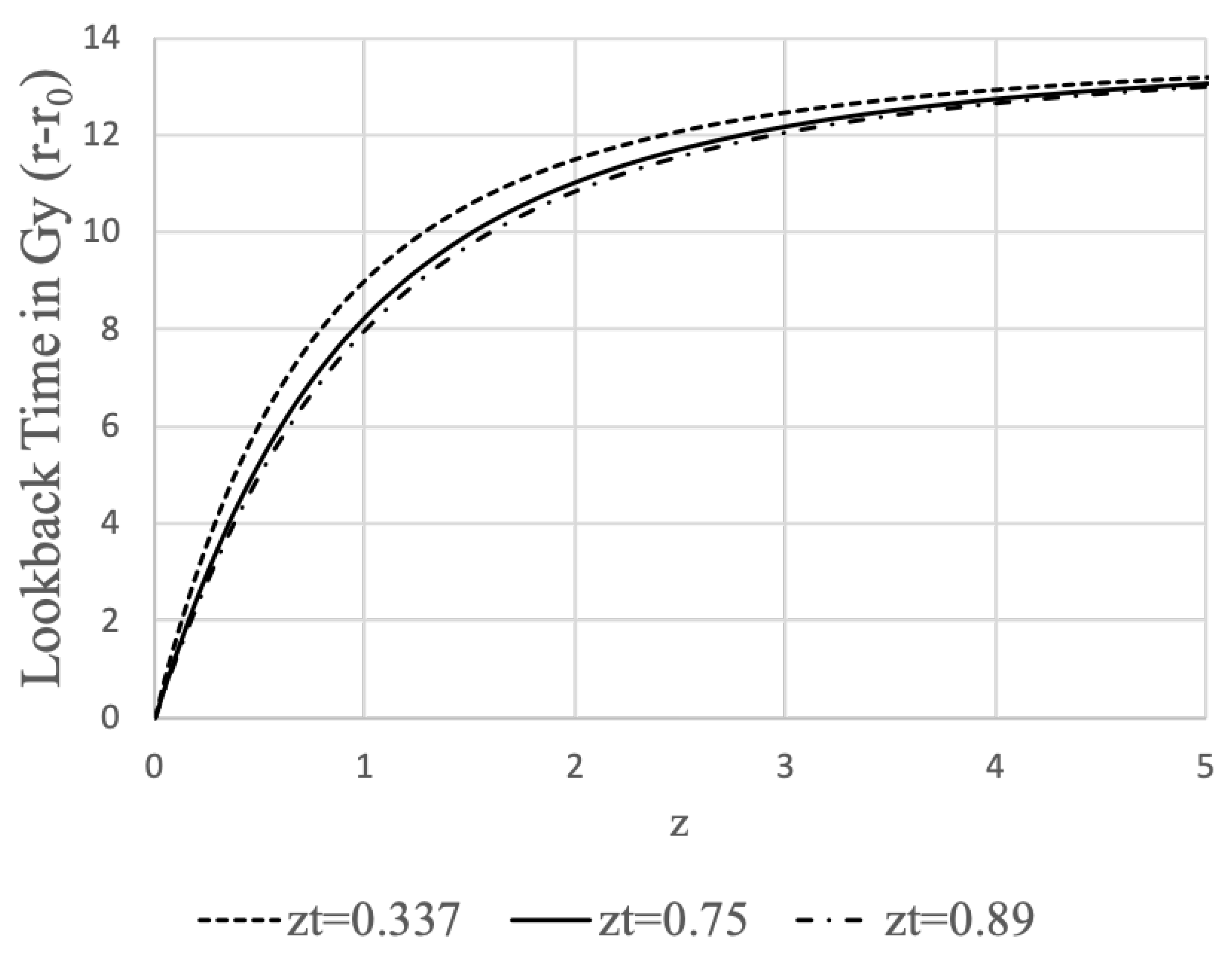
Table 1.
Limiting Cosmological Parameter Values Based on Measurement and a 13.8 Gy Age of the Universe
Table 1.
Limiting Cosmological Parameter Values Based on Measurement and a 13.8 Gy Age of the Universe
| u | ||||||||
| 0.337 | 13.8 | 37.0 | 23.2 | 56.6 | 0.77 | -0.49 | 0.0007 | 0.99 |
| 0.75 | 13.8 | 27.3 | 13.5 | 71.6 | 1.01 | -1.02 | 0.0009 | 0.99 |
| 0.89 | 13.8 | 25.4 | 11.6 | 77.6 | 1.09 | -1.17 | 0.0010 | 0.99 |
Disclaimer/Publisher’s Note: The statements, opinions and data contained in all publications are solely those of the individual author(s) and contributor(s) and not of MDPI and/or the editor(s). MDPI and/or the editor(s) disclaim responsibility for any injury to people or property resulting from any ideas, methods, instructions or products referred to in the content. |
© 2025 by the authors. Licensee MDPI, Basel, Switzerland. This article is an open access article distributed under the terms and conditions of the Creative Commons Attribution (CC BY) license (http://creativecommons.org/licenses/by/4.0/).
Copyright: This open access article is published under a Creative Commons CC BY 4.0 license, which permit the free download, distribution, and reuse, provided that the author and preprint are cited in any reuse.


