Submitted:
11 November 2024
Posted:
11 November 2024
Read the latest preprint version here
Abstract
In this paper, we analyze the geometric and physical implications of the interior Schwarzschild metric, where surfaces of constant \( r \) form a hyperbolic sphere (a 2-sheeted hyperboloid), as opposed to the Euclidean sphere of the exterior metric. By examining this interior metric independently, we show that a comoving observer perceives an isotropic, homogeneous spacetime in its past light cone, consistent with the Cosmological Principle, characterized by concentric celestial spheres foliating the hyperbolic spacetime.Our study reveals that in this hyperbolic geometry, particles in orbit experience an increase in orbital velocity due to geodesic equations, even without a change in the spacelike radius of the orbit, while length contraction explains the orbit’s reduced path length in the particle's frame. We embed a Black Hole in this spacetime, demonstrating that its Schwarzschild radius contracts to a point due to time dilation effects interacting with the hyperbolic geometry.Finally, we propose a cosmological model in which a Universe/Antiverse pair generates an FRW Universe, evolving into a Schwarzschild-like universe. This model is shown to agree with cosmological data and provides a natural explanation for Dark Energy without requiring a cosmological constant.
Keywords:
cosmology
; black holes
; dark energy
; Schwarzschild metric
1. Introduction
In this paper we demonstrate that while in the exterior Schwarzschild metric, a surface of constant r is a Euclidean sphere, a surface of constant r in the interior metric (where r is a time), is a hyperbolic sphere, represented as a 2-sheeted hyperboloid. The consequences of the difference in these two geometries are investigated.
We find that if we consider the interior metric on its own, without reference to the exterior metric (i.e. we consider the spacetime of the interior metric as being a standalone spacetime, not the inside of a particular Black Hole), that the past light cone of a comoving observer in this metric shows the observer an isotropic spacetime that is homogeneous at a given time r. The comoving observer sees concentric celestial spheres which are spherical foliations of the hyperbolic spacetime. This indicates that the interior spacetime would look isotropic and homogeneous in accordance with the Cosmological principle.
We find that due to the hyperbolic geometry of the spacetime, particles in orbit will have their orbital velocities accelerated according the the geodesic equations over time without decreasing their spacelike distance from the center of the orbit. While a comoving observer will see the orbital velocity of the particle increase over time, in the frame of the orbiting particle, the path length of the orbit is reduced due to the length contraction of the hyperbolic surface in that frame. This inertial acceleration is the result of the definition and behavior of the coordinate for the hyperbolic sphere.
We then embed a Black Hole inside this spacetime and show that while a Black Hole placed in Minkowski spacetime would have an interior region, in this hyperbolic spacetime, the Schwarzschild radius contracts to a point as a result of how the infinite time dilation at the horizon interacts with the underlying hyperbolic geometry.
We present a model of cosmology where the intersection of a Universe/Antiverse pair (a consequence of the spacetime being a 2-sheeted hyperboloid) generates an FRW Universe and Antiverse. This FRW Universe subsequently cools and expands, transitioning into a Schwarzschild Universe as the matter clumps and spherically symmetric vacuua emerge between the regions of concentrated matter. This model is compared to cosmological data and it is found that it is capable of accounting for the Dark Energy of the Universe without the need for a cosmological constant.
2. Analysis of the Geometry of the Interior Metric
The Schwarzschild metric has the following form:
The exterior metric, which describes the spacetime around a spherically symmetric mass is given for values of where u is the Schwarzschild radius related to the mass M of the source given by . This metric treats the mass of the source as being concentrated at point at the center of the spacetime.
The interior metric is known as a ’Kantowski-Sachs’ spacetime which has different linear and azimuthal scale factors. This is understood to mean that the spacetime is anisotropic [1]. Figure 1 shows a common depiction of the gravitational well of the Schwarzschild metric (, ).
We are given the impression here that the geometry inside and outside the event horizon are the same with the main difference being that once an observer crosses the event horizon (), they will continue to fall to the singularity at where they will be ’spaghettified’ as a result of the radius of the 2-sphere collapsing to a point and the t dimension becoming infinitely stretched.
Since r is spacelike in the exterior metric, at constant r space is a 2-dimensional spherical surface. But in the interior metric, a surface of constant r is a 3-dimensional spacelike volume. As will be shown, space in the interior metric is hyperboloidal, in particular it is a hyperbolic sphere and therefore the space inside the Black Hole is very different than space outside and we seek to fully understand the geometry of the interior metric.
So we need to examine the exterior and interior geometries more closely to understand how exactly they are different, particularly in regards to the meaning of the azimuthal term in each case. The Kruskal-Szekeres coordinates are very useful for this task. As we will see, the Kruskal-Szekeres coordinate chart allows us to see how the t and r coordinates are curved relative to Minkowski space. But first, we define the Kruskal-Szekeres coordinates in terms of the Schwarzschild coordinates. For the exterior metric:
And for the interior metric:
With these definitions, we can plot the Kruskal-Szekeres coordinate chart [2]:
Figure 2.
Kruskal-Szekeres Coordinate Chart.
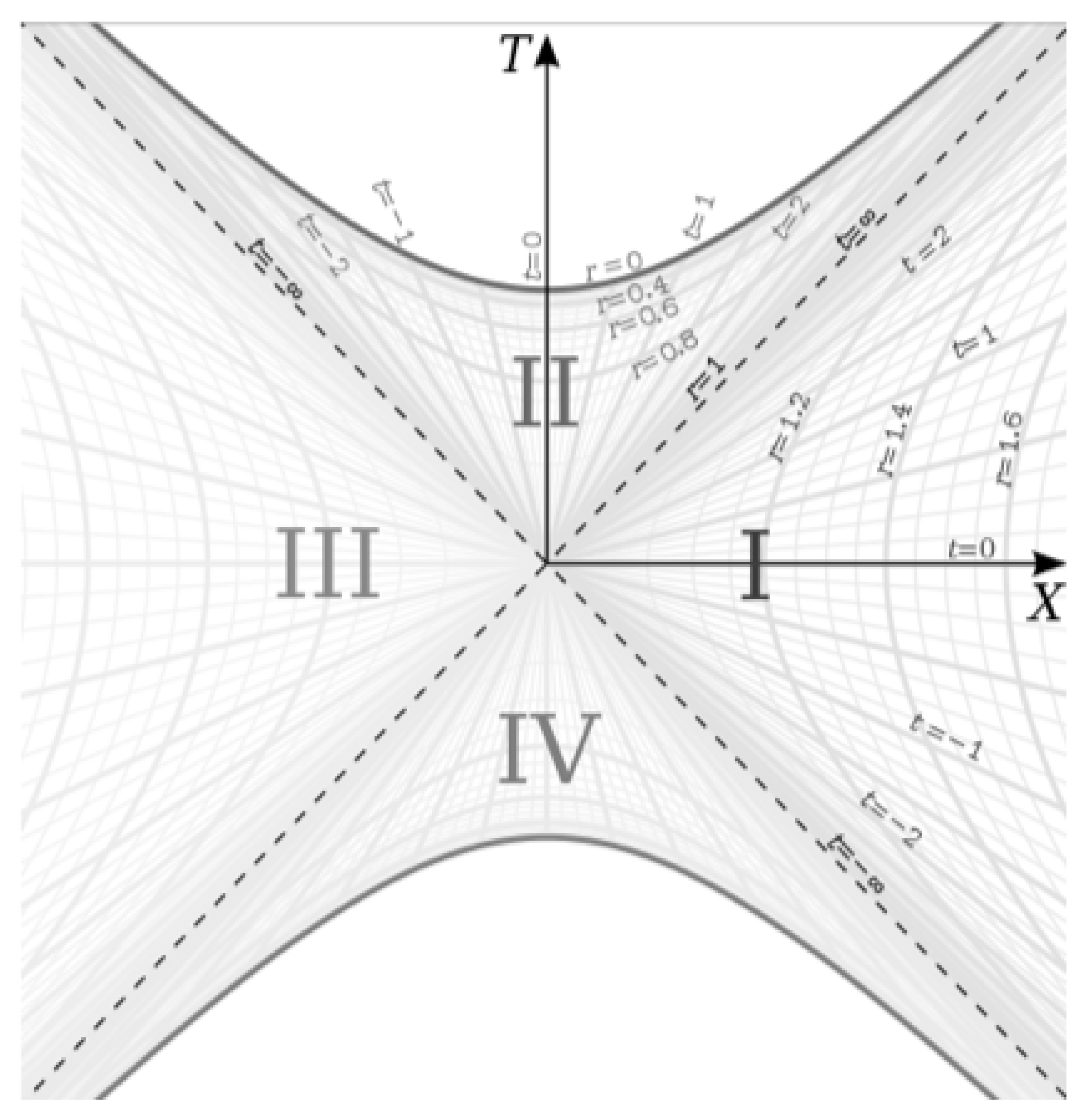
In this paper, we will focus primarily on regions I and II of this chart, representing the exterior and interior metrics respectively. Since the Kruskal-Szekeres coordinates are defined in such a way that null geodesics are 45 degree lines everywhere on the chart and the T and X coordinates are straight and mutually perpendicular everywhere on the chart, we can think of the T-X grid as Minkowski space with the curved r and t coordinates overlaid on the grid. Thus, this chart clearly shows how the Schwarzschild space and time coordinates r and t are curved relative to the Minkowski coordinates T and X. We see that the r coordinate lines are hyperbolas, which captures that fact that an observer at rest in the exterior metric experiences a constant acceleration, and the t coordinate is a hyperbolic angle. That t is a hyperbolic angle will become an important fact when we look at the geometry of the interior metric.
We see from Equations (2) and (3) that we need separate Kruskal-Szekeres coordinate definitions for the exterior and interior metrics, but we can combine these into a single relationship as follows
Equation (4) is applicable to both the interior and exterior solutions. For the exterior metric, and for the interior solution, .
The equation for a 2D hyperboloid surface embedded in three dimensions is given by:
For our purposes, we will be considering the special case where , which gives the one and two sheeted hyperboloids of revolution. Equation (4) appears to be only for one dimension of space, but if we think of X as a radius, then it can describe 3 sphrically symmetric dimensions of space.
So comparing to Equation (5), if we set and where R is a radius of a circle in this example, we obtain an equation that matches the form of Equation (5) where :
Equation (6) describes 2D hyperboloid surfaces for a given r where the interior metric has negative and the exterior metric has positive . Let us now visualize a surface of constant r in both the exterior and interior metrics. For the exterior metric at some , we get the following hyperbolid of revolution:
On this hyperboloid, the time coordinate t is marked as circles on the sheet and we have one free spatial coordinate on the surface which is the angle of revolution of the surface. The location is at the throat of the hyperboloid. The first thing to note here is that the t coordinate can only be hyperbolically rotated in one direction: up or down. This is because the t coordinate is the coordinate of time and time only has one dimension so there can only be a hyperbolic rotation along the single time dimension. The second thing to notice is that the radius of the sheet is pointed perpendicular to the axis of circular rotation.
So we can see how if in Figure 3, r was timelike and t was spacelike, as is the case in the interior metric, then the spacetime would be anisotropic because in that case, the entire surface is spacelike and the spacetime looks different in different directions. In one direction, the space is closed (moving around a circle on the hyperbolid as r, which is the time coordinate in the internal metric, decreases), and in the perpendicular direction, the space is open (moving up or down on the hyperboloid).
So if a 2D foliation of the interior metric at some r was represented by the one-sheeted hyperboloid of revolution (like the exterior metric is), then the common visualization of the gravitational well in Figure 1 would be correct. However, we need to recall that for the interior metric, the right side of Equation (4) is negative, which gives the following hyperboloid surface for some constant :
The first thing we notice is that this is a two-sheeted hyperboloid, which is known as a hyperbolic sphere, as opposed to the one-sheeted hyperboloid of the exterior metric. So right away, we can see that the interior and exterior geometries are different.
If we look at region II of Figure 2 in the context of Figure 4, we see that in contrast to the exterior metric where the radius is perpendicular to the axis of circular rotation, in the interior metric, the radius is parallel to this axis. Recall that r is now the time coordinate and time is one dimensional, so the radial vector in this case is stuck in one dimension. Furthermore, we see that the t coordinate, which is a hyperbolic angle, can be rotated in 3 different dimensions now since the t coordinate is spacelike (we see two of the three dimensions in Figure 4). Since t is a hyperbolic rotation and is a Killing vector of the spacetime, we can hyperbolically rotate the space to move any point on the surface to which is at the apex of the hyperboloid. So just like we can set any arbitrary time as in the exterior metric, we can set any arbitrary location as in the interior metric. In particular, for a given comoving frame we are examining, we can say that that comoving frame is always at , and when the frame moves in a straight line (along a hyperbola) in a particular direction, that is modeled as the hyperboloid being hyperbolically rotated in that direction such that the reference frame remains at as it moves.
Therefore, the t coordinate, which is a hyperbolic angle, is like a ’forward/backward’ coordinate. It represents the straight-line distance from the reference frame to some point. In the exterior metric, the hyperbolic rotation could only happen along one direction (the direction of time), but being spacelike in the interior metric, the hyperbolic rotation can now happen in any direction in three dimensions of space.
This brings us to the azimuthal term of the interior metric. Consider Figure 5 which depicts the parallel transport of a normal vector of a spherical surface around a line of latitude of the sphere.
On the left side of the Figure, we see the normal vector being parallel transported and on the right, we see how that vector precesses as it is transported. So for the exterior metric at some r, the precession of the normal vector as it is transported around the loop gives us the and values of the path that are used in the metric. The important thing to note here is that will increase or decrease as the path moves toward or away from the to pole of the sphere.
In the interior metric, space is hyperboloidal, but we can use the same technique transporting a normal vector around one of the sheets (the top sheet in this analysis) to help us understand the angular term of the interior metric. Figure 6 shows how and are defined for the interior metric.
As was the case for the sphere, is the angle of revolution of the transported normal around the central axis while is the angle of the normal relative to vertical. So at , and increases as we move away from . One thing making the hyperbolic geometry different than the spherical geometry is that as , in the interior metric. This means that while on the sphere of the exterior metric, , in the (unaltered)) interior metric, .
Since the surface in Figure 4 is at constant r, which is a time, we see that and in particular acts like a spatial radius, giving the spacelike circles on the surface different circumferences even though they are all at the same radius.
Let us us calculate the proper circumference of one of these circles. The circle has and noting that in Equation (1), the proper circumference will be given by:
We can relate of a given circle to t in this context by noting that the slope of the surface tangent is given by . The angle between the tangent vector and vertical will be equal to the angle between the normal and the vertical and is given by:
And so we can calculate the value of from t. Next, let’s consider motion around one of these circles. In this case, along the path. The geodesic equations for and are given below [3] where we use as the affine parameter.
Since we are moving on the circle, the initial condition is that . We see from Equation (9) that even though we start with a constant , there will still be a change in over time since is not zero.
So what is of interest here is that is changing over time even though the initial was constant. This suggests the particle is changing its distance from the point along the hyperbola. However, still remains constant because the angular geodesic equations are not functions of t, nor is the geodesic equation of t a function of or :
In this case, in the observer’s frame, the circles must be decreasing or increasing in size (depending on the sign of ) over time. The value of t remains constant at all times, so this suggests that the cause of the increase in must be due to a length contraction relative to the coordinates that makes the slope of the surface at the observer’s location t more parallel to the T axis (if the slope is parallel to T, then ).
Let us consider Figure 7 which shows a projection of the velocity 4-vector of an orbiting observer on the Kruskal-Szekeres coordinate chart.
We see two components of the 4-vector in this figure, but there is also a 3rd component pointing into the page (the tangential velocity). What we see is that since is by definition zero for the orbiting observer, as time passes, the worldline follows the line of constant t that the observer is on. We therefore see in Figure 7 that the tilt of the t coordinate line results in a relative velocity of the orbiting observer relative to the frame in the X direction (meaning there will be length contraction in the X direction). This projection is coming from the timelike component of the 4-velocity. We also note that the angle of the velocity vector relative to the T axis is also equal to . This does not happen in Special Relativity because the spacelike coordinate lines are parallel to the time axis everywhere in Minkowski spacetime, so there would be no such projection.
So this projection will cause a Lorentz boost of the orbiting frame relative to the frame as shown in Figure 8.
On the left, we see the tangent to the surface of a co-moving observer at some location t. When that observer is orbiting, the projection of its 4-velocity onto the X axis causes a Lorentz boost in the coordinates as shown on the right. In this frame, the boost moves the observer outward on the diagram along the hyperbola as the velocity increases. Since is zero, it is the t coordinate lines whose angles are changing that move the points along the hyperbola (so the angle of some t in the comoving frame is smaller than the angle of the same t in the boosted frame). And we can see that as the speed tends toward the speed of light, the angle between the surface at the observer’s location in the boosted frame becomes parallel to and therefore, the angle becomes there (and since the largest possible in the comoving frame is , we see that the boost will increase the angle regardless of the orbit size.
The metric in Kruskal-Szekeres coordinates is given by:
If we solve for at some r we get:
Where and are functions of the projections of the 4-velocity shown in Figure 7.
Next we consider the past light cone of a comoving observer at stretching back to the horizon. Each hyperboloid the cone intersects looks like a celestial sphere to the comoving observer. In Figure 4, a light cone intersecting the hyperboloid would make a circle on the hyperboloid. But that hyperboloid represents only 2 of the 3 dimensions of space. The third dimension comes from the fact that each of those circles actually represents a 2-sphere since the metric is spherically symmetric. So in the frame of the comoving observer, that observer is at the center of a continuum of isotropic celestial spheres where larger and larger spheres are 2D foliations of space at earlier and earlier times.
We can derive the expression for t vs. r along a null geodesic where the geodesic ends at the current time and by setting in Equation (1) and integrating:
Thus, if we know at which time r a given sphere is, we can calculate t for that sphere and use Equations (7) and (8) to calculate proper distances on the sphere.
So we are beginning to see that the interior metric is looking a lot like what we observe in cosmology. To the comoving observer, space at a given time is homogeneous and their past light cones show an isotropic spacetime. Next let’s examine what happens when we place a Bleck Hole in this spacetime.
3. A Finite Black Hole Inside an Infinite Black Hole
A black hole embedded in the interior metric is still a spherically symmetric vacuum and is therefore still a valid application of the Schwarzschild spacetime. What we want to know is how does a Black Hole at some fixed time change the spacelike hyperboloidal surface of the interior metric, which itself is a spacelike surface at some fixed time.
First, lets imagine how a surface of constant time t in Minkowski space would be affected by a Black Hole with radius 1.
In Figure 9, we can think of the vertical coordinate as the proper time of rest observers. The black line is a line of constant t, which is the time coordinate of the infinite observer. The curve asymptotes to as . We see that at the horizon, because time dilation is infinite there and so no matter what the value of t is, will always be zero. As we move away from the horizon, the ratio increases until it is 1 at infinity.
This line is a plot of the time dilation of the rest observer in the exterior metric:
Where in this case. So in Minkowski space without a Black Hole, the t coordinate line is flat. But when we put the Black Hole in the spacetime, we multiply each point on the line by the time dilation of the rest observer at that point and we see how the spacelike surfaces in Minkowski spacetime are deformed by the Black hole. Furthermore, the slope of the line in Figure 9 at a point is also the gravitational acceleration at that point given that:
Which is recognizable as the proper acceleration of a rest observer in the exterior Schwarzschild metric.
So to embed the Black Hole in the interior metric, we follow a similar process. Consider Figure 10.
At the top left, we show the typical visualization of a gravitational well up to the event horizon. To the right, we show the pairs of points representing each circle drawn on the well where the two innermost points represent the event horizon. Note that each pair of points corresponds to a value of t in the interior metric because t is the spacelike coordinate in this metric. Therefore, if we assume a Schwarzschild radius of 1, the two innermost points are at .
We deform the surface on the top right of Figure 10 one point at a time by first hyperbolically rotating the point to . We then scale the value of that point by multiplying it by the time dilation of the rest observer at that point. We then hyperbolically rotate that shifted point back to its initial t coordinate. Therefore, we can find the new T and X coordinates for a given point as follows:
Where and T and X are the original T and X coordinates. Figure 11 shows a plot of the surface with and with the undeformed surface shown as a dashed line for reference:
What is most striking about this construction is that in this hyperbolic spacetime, the event horizon is shrunk to a point. So in this spacetime, there is no interior metric inside the Black Hole, the horizon contracts to a point as it is approached and we end at the horizon at .
If we think about orbiting bodies in the exterior metric, a body that has a that is greater or smaller than , the geodesic equations will cause the body to tend towards an angle of and then the orbit becomes stable and stops changing. So given Figure 11 and our discussion of being the angle between the normal of the surface and the vertical, we see that when we have a gravitational well in this spacetime, increasing to means that in the frame of the orbiting observer, they will move down the well toward the horizon because at the horizon, is closest to . And since this acceleration is infinite as , we can see that objects stably orbiting a Black Hole in this metric will get pulled to the horizon as . So if we imagine a galaxy in this metric, it would act as a drain into which everything orbiting it will fall as .
If we consider systems with small distances and timescales relative to u and t, we see that the vacuum spacetime of that region is approximately flat because that is the region close to the apex of the hyperboloid at (the r and t coordinates there are approximately perpendicular and light travels on 45 degree lines). Therefore, when we add a gravitational well of say, a star, in that region, it will look like a little divot in the surface and as long as we are not near or , it is as though the well is constructed on top of Minkowski space and therefore behaves like the exterior metric. Thus, we expect to see the acceleration of orbiting observers described by this metric to be observable at relatively large scales whereas the effects become negligible at relatively small scales (when we are sufficiently far from and ).
Thus, we have shown that in the frame of the comoving observer, the interior metric looks isotropic and that it also looks homogeneous at a given past time. Then we showed that a Black Hole can be embedded into this spacetime such that it has no interior. Therefore, it is time to examine this metric in the context of cosmology because we have shown all the properties of the Cosmological Principle in this spacetime and therefore what we potentially have here is a model for the Cosmological vacuum.
We have inserted a single Black Hole into the spacetime, but if we homogeneously and isotropically distribute Black Holes throughout the infinite Universe, we would also have a spherically symmetric vacuum. And since the horizons of these Black Holes reach back to (the surface of the shell), then cosmologically speaking, we can say that the interior Schwarzschild metric is the correct description for the spacetime of the cosmic voids of our Universe. If there are an infinite number of Black Holes in the Universe and their horizons are at , then we see that from any vantage point in the vacuum, there would be a horizon in every single spacelike direction (not that we could see a Black Hole in every direction, just that at least one exists in every direction at some arbitrary distance t from us at all times) and those horizons together make up the shell that surrounds the Universe at .
4. The Interior Metric as a Model of Cosmology
The FRW metric of cosmology describes a perfect fluid with uniform pressure and matter density throughout space which expands over time. This is an adequate description of the Universe in early times when the entire Universe was a hot plasma with uniform density and pressure. But after recombination, The pressure and density of the Universe was no longer uniform. Matter began to clump together into structures creating areas of high and low pressure/density.
We can model cosmology as being described by the FRW metric in the pre-recombination era, but after recombination, the Universe is governed by the Schwarzschild metric. The CMB represents a surface r just inside the shell of the interior Schwarzschild metric, which is a uniform surface that is seen as a surface at the same constant time, regardless of the time r from which it is observed. As will be shown, modeling the Universe in this way will help us resolve the Dark Energy problem without the need for a cosmological constant. This is because the expansion of the t dimension of the interior metric follows a pattern of infinite initial expansion, followed by a period of slowing expansion, followed again by a period of accelerated expansion. This accelerated expansion accounts for the dark energy without the need for a cosmological constant.
It is important to note that this model does not suppose that our Universe exists inside of a Black Hole. Rather, it proposes that the interior metric is the metric of the vacuum of the Universe and there is nothing outside it.
Let us now compare the Schwarzschild cosmological model to cosmological data to show that the model is in very good agreement with experiment.
4.1. The Scale Factor
Expressions for the proper time interval along lines of constant t and and the proper distance interval along hyperbolas of constant r and from Equation (1) are:
And the coordinate speed of light is given by:
Where a is the scale factor (because t is the spatial coordinate and r is the time coordinate and therefore Equation (19) describes how the proper distance between two points separated by coordinate distance evolves over time). First we should notice that none of the three equations depend on the t coordinate. This is good because the t coordinate marks the position of other galaxies relative to ours. Since all galaxies are freefalling in time inertially, the particular position of any one galaxy should not matter. The proper temporal velocity, proper distance, and coordinate speed of light only depend on the cosmological time r.
A plot of the scale factor vs. r (with ) is given in Figure 12 below:
4.2. The Co-Moving Observer
Let us take a co-moving observer somewhere in the Universe we label as as the origin of an inertial reference frame. We can draw a line through the center of the reference frame that extends infinitely in both directions radially outward. This line will correspond to fixed angular coordinates (). There are infinitely many such lines, but since we have an isotropic, spherically symmetric Universe, we only need to analyze this model along one of these lines, and the result will be the same for any line.
We must determine the paths of co-moving observers ( in the spacetime. For this we need the geodesic equations for the interior Schwarzschild metric [3] given in Equation (1). In these equations u represents a time constant (in Figure 2, the value of u is 1). The following equations are the geodesic equations of the interior metric for t and r) for :
Looking at points , then by inspection of Equation (22) it is clear that an inertial observer at rest at t will remain at rest at t ( if ).
Let us next demonstrate how the interior metric fits with existing cosmological data and calculate various cosmological parameters using that data.
4.3. Calculation of Cosmological Parameters
In order to compare this model to cosmological data, we must solve for u and find our current position in time () in the model. Reference [4] gives us transition redshift values ranging from to , depending on the model used. We can use the expression for the scale factor in Equation (19) to get the expression for cosmological redshift from some emitter at r measured by an observer at [3]:
Furthermore, the deceleration parameter is given by:
By setting Equation (25) equal to zero, we can solve for . With this and Equation (19), we can calculate the scale factor at the Universe’s transition from decelerating to accelerating expansion :
Using Equations (24) and (26), and the transition redshift estimate, we can get an expression for the present scale factor:
Next, we find expressions for u and our current radius by noting that light from the CMB has been travelling for roughly 13.8 billion years of coordinate time r. Therefore, we can set and use Equations (19) and (27) to obtain the following for u and :
Next we compute the CMB scale factor () and coordinate time () in this model where the redshift of the CMB () is currently measured to be 1100:
We can next derive the Hubble parameter equation using the scale factor. The Hubble parameter is given by (in units of ):
Table 1 below gives the values of u, , , , , , and given the upper and lower bounds of from [4] as well as the 0.75 transition redshift value and assuming . All times are in and is in .
From the results in Table 1, we see that the true transition redshift is likely close to 0.75 given the fact that the current value of the Hubble constant is known to be near 71.6. Thus, more accurate measurements of the transition redshift are needed to increase the confidence of this model, but the 0.75 transition redshift is in fact a prediction of the model and we will see this when it is compared to astronomical data later in this section.
Table 2 has the proper times from to the current time for co-moving observers () by integrating Equation (1). The column gives the time from to . The expression for turns out to be quite simple:
In Table 2 below, the column gives the time between and .
Note that the proper time of the current age of the Universe is actually much larger than the coordinate time . And even though we are presently only about halfway through the “coordinate life” of the Universe (according to Table 1), the amount of proper time remaining is actually much less than the amount of proper time that has already passed (according to Table 2). This provides a measurable prediction from the model: as telescopes such as the JWST peer farther into the past with greater accuracy, we should expect to find stars, galaxies, and structures that are much older than expected because of the increased amount of proper time available for such things to form in the early Universe. Hints of this has already been found with the star HD 140283, whose age is estimated to be nearly the age of the Universe itself [5].
Next we would like to use the u and values found to compare the model to measured supernova and quasar data. First we need to find r as a function of redshift. We can do this by solving for r in Equation (24):
We already derived the expression for t vs. r along a null geodesic where the geodesic ends at the current time and by setting in Equation (1). Next we substitute Equation (34) into Equation (14) to get coordinate distance in terms of redshift:
We need to convert the distance from Equation (35) to the distance modulus, , which is defined as:
Where in Equation (36) is the luminosity distance. Luminosity distance is inversely proportional to brightness B via the relationship:
The brightness is affected by two things. First, the spatial expansion will effectively increase the distance between two objects at fixed co-moving distance from each other. This will reduce the brightness by a factor of (because the distance in Equation (37) is squared). But there is also a brightening effect caused by the acceleration in the time dimension. We define as the temporal velocity of the inertial observer at some r and the speed of light at that r as . The ratio of these velocities gives us:
Equation (38) tells us how far a photon travels over a given period of time measured by the inertial observer’s clock. So we see that as light travels from the emitter to the receiver, this speed decreases. This decrease in the speed from emitter to receiver will result in an increased photon density at the receiver relative to the emitter, increasing the brightness. Therefore, this effect will increase the brightness by a factor of:
This effect is not accounted for in the current relativistic cosmological models and therefore gives a second prediction that light from the distant Universe should appear brighter than expected.
Taking these brightness effects into account, the total brightness will be reduced by an overall factor of relative to the case of an emitter and receiver at rest relative to each other in flat spacetime. Equation (37) in terms of co-moving distance t and redshift z becomes:
Giving the luminosity distance as a function of co-moving distance t and redshift z:
Which gives us the final expression for the distance modulus as a function of co-moving distance and redshift:
A plot of distance modulus vs. redshift is shown in Figure 13 below plotted over data obtained from the Supernova Cosmology Project [6]. A Curve calculated from the row in Table 1 is plotted as this value provides the best fit for the data.
Figure 14 shows the same curve from Figure 13 for the Hubble diagram plotted out to higher redshifts with the quasar data from [7] also shown with error bars.
Figure 15 is a comparison of the CDM model with the Schwarzschild model with the transition redshift. As can be seen in this figure, both models are in very close agreement for the range of data available.
5. The Antiverse at the Beginning of Time
We have to this point shown that the cosmological model of the Universe can be described as an FRW Universe which subsequently condenses into a Schwarzschild spacetime as described in the current work. But we must now consider the source of the initial FRW Universe.
Figure 17 shows the full Schwarzschild metric in Kruskal-Szekeres coordinates. The diagram can be split in two along the diagonal where in the top right half, forward time points up in both the interior and exterior regions while in the bottom left half, forward in time points down. The direction of positive space is also swapped when looking at the upper and lower halves. For the exterior metric, the radius increases to the right in the upper half and to the left in the lower half. For the interior metric, the spatial t coordinate goes from to from left to right in the upper half and from right to left in the lower half.
We can therefore conjecture that the diagram is describing both a Universe expanding up from the center and an Antiverse expanding down from the center, each one moving toward a singularity. We expect that the Antiverse is made of mostly anti-matter because the directions of both time and space are reversed relative to each other and therefore we expect the particles of the second Universe to have opposite charges relative to the first. This interpretation provides a resolution to the question of why we only tend to see matter in our Universe. It is because the equivalent amount of antimatter is contained in this mirror Universe. The lower hyperboloid sheet in Figure 4 therefore represents a 2D slice of the Anitverse at a given time. Thus, the pair of Universes satisfies CPT symmetry.
So we can think of the source of the Universe as being the intersection of the Universe and Anitverse. This intersection represents a pair production of Universe and Antiverse moving in positive and negative time. The intersection is a point of infinite energy and temperature, like an engine generating the FRW Universe and Antiverse which each condense into their respective Schwarzschild Universe and Antiverse. This intersection would be represented by the point in Figure 17.
In Figure 11, we showed the gravitational wells of Black Holes stretching back to this intersection point. We can imagine an identical picture mirrored in the horizontal axis representing the same situation in the Antiverse. Therefore, when a particle reaches an event horizon, it meets its antiparticle and annihilates with it. The light from this annihilation would then decompose back into matter and anti-matter particles that would begin falling again from into their respective Universe and Antiverse.
We can posit from this that, perhaps, there exists a Universal wavefunction where each state of this Universal wavefunction corresponds to a classical stress energy tensor that describes the entire infinite space of the Universe from beginning to . So the empty Universe/Antiverse would be the interior Schwarzschild metric and the Universal wavefunction would be a superposition of stress-energy tensors that modify the vacuum in different ways. The probabilities of Quantum Mechanics would not refer to wavefunction collapse, but rather the density of states (i.e. stress-energy tensors) that look the same with regard to a particular measurement. Furthermore, due to the Correspondence principle, at large scales, all the states would resemble one another more and more such that at the scale of the observable Universe, all of the states look identical. So the large-scale Universe would look pretty much the same regardless of the wavefunction state one observes. This is simply a hypothesis for the interpretation of Quantum Mechanics and would of course require much more rigorous analysis to be verified.
6. Conclusion
It has been demonstrated that the interior metric of the Schwarzschild solution as viewed from the comoving frame is homogeneous and isotropic. An explicit explanation of the angular term of the interior metric was provided to support the assertion of homogeneity and isotropy. When embedding Black Holes into the interior metric, it was shown that the event horizon shrinks to a point where our Universe contacts the Antiverse.
The interior metric is then compared to cosmological data and is shown to fit observation as a cosmological model of our Universe. The geometry itself predicts the existence of a symmetric Antiverse that meets the Universe at the beginning of time when the scale factor is zero.
This model solves the following issues in astrophysics and cosmology:
- Cosmological Constant based Dark Energy is not required to explain the accelerating expansion of the Universe. The accelerated expansion is a direct result of the interior Schwarzschild geometry.
- The information paradox of Black Holes is resolved because it was demonstrated that when the Black Hole is in the interior metric, the Black Hole itself has no interior.
- The missing antimatter problem is resolved. Because the geometry predicts a CPT-symmetric Antiverse, the missing antimatter would be the dominant matter in the Antiverse.
- More detailed analysis of angular geodesics may show that Dark Matter is also explained by this geometry, rather than by new types of particles. It was shown that for , the acceleration of small-scale orbits from this metric would be negligible, but at large scales, we should observer accelerating orbits over time (as has been observed in, for instance, galaxy rotation curves). We can also expect that the angular trajectory of light as it travels between galaxies would also be curved more than expected in this metric. Rigorous verification of the Dark Matter effects of the metric is left to future work to verify.
- A new interpretation of Quantum Mechanics is proposed that assumes a Universal wave function whose states are classical stress-energy tensors.
Data Availability Statement: All data generated or analysed during this study are included in this published article and its supplementary information files.
Statements and Declarations: There are no competing interests.
References
- Doran, R. Interior of a Schwarzschild Black Hole Revisited. Found Phys 38, 160–187 2008.
- Figures 1 and 15 are modifications of: ’Kruskal diagram of Schwarzschild chart’ by Dr Greg. Licensed under CC BY-SA 3.0 via Wikimedia Commons. http://commons.wikimedia.org/wiki/File:Kruskal_diagram_of_Schwarzschild_chart.svg#/media/File:Kruskal_diagram_of_Schwarzschild_chart.svg, Accessed in 2017.
- Carroll, S.M. Lecture Notes on General Relativity, 1997, [arXiv:gr-qc/9712019v1].
- Lima, J.A.S.; Jesus, J.F.; Santos, R.C.; Gill, M.S.S. Is the transition redshift a new cosmological number? 2014; arXiv:astro-ph.CO/1205.4688. [Google Scholar]
- Bond, H.E.; Nelan, E.P.; VandenBerg, D.A.; Schaefer, G.H.; Harmer, D. HD 140283: A STAR IN THE SOLAR NEIGHBORHOOD THAT FORMED SHORTLY AFTER THE BIG BANG. The Astrophysical Journal 2013, 765, L12. [Google Scholar] [CrossRef]
- Project, S.C. Supernova Cosmology Project - Union2.1 Compilation Magnitude vs. Redshift Table (for your own cosmology fitter). http://supernova.lbl.gov/Union/figures/SCPUnion2.1muvsz.txt, 2010. Accessed on Aug. 17, 2017.
- Risaliti, G.; Lusso, E. Cosmological constraints from the Hubble diagram of quasars at high redshifts. 2018; arXiv:astro-ph.CO/1811.02590]. [Google Scholar]
Figure 1.
Common Gravitational Well Depiction of the Schwarzschild Metric.
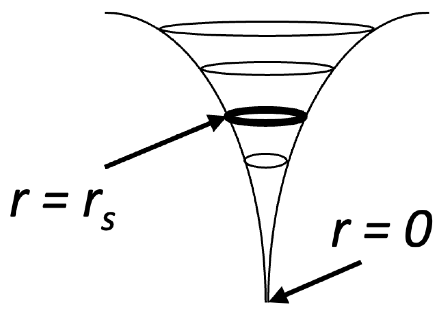
Figure 3.
Surface of Constant for the Exterior Metric in Kruskal-Szekeres Coordinates.
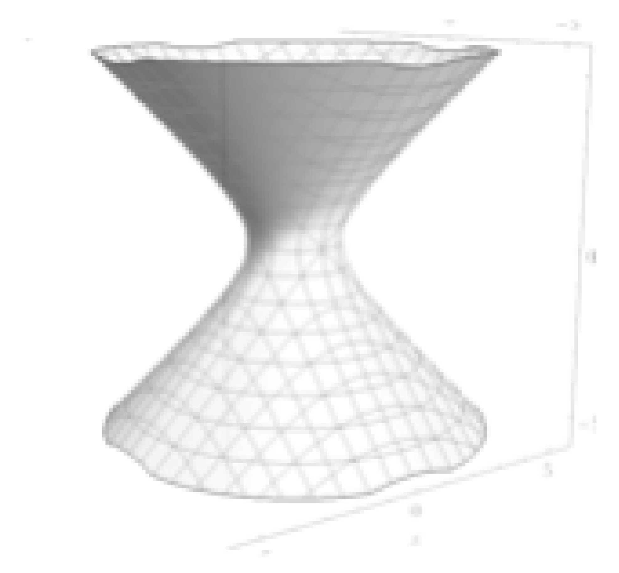
Figure 4.
Surface of Constant for the Interior Metric in Kruskal-Szekeres Coordinates.
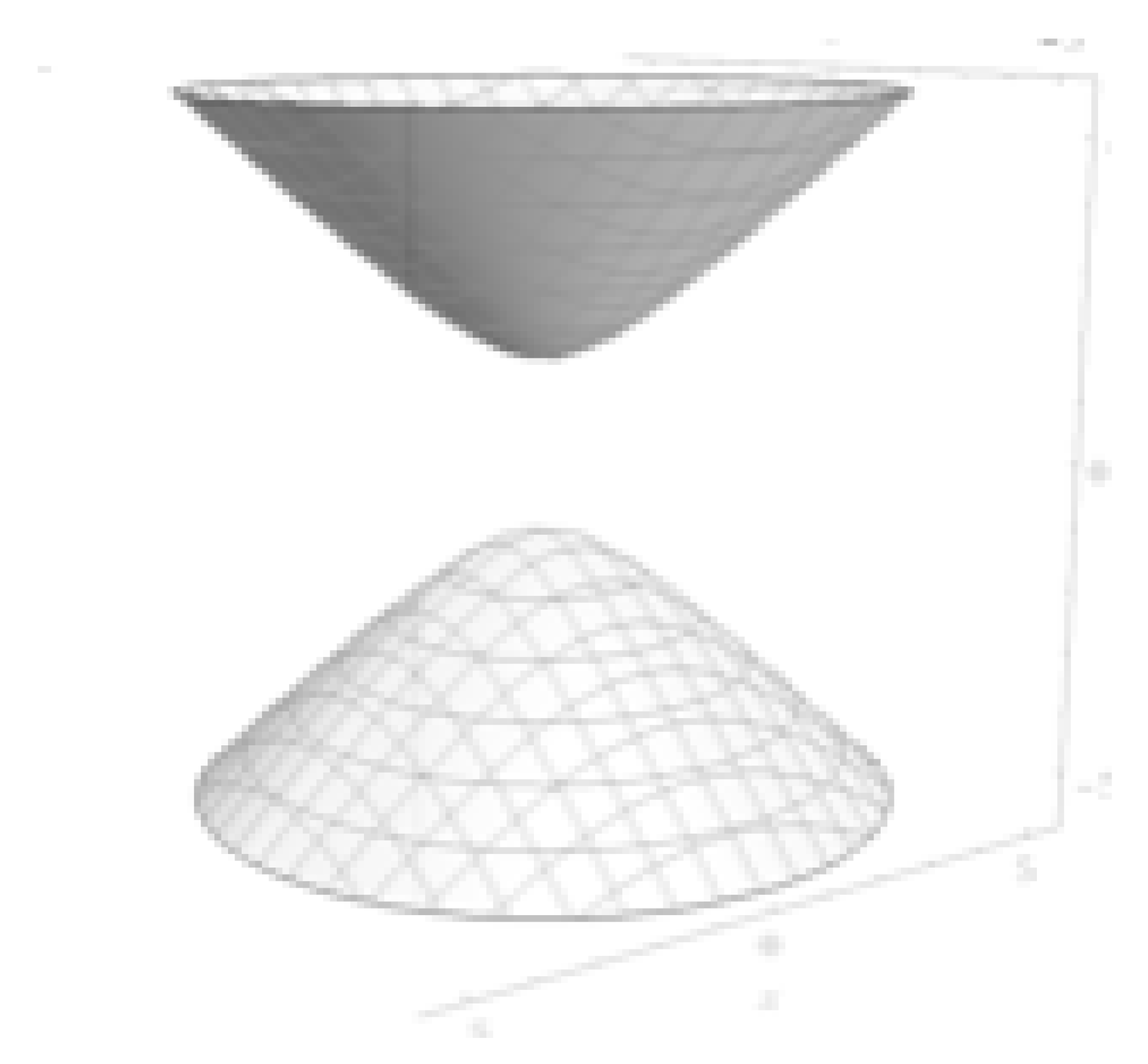
Figure 5.
Parallel Transport of Normal Vectors on a Spherical Surface.
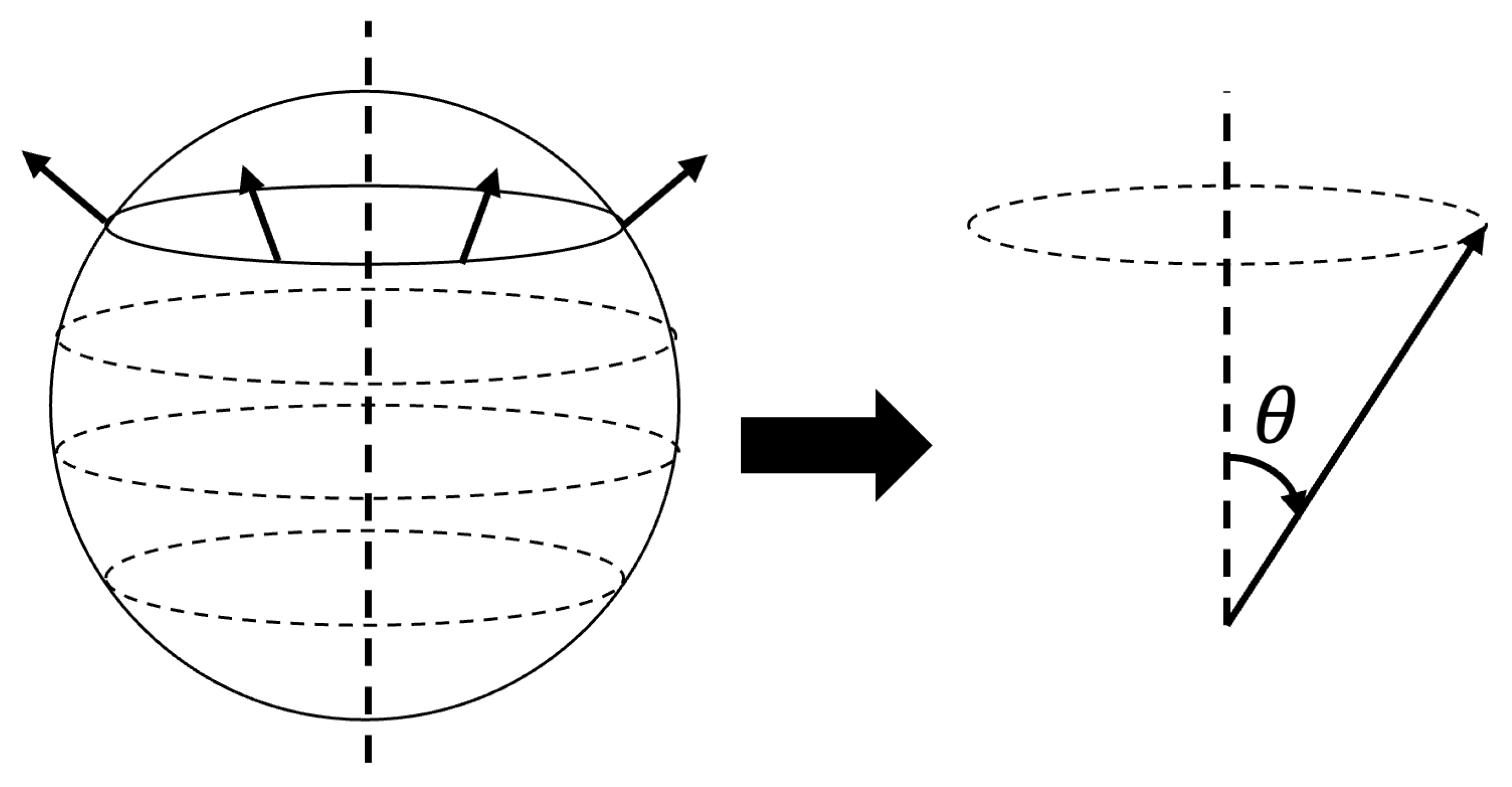
Figure 6.
Parallel Transport of Normal Vectors on a Hyperbolic Surface.
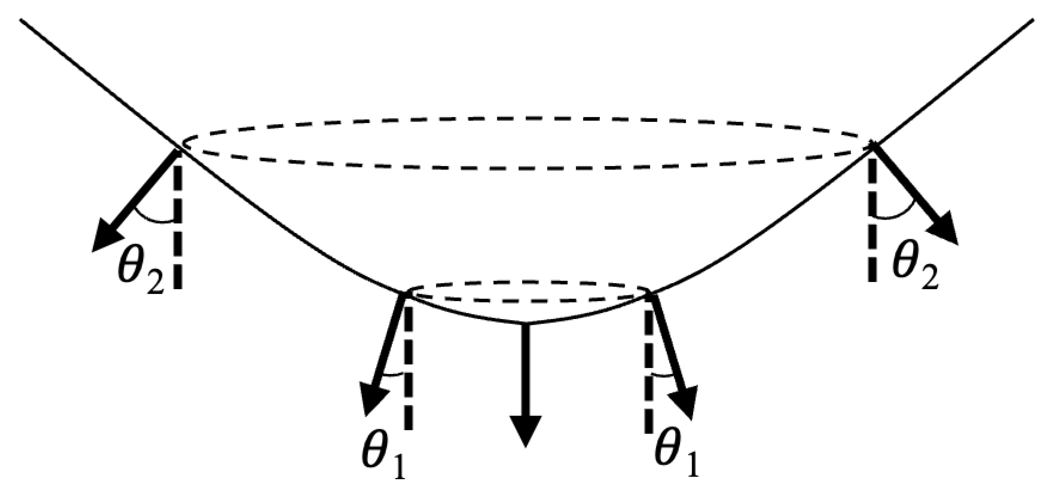
Figure 7.
Velocity Vector of an Orbiting Observer in Kruskal-Szekeres Coordinate.
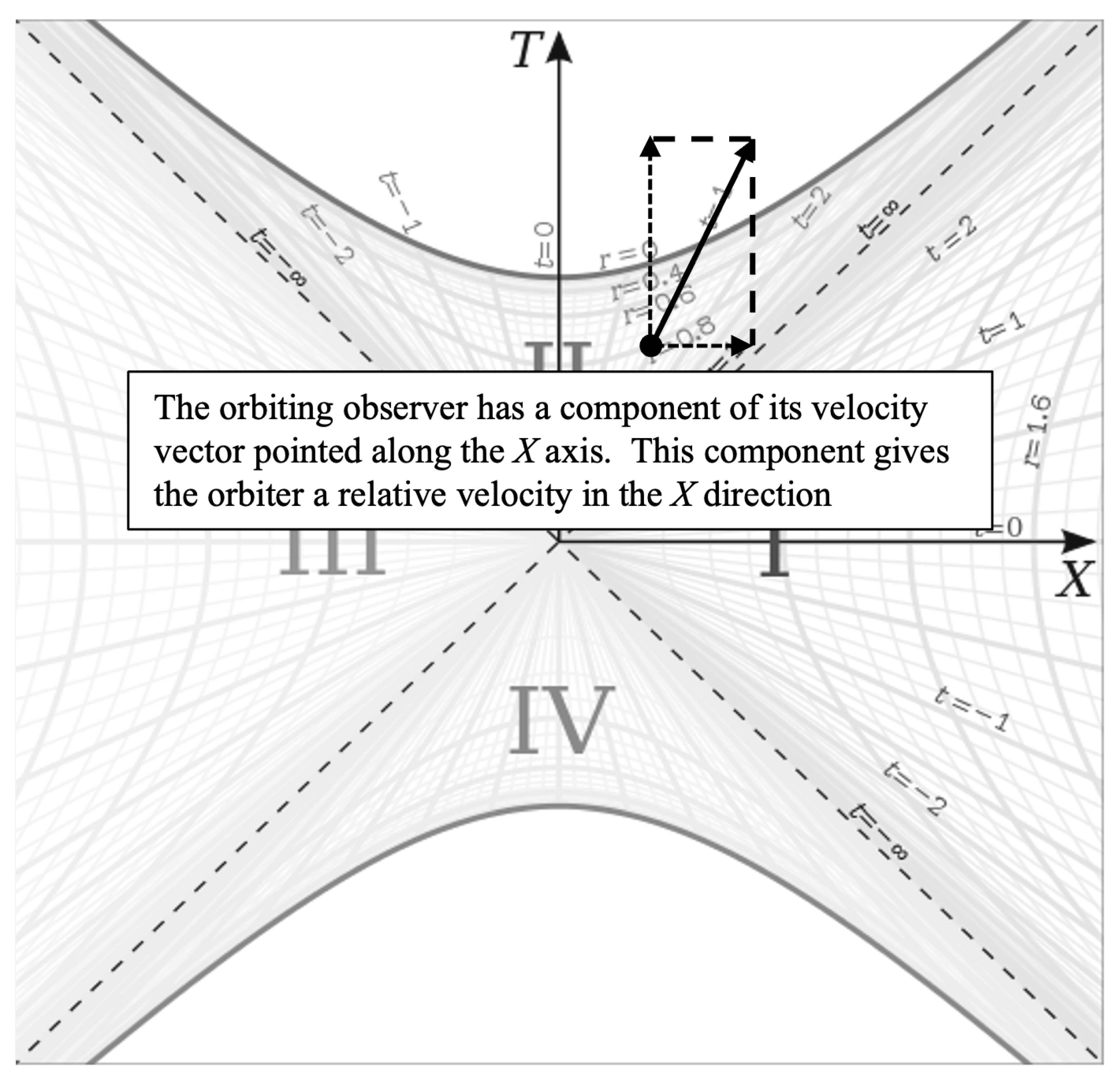
Figure 8.
Velocity Vector of an Orbiting Observer in Kruskal-Szekeres Coordinate.
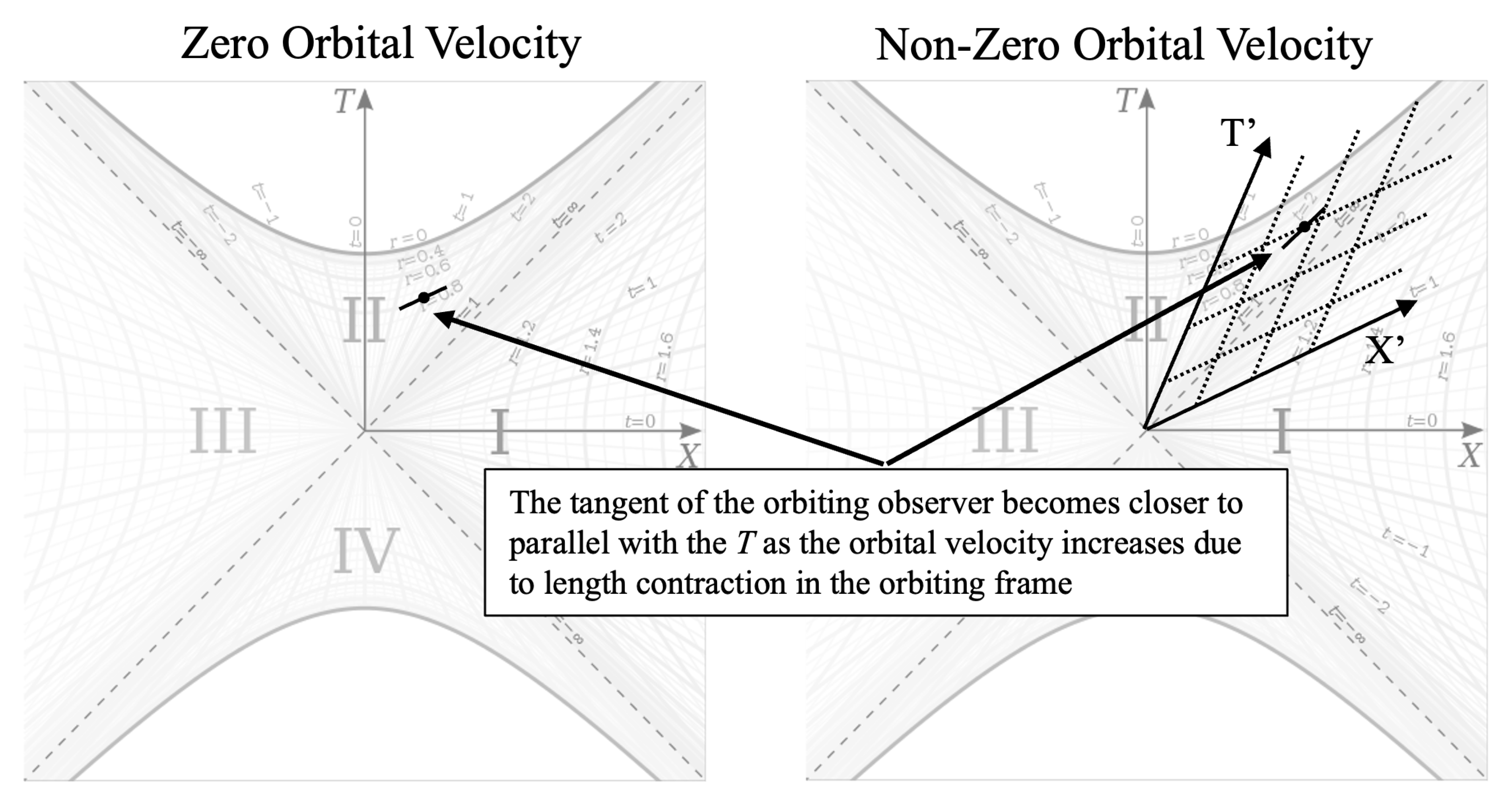
Figure 9.
Deformation of Surface of Constant Time by a Black Hole in Minkowski Space.
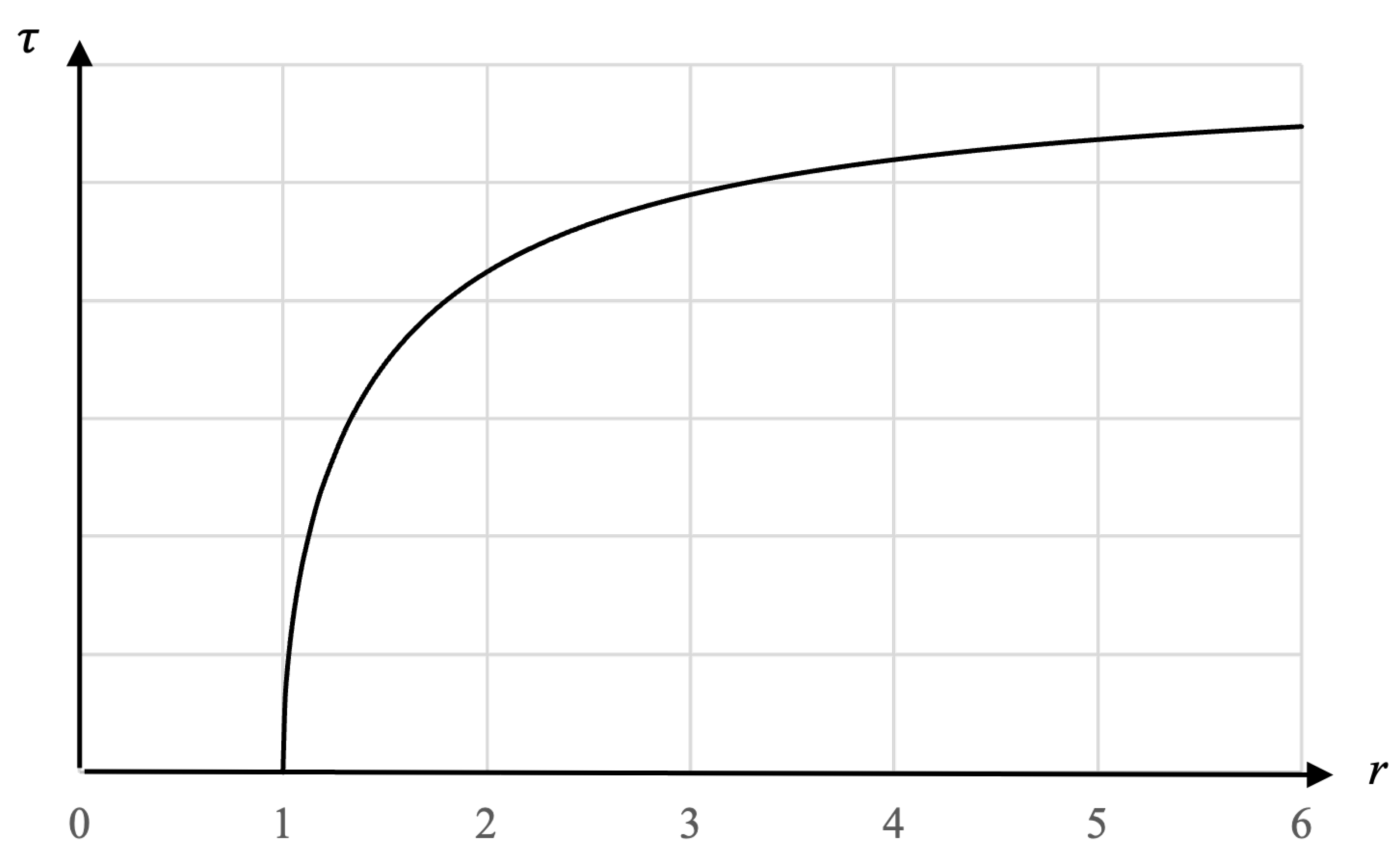
Figure 10.
Deforming a Surface of Constant Time by a Black Hole in the Interior Schwarzschild Metric.
Figure 10.
Deforming a Surface of Constant Time by a Black Hole in the Interior Schwarzschild Metric.
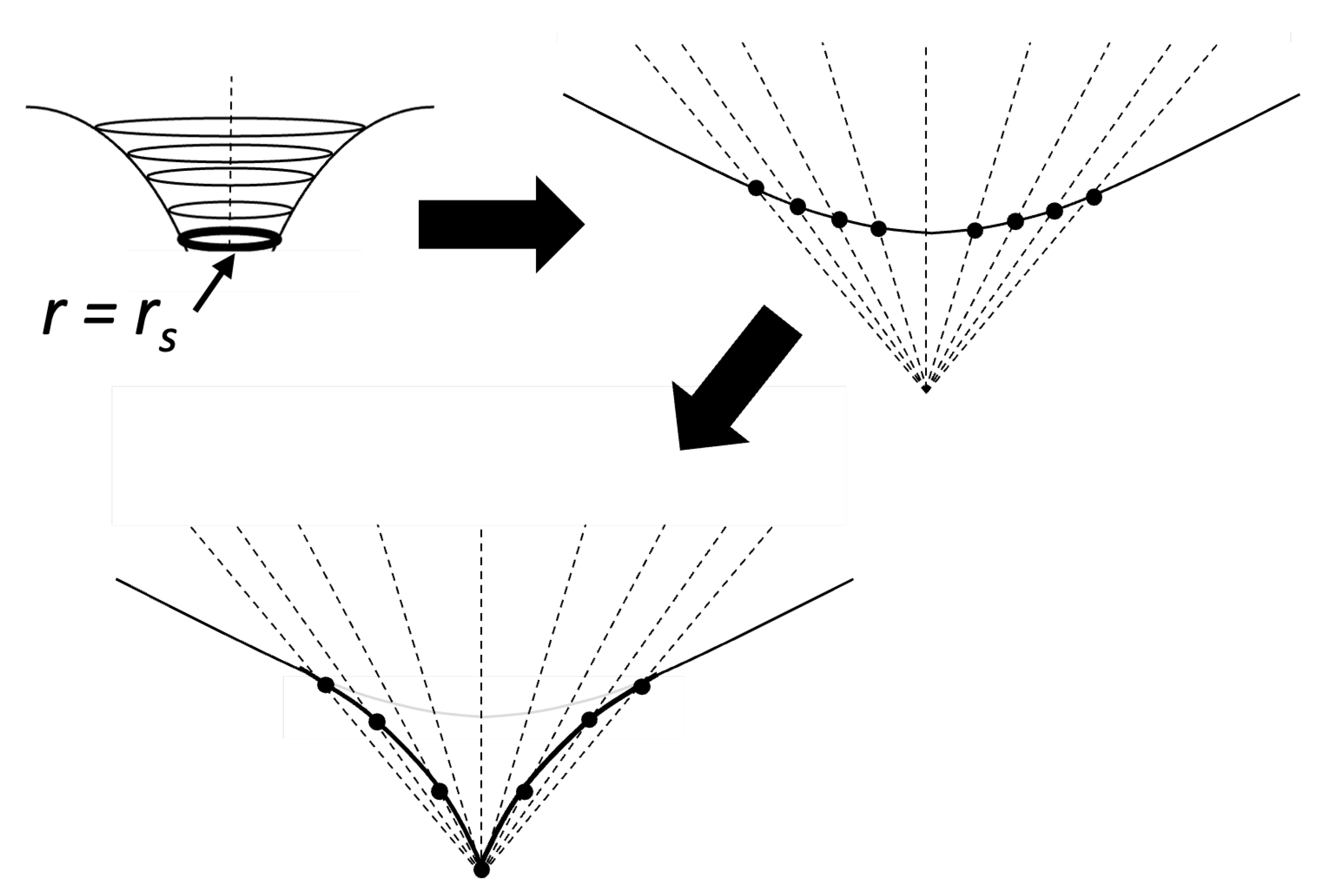
Figure 11.
Deformation of Surface of Constant Time by a Black Hole in the Interior Schwarzschild Metric.
Figure 11.
Deformation of Surface of Constant Time by a Black Hole in the Interior Schwarzschild Metric.
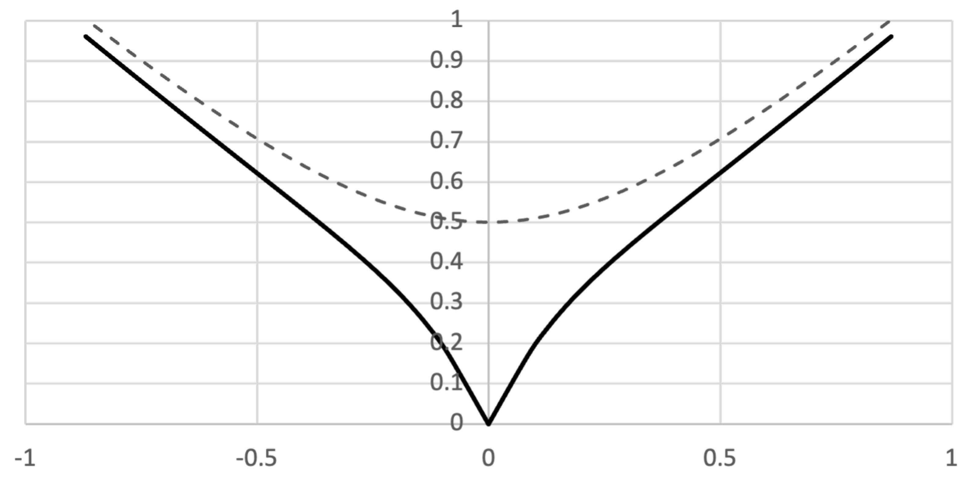
Figure 12.
Scale Factor vs. r for .
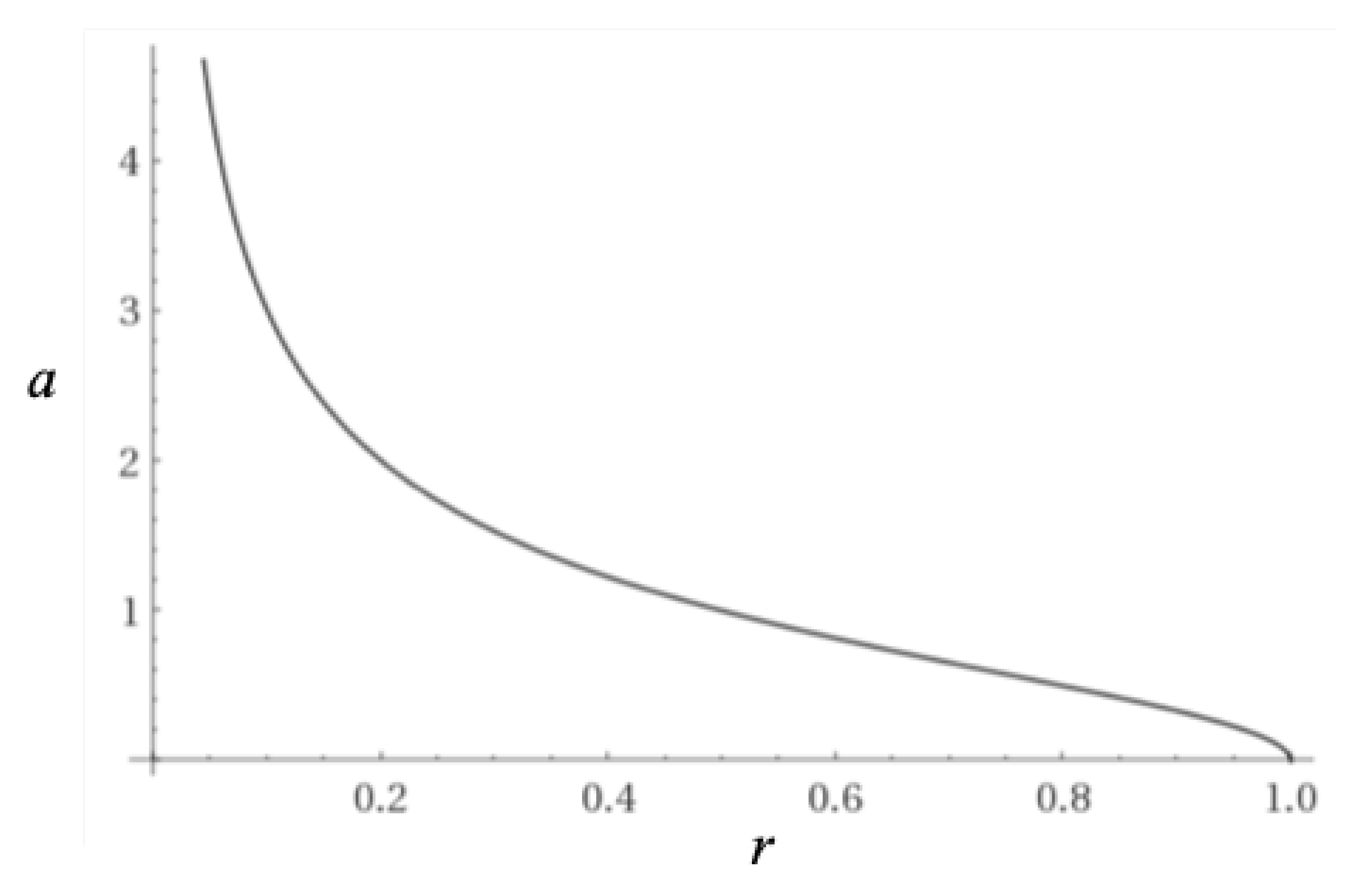
Figure 13.
Distance Modulus vs. Redshift Plotted with Supernova Measurements.
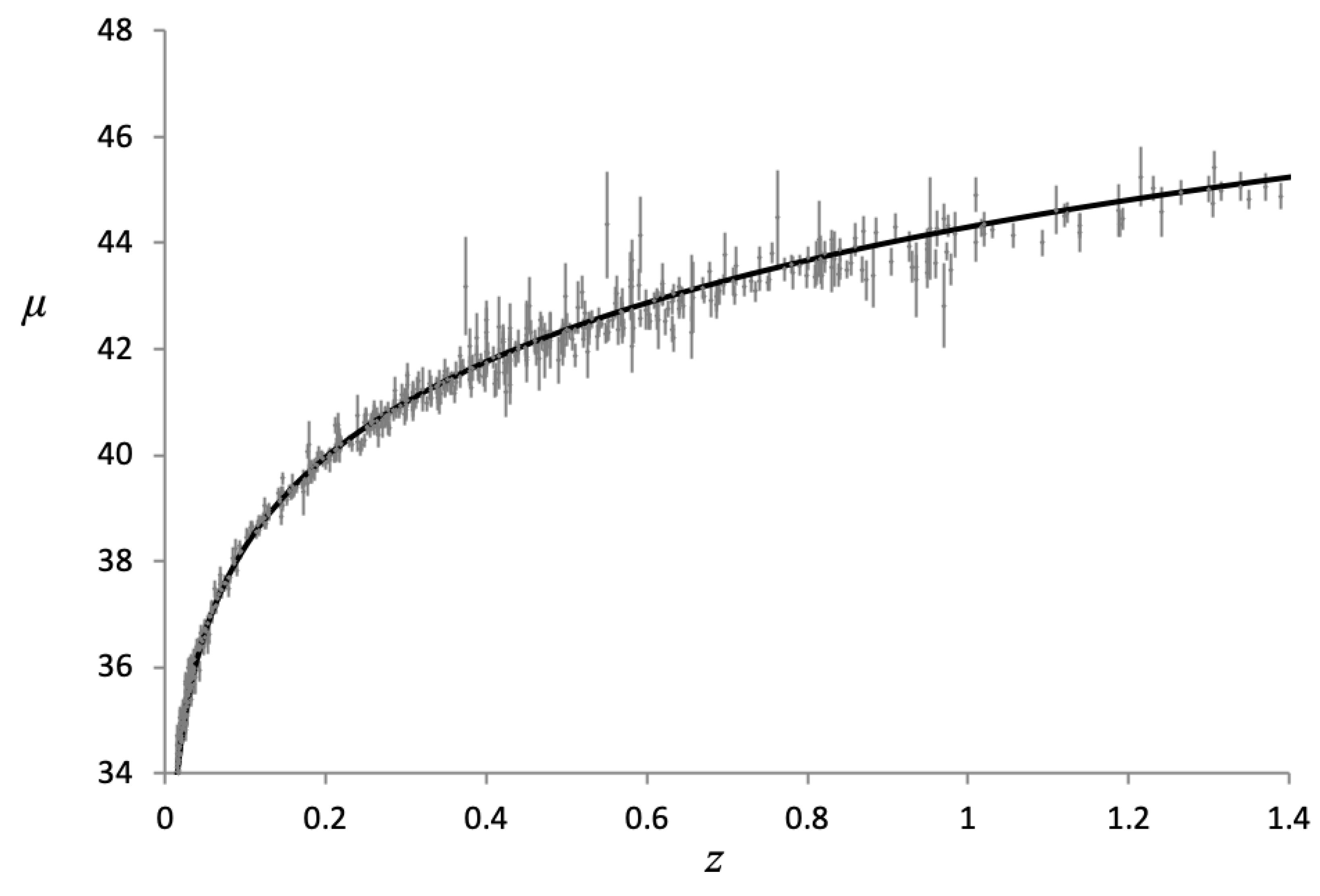
Figure 14.
Distance Modulus vs. Redshift Plotted with Quasar Measurements.
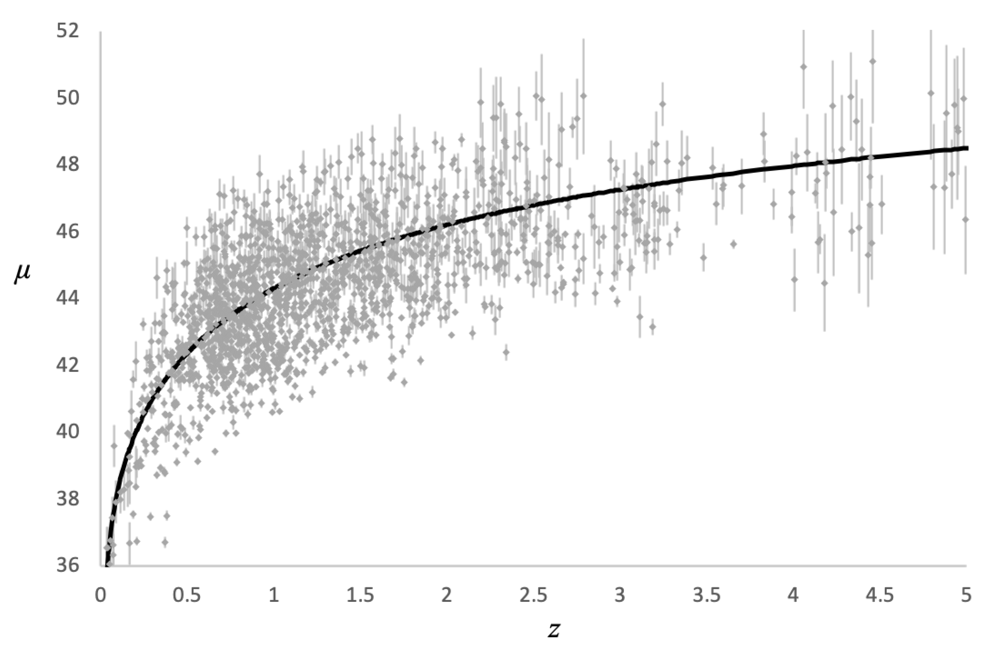
Figure 15.
Distance Modulus vs. Redshift Comparison with CDM.
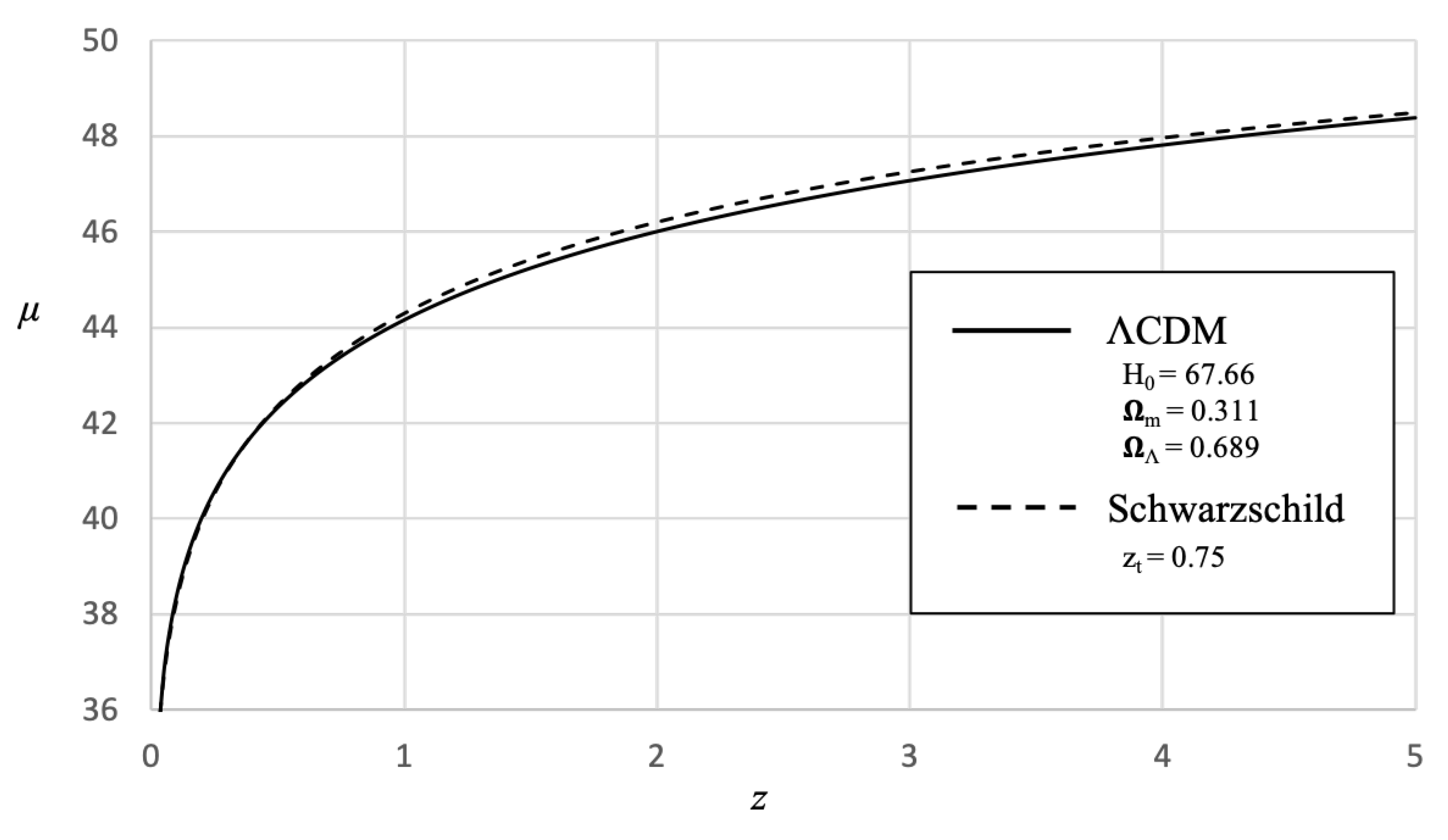
Figure 16.
Lookback Time vs. Redshift.
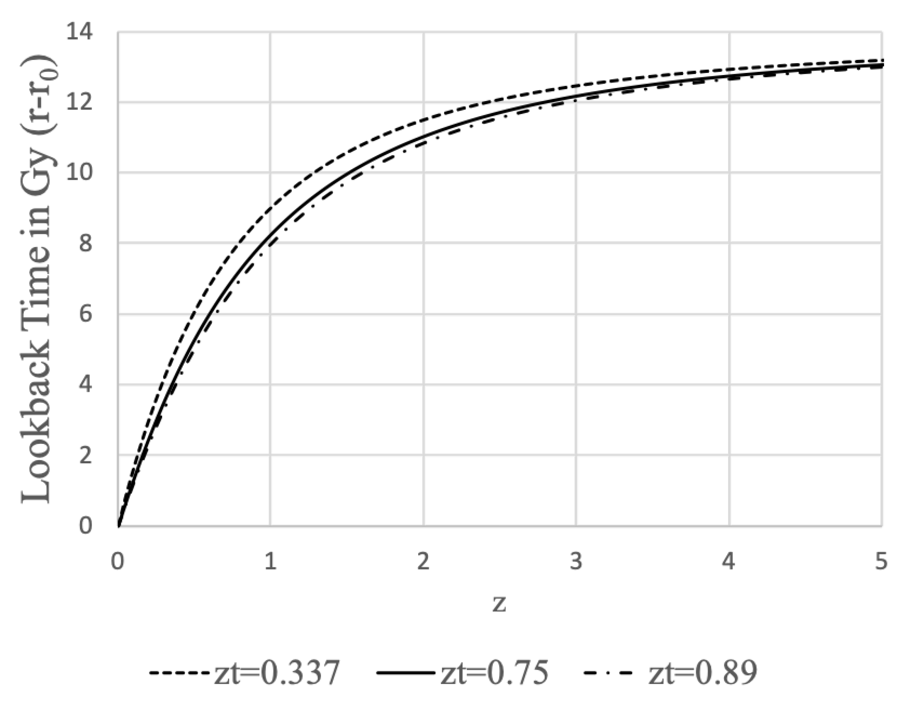
Figure 17.
Universe and Antiverse.
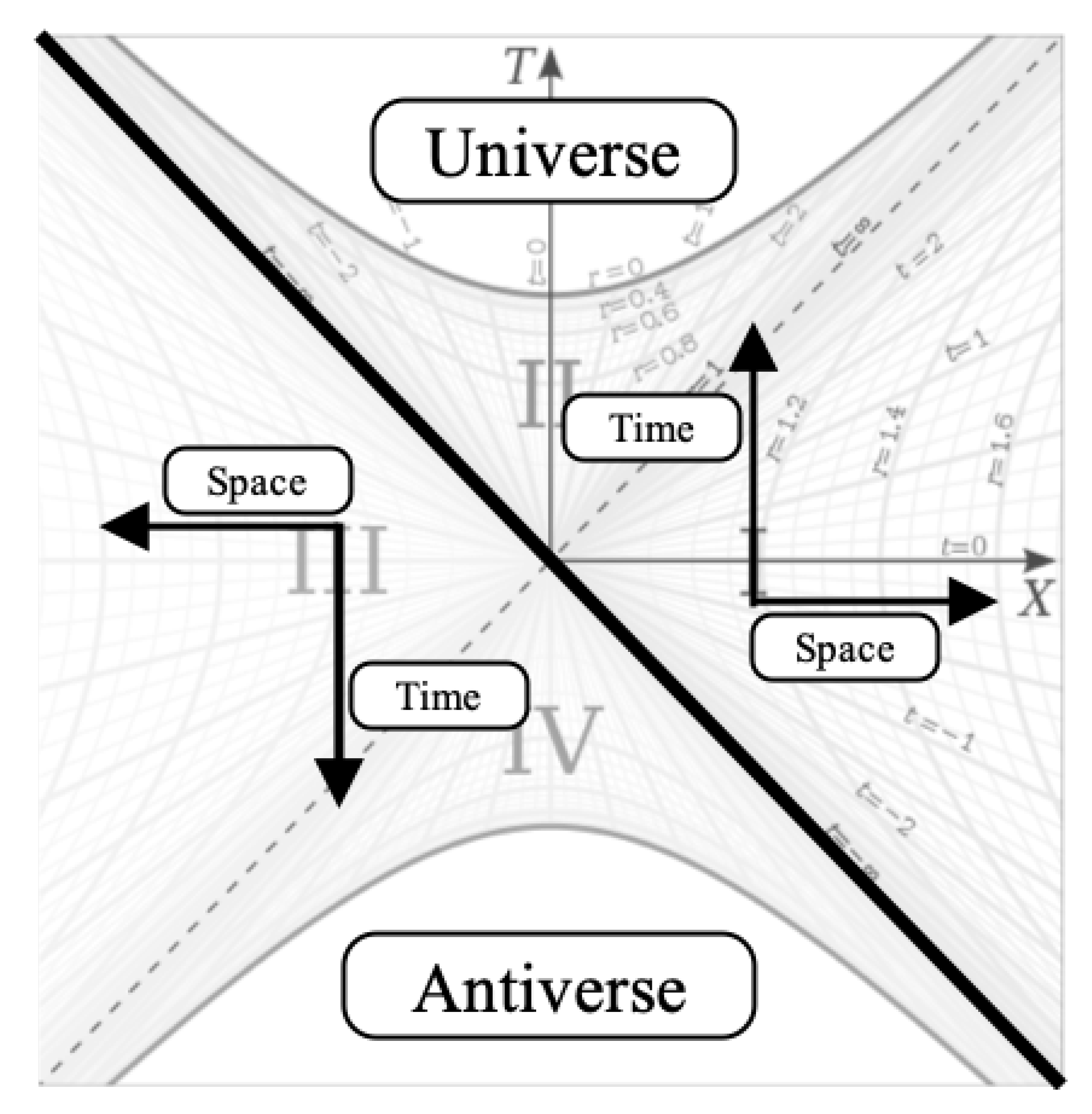

Table 1.
Limiting Cosmological Parameter Values Based on Measurement and a 13.8 Gy Age of the Universe.
Table 1.
Limiting Cosmological Parameter Values Based on Measurement and a 13.8 Gy Age of the Universe.
| u | ||||||||
| 0.337 | 13.8 | 37.0 | 23.2 | 56.6 | 0.77 | -0.49 | 0.0007 | 0.99 |
| 0.75 | 13.8 | 27.3 | 13.5 | 71.6 | 1.01 | -1.02 | 0.0009 | 0.99 |
| 0.89 | 13.8 | 25.4 | 11.6 | 77.6 | 1.09 | -1.17 | 0.0010 | 0.99 |
Table 2.
Limiting Proper Times Based on Measurements and an age of 13.8 Gy for the Universe (Time is in Gy).
Table 2.
Limiting Proper Times Based on Measurements and an age of 13.8 Gy for the Universe (Time is in Gy).
| 0.337 | 13.8 | 42.2 | 58.1 | 15.9 |
| 0.75 | 13.8 | 35.2 | 42.9 | 7.7 |
| 0.89 | 13.8 | 33.7 | 39.9 | 6.2 |
Disclaimer/Publisher’s Note: The statements, opinions and data contained in all publications are solely those of the individual author(s) and contributor(s) and not of MDPI and/or the editor(s). MDPI and/or the editor(s) disclaim responsibility for any injury to people or property resulting from any ideas, methods, instructions or products referred to in the content. |
© 2024 by the authors. Licensee MDPI, Basel, Switzerland. This article is an open access article distributed under the terms and conditions of the Creative Commons Attribution (CC BY) license (http://creativecommons.org/licenses/by/4.0/).
Copyright: This open access article is published under a Creative Commons CC BY 4.0 license, which permit the free download, distribution, and reuse, provided that the author and preprint are cited in any reuse.


