Preprint
Article

This version is not peer-reviewed.

A Proof of the Riemann Hypothesis Based on a New Expression of the Completed Zeta Function

Submitted:

07 January 2025

Posted:

07 January 2025

Read the latest preprint version here

Abstract

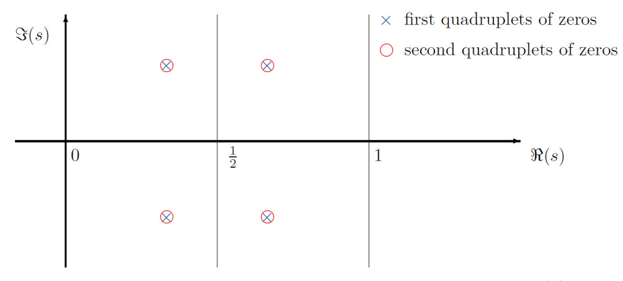
The Riemann Hypothesis (RH) is proved based on a new expression of the completed zeta function $\xi(s)$, which was obtained through paring the conjugate zeros $\rho_i$ and $\bar{\rho}_i$ in the Hadamard product, with consideration of the multiplicity of zeros, i.e. $$\xi(s)=\xi(0)\prod_{\rho}(1-\frac{s}{\rho})=\xi(0)\prod_{i=1}^{\infty}(1-\frac{s}{\rho_i})(1-\frac{s}{\bar{\rho}_i})=\xi(0)\prod_{i=1}^{\infty}\Big{(}\frac{\beta_i^2}{\alpha_i^2+\beta_i^2}+\frac{(s-\alpha_i)^2}{\alpha_i^2+\beta_i^2}\Big{)}^{m_{i}}$$ where $\xi(0)=\frac{1}{2}$, $\rho_i=\alpha_i+j\beta_i$ and $\bar{\rho}_i=\alpha_i-j\beta_i$ are the complex conjugate zeros of $\xi(s)$, $0<\alpha_i<1$ and $\beta_i\neq 0$ are real numbers, $m_i\geq 1$ is the multiplicity of $\rho_i$, finite and unique, $0<|\beta_1|\leq|\beta_2|\leq \cdots$. Then, according to the functional equation $\xi(s)=\xi(1-s)$, we have $$\prod_{i=1}^{\infty}\Big{(}1+\frac{(s-\alpha_i)^2}{\beta_i^2}\Big{)}^{m_{i}}=\prod_{i=1}^{\infty}\Big{(}1+\frac{(1-s-\alpha_i)^2}{\beta_i^2}\Big{)}^{m_{i}}$$ Owing to the divisibility contained in the above equation and the uniqueness of $m_i$, it is equivalent to $$\Big{(}1+\frac{(s-\alpha_i)^2}{\beta_i^2}\Big{)}^{m_{i}}=\Big{(}1+\frac{(1-s-\alpha_i)^2}{\beta_i^2}\Big{)}^{m_{i}}, i=1, 2, 3, \dots, \infty $$ which is further equivalent to $$\alpha_i=\frac{1}{2}, 0<|\beta_1|<|\beta_2|<|\beta_3|<\cdots, i=1, 2, 3, \dots, \infty$$

Thus we conclude that the RH is true.

Keywords: 
;  ;  

1. Introduction

The RH [1] is one of the most important unsolved problems in mathematics. Although there are many achievements towards proving this celebrated hypothesis, it remains an open problem [2,3]. The Riemann zeta function is originally defined in the half-plane ( s ) > 1 by the absolutely convergent series [2]
ζ ( s ) = n = 1 1 n s , ( s ) > 1
The connection between the above-defined Riemann zeta function and prime numbers was discovered by Euler, i.e., the famous Euler product
ζ ( s ) = n = 1 1 n s = p ( 1 p s ) 1 , ( s ) > 1
where p runs over the prime numbers.
Riemann showed in his paper in 1859 how to extend the zeta function to the whole complex plane C by analytic continuation, i.e.
ζ ( s ) = Γ ( 1 s ) 2 π i ( x ) s e x 1 · d x x
where " " is the symbol adopted by Riemann to represent the contour integral from + to + around a domain which includes the value 0 but no other point of discontinuity of the integrand in its interior.
Or equivalently,
ζ ( s ) = π s / 2 Γ ( s / 2 ) { 1 s ( s 1 ) + 1 ( x s 2 1 + x s 2 1 2 ) · ( θ ( x ) 1 2 ) d x }
where θ ( x ) = e n 2 π x is the Jaccobi theta function, Γ is the Gamma function in the following Weierstrass expression
1 Γ ( s ) = s · e γ s n = 1 ( 1 + s n ) e s / n
where γ is the Euler-Mascheroni constant.
As shown by Riemann, ζ ( s ) extends to C as a meromorphic function with only a simple pole at s = 1 , with residue 1, and satisfies the following functional equation
π s 2 Γ ( s 2 ) ζ ( s ) = π 1 s 2 Γ ( 1 s 2 ) ζ ( 1 s )
The Riemann zeta function ζ ( s ) has zeros at the negative even integers: 2 , 4 , 6 , 8 , ⋯ and one refers to them as the trivial zeros. The other zeros of ζ ( s ) are the complex numbers, i.e., non-trivial zeros [2].
In 1896, Hadamard [4] and Poussin [5] independently proved that no zeros could lie on the line ( s ) = 1 , together with the functional equation ξ ( s ) = ξ ( 1 s ) and the fact that there are no zeros with real part greater than 1, this showed that all non-trivial zeros must lie in the interior of the critical strip 0 < ( s ) < 1 . Later on, Hardy (1914) [6], Hardy and Littlewood (1921) [2] showed that there are infinitely many zeros on the critical line ( s ) = 1 2 .
To give a summary of the related research works on the RH, we have the following results on the properties of the non-trivial zeros of ζ ( s ) [4,5,6,7,8,9].
Lemma 1: Non-trivial zeroes of ζ ( s ) , noted as ρ = α + j β , have the following properties
1) The number of non-trivial zeroes is infinity;
2) β 0 ;
3) 0 < α < 1 ;
4) ρ , ρ ¯ , 1 ρ ¯ , 1 ρ are all non-trivial zeroes.
As further study, a completed zeta function ξ ( s ) is proposed by equation
ξ ( s ) = 1 2 s ( s 1 ) π s 2 Γ ( s 2 ) ζ ( s )
It is well-known that ξ ( s ) is an entire function of order 1. This implies ξ ( s ) is analytic, and can be expressed as infinite product of polynomial factors, in the whole complex plane C . In addition, replacing s with 1 s in Eq.(6), and combining Eq.(5), we obtain the following functional equation
ξ ( s ) = ξ ( 1 s )
According to the definition of ξ ( s ) , and recalling Eq.(4), the trivial zeros of ζ ( s ) are canceled by the poles of Γ ( s 2 ) . The zero of s 1 and the pole of ζ ( s ) cancel; the zero s = 0 and the pole of Γ ( s 2 ) cancel [9,10]. Thus, all the zeros of ξ ( s ) are exactly the nontrivial zeros of ζ ( s ) . Then we have the following Lemma 2.
Lemma 2: The zeros of ξ ( s ) coincide with the non-trivial zeros of ζ ( s ) .
Consequently, the following two statements are equivalent.
Statement 1: All the non-trivial zeros of ζ ( s ) have real part equal to 1 2 .
Statement 2: All zeros of ξ ( s ) have real part equal to 1 2 .
To prove the RH, a natural thinking is to estimate the numbers of non-trivial zeros of ζ ( s ) inside or outside some certain areas according to Argument Principle. Along this train of thought, there are many research works. Let N ( T ) denote the number of non-trivial zeros of ζ ( s ) inside the rectangle: 0 < α < 1 , 0 < β T , and let N 0 ( T ) denote the number of non-trivial zeros of ζ ( s ) on the line α = 1 2 , 0 < β T . Selberg proved that there exist positive constants c and T 0 , such that N 0 ( T ) > c N ( T ) , ( T > T 0 ) [11], later on, Levinson proved that c 1 3 [12], Lou and Yao proved that c 0.3484 [13], Conrey proved that c 2 5 [14], Bui, Conrey and Young proved that c 0.41 [15], Feng proved that c 0.4128 [16], Wu proved that c 0.4172 [17].
On the other hand, many non-trivial zeros have been calculated by hand or by computer programs. Among others, Riemann found the first three non-trivial zeros [18]. Gram found the first 15 zeros based on Euler-Maclaurin summation [19]. Titchmarsh calculated the 138th to 195th zeros using the Riemann-Siegel formula [20,21]. Here are the first three (pairs of) non-trivial zeros: 1 2 ± j 14.1347251 ; 1 2 ± j 21.0220396 ; 1 2 ± j 25.0108575 .
The idea of this paper is originated from Euler’s work on proving the following famous equality
1 + 1 2 2 + 1 3 2 + 1 4 2 + 1 5 2 + = π 2 6
This interesting result is deduced by comparing the like terms of two types of infinite expressions, i.e., infinite polynomial and infinite product, as shown in the following
sin x x = 1 x 2 3 ! + x 4 5 ! x 6 7 ! + = ( 1 x 2 π 2 ) ( 1 x 2 4 π 2 ) ( 1 x 2 9 π 2 )
Then the author of this paper conjectured that ξ ( s ) should be factored into ( 1 + ( s α i ) 2 β i 2 ) or something like that, which was verified by paring ρ i and ρ ¯ i in the Hadamard product of ξ ( s ) , i.e. ( 1 s ρ i ) ( 1 s ρ ¯ i ) = β i 2 α i 2 + β i 2 ( 1 + ( s α i ) 2 β i 2 )
The Hadamard product of ξ ( s ) as shown in Eq.(10) was first proposed by Riemann, however, it was Hadamard who showed the validity of this infinite product expansion [22].
ξ ( s ) = ξ ( 0 ) ρ ( 1 s ρ )
where ξ ( 0 ) = 1 2 , ρ runs over all zeros of ξ ( s ) .
Hadamard pointed out that to ensure the absolute convergence of the infinite product expansion, ρ and 1 ρ are paired. Later in Section 4, we will show that ρ and ρ ¯ can also be paired to ensure the absolute convergence of the infinite product expansion.

2. Preliminary Lemmas

This section provides some preliminary knowledge to support the proof of the key lemma - Lemma 10 in next section. We need the classical results (Lemma 3 and Lemma 4) in polynomial algebra over fields, with extension to infinite product of polynomial factors (Lemma 5, Lemma 6, and Lemma 7), and properties of the multiplicity of zeros of the entire function (Lemma 8 and Lemma 9).
In the remainder of this paper, we focus on polynomials with real coefficients and infinite products of polynomial factors with real coefficients (absolutely convergent on the whole complex plane), both of which are types of entire functions.
To begin with, we introduce the ring of polynomial, denoted as R [ x ] , which is defined as the set of all polynomials in x over the field of real numbers R , i.e.
R [ x ] = { i = 0 a i x i | a i R , a i 0 for all but a finite number of i }
The set R [ x ] equipped with the operations + (addition) and · (multiplication) is the ring of polynomial in x over the field R .
According to Reference [27], the ring of polynomial is a subset of the ring of entire function, and both rings possess divisibility property.
Definition: Let f ( x ) = i = 1 p i ( x ) , p i ( x ) R [ x ] , be an infinite product of polynomial factors, and let h ( x ) R [ x ] . If there exists an infinite product of polynomial factors g ( x ) = i = 1 q i ( x ) , q i ( x ) R [ x ] , such that: f ( x ) = h ( x ) · g ( x ) , then h ( x ) is said to divide f ( x ) , denoted as h ( x ) f ( x ) .
Remark: The above definition implicitly assumes the absolute convergence of the infinite product of polynomial factors, because f ( x ) = h ( x ) · g ( x ) is obtained through rearrangement of factors of f ( x ) .
Lemma 3: Let m ( x ) , g 1 ( x ) , . . . , g n ( x ) R [ x ] , n 2 . If m ( x ) is irreducible (prime) and divides the product g 1 ( x ) g n ( x ) , then m ( x ) divides one of the polynomials g 1 ( x ) , . . . , g n ( x ) .
Lemma 4: Let f ( x ) , m ( x ) R [ x ] . If m ( x ) is irreducible and f ( x ) is any polynomial, then either m ( x ) divides f ( x ) or g c d ( m ( x ) , f ( x ) ) = 1 , (gcd: greatest common divisor).
Lemma 5: Let m ( x ) , g 1 ( x ) , g 2 ( x ) , R [ x ] . If m ( x ) is irreducible and divides the infinite product i = 1 g i ( x ) , then m ( x ) divides one of the polynomials g 1 ( x ) , g 2 ( x ) , .
Lemma 6: Let q ( x ) , m ( x ) , p 1 ( x ) , p 2 ( x ) , R [ x ] , p ( x ) = i = 1 p i ( x ) . If m ( x ) is irreducible and divides the product q ( x ) p ( x ) , but m ( x ) and p ( x ) are relative prime, then m ( x ) divides q ( x ) .
Lemma 7: Let m ( x ) , p 1 ( x ) , p 2 ( x ) , R [ x ] , p ( x ) = i = 1 p i ( x ) . If m ( x ) is irreducible, then either m ( x ) divides p ( x ) , or m ( x ) and p ( x ) are relative prime, i.e., g c d ( m ( x ) , p ( x ) ) = 1 .
Remark: The contents of Lemma 3 and Lemma 4 can be found in many textbooks of linear algebra, modern algebra, or abstract algebra, see for example references [24,25,26]. Below we give the proofs of Lemma 5, Lemma 6, and Lemma 7.
Proof of Lemma 5: The proof is conducted by Transfinite Induction.
Let P ( γ ) ( γ is an ordinal number) be the statement:
" m ( x ) , g 1 ( x ) , . . . , g γ ( x ) R [ x ] , γ 2 . If m ( x ) is irreducible and divides the product g 1 ( x ) g γ ( x ) , then m ( x ) divides one of the polynomials g 1 ( x ) , . . . , g γ ( x ) ", where γ A , A = N { ω } with the ordering that n < ω for all natural numbers n, ω is the smallest limit ordinal other than 0.
Base Case: P ( 2 ) is an obvious fact according to Lemma 3 with n = 2 ;
Successor Case: To prove P ( γ ) P ( γ + 1 ) , we have g 1 ( x ) g γ ( x ) g γ + 1 ( x ) = g ( x ) · g γ + 1 ( x ) , where g ( x ) = g 1 ( x ) g γ ( x ) . Then according to Lemma 3 with n = 2 , we have m ( x ) g ( x ) · g γ + 1 ( x ) m ( x ) g ( x ) or m ( x ) g γ + 1 ( x ) . Considering P ( γ ) : if m ( x ) divides g ( x ) , then m ( x ) divides one of g 1 ( x ) , , g γ ( x ) , thus we know P ( γ ) P ( γ + 1 ) .
Limit Case: We need to prove P ( γ < λ ) P ( λ ) , λ is any limit ordinal other than 0. For the sake of contradiction, assume that P ( γ < λ ) P ( λ ) , i.e., m ( x ) does not divide any polynomial g i ( x ) , 1 i λ . Then, considering m ( x ) is irreducible with the property stated in Lemma 4, we have:
m ( x ) | g 1 ( x ) g γ ( x ) ( by transitivity of divisibility ) m ( x ) | g 1 ( x ) g γ g λ ( x ) ( by the assumption and Lemma 4 ) g c d ( m ( x ) , g i ( x ) ) = 1 , 1 i λ ( for all natural numbers n N , n < λ ) g c d ( m ( x ) , g i ( x ) ) = 1 , i N
which contradicts P ( γ < λ ) : m ( x ) | g 1 ( x ) g γ ( x ) m ( x ) divides one of the polynomials g 1 ( x ) , . . . , g γ ( x ) , γ N . Thus, we know that the assumption P ( γ < λ ) P ( λ ) is false.
Then P ( γ < λ ) P ( λ ) is true, i.e., the Limit Case is true.
That completes the proof of Lemma 5.
Proof of Lemma 6: If m ( x ) is irreducible and divides the product q ( x ) p ( x ) , then according to Lemma 5, m ( x ) divides one of the polynomials q ( x ) , p 1 ( x ) , p 2 ( x ) , . . . . Further, if m ( x ) and p ( x ) are relative prime, then m ( x ) does not divides any factor p i ( x ) , i = 1 , , of p ( x ) (otherwise m ( x ) divides p ( x ) , which contradicts the condition " m ( x ) and p ( x ) are relative prime"). Thus, m ( x ) must divides q ( x ) .
That completes the proof of Lemma 6.
Proof of Lemma 7:
Since m ( x ) is irreducible, then by the definition of irreducible polynomial, either g c d ( m ( x ) , p ( x ) ) = k · m ( x ) , k R , k 0 or g c d ( m ( x ) , p ( x ) ) = 1 . It is clear that g c d ( m ( x ) , p ( x ) ) = k · m ( x ) m ( x ) p ( x ) . Thus, we conclude that either m ( x ) divides p ( x ) or g c d ( m ( x ) , p ( x ) ) = 1 , i.e., m ( x ) and p ( x ) are relative prime.
That completes the proof of Lemma 7.
Additionally, we also need the following results on properties of a zero of entire function in complex analysis for understanding the multiplicity of a zero of ξ ( s ) .
Lemma 8: Let f ( s ) be a non-zero entire function, and let s 0 be a zero of f ( s ) . Then the multiplicity of s 0 is a finite positive integer.
Proof: Let f ( s ) ¬ 0 , s C , be an entire function, which means it is holomorphic on the whole complex plane. Suppose f ( s ) has a zero at s 0 C of multiplicity m, then f ( s ) = ( s s 0 ) m g ( s ) , where g ( s ) is also an entire function and g ( s 0 ) 0 .
Assume for contradiction that m is infinite, which implies there exists an accumulation point of zeros in the neighbor of s 0 . Then, by Identity Theorem for holomorphic functions, and considering "0" is also an entire function, we have f ( s ) 0 , s C , which contradicts the given condition that f ( s ) ¬ 0 , s C . Thus, the assumption is false, i.e., m must be a finite positive integer.
That completes the proof of Lemma 8.
Remark: Statements similar to Lemma 8 can be found in Reference [28] and other related textbooks/monographs.
Lemma 9: Let f ( s ) be a non-zero entire function, and let s 0 be a zero of f ( s ) . Then the multiplicity of s 0 is unique.
Proof: Let f ( s ) ¬ 0 , s C , be an entire function, which has a multiple zero at s 0 C of multiplicity m. We can write: f ( s ) = ( s s 0 ) m g ( s ) , where g ( s ) is also an entire function and g ( s 0 ) 0 .
Assume for contradiction that there exists another integer n m such that n is also a multiplicity of the zero s 0 . This means we can also write: f ( s ) = ( s s 0 ) n h ( s ) , where h ( s ) is an entire function and h ( s 0 ) 0 .
Since both expressions for f ( s ) must be equal, we then obtain ( s s 0 ) m g ( s ) = ( s s 0 ) n h ( s ) . Without loss of generality, consider m > n , then we have: ( s s 0 ) m n g ( s ) = h ( s ) h ( s 0 ) = 0 , which is a contradiction to h ( s 0 ) 0 . Thus, the assumption is false, i.e., the multiplicity of a zero of any non-zero entire function is unique.
That completes the proof of Lemma 9.

3. Key Lemma

In this section, we first explain the multiplicity of a quadruplets of zeros of ξ ( s ) / ξ ( 1 s ) , which is used to facilitate the identification of unreasonable subsequent multiple zeros. After that we prove the key lemma - Lemma 10, which is substantial for the proof of the RH.
Multiple zeros of ξ ( s ) / ξ ( 1 s ) : As shown in Figure 1, the multiple zeros of ξ ( s ) / ξ ( 1 s ) always come in quadruplets, i.e., ρ , ρ ¯ , 1 ρ , 1 ρ ¯ .
If without any restriction, there are two different expressions of factors of ξ ( s ) / ξ ( 1 s ) for the multiple zeros in Figure 1, i.e., ( 1 + ( s α 1 ) 2 β 1 2 ) 2 / ( 1 + ( 1 s α 1 ) 2 β 1 2 ) 2 , or ( 1 + ( s α 1 ) 2 β 1 2 ) ( 1 + ( s α 2 ) 2 β 2 2 ) / ( 1 + ( 1 s α 1 ) 2 β 1 2 ) ( 1 + ( 1 s α 2 ) 2 β 2 2 ) with α 1 + α 2 = 1 , β 1 2 = β 2 2 .
The latter expression with α 1 + α 2 = 1 , β 1 2 = β 2 2 can be excluded with the use of multiplicity of zeros in quadruplets, which is uniquely determined and then unchangeable, since ξ ( s ) / ξ ( 1 s ) is given. In Figure 1, the multiplicity of ( ρ 1 , ρ ¯ 1 , 1 ρ 1 , 1 ρ ¯ 1 ) is 2, i.e., m 1 = 2 .
Remark: For such a special entire function ξ ( s ) , defining zero multiplicity using quadruplets ( ρ i , ρ ¯ i , 1 ρ i , 1 ρ ¯ i ) is consistent with the conventional definition of multiplicity for single zeros. This definition is just to facilitate the identification of two groups of multiple zeros that satisfy α i + α l = 1 , β i 2 = β l 2 , i l , because the quadruplets of groups i and l, ( ρ i , ρ ¯ i , 1 ρ i , 1 ρ ¯ i ) and ( ρ l , ρ ¯ l , 1 ρ l , 1 ρ ¯ l ) , are indeed overlapping in the complex plane as shown in Figure 1.
Remark: Although the multiplicity m i of a quadruplets of zeros ( ρ i , ρ ¯ i , 1 ρ i , 1 ρ ¯ i ) of ξ ( s ) / ξ ( 1 s ) is unknown, it is an objective existence, finite, unique, and then unchangeable, for more details see Lemma 8 and Lemma 9.
Lemma 10: Given two absolutely convergent infinite products
f ( s ) = i = 1 ( 1 + ( s α i ) 2 β i 2 ) m i
and
f ( 1 s ) = i = 1 ( 1 + ( 1 s α i ) 2 β i 2 ) m i
where s is a complex variable, ρ i = α i + j β i and ρ ¯ i = α i j β i are the complex conjugate zeros of ξ ( s ) , 0 < α i < 1 and β i 0 are real numbers, m i 1 is the multiplicity of quadruplets ( ρ i , ρ ¯ i , 1 ρ i , 1 ρ ¯ i ) , 0 < | β 1 | | β 2 | | β 3 | .
Then we have
f ( s ) = f ( 1 s ) α i = 1 2 0 < | β 1 | < | β 2 | < | β 3 | < i = 1 , 2 , 3 , ,
where " " is the equivalent sign.
Proof: First of all, we have the following fact:
( 1 + ( s α ) 2 β 2 ) m = ( 1 + ( 1 s α ) 2 β 2 ) m ( s α ) 2 = ( 1 s α ) 2 α = 1 2
where m 1 is positive integer, 0 < α < 1 and β 0 are real numbers.
Next, the proof is based on the divisibility of infinite products of polynomial factors. It is obvious that
f ( s ) = f ( 1 s ) i = 1 ( 1 + ( s α i ) 2 β i 2 ) m i = i = 1 ( 1 + ( 1 s α i ) 2 β i 2 ) m i ( by rearrangement of absolutely convergent infinite products of both sides ) ( 1 + ( s α l ) 2 β l 2 ) m l f l ( s ) = ( 1 + ( 1 s α l ) 2 β l 2 ) m l f l ( 1 s )
where
f l ( s ) = i I { l } ( 1 + ( s α i ) 2 β i 2 ) m i
f l ( 1 s ) = i I { l } ( 1 + ( 1 s α i ) 2 β i 2 ) m i
with I = { 1 , 2 , 3 , , } , and "l" is an arbitrary element of set I . In brief, i I { l } means that i runs over the elements of I excluding "l".
Then we have
( 1 + ( s α l ) 2 β l 2 ) m l f l ( s ) = ( 1 + ( 1 s α l ) 2 β l 2 ) m l f l ( 1 s ) ( by the definition of divisibility of infinite products of polynomial factors ) ( 1 + ( s α l ) 2 β l 2 ) m l | ( 1 + ( 1 s α l ) 2 β l 2 ) m l f l ( 1 s ) ( 1 + ( 1 s α l ) 2 β l 2 ) m l | ( 1 + ( s α l ) 2 β l 2 ) m l f l ( s )
where "|" is the divisible sign.
We first exclude the possibility of ( 1 + ( s α l ) 2 β l 2 ) m l | f l ( 1 s ) and ( 1 + ( 1 s α l ) 2 β l 2 ) m l | f l ( s ) in Eq.(18) with the help of the uniqueness of the multiplicity of zeros of ξ ( s ) .
Considering the factor ( 1 + ( s α l ) 2 β l 2 ) , 0 < α l < 1 , β l 0 , with discriminant Δ = ( 2 α l β l 2 ) 2 4 · 1 β l 2 ( 1 + α l 2 β l 2 ) = 4 · 1 β l 2 < 0 , is irreducible over the field R , similarly, ( 1 + ( 1 s α l ) 2 β l 2 ) with discriminant Δ = 4 · 1 β l 2 < 0 is also irreducible over the field R , we know from Eq.(18) that
( 1 + ( s α l ) 2 β l 2 ) m l | f l ( 1 s ) ( 1 + ( s α l ) 2 β l 2 ) | f l ( 1 s ) ( by Lemma 5 ) ( 1 + ( s α l ) 2 β l 2 ) | ( 1 + ( 1 s α i ) 2 β i 2 ) , i l ( the dividend polynomial and the divisor polynomial are of the same degree ) ( 1 + ( 1 s α i ) 2 β i 2 ) = k ( 1 + ( s α l ) 2 β l 2 ) , i l , k R , k 0 ( by comparing the like terms in the above polynomial equation ) 1 β i 2 = k · 1 β l 2 2 ( 1 α i ) β i 2 = k · 2 α l β l 2 1 + ( 1 α i ) 2 β i 2 = k ( 1 + α l 2 β l 2 ) α i + α l = 1 , β i 2 = β l 2 , k = 1 , i l
and
( 1 + ( 1 s α l ) 2 β l 2 ) m l | f l ( s ) ( 1 + ( 1 s α l ) 2 β l 2 ) | f l ( s ) ( by Lemma 5 ) ( 1 + ( 1 s α l ) 2 β l 2 ) | ( 1 + ( s α i ) 2 β i 2 ) , i l ( the dividend polynomial and the divisor polynomial are of the same degree ) ( 1 + ( s α i ) 2 β i 2 ) = k ( 1 + ( 1 s α l ) 2 β l 2 ) , i l , k R , k 0 ( by comparing the like terms in the above polynomial equation ) α i + α l = 1 , β i 2 = β l 2 , k = 1 , i l
As explained in the situation of Figure 1, α i + α l = 1 , β i 2 = β l 2 , i l means that ( ρ i , ρ ¯ i , 1 ρ i , 1 ρ ¯ i ) and ( ρ l , ρ ¯ l , 1 ρ l , 1 ρ ¯ l ) are the same zeros in terms of quadruplets, which contradicts the uniqueness of the multiplicity of zeros of ξ ( s ) .
Thus, in order to keep the multiplicities of zeros of ξ ( s ) unchanged, ( 1 + ( s α l ) 2 β l 2 ) m l can not divide f l ( 1 s ) , ( 1 + ( 1 s α l ) 2 β l 2 ) m l can not divides f l ( s ) . In addition, ( 1 + ( s α l ) 2 β l 2 ) is irreducible over the field R , then by Lemma 7 we know that ( 1 + ( s α l ) 2 β l 2 ) m l and f l ( 1 s ) are relative prime, similarly, ( 1 + ( 1 s α l ) 2 β l 2 ) m l and f l ( s ) are relative prime. Consequently, by Lemma 6, we obtain from Eq.(18) the following result.
( 1 + ( s α l ) 2 β l 2 ) m l f l ( s ) = ( 1 + ( 1 s α l ) 2 β l 2 ) m l f l ( 1 s ) ( 1 + ( s α l ) 2 β l 2 ) m l | ( 1 + ( 1 s α l ) 2 β l 2 ) m l ( 1 + ( 1 s α l ) 2 β l 2 ) m l | ( 1 + ( s α l ) 2 β l 2 ) m l ( 1 + ( s α l ) 2 β l 2 ) m l = k ( 1 + ( 1 s α l ) 2 β l 2 ) m l , k R , k 0 ( k = 1 , by comparing the highest - order terms in the above polynomial equation ) ( 1 + ( s α l ) 2 β l 2 ) m l = ( 1 + ( 1 s α l ) 2 β l 2 ) m l ( by Eq . ( 14 ) ) α l = 1 2
Let l run over from 1 to , and repeat the above process, we get
i = 1 ( 1 + ( s α i ) 2 β i 2 ) m i = i = 1 ( 1 + ( 1 s α i ) 2 β i 2 ) m i ( 1 + ( s α i ) 2 β i 2 ) m i = ( 1 + ( 1 s α i ) 2 β i 2 ) m i α i = 1 2 , i = 1 , 2 , 3 , ,
Also, based on Eq.(14), we have the following obvious fact
α i = 1 2 , i = 1 , 2 , 3 , , ( 1 + ( s α i ) 2 β i 2 ) m i = ( 1 + ( 1 s α i ) 2 β i 2 ) m i i = 1 ( 1 + ( s α i ) 2 β i 2 ) m i = i = 1 ( 1 + ( 1 s α i ) 2 β i 2 ) m i
Further, limiting the imaginary parts β i of zeros to 0 < | β 1 | < | β 2 | < | β 3 | < in order to keep the multiplicities of zeros unchanged while α i = 1 2 , we finally get
i = 1 ( 1 + ( s α i ) 2 β i 2 ) m i = i = 1 ( 1 + ( 1 s α i ) 2 β i 2 ) m i α i = 1 2 0 < | β 1 | < | β 2 | < | β 3 | < i = 1 , 2 , 3 , ,
i.e.,
f ( s ) = f ( 1 s ) α i = 1 2 0 < | β 1 | < | β 2 | < | β 3 | < i = 1 , 2 , 3 , ,
That completes the proof of Lemma 10.

4. A Proof of the RH

This section presents a proof of the Riemann Hypothesis. We first prove that Statement 2 of the RH is true, and then by Lemma 2, Statement 1 of the RH is also true. To be brief, to prove the Riemann Hypothesis, it suffices to show that α i = 1 2 , i = 1 , 2 , 3 , , in the new expression of ξ ( s ) as shown in Eq.(22).
Proof of the RH: The details are delivered in three steps as follows.
Step 1:
It is well-known that zeros of ξ ( s ) always come in complex conjugate pairs. Then by pairing ρ i = α i + j β i and ρ ¯ i = α i j β i in the Hadamard product as shown in Eq.(10), we have
ξ ( s ) = ξ ( 0 ) ρ ( 1 s ρ ) = ξ ( 0 ) i = 1 ( 1 s ρ i ) ( 1 s ρ ¯ i ) = ξ ( 0 ) i = 1 ( 1 s α i + j β i ) ( 1 s α i j β i ) = ξ ( 0 ) i = 1 ( β i 2 α i 2 + β i 2 + ( s α i ) 2 α i 2 + β i 2 )
where ξ ( 0 ) = 1 2 , 0 < α i < 1 , β i 0 .
The absolute convergence of the infinite product in Eq.(22) in the form
ξ ( s ) = ξ ( 0 ) i = 1 ( 1 s ρ i ) ( 1 s ρ ¯ i ) = ξ ( 0 ) i = 1 ( 1 s ( 2 α i s ) | ρ i | 2 )
depends on the convergence of infinite series i = 1 1 | ρ i | 2 (since | s | < | s ( 2 α i s ) | < ), which is an obvious fact according to Theorem 2 in Section 2, Chapter IV of Ref.[23]. Thus, the infinite products as shown in Eq.(23) and Eq.(22) are absolutely convergent for | s | < .
Further, considering the absolute convergence of
ξ ( s ) = ξ ( 0 ) i = 1 ( 1 s ( 2 α i s ) | ρ i | 2 ) = ξ ( 0 ) i = 1 ( β i 2 α i 2 + β i 2 + ( s α i ) 2 α i 2 + β i 2 )
we have the following new expression of ξ ( s ) by putting all the possible multiple factors (zeros) together:
ξ ( s ) = ξ ( 0 ) i = 1 ( β i 2 α i 2 + β i 2 + ( s α i ) 2 α i 2 + β i 2 ) m i
where m i 1 is the multiplicity of ρ i / ρ ¯ i , i = 1 , 2 , 3 , , .
Step 2: Replacing s with 1 s in Eq.(25), we obtain the infinite product expression of ξ ( 1 s ) , i.e.,
ξ ( 1 s ) = ξ ( 0 ) i = 1 ( β i 2 α i 2 + β i 2 + ( 1 s α i ) 2 α i 2 + β i 2 ) m i
where m i 1 is the multiplicity of 1 ρ i / 1 ρ ¯ i , i = 1 , 2 , 3 , , .
The absolute convergence of the infinite product as shown in Eq.(26) can be reduced to that of ξ ( 1 s ) = ξ ( 0 ) i = 1 ( 1 1 s ρ i ) ( 1 1 s ρ ¯ i ) = ξ ( 0 ) i = 1 ( 1 ( 1 s ) ( 2 α i 1 + s ) | ρ i | 2 ) , whose absolute convergence depends also on the convergence of infinite series i = 1 1 | ρ i | 2 (since | s | < | ( 1 s ) ( 2 α i 1 + s ) | < ). Then from the analysis in Step 1, the infinite product as shown in Eq.(26) is absolutely convergent for | s | < .
Step 3: According to the functional equation ξ ( s ) = ξ ( 1 s ) , and considering Eq.(25) and Eq.(26), we have
ξ ( 0 ) i = 1 ( β i 2 α i 2 + β i 2 + ( s α i ) 2 α i 2 + β i 2 ) m i = ξ ( 0 ) i = 1 ( β i 2 α i 2 + β i 2 + ( 1 s α i ) 2 α i 2 + β i 2 ) m i
which is equivalent to
i = 1 ( 1 + ( s α i ) 2 β i 2 ) m i = i = 1 ( 1 + ( 1 s α i ) 2 β i 2 ) m i
where m i 1 is the multiplicity of quadruplets ( ρ i , ρ ¯ i , 1 ρ i , 1 ρ ¯ i ), i = 1 , 2 , 3 , , . β i are in order of increasing | β i | , i.e., 0 < | β 1 | | β 2 | | β 3 | .
To check the absolute convergence of both sides of Eq.(28), it suffices to prove the convergence of infinite series i = 1 1 β i 2 , which is an obvious fact because 0 < α i < 1 , | ρ i | 2 ( sin ce i = 1 1 | ρ i | 2 is convergent , then 1 | ρ i | 2 0 ) | β i | 2 , then we have lim i β i 2 | ρ i | 2 = lim i β i 2 α i 2 + β i 2 = 1 , that means i = 1 1 β i 2 and i = 1 1 | ρ i | 2 have the same convergence.
Then, according to Lemma 10, Eq.(28) is equivalent to
α i = 1 2 ; 0 < | β 1 | < | β 2 | < | β 3 | < ; i = 1 , 2 , 3 , ,
Thus, we conclude that all zeros of the completed zeta function ξ ( s ) have real part equal to 1 2 , i.e., Statement 2 of the RH is true. According to Lemma 2, Statement 1 of the RH is also true, i.e., all the non-trivial zeros of the Riemann zeta function ζ ( s ) have real part equal to 1 2 .
That completes the proof of the RH.

5. Conclusion

This paper presents a proof of the RH based on a new expression of ξ ( s ) , i.e., ξ ( s ) = ξ ( 0 ) i = 1 ( β i 2 α i 2 + β i 2 + ( s α i ) 2 α i 2 + β i 2 ) m i , where ξ ( 0 ) = 1 2 , ρ i = α i + j β i and ρ ¯ i = α i j β i are the complex conjugate zeros of ξ ( s ) , 0 < α i < 1 and β i 0 are real numbers, 0 < | β 1 | | β 2 | | β 3 | , m i 1 is the multiplicity of ρ i .
The proof is conducted with the help of the divisibility contained in the functional equation ξ ( s ) = ξ ( 1 s ) expressed as infinite products of polynomial factors. The first key-point is the paring of conjugate zeros ρ and ρ ¯ to get the new expression of ξ ( s ) . The second key-point is the use of multiplicity of zeros. Obviously, the multiplicity of zeros of ξ ( s ) is an objective existence, uniquely determined, and then unchangeable, although its specific values remain unknown. As a result, the functional equation ξ ( s ) = ξ ( 1 s ) finally leads to α i = 1 2 ; 0 < | β 1 | < | β 2 | < | β 3 | < ; i = 1 , 2 , 3 , , .

Acknowledgments

The author would like to gratefully acknowledge the help received from Dr. Victor Ignatov (Independent Researcher), Prof. Mark Kisin (Harvard University), Prof. Yingmin Jia (Beihang University), Prof. Tianguang Chu (Peking University), Prof. Guangda Hu (Shanghai University), Prof. Jiwei Liu (University of Science and Technology Beijing), and Dr. Shangwu Wang (Beijing 99view Technology Limited, my classmate in Tsinghua University), while preparing this article. The author is also grateful to the editors and referees of PNAS for their constructive comments and suggestions.
Finally, with this manuscript, the author pays tribute to Bernhard Riemann and other predecessor mathematicians. They are the shining stars in the sky of human civilization.
This manuscript has no associated data.
On behalf of all authors, the corresponding author states that there is no conflict of interest.

References

  1. Riemann B. (1859), Über die Anzahl der Primzahlen unter einer gegebenen Grösse. Monatsberichte der Deutschen Akademie der Wissenschaften zu Berlin, 2: 671-680.
  2. Bombieri E. (2000), Problems of the millennium: The Riemann Hypothesis, CLAY.
  3. Peter Sarnak (2004), Problems of the Millennium: The Riemann Hypothesis, CLAY.
  4. Hadamard J. (1896), Sur la distribution des zeros de la fonction ζ(s) et ses conseequences arithmetiques, Bulletin de la Societe Mathematique de France, 14: 199-220, doi:10.24033/bsmf.545 Reprinted in (Borwein et 9 al. 2008). [CrossRef]
  5. de la Vallee-Poussin Ch. J. (1896), Recherches analytiques sur la theorie des nombers premiers, Ann. Soc. Sci. Bruxelles, 20: 183-256.
  6. Hardy G., H. (1914), Sur les Zeros de la Fonction ζ(s) de Riemann, C. R. Acad. Sci. Paris, 158: 1012-1014, JFM 45.0716.04 Reprinted in (Borwein et al. 2008).
  7. Hardy G., H., Littlewood J. E. (1921), The zeros of Riemann’s zeta-function on the critical line, Math. Z., 10 (3-4): 283-317. [CrossRef]
  8. Tom, M. Apostol (1998), Introduction to Analytic Number Theory, New York: Springer.
  9. Pan C. D., Pan C. B.(2016), Basic Analytic Number Theory (In Chinese), 2nd Edition, Harbin Institute of Technology Press, Harbin, China.
  10. Reyes E. O. (2004), The Riemann zeta function, Master Thesis of California State University, San Bernardino, Theses Digitization Project. 2648. https://scholarworks.lib.csusb.edu/etd-project/2648.
  11. A. Selberg (1942), On the zeros of the zeta-function of Riemann, Der Kong. Norske Vidensk. Selsk. Forhand. 15: 59-62; also, Collected Papers, Springer- Verlag, Berlin - Heidelberg - New York 1989, Vol. I, 156-159.
  12. N. Levinson (1974), More than one-third of the zeros of the Riemann zeta function are on σ=12, Adv. Math. 13: 383-436. [CrossRef]
  13. S. Lou and Q. Yao (1981), A lower bound for zeros of Riemann’s zeta function on the line σ=12, Acta Mathematica Sinica (in chinese), 24: 390-400.
  14. J. B. Conrey (1989), More than two fifths of the zeros of the Riemann zeta function are on the critical line, J. reine angew. Math. 399: 1-26.
  15. H. M. Bui, J. B. Conrey and M. P. Young (2011), More than 41% of the zeros of the zeta function are on the critical line, http://arxiv.org/abs/1002.4127v2.
  16. Feng, S. (2012), Zeros of the Riemann zeta function on the critical line, Journal of Number Theory, 132(4): 511-542. [CrossRef]
  17. Wu, X. (2019), The twisted mean square and critical zeros of Dirichlet L-functions. Mathematische Zeitschrift, 293: 825-865. [CrossRef]
  18. Siegel, C. L. (1932), Über Riemanns Nachlaß zur analytischen Zahlentheorie, Quellen Studien zur Geschichte der Math. Astron. Und Phys. Abt. B: Studien 2: 45-80, Reprinted in Gesammelte Abhandlungen, Vol. 1. Berlin: Springer-Verlag, 1966.
  19. Gram, J. P. (1903), Note sur les zéros de la fonction ζ(s) de Riemann, Acta Mathematica, 27: 289-304. [CrossRef]
  20. Titchmarsh E., C. (1935), The Zeros of the Riemann Zeta-Function, Proceedings of the Royal Society of London. Series A, Mathematical and Physical Sciences, The Royal Society, 151 (873): 234-255.
  21. Titchmarsh E., C. (1936), The Zeros of the Riemann Zeta-Function, Proceedings of the Royal Society of London. Series A, Mathematical and Physical Sciences, The Royal Society, 157 (891): 261-263. [CrossRef]
  22. Hadamard, J. (1893), Étude sur les propriétés des fonctions entières et en particulier d’une fonction considérée par Riemann. Journal de mathématiques pures et appliquées, 9: 171-216.
  23. Karatsuba A. A., Nathanson M. B. (1993), Basic Analytic Number Theory, Springer, Berlin, Heidelberg.
  24. Kenneth Hoffman, Ray Kunze (1971), Linear Algebra (second edition), Prentice-Hall, Inc., Englewood Cliffs, New Jersey.
  25. Linda Gilbert, Jimmie Gilbert (2009), Elements of Modern Algebra (seventh edition), Cengage Learning, Belmont, CA.
  26. Henry, C. Pinkham (2015), Linear Algebra, Springer.
  27. Olaf Helmer (1940), Divisibility properties of integral functions, Duke Mathematical Journal, 6(2): 345-356. [CrossRef]
  28. Markushevich, A. I. (1966), Entire Functions, Elsevier, New York.
Figure 1. Illustration of the multiple zeros of ξ ( s ) .
Preprints 145421 g001
Disclaimer/Publisher’s Note: The statements, opinions and data contained in all publications are solely those of the individual author(s) and contributor(s) and not of MDPI and/or the editor(s). MDPI and/or the editor(s) disclaim responsibility for any injury to people or property resulting from any ideas, methods, instructions or products referred to in the content.
Copyright: This open access article is published under a Creative Commons CC BY 4.0 license, which permit the free download, distribution, and reuse, provided that the author and preprint are cited in any reuse.
Prerpints.org logo

Preprints.org is a free preprint server supported by MDPI in Basel, Switzerland.

Subscribe

Disclaimer

Terms of Use

Privacy Policy

Privacy Settings

© 2025 MDPI (Basel, Switzerland) unless otherwise stated