1. Introduction
Bernhard Riemann [
1] in his research report (1859) introduced two functions, the Riemann’s zeta function,
and the Xi function
defined as:
The definition (2) is the original definition of the function
derived by Riemann himself. However, in mathematics literature, authors [
2], [
3], and others use the definition:
There exists a similar kind of relation between Dirichlet Eta function
and
given by
About the locations of zeros (nontrivial) of function, Riemann proposed a conjecture known as the Riemann Hypothesis “All nontrivial zeros of the function; lie on the line.”
Riemann also proposed, the formula for the total number of zeros
of function
or concurrently of
, situated on the line
, in a specific interval
given by
The above formula was proved by Van Mangoldt [
4] in 1905, now is known as the Riemann-Mangoldt formula has the form;
The Authors [
5] also derived above formula from Argument principle of Complex Analysis, assuming that zeros of functions
and
are identical.
Table 1 shows the number of zeros
computed by some leading authors on the line
in specific intervals
. Remarkably, zeros computed by these all authors are ½ + 14.13472514i, ½ + 21.02203964i, ½ + 25.01085758i, and others, but with different accuracy of decimal places.
Since 1959, there have been many but unsuccessful attempts to resolve the Riemann hypothesis. One such attempt has been- computing zeros ofon the linein a specific interval, and concludes that the Riemann hypothesis is valid (true) up to height T. The other theoretical attempt to prove the Riemann hypothesis has been to show at least one zero existing on a line, in the interval. However, so far this attempt could not produce any marked result.
Methods used for Computing of Zeros of Function:
So far, the methods used by authors [
1] to [
18], and others to compute zeros of
are derived from equations (3) and (4) as the case employed.
Case I: the solutions of equation (3) for
are the zeros of
, and
.
Case II (used rarely): the solutions of equation (4) for are the zeros of
, and
. All the methods determine the zeros of
using an associated function
, derived from equation (3), as follows:
Since on the line or t-axis, the function is real-valued, therefore, at the location of every zero, the function changes its sign. Since, the first factor of the product on the right is a negative real number, therefore, the sign of is opposite that of the second factor. In addition, the sign change of function occurs when there is a change in the sign of the second factor. This second factor, that reveals a zero of or that of is termed the function. For computing zeros of, J.P. Gram, G.H. Hardy, and B. Riemann perceived function in different ways as follows:
Here, .At a zero, the functionchanges its sign that depends on the changes of sign of, and at point right side of equation (7) is zeros. This point is termed as the Gram point. In Gram’s Method, a zeroexists at a point between two consecutive gram points.
Hardy Method: G.H. hardy [
19] defines function
as:
.
Here, .
Riemann–Siegel Formula:
Riemann computed first three zeros of
using above formula. Carl Ludwig Siegel [
20] in 1932 traced this formula in Riemann’s work.
The number of zeros of function on the line s=1/2 in a specific range is the number of times; the graph of function intersects t-axis. Each point of intersection produces a zero. All the authors in Table-1 have computed, , and as the zeros of functions ,, and respectively. Thus, their calculations are based on the assumption that the functions and have identical zeros.
The main objective of this paper is to show that the assumption that zeros of functions and are identical, is incorrect; consequently, the computational methods derived from this assumption are flawed. Hence, the widely accepted zeros, such as ½ + 14.13472514i, ½ + 21.02203964i, ½ + 25.01085758i, and others, computed through these flawed methods, cannot be zeros of function. Additionally, the formula (5) to calculate the number of zeros, based on the same assumption, is invalid for zeros of function.
2. Results
Theorem I: Let,, , and . Then functions and cannot have identical zeros.
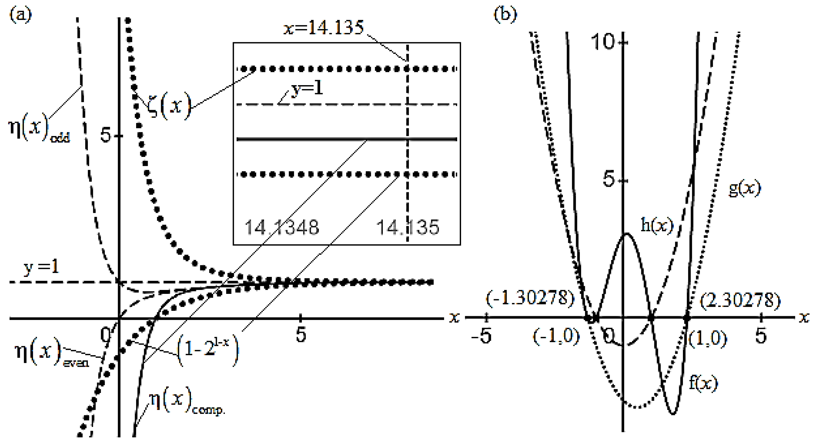
Illustration 1: Since, for, the value of each function is. So, we consider three short forms of the functions and defined as:
, , , and ,
The graphs of functions
,
, and
are shown in
Figure 1 (a). As shown in this figure, for
,
(solid line) and
(point dotted line) are different functions. At an arbitrary point
, still different (graphs shown in inset), but their graphs are far separated parallel lines, that shows, functions
and
never intersect at a point. Thus, the functions
and
cannot have identical zeros.
Illustration 2: Consider a polynomial functiondefined as:, . As shown in Fig. 1(b), graph of product function and factor functionintersects at x-axis, producing two zeros, and function f(x) and intersects at x-axis producing two zeros.
Illustrations-1 and 2 show, when product function and its factor functions are polynomial functions, zeros of product function are identical to the zeros of factor functions [See Fig 1(b)]. However, when one of the factor functions, is a function defined by series, the product function and factor function cannot have identical zeros [See Fig 1(a)].
Auxiliary Theorem II: The conclusion of equivalence of zeros of functions andfrom the definition: is incorrect.
Illustration: We write functions,and define the functions: . Since, for ease, we consider, .The first five -functions are;
,
,
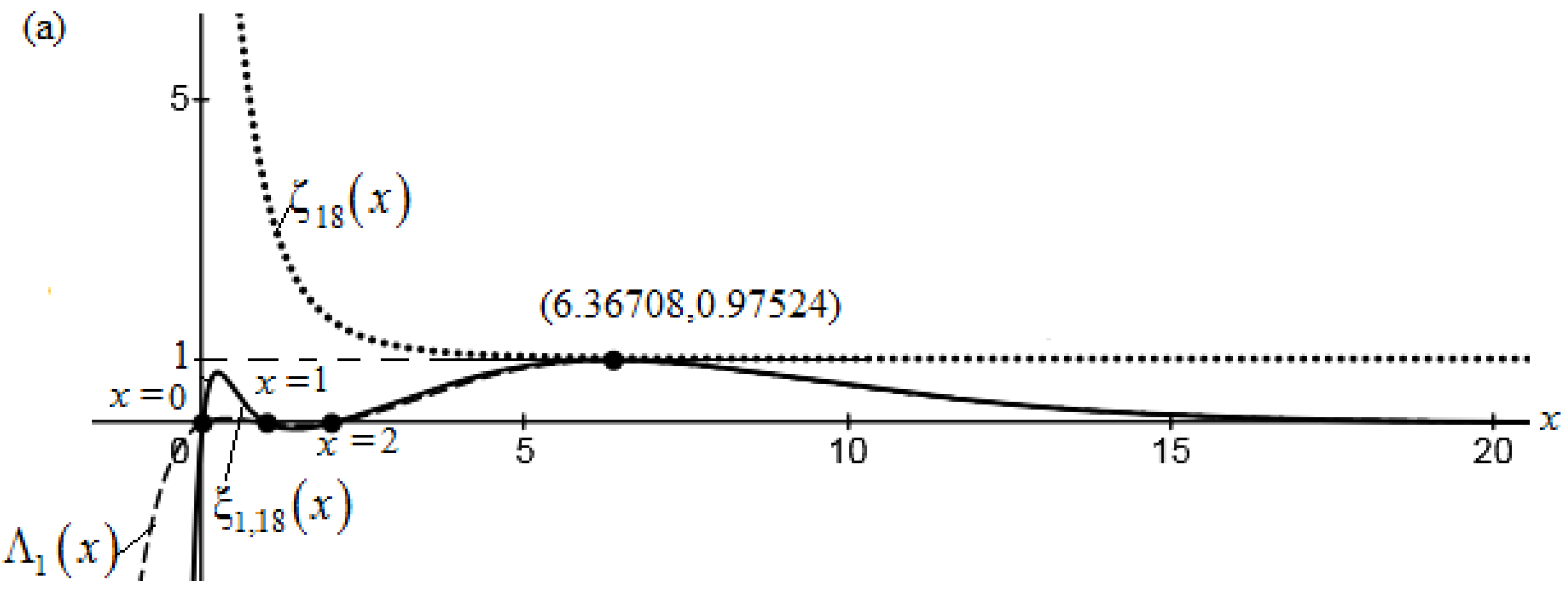
The graphs of product functions and factor functionsand are shown in Fig. 2(a), 2(b), 2(c), and 2(d).
In
Figure 2(a), curves of functions
and
meet at points (6.36708, 0.97524), (0, 0), (1, 0), and (2, 0). These functions have common zero at
x= 0, 1, and 2. However, the graphs of functions
and
nor of functions
and
intersect.
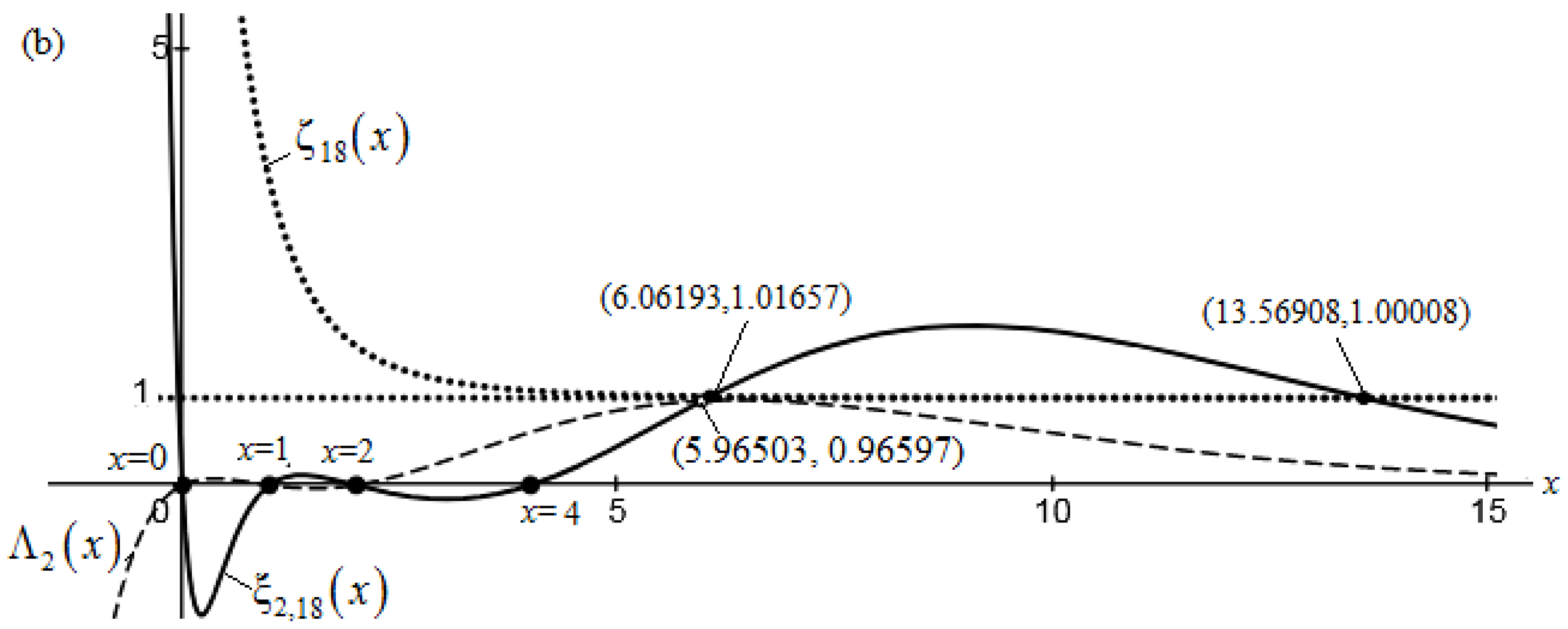
In
Figure 2(b), graphs of functions
and
intersect at points (5.96503, 0.96597), (0,0), (0,1), (0,2), and (0,4), so have common zeros at x=0,1, 2 and 4. Graphs of functions
and
meet at two points (6.06193, 1.01657), (13.56908, 1.00008), but these points do not produce zero/s of either function
or
.
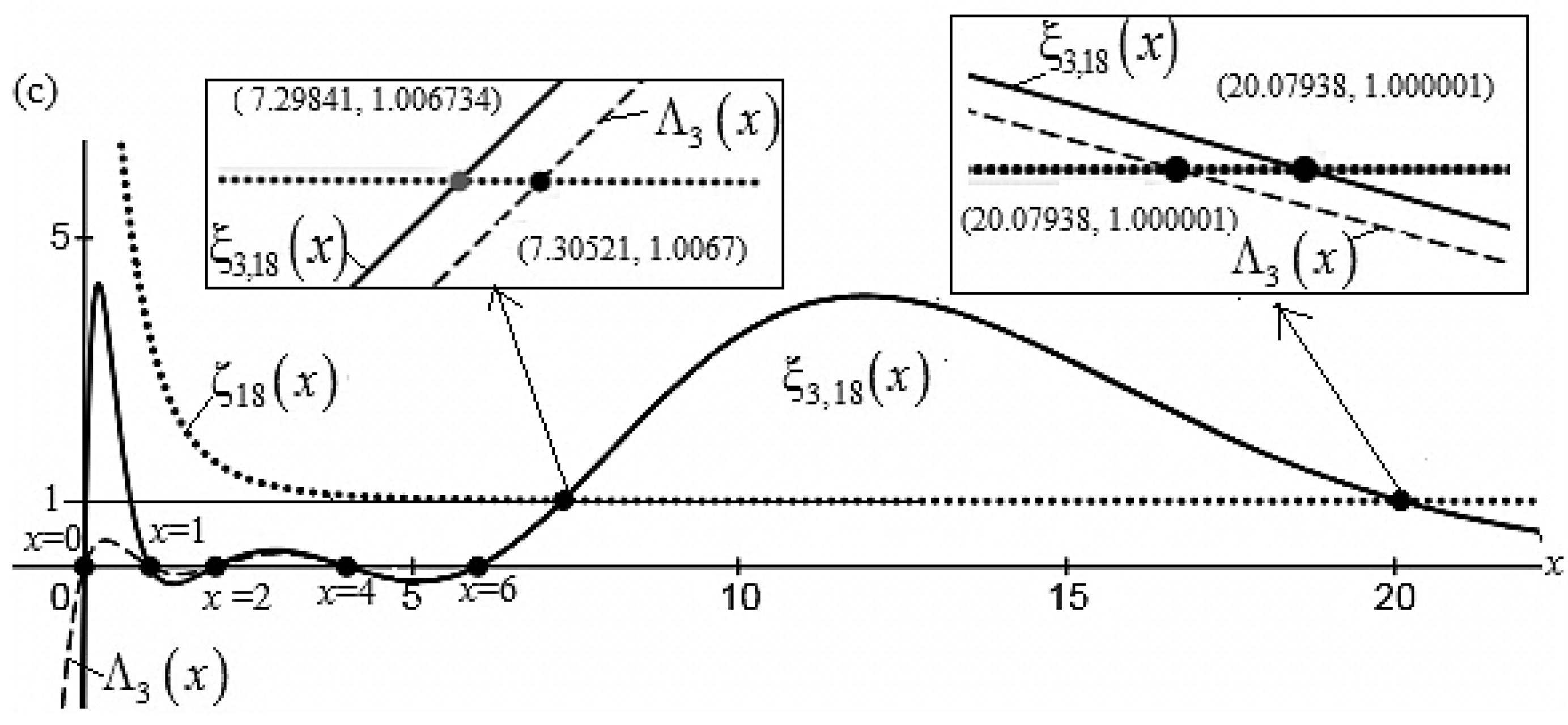
In
Figure 2(c), the number of factors of function
is increased. The functions
and
start overlapping, and the functions
and
share five zeros at
x= 0, 1, 2, 4, and 6. The function
shares points (7.29841, 1.006734), (20.07938, 1.000001 with function
. However, these points do not produce zero/s of either function. The function
shares points (7.30521, 1.0067), and (20.07938, 1.000001), with
but these points are of no use in this study.
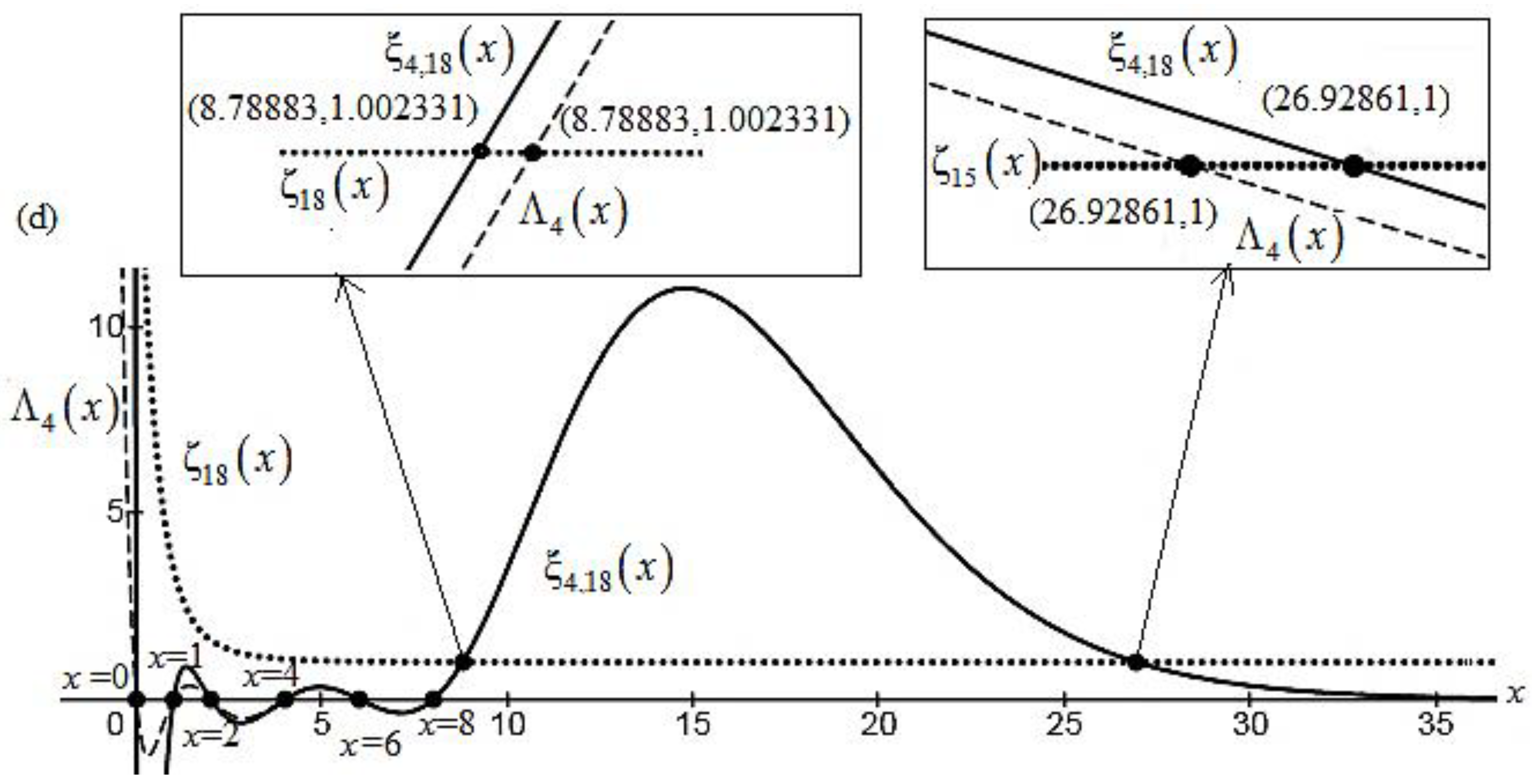
In
Figure 2(d), on increasing the number of factors of function
further, functions
and
overlap and share six zeros at
x= 0, 1, 2, 4, 6 and 8. The combine function of functions
and
shares points (8.78883, 1.002331) and (26.92861, 1) with the function
. That shows the functions
and
may intersect at most at two points on the line
or these functions have only two zeros on the line
.
3. Discussion
The illustrations-1, 2 of auxiliary Theorems I; clearly differentiate behaviors of a product function and its factor functions regarding zeros of the type of functions: (i) when both; the product functions and factor functions are polynomial functions (of real variable) – in this case zeros of factor functions coincide with zeros of product functions. Riemann (1859) used this characteristic of real polynomial functions to the equation to find zeros of function. Later subsequent authors also used to derive the function Z(t). As shown graphically in illustration-1, this application is flawed and so the methods derived from this perception.
Moreover, the function
is the function of complex variable defined by a series that cannot be treated like a polynomial function when verify its zero. For example; if
is a zero of function
, then
; rather,
. Further, the illustration-2 of auxiliary Theorems II, clearly shows that in case of
, if zeros of
and
have identical zeros
(say), then the function
should be a polynomial function, and that could be written as:
. However, function
cannot be written in this factor form because the product on the right do not form a series. Thus, if one assumes that zeros of function
and
are identical, then both function must be polynomials of real or complex variable. Further, the functions
and
can have at most two zeros that lie on the line
. But, the authors listed in
Table 1, have computed zeros count up to
or more. The question is: From where did so many zeros originate? The answer is simple; the methods employed for computing zeros are flawed or since there exist more than two zeros of
, therefore, they (zeros) should be independent of function
or the function
should have different form.
It appears that the certain acceptance of ½ + 14.13472514i, ½ + 21.02203964i, ½ + 25.01085758i, and others as the zeros of functionmight be prompted by fact that the number of computed zeros in certain interval is the same as that predicted by the formula for.
In this article, in Theorem I, II, and illustrations 1, and 2 functions are considered of real variable but results are also valid for variable becausecan be written as.
An interesting outcome of this study: From the illustration of auxiliary Theorem II, an interesting observation leads a new theorem in the “Theory of Functions Defined by a Series.” In the graphs, 2(a) to 2(d), we observe that the graph of product function intersects the graph of factor function at points that lie on a line defined by the denominator of the largest term (here 1/1x) of the function. The line is. If we take this line as the zero-line (or x-axis) for the functions and, that results in a theorem with the statement: “The nontrivial zeros of a function defined by a series always lie on a line” This line likely to be parallel to x- axis or y-axis. Further, investigation is required.
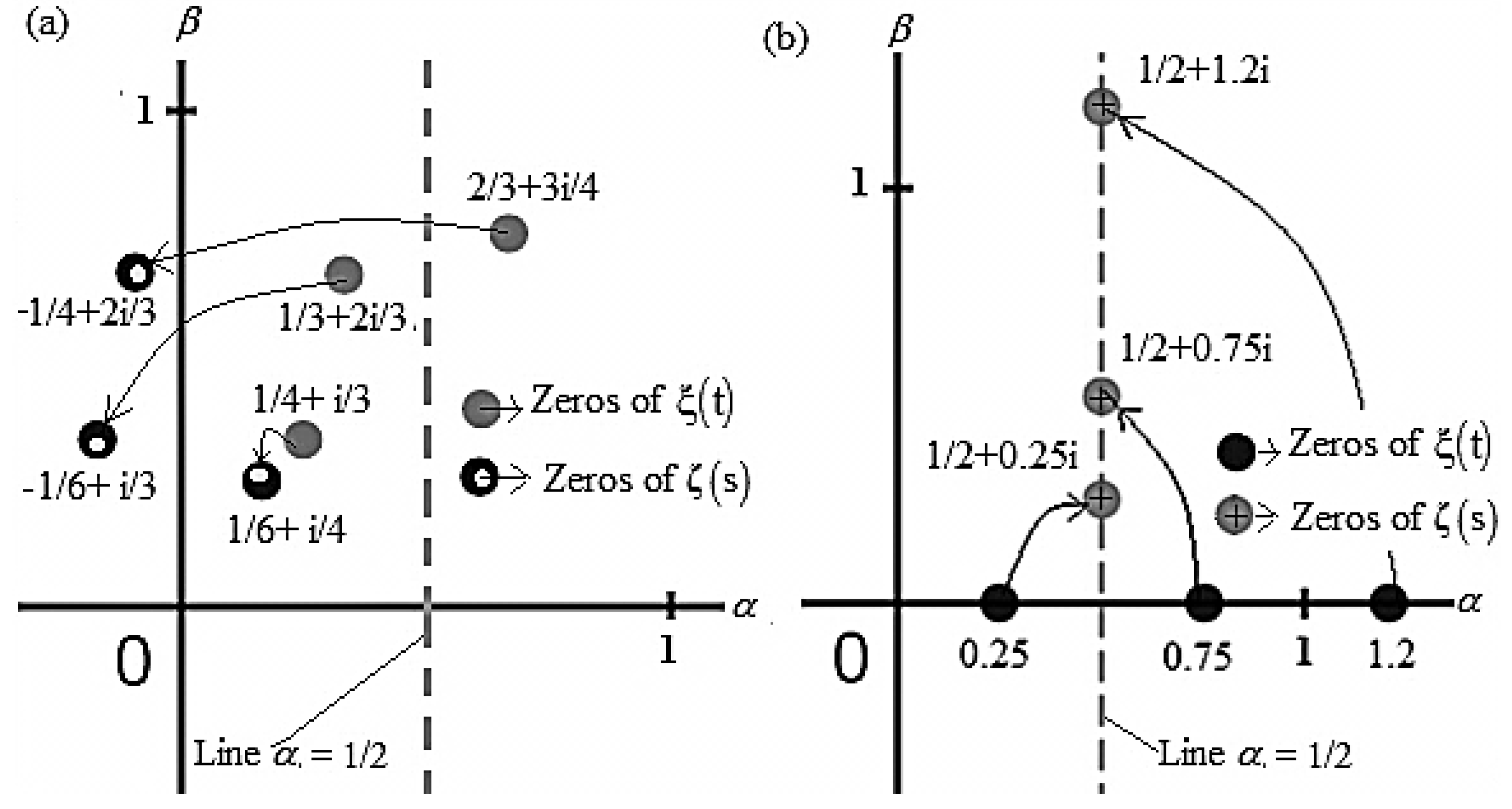
The invalidity of accepted zeros of
has occurred due to misinterpretation of the equation
,
, as discussed above: If one uses the original definition (2) of the function
and calculates zeros of
corresponding to arbitrary zeros of function
, then zeros of functions
and
are not only different but also lie on two mutually perpendicular lines, as shown in
Figure 3(b).
The zeros of functions and shown in Fig. 3 are calculated as: suppose, as the root of. Now, if we assume then. However, the assumptionis invalid as in the illustrations of Theorem I.
4. Conclusion
The methods used for computing nontrivial zeros of functionare derived from assumption that the zeros of functions and are identical. This assumption is incorrect, rendering the methods flawed. Because this assumption forms the basis for the derivation of functionthat is used to compute zeros of by solving the equation, therefore, the widely accepted zeros, such as ½ + 14.13472514i, ½ + 21.02203964i, and others cannot be conclusively accepted as zeros of the function ζ(s). In addition, the validity of the formula , derived under the same assumption, is called into question. The root cause of these issues lies in a misinterpretation of the equation,in which authors consider functions ζ and ξ as the function of same variable. This fundamental oversight in the methodology for computing the nontrivial zeros of ζ(s) could be a significant factor in why the Riemann Hypothesis remains unresolved. Addressing these flaws and reexamining the assumptions underlying Z(t) and N(T) is essential for advancing our understanding of the zeta function and resolving this long-standing conjecture.
Additional Information:
We propose the complex numbers, (1/2 +35.28748i), (1/2 + 51.67246i), (1/2 + 67.98489i), (1/2 + 71.51417i), (78.21896i), and (1/2 +83.77055i) as the only nontrivial zeros of the functionin the interval 0< t <100.
Declaration:
The Author does not have any compelling interest for writing this research article.
References
- Riemann, B. (1859), ber die Anzbahl der Primzahlen unter einer gegebenen Grӧsse Monatsberichte der Berliner Akademie, November 1859, pp. 671.
- Edwards, Harold M. (2001), Riemann’s Zeta Function, Dover ed. (2001).
- Titchmarsh, E.C. The Theory of the Riemann Zeta-Function. OUP ed. (1974).
- H. von Mangoldt, Zur Verteilung der Nullstellen der Riemannschen Funktion ξ(s), Math. Ann. 60 (1905), 1–19.
- Borwein P., Choic S.., Rooney B., Muller A.W. The Riemann Hypothesis- A Resource for the Afficionado and Virtuoso and Alike, CMS Springer-Verlag, P-21, 2008.
- J. P. Gram, Note sur les z´eros de la fonction de Riemann, Acta Math. 27 (1903), 289–304.
- R. Backlund, ¨ Uber die Nullstellen der Riemannschen Zetafunktion. (Swedish), Acta Math. 41 (1918), 345–375. [CrossRef]
- Hutchinson, J. I., On the roots of the Riemann zeta function, Trans. Amer. Math. Soc. 27 (1925), 49–60.
- E. C. Titchmarsh, The zeros of the Riemann zeta-function, Proceedings of the Royal Society of London, A - Mathematical and Physical Sciences, vol. 151, 1935, pp. 234–255.
- Turing A. M. Some calculations of the Riemann zeta-function, Proc. London Math.Soc. (3) 3 (1953), 99–117. [CrossRef]
- Lehmer D. H., On the roots of the Riemann zeta-function, Acta Math. 95 (1956), 291–298. [CrossRef]
- N. A. Meller, Computations connected with the check of Riemann’s Hypothesis. (Russian), Dokl. Akad. Nauk SSSR 123 (1958), 246–248.
- R. S. Lehman, Separation of zeros of the Riemann zeta-function, Math. Comp. 20 (1966), 523–541.
- R. P. Brent, On the zeros of the Riemann zeta function in the critical strip, Mathematics of Computation 33 (1979), no. 148, 1361–1372.
- J. van de Lune, H. J. J. te Riele, and D. T. Winter, On the zeros of the Riemann zeta function in the critical strip. IV, Math. Comp. 46 (1986), no. 174, 667–681.
- X. Gourdon, The 1013 first zeros of the Riemann zeta function and zeros computation at very large height, http://numbers.computation.free.fr/Const ants/Miscellaneouszetazeros1e13-1e24.pdf.
- Platt, D. and Trudgian, J. (2021), The Riemann Hypothesis is True up to 3×10¹². Bulletin of the London Mathematical Society, arXiv: 2004.09765.
- Odlyzko, A. M. The 1020th Zero of the Riemann Zeta Function and 70 Million of Its Neighbors. https://www-users.cse.umn.edu/~odlyzko/.
- Hardy, G. H., & Littlewood, J. E. (1916). Contributions to the theory of the Riemann zeta-function and the theory of the distribution of primes. Acta Mathematica, 41(0), 119–196. [CrossRef]
- C. L. Siegel, ¨ Uber Riemann’s Nachlass zur Analytischen Zahlentheorie, Quellenund Studien zur Geschichte der Math. Astr. Phys. 2 (1932), 275–310.
|
Disclaimer/Publisher’s Note: The statements, opinions and data contained in all publications are solely those of the individual author(s) and contributor(s) and not of MDPI and/or the editor(s). MDPI and/or the editor(s) disclaim responsibility for any injury to people or property resulting from any ideas, methods, instructions or products referred to in the content. |
© 2025 by the authors. Licensee MDPI, Basel, Switzerland. This article is an open access article distributed under the terms and conditions of the Creative Commons Attribution (CC BY) license (http://creativecommons.org/licenses/by/4.0/).