
Submitted:
06 June 2025
Posted:
10 June 2025
You are already at the latest version
Abstract
Coincident changes in abundance and phenology pose a challenge for interpreting abundance indices derived from monitoring programs. In the San Francisco Estuary, long-term monitoring programs have documented changes in overall longfin smelt (Spirinchus thaleichthys) abundance as well as regional differences in presence over time. Seasonal patterns in regional presence of longfin smelt through its life cycle were developed using monitoring data and generalized additive modelling. We investigated the year-to-year variability in seasonal patterns of presence using functional data analysis to separate variability due to population size from variability due to changing timing of presence. We found that longfin smelt have consistent seasonal distribution and that two trawl types were needed to accurately describe those patterns. After accounting for variability due to population abundance, shifts in the timing of presence were evident in three regions. These shifts were interpreted as changes in migration timing. The most variable period for the upstream regions was for age-0 fish in summer and for the downstream region was for age-0 fish in late fall. This study highlights that identifying portions of the life cycle with the most and least variability in distribution can help inform the types of management strategies that will be most effective. It also illustrates an analytical method that can be used to address the problem of confounded effects of abundance and phenology on patterns in monitoring data.
Keywords:
long-term monitoring
; functional data analysis
; endangered species
; osmerids
; environmental change
; geographic distribution
1. Introduction
Ecological monitoring studies generate data on the status of fish species and communities, and they can serve as a context for interpreting trends in abundance and community structure. These “status and trends monitoring programs” provide essential information for decision-makers and ecosystem managers on the state of a system over time (Reynolds et al. 2016). Long-term ecological monitoring can be especially valuable for making inferences about ecosystem dynamics in systems with non-linear relationships between drivers and the variables of interest (Giron-Nava et al. 2017). Even when monitoring studies are designed for status and trends, they can also provide multiple additional values such as quantifying ecosystem responses to environmental change, providing data for developing and testing models, and serving as a framework for collaborative research (Lindenmayer et al. 2012). Monitoring programs may also provide data to evaluate management actions such as flow management, modification or closure of fisheries, or hatchery stocking practices. For this adaptive management approach, timely information about the effect of interventions in the system, is key to evaluating decisions (Allen et al. 2011).
One example of a very long-running status and trends monitoring enterprise is the suite of monitoring studies conducted by the Interagency Ecological Program for the San Francisco Estuary (IEP; IEP 2022). These studies have documented changes in fish abundance in the San Francisco Estuary (SFE) for several decades, including both a substantial loss of pelagic productivity in the late 1980s (Kimmerer and Orsi 1996; Kimmerer 2002) and a collapse in the abundance of several fish species in the early 2000s, a phenomenon referred to as the Pelagic Organism Decline (POD; Sommer et al. 2007). Among the species in decline is the longfin smelt [Spirinchus thaleichthys (Ayres, 1860)]. Once one of the most abundant pelagic fishes in the estuary (Orsi 1999), longfin smelt was likely an important forage fish in the historical SFE. More recently, monitoring programs have documented the decline in longfin smelt abundance and helped identify the factors behind it (Rosenfield and Baxter 2007, Thomson et al. 2010). Freshwater outflow or a suite of correlated variables has long been considered an important factor in longfin smelt abundance in the SFE (Stevens and Miller 1983; Jassby et al. 1995; Kimmerer 2002; Nobriga and Rosenfield 2016; Tamburello et al. 2018), though in the years after the introduction of the overbite clam, Potamocorbula amurensis, declines in the copepod Eurytemora carrolleeae (Alekseev & Souissi, 2011) and the virtual loss of the mysid Neomysis mercedis (Holmes, 1896) as principal food sources had a negative effect on longfin smelt abundance (Kimmerer and Orsi 1996; Orsi and Mecum 1996; Kimmerer 2002; Mac Nally et al. 2010; Thomson et al. 2010). Monitoring data were also used to show that adult stock size also exerts a strong influence on abundance of age-0 longfin smelt (Nobriga and Rosenfield 2016).
The well-documented declines in fish species in the SFE and other bodies of water may reflect more than simply declining abundance. Changing conditions that reduce abundance may also cause species to change the timing of regular movements such as migration patterns. The introduction of the zebra mussel [Dreissena polymorpha (Pallas, 1771)] to the Hudson River estuary led to distributional shifts in young-of-the-year pelagic fishes downstream and young-of-the-year shoreline fishes upstream of the zebra mussel zone (Strayer et al. 2004). Northern anchovy [Engraulis mordax (Girard, 1854)], the dominant planktivore in the SFE, exhibited declines in abundance in upper regions of the estuary after the introduction of the overbite clam and a drastic decline in pelagic productivity within those regions (Kimmerer 2002, 2006); further, because declines did not occur coincidently in the high salinity region of the estuary or the near coastal marine region, they were interpreted as a downstream shift in distribution (Kimmerer 2006). Similarly, a long-term shift by age-0 striped bass from pelagic habitats to shoal habitats was also attributed to declines in pelagic food organisms (Sommer et al. 2011a). Given the long history of change in the SFE, having a flexible spatial distribution in response to changing conditions facilitates stability in recruitment (Colombano et al. 2022).
The potential for coincident changes in abundance and phenology poses an interesting challenge for interpreting abundance data from ecological monitoring programs. For example, assessments of the first appearance of a species may be biased when abundance is unaccounted for because earlier first detections are expected when abundance increases (van Strien et al. 2008). Shifts in distribution or timing of movements might also be interpreted as declines or increases in abundance if sampling only covers a portion of a species’ geographic range or habitats. A variety of methods has been developed to account for this, including hierarchical spatial models (Royle et al. 2007), non-linear spatially-explicit models (Lu et al. 2022), and Gaussian models where spatial coverage is treated as a latent variable (Breivik et al. 2021).
In this paper, we investigate whether there is evidence for changing distribution and movement timing in addition to a decline in abundance for longfin smelt in the long-term monitoring record. In the SFE, longfin smelt abundance is monitored primarily by two long-term, open water monitoring surveys: the Fall Midwater Trawl Survey (FMWT) and the San Francisco Bay Study (Bay Study; Honey et al. 2004; Rosenfield and Baxter 2007). The FMWT samples mid- and upper estuary regions monthly, September through December. Like the FMWT, the Bay Study samples open-water habitats. Unlike the FMWT, the Bay Study samples throughout the range of the longfin smelt within the SFE monthly, year-round and it employs a second gear to sample the bottom, so it may provide a more comprehensive view of longfin smelt use of the SFE (Figure 1).
We developed a statistical model to identify the main temporal patterns in the regional presence of longfin smelt, as detected by the San Francisco Bay Study sampling (CDFW and IEP 2017b). We used this model to examine how the distribution of longfin smelt within the SFE changed over time. The outcome of this modeling is a set of functions that describes the principal seasonal and long-term patterns in distribution by gear, region and age class, which together describe how longfin smelt use the SFE throughout their life cycle. Treating the model output as a set of functions allowed us to separate the effects of abundance from the effects of shifting timing on the probability of observing longfin smelt in different regions of the SFE. We also investigated whether long-term changes in longfin smelt distribution can be attributed solely to changes in abundance or whether there is evidence for changes in the timing of expected patterns in geographic distribution. Finally, we discuss how changes in the timing and distribution of longfin smelt could affect interpretation of abundance trends derived from a less geographically-extensive monitoring program that has historically provided information on longfin smelt.
2. Methods
2.1. Study Species
Longfin smelt is a small (≤150 mm FL), euryhaline, facultatively anadromous, pelagic fish belonging to the family Osmeridae (true smelts). It is native to coastal waters of the eastern Pacific Ocean and bays and estuaries, ranging from Central California to the Gulf of Alaska (Moyle 2002, Moulton 1997, Young et al. 2024). The longfin smelt of the SFE represent the southern-most reproductive population and appear genetically distinct from other populations, although there is evidence of gene flow from the SFE population northward to the Humboldt Bay and Columbia River populations (Garwood 2017; Saglam et al. 2021). Based in part on its precipitous abundance decline, longfin smelt was listed as threatened under the California Endangered Species act in 2009 (OAL 2010) and the San Francisco Bay-Delta Distinct Population Segment of longfin smelt was listed as endangered under the U. S. Endangered Species Act in 2024 (USFWS 2024). Both anadromous and resident populations exist at various locations, and the SFE population is anadromous (Dryfoos 1965; Moulton 1974; Rosenfield and Baxter 2007). The SFE population spawns primarily after its second year of life though some occasionally spawn after their first year and others occasionally live to spawn after a third year of life (≥130 mm collected in winter showing two complete annuli, plus growth; Levi Lewis, University of California Davis, personal communication, Email July 11, 2022). Spawning takes place in or near freshwater sources during the winter and spring (Moyle 2002). Larvae typically hatch from January through April and initially rear in fresh and low salinity water (Dege and Brown 2004, Hobbs et al. 2010, Grimaldo et al. 2017). With further development in the first year of life, they inhabit progressively more saline regions (Baxter 1999). This movement reverses late the following fall and winter when some juvenile fish reoccupy the upper estuary. Second year (age-1) longfin smelt move downstream en masse to marine waters (Central Bay and coastal ocean) during late summer and fall of their second year of life (Rosenfield and Baxter 2007). Finally, during late fall and early winter of their second year, longfin smelt move upstream to tidal fresh and brackish water to spawn (Moyle 2002, Rosenfield and Baxter 2007, Gross et al. 2022).
2.2. Study Area
The SFE is comprised of four, large, open-water embayments (South Bay, Central Bay, San Pablo Bay, and Suisun Bay); the confluence of the Sacramento and San Joaquin rivers, also described as the West Delta; and the Sacramento-San Joaquin Delta, which is a network of tidal channels extending eastward (upstream), and includes remnants of the emergent wetlands that surround these aquatic habitats (Figure 1). The regional descriptors we used were those defined for the Bay Study and except for the West Delta are those also used by Kimmerer (2004). We refer to the embayments and the West Delta as “regions” and “bays” interchangeably when referencing specific embayments within the SFE. Patterns of water flow in the SFE are influenced by climate and human water use factors. Rainfall follows a Mediterranean climate pattern: cold, wet winters and warm, dry summers. This produces highly variable outflows during winter and spring followed by lower, less variable, generally controlled outflows in summer and fall (Arthur et al. 1996). In-flowing river water to the SFE comes mainly from the Sacramento River and tributaries in the north and a lesser amount from the San Joaquin River and tributaries in the south; these inflows meet in the Delta and shift direction to flow west. Net flows (i.e. water not used within the Delta for agriculture or exported south) exit the Delta and defuse successively through Suisun and San Pablo bays, and downstream towards Central Bay and the Golden Gate Bridge, which spans the outlet of the estuary to the Pacific Ocean.
2.3. Data
We used catch data collected by the California Department of Fish and Wildlife’s San Francisco Bay Study (Bay Study) monitoring program (CDFW and IEP 2017b) in our model. The Bay Study sampled fish at fixed sampling locations throughout the estuary once per month, year-round. At each sampling location, the Bay Study collected fish using two different gears: an otter trawl (OT) and a midwater trawl (MWT). Both net types were deployed to the bottom; the OT skimmed the bottom for its tow duration, whereas the MWT was retrieved obliquely to collect an integrated sample throughout the water column. We used data from Bay Study’s series 1 and series 2 sites. Series 1 comprises the original 35 stations which have a variety of depths, but depths > 7 m predominate. Series 2 includes seven additional shoal stations with depths of 2-6 m, which were added in 1986 to more evenly balance channel and shoal stations across regions. Although the record is longer for Series 1, we only used data from 1986 – 2015 from both series. Data from this set of years allowed us to follow 28 year-classes through approximately 36 months, near their putative maximum life-cycle duration. Beginning in 2016, the Bay Study experienced a protracted period of missed samples by one or both gear types, so we did not use more recent data. The Bay Study measured a representative sample of up to 50 fish per species, per net tow, per station to the nearest mm fork-length (FL) and counted the remainder. When more than 50 longfin smelt were caught in a single tow, the length distribution of the 50 individuals measured was applied to the entire sample (Rosenfield and Baxter 2007). Age classes were assigned to individual longfin smelt based on length (Table 1). The minimum length for inclusion was 40 mm FL and this became the minimum size used in our presence analyses; thus, initial detections described in this study began in the months when and in the regions where longfin smelt first attained 40 mm FL.
For our study, we needed to track and describe regional presence of each year-class continuously through its life cycle. To accomplish this, we further processed the Bay Study’s count data to obtain presence or absence of longfin smelt for each gear type at each individual sampling station (3 – 11 stations per region) for each age-class (Figure 1). This produced a binary dataset of presence/absence records for each combination of site, month, gear, and age-class. We assumed that all fish of a year class hatched in January (longfin smelt predominantly hatch in winter; Baxter 1999) and thus January represented month 1 for each new year-class and subsequent months in sequence were used to describe rough age progression through 36 months of tracking, though not all year classes were detected through 36 months. We used these consecutive monthly designations to track each year-class through each age class to facilitate modeling, inter-year-class comparisons, and for descriptive purposes (i.e., sequential age and month numerals align among year classes). We do not intend our monthly designations as exact ages per-se, but as age approximations to describe how each age class was distributed and responds to its environment in each month.
Age class records were labeled by year-class year, which we defined as the year when fish were detected as age-0 fish, to facilitate consistent predictions across subsequent calendar years as fish increment ages. This prevented jumps in predicted probability of catch from December to January and it allowed the model to account for different patterns in movement for different life stages. Months were also labeled consecutively through the life cycle to reflect potentially changing distribution of the age classes through time (age-0: months 1-12; age-1: 13-24, age-2+: 25-36). Presence/absence data from individual stations for the two gears were used in the models, rather than aggregated values for regions. This provides some variability in the presence or absence of longfin smelt in the samples within each month so that a seasonal trend can be evaluated for each region.
In addition to understanding patterns in the Bay Study time series, we used our modeling results to interpret patterns in the annual abundance indices for longfin smelt derived from a second monitoring program, the FMWT. The FMWT is among the longest running monitoring studies in the SFE (Honey et al. 2004), and it provides the commonly cited indices for species abundance. Like Bay Study, FMWT index values are assumed to provide a relative approximation of population trends over time; however, the geographic scope of the FMWT is less extensive in the lower SFE compared to that of the Bay Study (Figure 1). We examine how shifts in patterns of seasonal timing uncovered using data from the Bay Study might influence FMWT index values. The FMWT samples stations range from western San Pablo Bay upstream through Suisun Bay and part of Suisun Marsh and throughout the Sacramento-San Joaquin Delta monthly from September through December (Rosenfield and Baxter 2007). The annual FMWT abundance index is calculated as the sum of September through December monthly indices; monthly indices are calculated as the sum of the products of mean regional catch per tow and the respective regional weighting factors (Rosenfield and Baxter 2007; CDFW and IEP 2017a).
2.4. Modeling Distribution
The probability that longfin smelt are present in each gear type at each sampling month and region was modeled using a Generalized Additive Model (GAM) with a logit link. A GAM for probability of presence is similar to a logistic regression model, but with additional flexibility. The probability of presence was fitted as a function of a life-span trend (month, over 36-month life span), long-term trend (year, age-0 for 28 individual year-classes) and the change in life-span trends over time (interaction of month and year) and each of these three terms was allowed to vary by region and gear type. We defined “month” as the month of life of longfin smelt so life-span trends are fit over 36 months. We defined “year” as the brood year (or year class), so there are 30 years in the model, representing 28 full life cycles during 1986-2015. Additional parametric intercept terms were added to the model to account for differences between the gear types in each region (interaction of gear and region and the associated main effects).
All analyses were conducted using R (version 4.3.1; R Core Team 2023). GAMs were fitted using the gam function in package mgcv (version 1.8-16; Wood 2011). Smooths were fitted using thin-plate regression splines (Wood 2003), and tensor products (Wood 2006). The model included smooths for the long-term and seasonal trends in presence. The purpose of this model is to create a set of functions that describe the probability of longfin smelt use of specific regions. To accomplish this, the model needed to be formulated in a way that the resulting functions capture the major features of the long-term and life-span trends without introducing shorter-term fluctuations that might be expected from environmental variations. We plan to examine the effects of environmental variation on longfin smelt presence in a future analysis. Thus, we limited the degrees of freedom for our smooth terms in these models to avoid over-fitting. It could be tempting to increase the number of degrees of freedom to account for more of the variability in the data, but the improved fit would artificially attribute the patterns caused by other factors (e.g., environmental variables) to the temporal trends. In other words, our model at this stage was not intended to explain the maximum possible variability in timing, but instead describe broad patterns in distribution and major trends in timing. Following advice in Fewster et al. (2000) for how to choose an appropriate level of smoothing, we plotted the smooth terms for month and year class over time, shared across gear types, with various numbers for the maximum allowed knots (k). We found that when k was approximately equal to 0.3 times the number of x values, the resulting smooths produced a time series that described the major features of the data without adding excess wiggliness (Pedersen et al. 2019), or complexity contributed by other drivers rather than the temporal patterns of interest, to the trends.
We recognize that readers expect the “best” model to be the one with the lowest AIC value; however, AIC is not the best tool for model selection in this case because the criteria for optimization in the AIC calculation are not consistent with the objectives of our modeling exercise. Specifically, there is a mismatch between the level of wiggliness that is acceptable for our purposes of analyzing trends and the way AIC selects optimal wiggliness. In fact, Fewster et al. (2000) advise against the use of automatic selection procedures such as AIC in trend analysis for this reason. Similarly, Pedersen et al. (2019) recommend using subject expert knowledge about the system and the goals of the particular study for model formulation and selection rather than relying on AIC to select a best generalized additive model because multiple model structures may fit the data similarly, but some structures may not be appropriate to answer the questions of interest.
2.5. Functional Data Analysis
Functional Data Analysis (FDA) comprises a suite of techniques for extracting information about values that vary smoothly over a continuum. These functions could take the form of a curve that varies along one explanatory variable or a surface that varies with the combined effects of two explanatory variables. The predicted probabilities that are generated by the GAM are a type of functional data. The predicted probabilities for each region vary on two temporal dimensions and we can generate smooth curves to show how the probability of presence varies on a seasonal scale or the long-term scale across years. We used the function fdata (package fda.usc; Febrero-Bande and de la Fuente 2012) to convert the predicted probabilities into functional data objects that could be analyzed under the FDA framework.
The characteristics of the shape of the life-span curve provide information about when longfin smelt are most likely to occupy a particular region during their life span. Months with higher probability indicate times during the life cycle when longfin smelt most use a particular region. The width of the peak indicates how long longfin smelt reside in that region. The mean pattern of longfin smelt presence is of interest for quantitatively depicting how the species uses the SFE. When and where variation occurs from the mean pattern is also of interest because that could indicate changes in patterns of presence, such as a shift from a historical pattern to a modern pattern.
The probability of detecting longfin smelt in a region at a particular month varies from year to year. Using a functional data analysis framework, the ways each year-class-specific curve differs from the mean can be broken into two components: amplitude variation and phase variation. Amplitude variation is the variability in the height of the curves (i.e., a deformation in the y-direction; here related to abundance); in this case it represents variation in the magnitude of the probability that a longfin smelt is caught. Phase variation is the lateral displacements or deformation of curves that are not explained by variability in amplitude (i.e., deformation in the x-direction; here related to timing). In the case of predicted probabilities of longfin smelt presence, phase variation indicates a shift in presence to earlier or later in the life cycle (in months).
To determine a mean pattern for reference, the curves for predicted probabilities of individual year-classes needed to be aligned and a functional average calculated. To align two curves, a “warping function” transformed the curves to make them as similar as possible. Aligning curves decouples phase and amplitude variability without losing information because the warping function contains the phase variability, and the amplitude variability is the variability that remains (Sangalli et al. 2010). The aligned functions were then averaged to produce a curve that describes the expected pattern of presence for each region. The amplitude variability provided information about how consistent the expected seasonal pattern was from year to year and values of the warping functions at each month provide information about whether there had been a directional shift over time. We used the function time_warping (package fdasrvf; Tucker 2017) to align the life-span curves for each region and produce a functional average. The time_warping procedure aligned functions using the elastic square-root slope framework. We provide the relative values of amplitude and phase variance by region and gear type to show the major sources of variation.
To identify timing shifts in regional presence, we first plotted phase variance by month through the life cycle for each gear type (28 year classes where each year-class contains 36 months of regional presence data from 2 gear types) and identified the month of peak variance and noted variance of proximal months. We then plotted values from the warping functions for these peak months separately by gear type to look for consistent, directional shifts over time. We chose to only plot functions from months with the peak variability. Adjacent months showed the same directional change but lesser magnitude (see variability results); thus, supporting the same response to a lesser degree.
3. Results
3.1. Smoothing (GAMs)
We found significant parametric effects of bay and gear type as well as their interaction (Table 2). The model with the optimal levels of smoothing to meet the goals of the study had 11 knots for the life-span trend and 9 knots for the long-term trend (Figure 2). These values allowed the relationship between probability of catching longfin smelt and the two trends in time to capture the major features of the relationships without overfitting. The equation for the optimal model was
where each terms represent a distinct set of smooth functions, with k knots, and where terms represent parametric intercepts for two gears (i) and five regions (j). The optimal model explained slightly less than one third of the variability in the presence/absence data (deviance explained = 26.8%).
Smooths for the long-term trends indicated that the probability of catching longfin smelt fluctuated over the long-term, but the trend was overwhelmingly decreasing for all regions since the late 1990s (Figure 2; graphs for other bays are in Supplemental Materials).
3.2. Functional Data Analysis
General features of the mean probability curves – Mean functions for the predicted probability of longfin smelt presence depicted when longfin smelt are most likely to be observed in each region over the course of the life cycle (Figure 3). The difference between the gears was largely spatial. The OT generally predicted greater presence downstream (e.g., Central Bay) and the MWT predicted greater presence upstream (e.g., Suisun Bay, Figure 3). The gear types agreed on the general timing of presence. This was particularly evident for the expectation of broad distribution during winters and relative absence during late summers (i.e., August, month 20). For both gears, probability of presence peaked in winter at the end of the first year of life (Dec or Jan; months 12-13) in all bays except Central Bay, which peaked in summer (July, month 7) in both gears (Figure 3). An earlier, lesser peak also occurred in San Pablo Bay in summer (July, month 7) for both gears; though of different magnitude, this peak closely matched that of Central Bay timing-wise. Other, lesser peaks occurred the following winter (December- February, months 24-26). There are three major nadirs in probability of observing longfin smelt. The probability of observing longfin smelt was essentially zero for months 1-3 because at this age longfin smelt were too small to be reliably retained by the sampling gears (and were mostly below the minimum length and not counted). The second nadir occurred in the summer of their age-1 year, around months 19-22 (Figure 3). This is the time during the life cycle when longfin smelt spend time in marine conditions (primarily, Central Bay and coastal ocean) so their range within the SFE is small during this period. The third nadir was in summer of their age-2 year, around months 27 – 34 (Figure 3). Similar to age-1 fish, age-2 fish are in marine waters at this time. San Pablo Bay and the West Delta exhibited small increases again at months 35 & 36.
Variability – The pattern and height of regional peaks across years of study corresponded to changes in population indices from monitoring programs. Specifically, the relatively high abundance in the late 1980s and late 1990s and the subsequent decline that was apparent in FMWT indices (Figure 4) was also reflected in the long-term probability of catching longfin smelt from the model (Figure 2, right column panel where k = 9). There was considerable variability in the timing of presence for age-0 longfin smelt in summer and fall in both Suisun Bay and the West Delta (Figure 5 & Figure 6). In fact, the phase variance (i.e., variability in timing/magnitude of presence) was distinctly higher in Suisun Bay and the West Delta relative to other regions (Table 3). Higher phase variance indicates that the observed timing of presence in these regions was more variable than other regions after accounting for the influence of fish abundance on the height of the curve (i.e., amplitude variance).
The values of the warping functions showed the months when the patterns in cohorts deviated from the mean life-span functions in ways that cannot be accounted for by changes in abundance alone (Figure 5 & Figure 6). For both gear types, the mean probability curves for South SF Bay were perfectly aligned for all years because the interaction term for lifespan and year was not significant for that region. Central SF Bay, Suisun Bay, and the West Delta all had clear peaks in phase variation relatively early in the life cycle. For the West Delta and Suisun Bay, the peak in phase variation was in the summer (Jun-Jul, months 6-7) and fall (Aug, month 8) of the age-0 year, respectively. For Central SF Bay, the peak in phase variation was in winter around months 12 and 13. Lesser amounts of phase variation were also evident in the upper estuary (Suisun Bay and the West Delta) in later months of the life cycle.
The timing and direction of phase shifts was investigated for months with the highest phase variability, and the temporal shift patterns were plotted relative to those peak variance months for each gear and region (Figure 7). The West Delta had the highest variance and shifts in timing of age-0 summer (month 7 for MWT, month 7 for OT) presence. The shift in timing gradually changed from two months earlier than average to two and a half months later than average over the course of the time series. The shift from around average timing to later happened rapidly from about 2005 to 2015 (MWT) and 2008 to 2014 (OT; Figure 7). The highest variance in presence, and thus shifts in timing of presence, in Suisun Bay occurred during the age-0 summer (month 8 for MWT, month 8 for OT) varied from two months earlier to two months later than the mean function (Figure 7). Major shifts in timing occurred in the mid- to late-1990s, when the direction changed from later than average to earlier than average, and in the mid-2000s, when the pattern reversed.
For the Central Bay, peaks in variance in the winter (month 13 for MWT, month 12 for OT) provided evidence of shifts in timing for age-0 longfin smelt. The amount of phase variation for Central Bay was much higher in the OT than for the MWT. Through the mid-1990s, longfin smelt MWT-based presence in Central Bay shifted from later than average to earlier by 1996 and this shift to earlier timing was maintained through the end of the study period (Figure 7). Similarly, OT-based presence in Central Bay in December shifted from 2.5 months later in 1987 to one month earlier by 2000, where it remained (Figure 7). These three examples represented the maximum variances identified among several months of increased variances for each region and gear identified; patterns of shifts for those increased-variance months not shown generally matched those that were shown.
Patterns in the monthly index values for the FMWT reflected shifts in timing of fall movements, as indicated by the functional data analysis of the SFBS data (cf. Figure 4 and Figure 7). Specifically, the September index values were low when the August pattern for Suisun Bay is later than average (Figure 7). During the period when the August pattern for Suisun Bay was earlier than average, the monthly FMWT index values appeared to be higher in general, and the September index values tended to account for a larger proportion of the total index.
4. Discussion
We developed foundational models that describe how an important endangered forage fish, the longfin smelt, occupies regions of the SFE both monthly year-round and throughout its life cycle. Such models can be developed elsewhere when the resolution of fish monitoring data is seasonally and geographically sufficient to provide input for model fitting. It is also flexible, incorporating data from more than one gear type targeting the same life stage(s) of interest. These models support describing consistency in geographic distribution and timing of presence, as well as variation from the expected pattern. We found that phenological patterns were more variable in the youngest longfin smelt in our dataset, whose distribution are most influenced by hydrology, but there was evidence of subtle shifts in the timing of movements throughout the age-0 year. We believe that our methods could benefit other fish monitoring enterprises by documenting stable and any shifting timing of regional habitat use through the portion of life history captured by the monitoring program. The results of these models can be used by fishery managers and regional planners to identify seasonal periods of expected high or low presence for migratory fish. This information can help to determine when and where habitat restoration might have the greatest benefit or to identify periods of relative absence in which to schedule in-water projects to minimize negative effects (e.g., channel dredging, piling installation).
4.1. Abundance-Related Variation
The pattern of decreasing probability of capture in every region over the long-term (i.e., across years) reflects declining abundance of longfin smelt in the SFE (Rosenfield and Baxter 2007; Sommer et al. 2007; Thomson et al. 2010; Hobbs et al. 2017). Variation in regional probability of presence also reflects events in life history. Regional patterns in presence of longfin smelt in the SFE over their lifespan were relatively consistent over time; the mean predictions depict the general patterns of how longfin smelt seasonally use the regions of the SFE.
Patterns in probability of catching longfin smelt indicated that age-0 longfin smelt move downstream in substantial numbers during the first six months of their life cycle and began to recruit to the Bay Study sampling gear about two thirds of the way through that period. Recruitment to the gear likely occurred fully in their first fall through winter, based on retention of delta smelt [Hypomesus transpacificus (McAllister, 1963)] and its similar but slightly thicker body shape at length compared to longfin smelt (Mitchell et al. 2017). Many returned to the upper estuary in fall and winter (months 9-13) before again moving downstream toward the Golden Gate (months 14-17) and spent the summer in the ocean (months 18-20). Beginning in fall, they repeated the cycle of moving up estuary, this time for most to spawn (months 22-26) and for those that survive, back down again (months 27-29). Finally, in their third fall, those few surviving at the end of their third year repeated the cycle moving up estuary to spawn (months 34-36).
These movements resulted in a consistent cyclic pattern of broad distribution during the cooler months of the year followed by a more compressed distribution (i.e., Suisun Bay to Central Bay, and the open coast) during the warmer months. The broad geographic distribution of longfin smelt occurs during the winter and spring spawning (months 24-27) and early rearing (months 1-5) periods that includes South Bay, particularly during high rainfall years (Baxter 1999, Lewis et al. 2020) as well as the mid- and upper SFE. As the summer progresses (months 7-8), South Bay and the West Delta are rarely if ever occupied (Baxter 1999), likely due to increasing water temperatures (>20°C, see Jeffries et al. 2016). However, as water temperatures decline in fall, both South Bay and the West Delta are once again habitat for both juvenile (months 11-13) and putatively mature (months 23-26) longfin smelt. Our model results support the consensus that that longfin smelt in the SFE are anadromous, but they also provide evidence that beginning at age 0, but more commonly at age 1, they spend the summer months outside the SFE in the coastal ocean and in cool marine salinities in Central Bay (Rosenfield and Baxter 2007, CDFG 2009, Garwood 2017). The estuary-wide declines in probability of capture that occurred during the summer (months 15-21, 27-31) cannot be attributed to mortality alone because probabilities increased again in the subsequent fall months. Natural mortality resulting in a lower seasonal presence of age-1 longfin smelt in the estuary in their second fall and winter (Figure 3, cf. months 22-28 with months 10-16) contributed to a lack of substantial phase variability during that period. Nobriga and Rosenfield (2016) detected declines in survival of juvenile longfin smelt over time based on abundance ratios that also confirmed this decline in seasonal presence.
The early life stage patterns and variation in regional presence reflect a combination of contemporaneous and preceding factors, namely recruitment to the sampling gear and movement, respectively. The initial slopes (i.e., months 4-11) in the regional probability of presence curves are explained to a large extent by recruitment to the gear, which in this case begins when fish reach 40 mm and are counted. Substantial hydrodynamic and volitional movement of longfin smelt larvae and juveniles occurs prior to recruitment to the gear. Spatial distribution varies most for longfin smelt larvae and small juveniles because their location is dependent upon freshwater outflow in the winter and spring (e.g. Dege and Brown 2004, Grimaldo et al. 2020, Gross et al. 2022). Although our analysis cannot directly assess the timing of larval movement, our results show a consistent pattern of downstream recruitment in San Pablo and Central Bays by the time fish reach 40 mm (the minimum size counted from the sampling gear) in both high and low outflow years. Freshwater outflow influences upper estuary circulation patterns (Kimmerer 2004) and thus the distribution of larvae (Baxter 1999; Dege and Brown 2004, Grimaldo et al. 2020). Although Longfin Smelt larvae show a predominant surface orientation immediately after hatching and improving competency for vertical migration with airbladder development weeks later at 10-12 mm (Bennett et al. 2002, Hobbs et al. 2006) they nonetheless possess the ability to maintain favorable position in the low salinity zone of the SFE (Dege and Brown 2004, Hobbs et al. 2010), though larvae remain common to salinities of 10-12 psu (Grimaldo et al. 2017). Larvae in other systems also make use of a combination of limited swimming abilities and hydrodynamic circumstances to place and maintain themselves in favorable low salinity, often high turbidity, nursery habitats soon after hatching (Dodson et al. 1989, Laprise and Dodson 1989, Bradbury et al. 2006, North and Houde 2006, Couillard et al. 2017). In high outflow years substantial numbers of longfin smelt larvae and small juveniles in the SFE are distributed into San Pablo Bay and occasionally beyond; in low outflow years, most larvae are initially found in Suisun Bay and upstream (Baxter 1999; Dege and Brown 2004, Grimaldo et al. 2020, Gross et al. 2022). Regardless of outflow magnitude, age-0 fish tend to initially recruit to Bay Study trawl gear downstream first as reflected by the earliest increases in predicted probabilities in San Pablo Bay for both gears and Central Bay for the OT increasing prior to those of upstream regions. This pattern is likely at least partially a result of aggregated effects of outflow in some years on larvae, but also reflects substantial volitional downstream movements of late-stage larvae and small juveniles (ontogenetic migration) prior to capture.
4.2. Variability in Timing
While the functional averages of the aligned annual curves by age class provide a description of the expected patterns in life history, our functional data approach uncovered additional information about the life history of longfin smelt in the variation around these expected patterns. We found that changes in the annual distribution of longfin smelt in the Estuary reflect differences in timing as well as declining abundance. Some periods of the life cycle were more variable than others in terms of distribution and timing. The most pronounced changes in the life-span pattern of presence over time occurred during mid- to late age-0 and early age-1 in Central Bay, Suisun Bay, and the West Delta. These periods may be important for understanding when longfin smelt react to a changing environment and for deciding when management actions may have the most impact on longfin smelt. Such changes in distribution timing may also influence our interpretation of existing abundance indices. The ways individual year-classes of longfin smelt deviate from the mean probability function provide insights into changes in the seasonal distribution of longfin smelt in the SFE. After accounting for changes in abundance, changes in the seasonal patterns in regional probability of presence reflect measurable changes in timing of movements for longfin smelt. Movements in younger life stages that oscillates downstream and upstream with the position of habitat with favorable salinity, as described above, contributed to phase variation for earlier life stages because the timing of their presence in some regions is dependent hydrodynamics. Directional phase shifts of presence over time indicate that longfin smelt have changed the timing of their movements among regions as well as into and out of the estuary. These changes in distribution likely reflect large-scale changes in environmental factors (e.g., water temperature) as well as changes in habitat suitability with ontogeny (e.g., salinity tolerance increases) that also follow predictable seasonal patterns.
For example, longfin smelt appear to spend more time farther downstream and in the coastal ocean in recent years than they did historically. The summer to fall pattern of presence for the age-0 longfin smelt in the West Delta shifted steadily later from the mid-1980s to 2015 and the patterns that are expected during the winter in Central Bay have shifted three to four months earlier than what was observed in the late 1980s. During the age-0 fall and age-1 winter, longfin smelt are well-distributed throughout the estuary after few summer detections in the West Delta and South Bay (months 7-8, 19-20) and after some likely returned to the estuary from the ocean. From 2000 – 2015, the modest pattern of presence in the Central Bay in the early winter has shifted steadily earlier in the year, reflecting a steep decline in seasonal use of Central Bay or more rapid movement through the Bay during the winter. This suggests that longfin smelt moving upstream in the fall and winter do not use Central Bay as much during the winter as they had in the past and that some may choose to instead remain in the ocean for another year until they make their migration to spawning areas upstream. The variability in the timing of longfin smelt use of Central Bay may reflect an overall variability in use between the marine habitats of Central Bay and the coastal ocean. The dataset we used does not sample the coastal ocean, but this directional change supports the idea that longfin smelt remain in the ocean longer and avoid spending time in the Central Bay as juveniles (months 12-14).
High water temperatures are also likely to be a major factor that limits the upper estuary (Mahardja et al. 2022) and South Bay distributions of age-0 longfin smelt during summer and fall. Longfin smelt larvae showed signs of heat stress at 20°C (Jeffries et al. 2016). Juveniles were present in 20-22°C, but were not repeatedly caught in 22°C water (CDFW unpublished), so 20-22°C is considered high water temperature. The probability of presence for the West Delta was typically low in summer (months 7-8) and a rebound from that low shifted roughly 2 months later than average through the study period. In Suisun Bay during summer and fall, detections typically were modest at best (months 8-9) and increases beyond these modest detections oscillated from later than average to earlier and back to later. The earlier timings in the mid-1990s to mid-2000s coincide with a period of relatively high abundance values and a period of numerous relatively high outflow years. Wet winters and springs coincide with favorable temperature conditions in early summer and late fall (Bashevkin and Mahardja 2022) that, in turn, result in increased probability of presence for Suisun Bay earlier in the fall than occurs on average. During the summer and fall, Delta outflows are typically low for the SFE (Kimmerer 2004), and it is common for temperatures to approach and exceed thermal maxima for longfin smelt (Jeffries et al. 2016), especially in the upper estuary and South San Francisco Bay. In South Bay, larvae and small juveniles are observed in high rainfall years (Baxter 1999, Lewis et al. 2020), yet by mid-summer and early fall detections are essentially zero until about November (month 11, Figure 3). This likely indicates that South Bay is only seasonal habitat. In the future, the SFE faces warmer and drier conditions in summer and fall (Knowles et al. 2018) that may further reduce the period of the year when conditions in South Bay, Suisun Bay and the West Delta are favorable for longfin smelt.
Longfin smelt is not the only species to exhibit changes in distribution within the SFE in response to changing conditions. In the late 1980s northern anchovy shifted downstream out of the upper estuary (Kimmerer 2006) and at about the same time, age-0 Striped Bass shifted away from pelagic habitats to the shoals (Sommer et al. 2011a). In both instances the shifts were interpreted as responses to a sharp decline in pelagic productivity after the introduction of the overbite clam [Potamocorbula amurensis (Schrenck, 1861)]. Fishes in the Sacramento-San Joaquin Delta have also responded to an increase in water exports and fish entrainment from the south Delta in the late 1960s (Arthur et al. 1996, Grimaldo et al. 2009) and subsequent increasing south Delta water clarity, and proliferation of invasive submerged aquatic plants and introduced fishes (Brown and Michniuk 2007, Nobriga et al. 2008). For example, the endemic delta smelt no longer rears in the south Delta (i.e., San Joaquin region, Nobriga et al. 2008) and threadfin shad [Dorosoma petenense (Günther, 1867)] numbers have declined sharply in the region (Feyrer et al. 2009). In contrast, fishes associated with vegetation and the shoreline, particularly introduced Centrarchids, have increased in response to an increase in vegetated habitat (Mahardja et al. 2017). Similarly, on the eastern US coast, community-wide distributional shifts by fishes have also been documented in the Hudson River Estuary after the introduction of the zebra mussel [Dreissena polymorpha (Pallas, 1771)] and its feeding on phytoplankton and small zooplankton changed pelagic food availability in that system. Young-of-the-year pelagic fishes (e.g., Morone spp. and Alosa spp.) shifted their distribution downstream whereas young-of-the-year shoreline fishes (e.g., Centrarchids and Killifish) shifted upstream of the zebra mussel zone (Strayer et al. 2004). Numerous other factors have been reported to contribute to these shifts (Daniels et al. 2005).
4.3. Implications for Interpretation of Abundance Trends
Modeling regional presence allowed us to identify and track when altered presence timing indicated substantial movements into or out of the geographic sampling frame and provided a means to distinguish a shift in distribution from a change in abundance. Such information helps avoid potential misinterpretation. An example for the SFE is the FMWT, which samples from San Pablo Bay upstream through the Delta. Even with incomplete geographic coverage of LFS distribution in the SFE during the fall (i.e., no sampling in Central or South San Francisco bays), the FMWT abundance index tracks the general decline in longfin smelt abundance (Rosenfield and Baxter 2007, Thomson et al. 2010).
Understanding the distribution of fish and the phenology of their movements can improve interpretation of their population trajectories as described by abundance indices. Later fall migration to Suisun Bay and the West Delta would appear as a reduction in FMWT longfin smelt abundance beyond that of an already declining population. This delay is evident from the different relative magnitudes in the monthly indices in over time; in particular, September indices make up a lower proportion of the total FMWT index in the earliest (ca 1988-1994) and latest (2005+) years than they did in the late 1990s and early 2000s. This indicates that age-0 longfin smelt partially resided downstream of the FMWT sampling regions for the first part of the annual survey. It is not clear whether presence increased later in the sampling period compensating for the absence early in the sampling period, but patterns of presence indicate that age-0 and age-1 longfin smelt returning in fall and early winter remain in upstream regions throughout the winter and early spring, and similarly, providing repeated opportunities for capture of each age class. A similar pattern has been observed in other species whose distribution is influenced by changing environmental conditions. For example, the movement phenology of yellowfin sole [Limanda apera (Pallas, 1814)] in the Bering Sea has changed over time, causing different proportions of the population to be available for biomass estimation in seasonal surveys (Olmos et al. 2023).
A previous study found coincident declines in abundance that correlated with those of the FMWT index and concluded the FMWT decline was not caused by a shift in temporal or spatial distribution patterns (Rosenfield and Baxter 2007). However, that study did not examine regional distribution in detail and the shifts in timing may only become apparent with the more recent time series that we used in our study. Rosenfield and Baxter (2007) used data through 2004, and our results agree that it would be difficult to determine a temporal shift if the dataset were truncated to that year, though declines in Suisun Bay and the West Delta were well underway by 2004. Our regional analysis methods made the shift in timing more apparent by separating the variability introduced by abundance from the variability introduced by shifts in phenology. The issue of incomplete sampling of a species’ geographic range is not limited to longfin smelt. Sampling designs to monitor abundance of commercially-important species have also encountered this issue and once it has been identified, methods vary for accounting for it. In some fisheries, spatio-temporal models have been used to adjust abundance indices to reduce the bias that is introduced when there is evidence of a mismatch between the sampling frame of the monitoring program and the distribution of fish. For example, data on the distributions of yellowtail flounder [Limanda ferruginea (Storer, 1839)] in the Northern Atlantic Ocean from multiple seasons suggested that surveys during the period of interest might be missing important areas and these data were used to fit spatio-temporal models to identify hotspots in unsampled areas (Thorson et al. 2020). When climate change-induced shifts in the distribution of cod [Gadus morhua (Linneaus, 1758)] in the Barents Sea necessitated adjusting abundance indices for poor coverage in standardized Norwegian-Russian surveys, spatio-temporal modeling was used to quantify the shift and adjust abundance indices (Breivik et al. 2021).
Our results also indicate that even for a pelagic species such as longfin smelt, using data from two different gear types provides a fuller picture of spatial distribution. Using the Bay Study midwater trawl gear alone, our model would have underestimated the use of the Central Bay by young longfin smelt. Another study using an occupancy model analysis of Bay Study data concluded that a single gear may not provide an adequate characterization of the fish community because of differences in detection between paired trawls (Peterson and Barajas 2018). One reason for this pattern may be that fish make diel vertical migrations to follow zooplankton that migrate downwards during the day. For the Bay study gears, a smaller portion of the MWT’s oblique path includes the deepest areas, whereas the OT primarily fishes the deepest waters. In estuaries where turbidity varies spatially, the vertical distribution of fishes and their food is also expected to vary spatially. Together, these results suggest that in addition to geographic distribution, vertical distribution of pelagic fishes is an important component of both understanding their ecology and designing a monitoring program. In a sense, this is similar to the problem encountered by incomplete sampling of a species’ geographic range.
4.4. Management Implications
Management practices have long accounted for the life history and generalized distribution of species, but recent studies have highlighted the need to incorporate an understanding of phenology and movement into plans for effective management (Martin et al. 2007; Sommer et al. 2011b). In the SFE, general patterns of distribution as we now formally describe formed the basis for protections and operation protocols incorporated in dredging operations (i.e., “work windows” when and where longfin smelt are not present based on monitoring and water temperature ≥22°C; USACE et al. 2001). For example, longfin smelt only seasonally occupy the upper SFE and South San Francisco Bay, limiting their availability as prey in these regions to late fall through spring, but also limiting direct negative effects of in-water projects (e.g., channel dredging, bridge construction etc.; USACE et al. 2001) or seasonally poor water quality (e.g., harmful algal blooms; Berg and Sutula 2015) in summer and fall when fish are scarce or absent from the regions.
Identifying the times of the life cycle with the most variability in distribution can inform management strategies because these are likely to be the times when survival varies and thus when annual abundance trajectories have the most flexibility. For longfin smelt, conditions in the first year of life are the most important for setting the trajectory of the cohort (Nobriga and Rosenfield 2016) and this is also the time when our study found the most variability in the probability of presence due to abundance. High winter-spring freshwater outflow has been shown to increase production in longfin smelt (Thomson et al. 2010; Nobriga and Rosenfield 2016). In addition to effect on abundance, the distribution of larval longfin smelt is also strongly affected by flow (Dege and Brown 2004); larvae tend to aggregate near the 2 psu isohaline where survival appears to be maximized (Hobbs et al. 2010). Managers could leverage this variability to plan management actions in ways that influence distributions to maximize population growth. Certainly, some of the main patterns of longfin smelt distribution (e.g., presence in the Delta during the winter-spring and more so in low outflow years) are already accounted for in managing the species, particularly with respect to risk of entrainment in south Delta water exports (CDFW 2024). After longfin smelt reach the second half of their second year, when most individuals approach spawning age (months 20-23), their seasonal movement patterns vary less from year to year than those of younger age classes and abundance in the SFE largely determines the ability of monitoring programs to detect them within their regional habitats. Managers could use this relative predictability in timing to target management actions to minimize mortality and improve body condition in preparation for spawning.
4.5. Future Directions
The modeling efforts presented here describe the main patterns of longfin smelt temporal and geographic presence in the SFE, but additional variability remains to be explained. Future work to add environmental covariates (e.g., temperature, water clarity, salinity) to models of distribution and timing will go a long way toward explaining this variability. Such efforts may provide insight into likely drivers of the changes in seasonal presence. The choice of framework to convert the time series of observation data into functions describing predicted probabilities over time should be chosen careful to reflect the goals of the particular analysis. We chose GAMs for this step because of their flexibility. GAMs can also accept environmental covariates so they may be a good choice for future modeling efforts. Another framework for consideration is occupancy models. Occupancy models may be a good choice where the modeler wants to interpret the coefficients associated with the environmental variables on presence; when detection probability is <1, estimated coefficients representing the relationships between covariates and probability of presence may be biased toward zero unless the probability of detection is accounted for. Where temporally-replicated surveys are unavailable to create a capture history, a space-for-time substitution may need to be employed. In this framework, sites within a region are treated as replicates for fitting the occupancy model (Guillera-Arroita 2011, Kendal and White 2009). Spatial aggregation will require decisions about how to represent environmental conditions at the regional level which may influence the estimates of the probability of occupancy (Duarte and Peterson 2021). By not including environmental covariates, our analysis avoided the need to make these decisions, but future work that includes covariates will need to investigate their effects on predicted probabilities.
Supplementary Materials
The following supporting information can be downloaded at the website of this paper posted on preprints.org.
References
- Allen CR, Fontaine JJ, Pope KL, Garmestani AS (2011) Adaptive management for a turbulent future. J. Environ. Manage. 92(5):1339-1345. [CrossRef]
- Arthur JF, Ball MD, Baughman SY (1996) Summary of federal and state water project environmental impacts in the San Francisco Bay-Delta Estuary, California. In: Hollibaugh JT (ed) San Francisco Bay: the ecosystem. Pacific Division, American Association for the Advancement of Science, San Francisco, California, pp 445-495.
- Bashevkin SM, Mahardja B (2022) Seasonally variable relationships between surface water temperature and inflow in the upper San Francisco Estuary. Limnol. Oceanogr. 9999:1-19. [CrossRef]
- Baxter RD (1999) Osmeridae. In: Orsi JJ (ed) Report on the 1980-1995 fish, shrimp and crab sampling in the San Francisco Estuary. Interagency Ecological Program for the Sacramento-San Joaquin Estuary Technical Report 63, pp 179-216 https://filelib.wildlife.ca.gov/Public/BayStudy/Reports/.
- Bennett WA, Kimmerer WJ, Burau JR (2002) Plasticity in vertical migration by native and exotic estuarine fishes in a dynamic low-salinity zone. Limnol. Oceanogr. 47(5):1496-1507. [CrossRef]
- Berg M, Sutula M (2015) Factors affecting the growth of cyanobacteria with special emphasis on the Sacramento-San Joaquin Delta. Southern California Coastal Water Research Project Technical Report 869 http://ftp.sccwrp.org/pub/download/DOCUMENTS/TechnicalReports/0869_FactorsAffectingCyanobacteriaGrowth_Abstract.pdf.
- Bradbury IR, Gardiner K, Snelgrove PVR, Campana SE, Bentzen P, Guan L (2006) Larval transport, vertical distribution, and localized recruitment in anadromous rainbow smelt (Osmerus mordax). Can. J. Fish. Aquat.Sci. 63(12):2822-2836. [CrossRef]
- Breivik ON, Aanes F, Sovik G, Aglen A, Mehl S, Johnsen E (2021) Predicting abundance indices in areas without coverage with a latent spatio-temporal Gaussian model. ICES J. Mar. Sci. 78(6):2031-2042. [CrossRef]
- Brown LR, Michniuk D (2007) Littoral fish assemblages of the alien-dominated Sacramento-San Joaquin Delta, California, 1980-1983 and 2001-2003. Estuaries Coasts 30(1):186-200. [CrossRef]
- CDFG (California Department of Fish and Game) (2009) Report to the Fish and Game Commission: A status review of the longfin smelt (Spirinchus thaleichthys) in California.
- CDFW (California Department of Fish and Wildlife) (2024) Incidental take permit for long-term operation of the State Water Project in the Sacramento-San Joaquin Delta (2081-2019-066-00). Water Branch. Sacramento, California, California Department of Fish and Wildlife. https://water.ca.gov/-/media/DWR-Website/Web-Pages/Programs/State-Water-Project/Files/ITP-for-Long-Term-SWP-Operations.pdf.
- CDFW and IEP (California Department of Fish and Wildlife and the Interagency Ecological Program) (2017a) Fall Midwater Trawl. [online database] https://www.dfg.ca.gov/delta/data/fmwt/indices.asp.
- CDFW and IEP (California Department of Fish and Wildlife and the Interagency Ecological Program). San Francisco Bay Study. (2017b) [online database] http://www.dfg.ca.gov/delta/projects.asp?ProjectID=BAYSTUDY.
- Colombano DD, Carlson SM, Hobbs JA, Ruhi A (2022) Four decades of climatic fluctuations and fish recruitment stability across a marine-freshwater gradient. Global Change Biol. 28(17):5104 - 5120. [CrossRef]
- Couillard CM, Ouellet P, Verreault G, Senneville S, St-Onge-Drouin S, Lefaivre D (2017) Effect of decadal changes in freshwater flows and temperature on the larvae of two forage fish species in coastal nurseries of the St. Lawrence Estuary. Estuaries Coasts 40:268-285. [CrossRef]
- Daniels RA, Limburg KE, Schmidt RE, Strayer DL, Chambers RC (2005) Changes in fish assemblages in the tidal Hudson River, New York. Am. Fish. Soc. Symp. 45:471-503.
- Dege M, Brown LR (2004) Effect of outflow on spring and summertime distribution and abundance of larval and juvenile fishes in the upper San Francisco Estuary. In: Feyrer F, Brown LR, Brown RL, Orsi JJ, (eds) Early life history of fishes in the San Francisco estuary and watershed, Symposium 39. American Fisheries Society, Bethesda, Maryland, pp 49-65.
- Dodson JJ, Dauvin JC, Ingram RG, d'Anglejean B (1989) Abundance of larval rainbow smelt (Osmerus mordax) in relation to the maximum turbidity zone and associated macroplanktonic fauna of the middle St. Lawrence estuary. Estuaries 12(2):66-81. [CrossRef]
- Dryfoos RL (1965) The life history and ecology of the longfin smelt in Lake Washington Ph.D. Dissertation, University of Washington. Tacoma, WA.
- Duarte A, Peterson JT (2021) Space-for-time is not necessarily a substitution when monitoring the distribution of pelagic fishes in the San Francisco Bay-Delta. Ecol. Evol. 11:16727-16744. [CrossRef]
- Febrero-Bande M, de la Fuente MO (2012) Statistical Computing in Functional Data Analysis: The R Package fda.usc. J. Stat. Software, 51(4):1-28. [CrossRef]
- Fewster RM, Buckland ST, Siriwardena GM, Baillie SR, Wilson JD (2000) Analysis of population trends for farmland birds using generalized additive models. Ecology 81(7):1970-1984. [CrossRef]
- Feyrer F, Sommer T, Slater SB (2009) Old school vs new school: status of threadfin shad (Dorosoma petenense) five decades after its introduction to the Sacramento-San Joaquin Delta. San Franc. Estuary Watershed Sci. 7(1). [CrossRef]
- Garwood RS (2017) Historic and contemporary distribution of longfin smelt (Spirinchus thaleichthys) along the California coast. Calif. Fish Game 103(3):96-117.
- Giron-Nava A, James CC, Johnson AF, Dannecker D, Kolody B, Lee A, Nagarkar M, Pao GM, Ye H, Johns DG, Sugihara G (2017) Quantitative argument for long-term ecological monitoring. Mar. Ecol. Prog. Ser. 572:269-274. [CrossRef]
- Grimaldo LF, Sommer T, Van Ark N, Jones G, Holland E, Moyle PB, Smith P, Herbold B (2009) Factors affecting fish entrainment into massive water diversions in a tidal freshwater estuary: can fish losses be managed? North Am. J. Fish. Manage.29:1253-1270. [CrossRef]
- Grimaldo L, Feyrer F, Burns J, Maniscalco D (2017) Sampling uncharted waters: examining rearing habitat of larval longfin smelt (Spirinchus thaleichthys) in the upper San Francisco Estuary. Estuaries Coasts 40(6):1771-1784. [CrossRef]
- Grimaldo L, Burns J, Miller RE, Kalmbach A, Smith A, Hassrick J, Brennan C (2020) Forage fish larvae distribution and habitat during contrasting years of low and high freshwater flow in the San Francisco Estuary. San Franc. Estuary Watershed Sci. [online serial] 18(3). [CrossRef]
- Gross E, Kimmerer W, Korman J, Lewis L, Burdic S, Grimaldo L (2022) Hatching distribution, abundance, and losses to freshwater diversions of longfin smelt inferred using hydrodynamic and particle-tracking models. Mar. Ecol. Prog. Ser. 700:179-196. [CrossRef]
- Guillera-Arriota G (2011) Impact of sampling with replacement in occupancy studies with spatial replication. Methods Ecol. Evol. 2: 401-406. [CrossRef]
- Hobbs JA, Bennett WA, Burton JE (2006) Assessing nursery habitat quality for native smelts (Osmeridae) in the low-salinity zone of the San Francisco estuary. J. Fish Biol.69:907-922. [CrossRef]
- Hobbs JA, Lewis LS, Ikemiyagi N, Sommer T, Baxter RD (2010) The use of otolith strontium isotopes (87Sr/86Sr) to identify nursery habitat for a threatened estuarine fish. Environ. Biol. Fishes 89:557-569. [CrossRef]
- Hobbs J, Moyle PB, Fangue N, Connon RE (2017) Is extinction inevitable for delta smelt and longfin smelt? An opinion and recommendations for recovery. San Franc. Estuary Watershed Sci. [online serial] 15(2). [CrossRef]
- Honey K, Baxter R, Hymanson Z, Sommer T, Gingras M, Cadrett P (2004) IEP long-term fish monitoring program element review. Interagency Ecological Program for the San Francisco Bay/Delta Estuary, Technical Report 78 https://water.ca.gov/LegacyFiles/pubs/environment/interagency_ecological_program/fish_monitoring/iep_-_2004.1201_long-term_fish_monitoring_program_element_review/iep_fishmonitoring_final.pdf.
- IEP (Interagency Ecological Program) (2022) Interagency Ecological Program 2023 Annual Work Plan. https://nrm.dfg.ca.gov/FileHandler.ashx?DocumentID=207807&inline [Accessed February 7, 2023].
- Jassby AD, Kimmerer WJ, Monismith SG, Armor C, Cloern JE, Powell TM, Schubel JR, Vendlinski TJ (1995) Isohaline position as a habitat indicator for estuarine populations. Ecol. Appl. 5(1):272-289. [CrossRef]
- Jeffries KM, Connon RE, Davis BE, Komoroske LM, Britton MT, Sommer T, Todgham AE, Fangue NA (2016) Effects of high temperatures on threatened estuarine fishes during periods of extreme drought. J. Exp. Biol. 219(11):1705-1716. [CrossRef]
- Kendall WL, White GC (2009) A cautionary note on substituting spatial subunits for repeated temporal sampling in studies of site occupancy. J. Appl. Ecol. 46: 1182-1188. [CrossRef]
- Kimmerer WJ (2002) Effects of freshwater flow on abundance of estuarine organisms: physical effects or trophic linkages? Mar. Ecol. Prog. Ser. 243:39-55. [CrossRef]
- Kimmerer W (2004) Open water processes of the San Francisco Bay Estuary: from physical forcing to biological responses. San Franc. Estuary Watershed Sci. [online serial] 2(1). [CrossRef]
- Kimmerer WJ (2006) Response of anchovies dampens effects of the invasive bivalve Corbula amurensis on the San Francisco Estuary foodweb. Mar. Ecol. Prog. Ser.324:207-218. [CrossRef]
- Kimmerer WJ, JJ Orsi (1996) Changes in the zooplankton of the San Francisco Bay Estuary since the introduction of the clam, Potamocorbula amurensis. In: Hollibaugh JT (ed) San Francisco Bay: the ecosystem. Pacific Division of the American Association for the Advancement of Science, San Francisco, CA, pp 403-424.
- Knowles N, Cronkite-Ratcliffe C, Pierces DW, Cayan DR (2018) Responses of unimpaired flows, storage, and managed flows to scenarios of climate change in the San Francisco Bay-Delta watershed. Water Resour. Res. 54:7631-7650. [CrossRef]
- Laprise R, Dodson JJ (1989) Ontogeny and importance of tidal vertical migrations in the retention of larval smelt Osmerus mordax in a well-mixed estuary. Mar. Ecol. Prog. Ser. 55:101-111.
- Lewis LS, Willmes M, Barros A, Crain PK, Hobbs JA (2020) Newly discovered spawning and recruitment of threatened longfin smelt in restored and underexplored tidal wetlands. Ecology 101(1):e02868. [CrossRef]
- Lindenmayer DB, Likens GE, Andersen A, Bowman D, Bull CM, Burns E, Dickman CR, Hoffmann AA, Keith DA, Liddell MJ, Lowe AJ, Metcalfe DJ, Phinn SR, Russell-Smith J, Thurgate N, Wardle GM (2012) Value of long-term ecological studies. Austral Ecol., 37(7), pp.745-757. [CrossRef]
- Lu X, Saul S, Jenkins C (2022) Statistical methods for predicting the spatial abundance of reef fish species. Ecol. Informatics 69:101624. [CrossRef]
- Mac Nally R, Thomson JR, Kimmerer WJ, Feyrer F, Newman KB, Sih A, Bennett WA, Brown L, Fleishman E, Culberson SD, Castillo G (2010) Analysis of pelagic species decline in the upper San Francisco Estuary using multivariate autoregressive modeling (MAR). Ecol. Appl. 20(5):1417-1430. [CrossRef]
- Mahardja B, Bashevkin SM, Pien C, Nelson M, Davis BE, Hartman R (2022) Escape from the heat: thermal stratification in a well-mixed estuary and implications for fish species facing a changing climate. Hydrobiologia 849:2895–2918. [CrossRef]
- Mahardja B, Farruggia MJ, Schreier B, Sommer T (2017) Evidence of a shift in the littoral fish community of the Sacramento-San Joaquin Delta. PLoS One 12(1). [CrossRef]
- Martin TG, Chadès I, Arcese P, Marra PP, Possingham HP, Norris DR (2007) Optimal Conservation of Migratory Species. PLoS One 2(8):e751. [CrossRef]
- Mitchell L, Newman K, Baxter R (2017) A covered cod-end and tow-path evaluation of the midwater trawl gear efficiency for catching delta smelt (Hypomesus transpacificus). San Franc. Estuary Watershed Sci. 15(4). [CrossRef]
- Moulton LL (1974) Abundance, growth and spawning of the longfin smelt in Lake Washington. Trans. Am. Fish. Soc. 103(1):46-52. [CrossRef]
- Moulton LL (1997) Early marine residence, growth, and feeding by juvenile salmon in northern Cook Inlet, Alaska. Alaska Fishery Research Bulletin 4(2):154-177 https://www.adfg.alaska.gov/static/home/library/PDFs/afrb/moulv4n2.pdf.
- Moyle PB (2002) Inland Fishes of California. Berkeley, California, University of California Press.
- Nobriga ML, Sommer TR, Feyrer F, Fleming K (2008) Long-term trends in summertime habitat suitability for delta smelt (Hypomesus transpacificus). San Franc. Estuary Watershed Sci. 6(1). [CrossRef]
- Nobriga ML, Rosenfield JA (2016) Population dynamics of an estuarine forage fish: disaggregating forces driving long-term decline of longfin smelt in California’s San Francisco Estuary. Trans. Am. Fish. Soc. 145(1):44-58. [CrossRef]
- North EW, Houde ED (2006) Retention mechanisms of white perch (Morone americana) and striped bass (Morone saxatilis) early-life stages in an estuarine turbidity maximum: an integrative fixed-location and mapping approach. Fish. Oceanogr. 15(6):429-450. [CrossRef]
- OAL (Office of Administrative Law) (2010) File #2010-0127-02. List longfin smelt as a threatened species. Effective 04/09/2010. California Regulatory Notice Register NO. 12-Z. page 437.
- Olmos M, Ianelli J, Ciannelii L, Spies I, McGilliard CR, Thorson JT (2023) Estimating climate-driven phenology shifts and survey availability using fishery-dependent data. Progr. Oeangr. 215:103035. [CrossRef]
- Orsi JJ, editor (1999) Report on the 1980-1995 fish, shrimp and crab sampling in the San Francisco Estuary, California. Interagency Ecological Program for the Sacramento-San Joaquin Estuary Technical Report 63 https://filelib.wildlife.ca.gov/Public/BayStudy/Reports/.
- Orsi JJ, Mecum WL (1996) Food limitation as the probable cause of a long-term decline in the abundance of Neomysis mercedis the opossum shrimp in the Sacramento-San Joaquin Estuary. In: Hollibaugh JT (ed) San Francisco Bay the Ecosystem. Pacific Division of the American Association for the Advancement of Science, San Francisco, California, pp 375-401.
- Pedersen EJ, Miller DL, Simpson GL, Ross N (2019) Hierarchical generalized additive models in ecology: an introduction with mgcv. PeerJ 7:e6876. [CrossRef]
- Peterson JT, Barajas MF (2018) An evaluation of three fish surveys in the San Francisco Estuary, California, 1995-2015. San Franc. Estuary Watershed Sci. 16(4). [CrossRef]
- R Core Team (2023) R: A language and environment for statistical computing. R Foundation for Statistical Computing, Vienna, Austria.
- Reynolds JH, Knutson MG, Newman KB, Silverman ED, Thompson WL (2016) A road map for designing and implementing a biological monitoring program. Environ. Monit. Assess. 188:399. [CrossRef]
- Rosenfield JA, Baxter RD (2007) Population dynamics and distribution patterns of longfin smelt in the San Francisco Estuary. Trans. Am. Fish. Soc. 136:1577-1592. [CrossRef]
- Royle JA, Kery M, Gautier, R, Schmid H (2007) Hierarchical spatial models of abundance and occurrence from imperfect survey data. Ecol. Monogr. 7(3):465-481. [CrossRef]
- Saglam IK, Hobbs JA, Baxter R, Lewis LS, Benjamin A, Finger AJ (2021) Genome-wide analysis reveals regional patterns of drift, structure, and gene flow in longfin smelt (Spirinchus thaleichthys) in the northeastern Pacific. Can. J. Fish. Aquat.Sci. 78:1793–1804. [CrossRef]
- Sangalli LM, Secchi P, Vantini S, Vitelli V (2010) Functional clustering and alignment methods with applications. Commun. Appl. Math. Comput. Sci. 1(1):205-224. [CrossRef]
- Sommer T, Armor C, Baxter R, Breuer R, Brown L, Chotkowski M, Culberson S, Feyrer F, Gingras M, Herbold B, Kimmerer W (2007) The collapse of pelagic fishes in the upper San Francisco Estuary. Fisheries 32(6):270-277. [CrossRef]
- Sommer T, Mejia F, Hieb K, Baxter R, Loboschefsky E, Loge F (2011a) Long-term shifts in the lateral distribution of age-0 striped bass in the San Francisco Estuary. Trans. Am. Fish. Soc. 140:1451-1459. [CrossRef]
- Sommer T, Mejia FH, Nobriga ML, Feyrer F, Grimaldo L (2011b) The spawning migration of delta smelt in the upper San Francisco Estuary. San Franc. Estuary Watershed Sci. 9(2). [CrossRef]
- Stevens DE, Miller LW (1983) Effects of river flow on abundance of young Chinook Salmon, American Shad, longfin smelt, and delta smelt in the Sacramento–San Joaquin River system. North Am. J. Fish. Manage. 3:425–437. [CrossRef]
- Strayer DL, Hattala KA, Kahnle AW (2004) Effects of an invasive bivalve (Dreissena polymorpha) on fish in the Hudson River estuary. Can. J. Fish. Aquat.Sci. 61:924-941. [CrossRef]
- Tamburello N, Connors BM, Fullerton D, Phillis CC (2018) Durability of environment-recruitment relationships in aquatic ecosystems: insights from long-term monitoring in a highly modified estuary and implications for management. Limnol. Oceanogr. 9999:1-17. [CrossRef]
- Thomson JR, Kimmerer WJ, Brown LR, Newman KB, MacNally R, Bennett WA, Feyrer F, Fleishman E (2010) Bayesian change point analysis of abundance trends for pelagic fishes in the upper San Francisco Estuary. Ecol. Appl. 20(5):1431-1448. [CrossRef]
- Thorson JT, Adams CF, Brooks EN, Eisner LB, Kimmel DG, Legault CM, Rogers LA, Yasumiishi EM (2020) Seasonal and interannual variation in spatio-temporal models for index standardization and phenology studies. ICES J. Mar. Sci. 5:1879-1892. [CrossRef]
- Tucker JD (2017) fdasrvf: Elastic Functional Data Analysis. R package version 1.8.2.
- U.S. Army Corps of Engineers (USACE), U.S. Environmental Protection Agency (USEPA), San Francisco Bay Conservation and Development Commission (BCDC),SFBRWQCB (2001) Long-term management strategy for the placement of dredged material in the San Francisco Bay Region, Management Plan 2001. https://www.epa.gov/ocean-dumping/san-francisco-bay-long-term-management-strategy-dredging.
- U.S. Fish and Wildlife Service (USFWS) (2024) Endangered and Threatened Wildlife and Plants; Endangered Species Status for the San Francisco Bay-Delta Distinct Population Segment of the longfin smelt. Federal Register 89(146 (30 July 2024)):61029–61049.
- van Strien AJ, Plantenga WF, Soldaat LL, van Sway CAM, WallisDeVries MF (2008) Bias in phenology assessments based on first appearance data in butterflies. Oecologia 156:227-235. [CrossRef]
- Wood SN (2003) Thin-plate regression splines. J. R. Stat. Soc. (B) 65(1):95-114. [CrossRef]
- Wood SN (2006) Low rank scale invariant tensor product smooths for generalized additive mixed models. Biometrics 62(4):1025-1036. [CrossRef]
- Wood SN (2011) Fast stable restricted maximum likelihood and marginal likelihood estimation of semiparametric generalized linear models. J. R. Stat. Soc. (B) 73(1):3-36. [CrossRef]
- Young MJ, Feyrer FV, Lindley ST, Huff DD (2024) Variability in coastal habitat available for longfin smelt Sprinchus thaleichthys in the northeastern pacific ocean. Frontiers Mar. Sci. 11. [CrossRef]
Figure 1.
Map of the San Francisco Estuary with and sampling locations used by the Bay Study (larger white circles) and Fall Midwater Trawl (smaller, grey circles). Regions identified here and used in this study are those defined by the Bay Study sampling design.
Figure 1.
Map of the San Francisco Estuary with and sampling locations used by the Bay Study (larger white circles) and Fall Midwater Trawl (smaller, grey circles). Regions identified here and used in this study are those defined by the Bay Study sampling design.
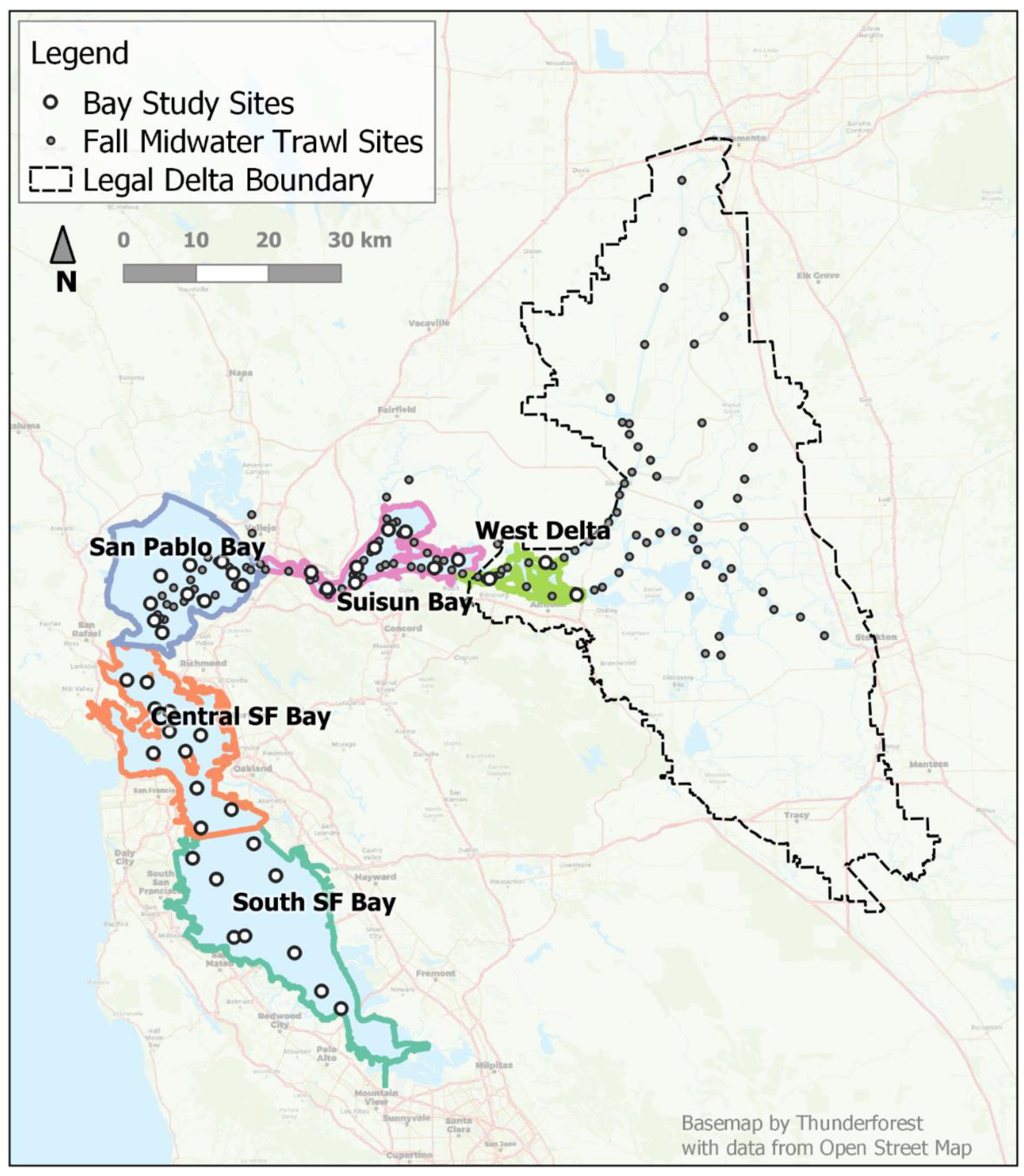
Figure 2.
An example of the range of wiggliness in smooth functions produced by generalized additive models (GAMs) with different maximum values for k. The smooth functions presented here represent the relationship between and the probability of catching a longfin smelt in San Pablo Bay and (left column) month of life and (right column) year class identified by birth year, shared across gear types, with various values of k. Lower values of k limit the number of degrees of freedom used to fit the curves.
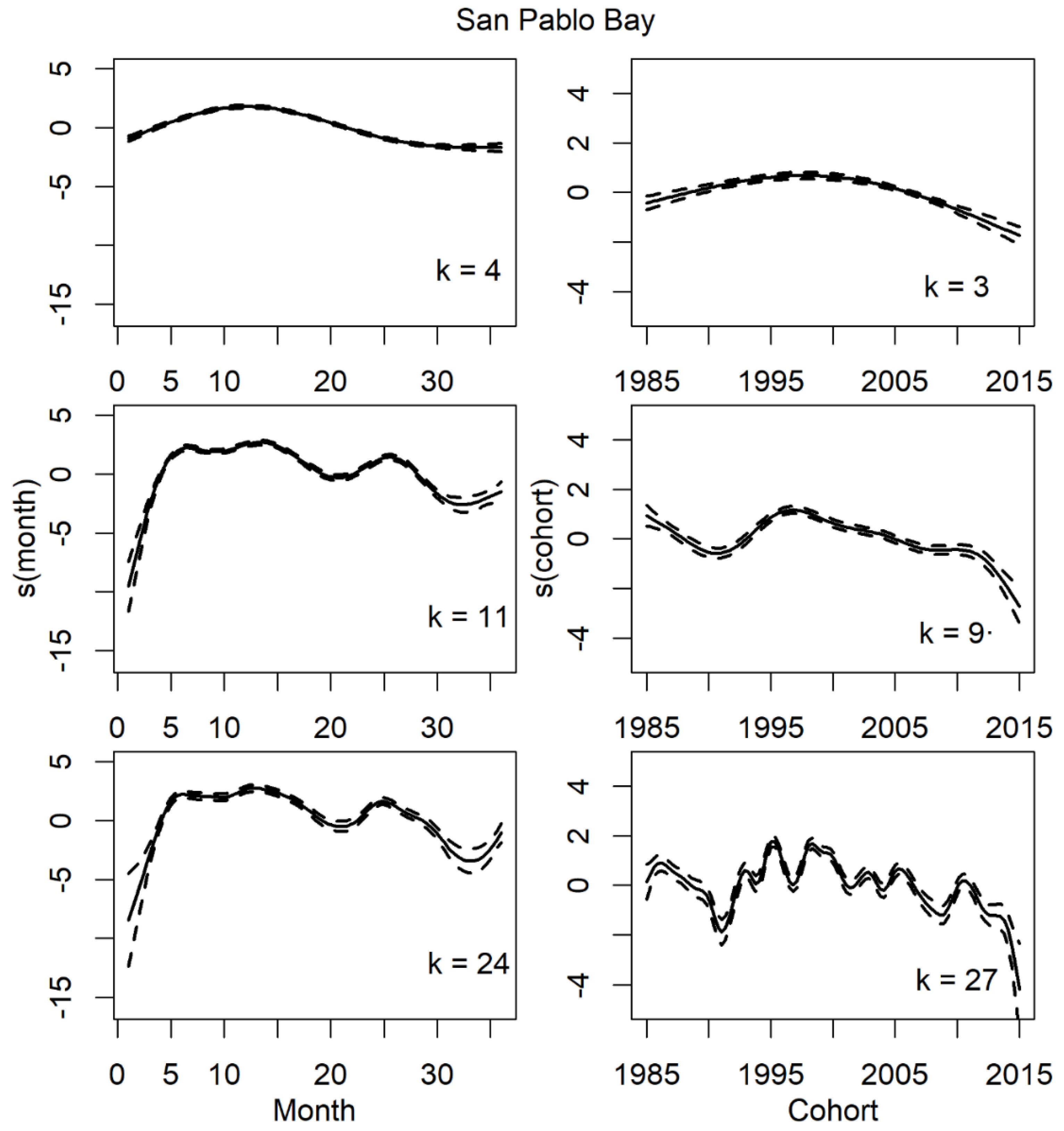
Figure 3.
Mean predicted probability of presence for each region by gear type and by month through the longfin smelt life cycle. These are functional means for each region, after registration of individual functions for each cohort that were obtained by generalized additive modeling (GAM).
Figure 3.
Mean predicted probability of presence for each region by gear type and by month through the longfin smelt life cycle. These are functional means for each region, after registration of individual functions for each cohort that were obtained by generalized additive modeling (GAM).
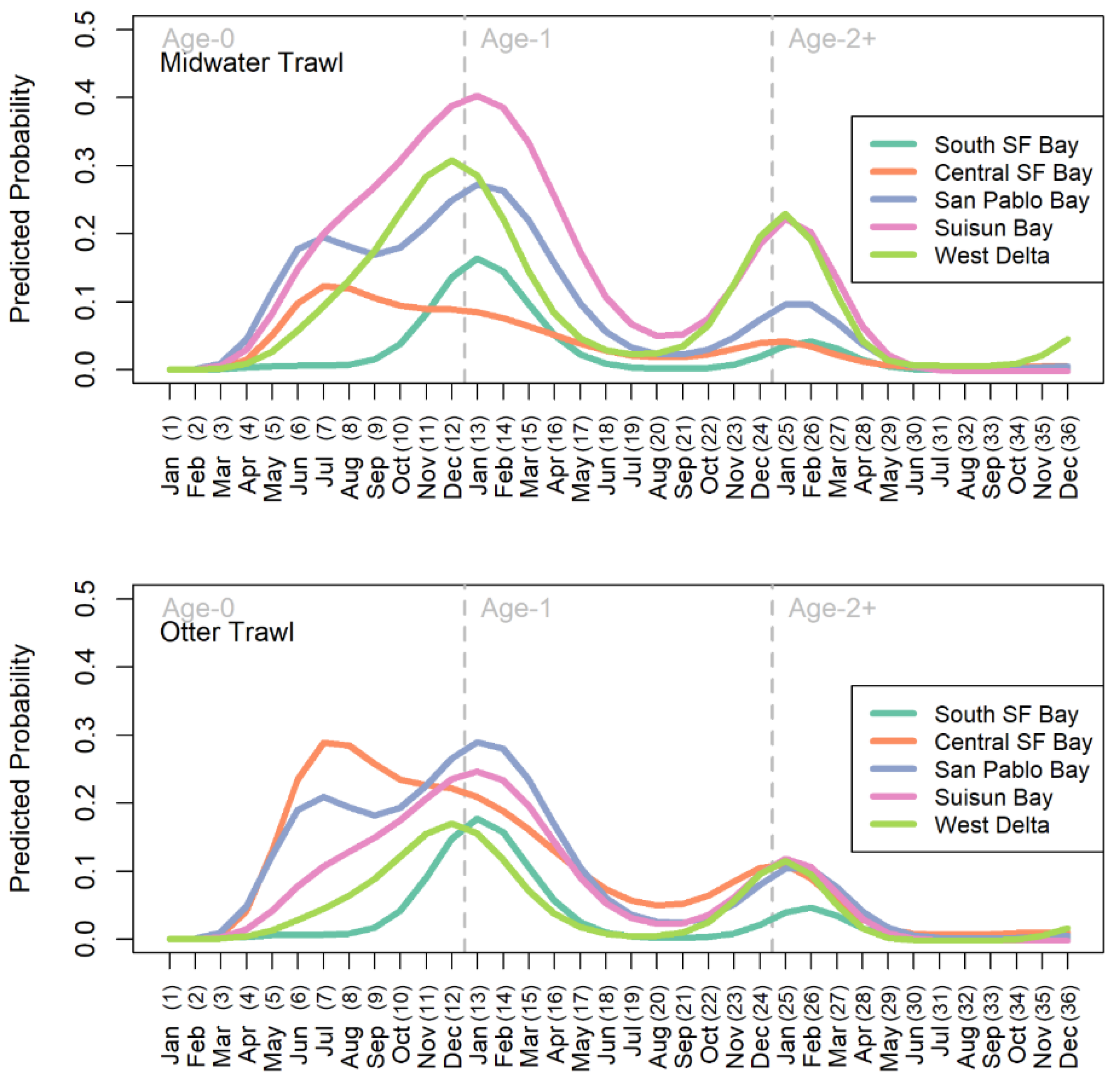
Figure 4.
The Fall Midwater Trawl total annual abundance index (top panel) and constituent monthly indices for longfin smelt over time. Water year types are categories that represent a range of hydrologic states from driest to wettest: critical (C), dry (D), below normal (BN), above normal (AN), and wet (W).
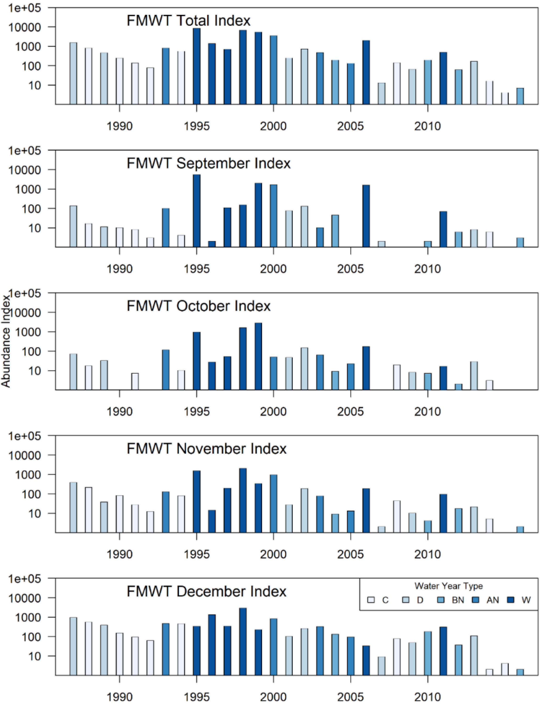
Figure 5.
Graphs illustrating the results of aligning functions representing model-predicted probabilities of catching longfin smelt using the San Francisco Bay Study’s midwater trawl gear (left column) in each region of the Estuary (rows) over their life span by separating the amplitude (middle column) and phase (right column) variation components of the annual probability functions. In the warping function graphs, warping distance values above zero indicate that the timing of a pattern has shifted later and values below zero indicate that the timing has shifted earlier.
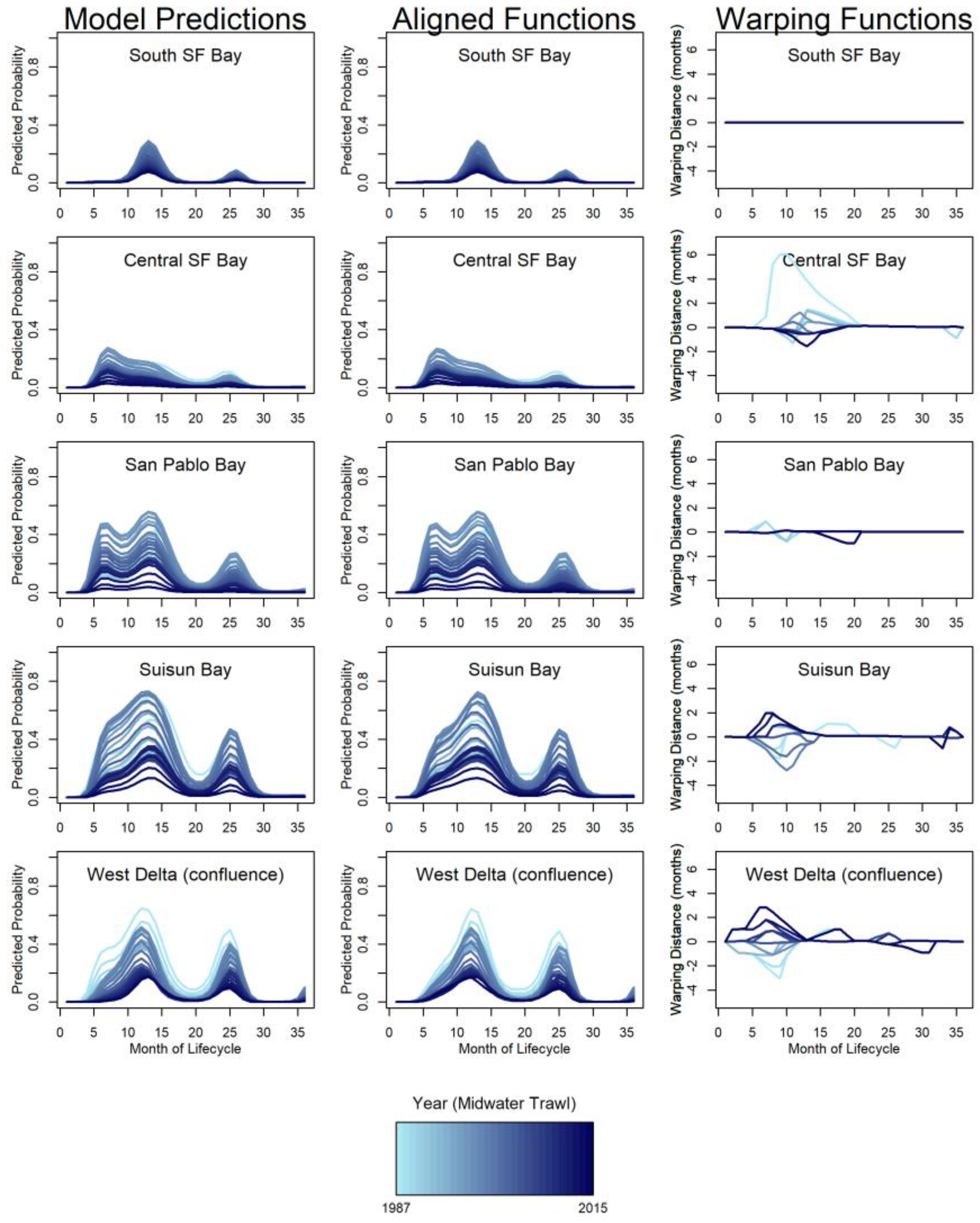
Figure 6.
Graphs illustrating the results of aligning functions representing model-predicted probabilities of catching longfin smelt using the San Francisco Bay Study’s otter trawl gear (left column) in each region of the Estuary (rows) over their life span by separating the amplitude (middle column) and phase (right column) variation components of the annual probability functions. In the warping function graphs, warping distance values above zero indicate that the timing of a pattern has shifted later and values below zero indicate that the timing has shifted earlier.
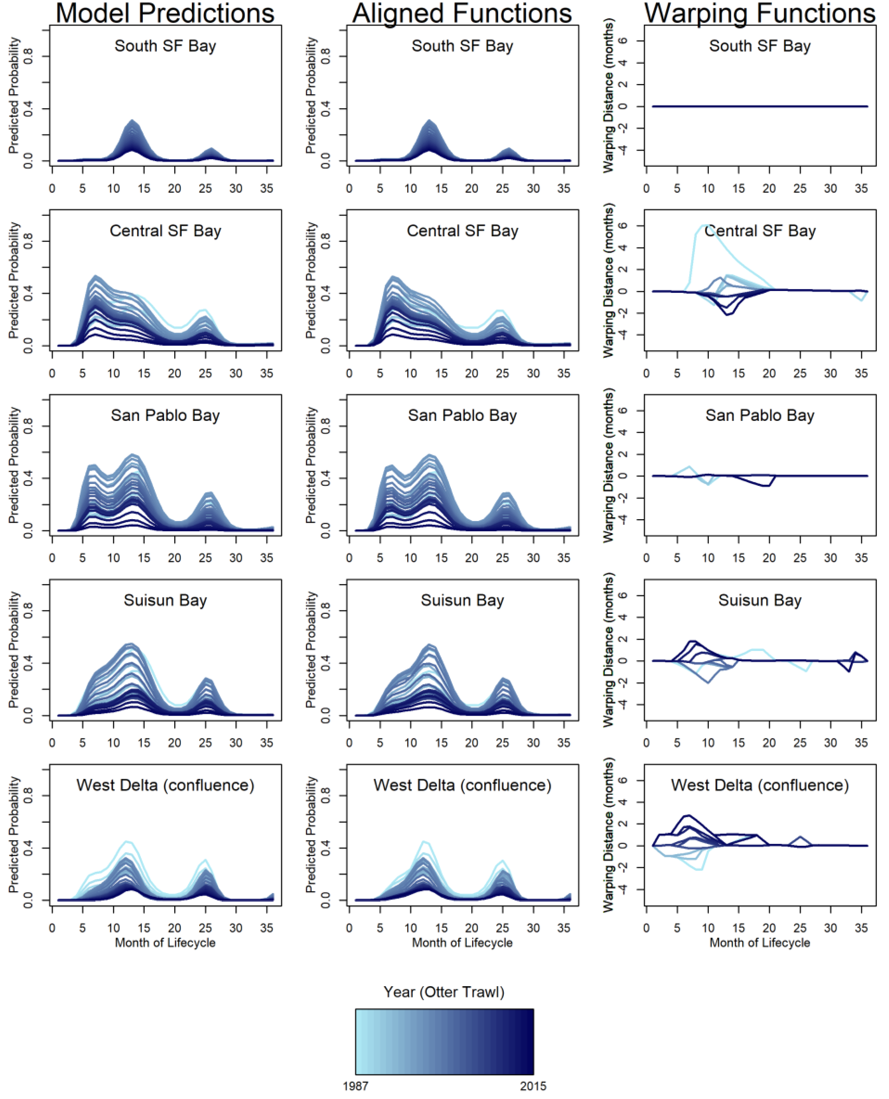
Figure 7.
Shifts in timing of longfin smelt presence in the three regions of the San Francisco Estuary. Lines represent trends for whichever month had the highest phase variability for each of the regions with spikes in phase variation, as indicated in the legend. South SF Bay and San Pablo Bay did not have spikes in phase variation so those were not included. The horizontal dashed black line at 0 indicates the mean timing of longfin smelt presence for each region.
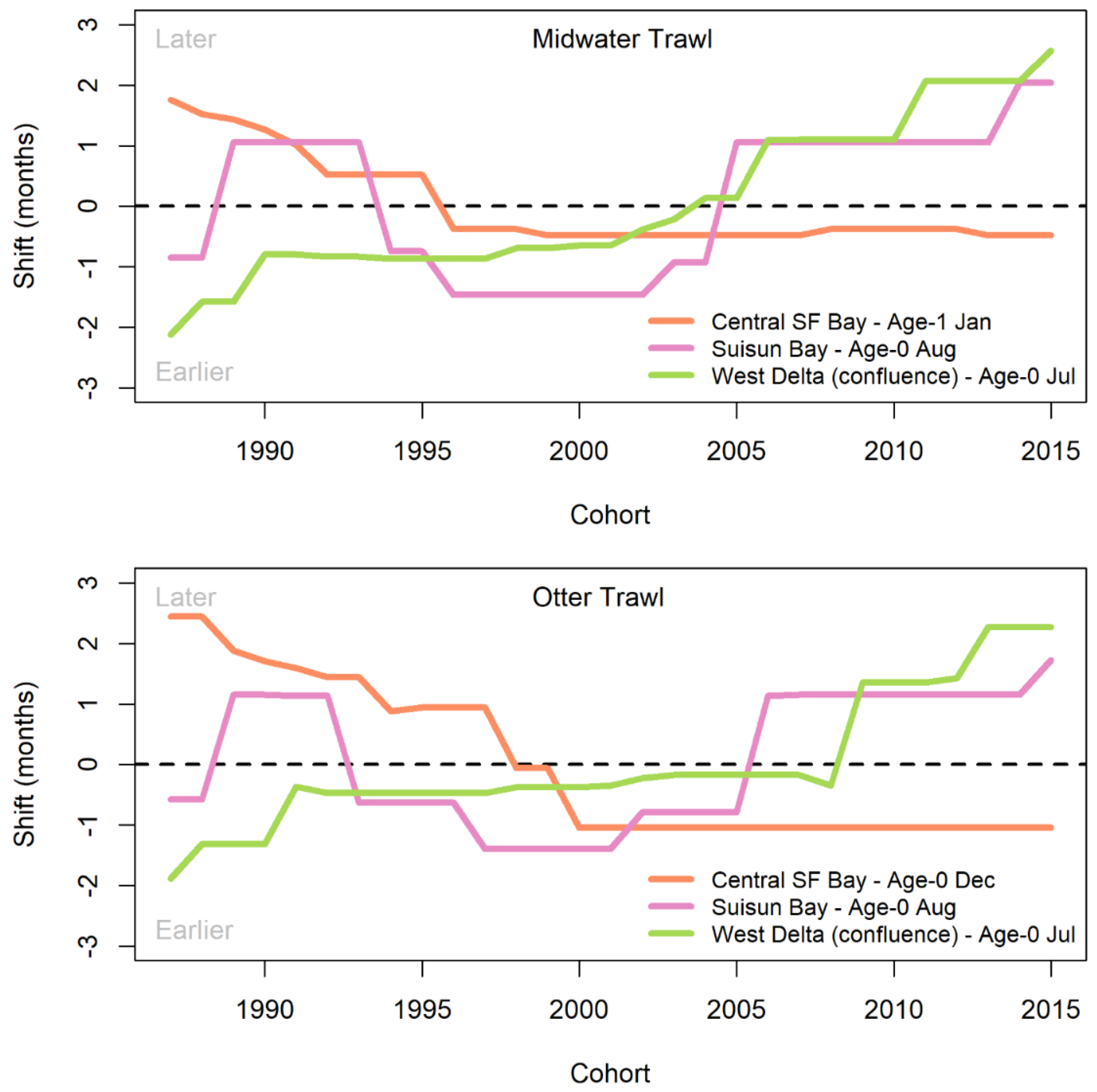

Table 1.
Criteria for assigning age based on length. Fish that were larger than the age-1 maximum criteria for a given month were assigned to the age-2 group.
Table 1.
Criteria for assigning age based on length. Fish that were larger than the age-1 maximum criteria for a given month were assigned to the age-2 group.
| Month | Age-0 Maximum Length (mm) | Age-1 Maximum Length (mm) |
| January | 40 | 90 |
| February | 42 | 93 |
| March | 46 | 96 |
| April | 52 | 100 |
| May | 59 | 105 |
| June | 67 | 108 |
| July | 71 | 111 |
| August | 75 | 114 |
| September | 80 | 117 |
| October | 83 | 120 |
| November | 85 | 122 |
| December | 87 | 124 |
Table 2.
Estimates for parametric coefficients and smooth terms for the selected model. The baseline conditions for parametric coefficients (i.e., where the categorical variables are equal to zero) are bay1 and midwater trawl. Parametric estimates and standard errors are presented in logit-scale. Bay/Region numbering is as follows: 1 = South SF Bay, 2 = Central SF Bay, 3 = San Pablo Bay, 4 = Suisun Bay, 5 = West Delta.
| Parametric Coefficients: | ||||||||
| Term | Estimate | Std. error | z value | Pr(>|z|) | ||||
| (Intercept) | -5.18 | 0.18 | -28.37 | < 2e-16 | ||||
| gear:otter trawl | 0.10 | 0.10 | 1.04 | 0.30 | ||||
| bay2 | 0.76 | 0.21 | 3.60 | 0.00 | ||||
| bay3 | 1.66 | 0.20 | 8.20 | 0.00 | ||||
| bay4 | 2.26 | 0.21 | 10.91 | < 2e-16 | ||||
| bay5 | 1.25 | 0.30 | 4.14 | 0.00 | ||||
| otter trawl:bay2 | 1.01 | 0.12 | 8.68 | < 2e-16 | ||||
| otter trawl:bay3 | -0.01 | 0.11 | -0.09 | 0.92 | ||||
| otter trawl:bay4 | -0.90 | 0.11 | -7.95 | 0.00 | ||||
| otter trawl:bay5 | -0.90 | 0.15 | -5.90 | 0.00 | ||||
| Approximate significance of smooth terms: | ||||||||
| Term | edf | Ref.df | Chi.sq | p-value | k' | edf | k-index | p-value |
| s(month):bay1 | 9.28 | 9.83 | 579.57 | < 2e-16 | 10 | 9.28 | 0.97 | 0.57 |
| s(month36):bay2 | 9.74 | 9.97 | 872.40 | < 2e-16 | 10 | 9.73 | 0.97 | 0.49 |
| s(month):bay3 | 9.80 | 9.99 | 1030.57 | < 2e-16 | 10 | 9.80 | 0.97 | 0.52 |
| s(month):bay4 | 9.71 | 9.97 | 1086.78 | < 2e-16 | 10 | 9.71 | 0.97 | 0.50 |
| s(month):bay5 | 9.29 | 9.82 | 269.28 | < 2e-16 | 10 | 9.29 | 0.97 | 0.45 |
| s(cohort):bay1 | 5.20 | 6.22 | 51.64 | 0.00 | 8 | 5.20 | 0.98 | 0.74 |
| s(cohort):bay2 | 7.56 | 7.93 | 202.43 | < 2e-16 | 8 | 7.56 | 0.98 | 0.74 |
| s(cohort):bay3 | 7.71 | 7.97 | 325.31 | < 2e-16 | 8 | 7.71 | 0.98 | 0.74 |
| s(cohort):bay4 | 7.70 | 7.97 | 393.79 | < 2e-16 | 8 | 7.70 | 0.98 | 0.70 |
| s(cohort):bay5 | 5.88 | 6.87 | 76.39 | 0.00 | 8 | 5.88 | 0.98 | 0.75 |
| ti(month,cohort):bay1 | 1.96 | 2.44 | 1.42 | 0.61 | 16 | 1.96 | 0.94 | 0.01 |
| ti(month,cohort):bay2 | 6.47 | 8.65 | 38.30 | 0.00 | 16 | 6.47 | 0.94 | 0.03 |
| ti(month,cohort):bay3 | 7.73 | 10.10 | 33.24 | 0.00 | 16 | 7.73 | 0.94 | 0.02 |
| ti(month,cohort):bay4 | 10.55 | 12.67 | 42.48 | 0.00 | 16 | 10.55 | 0.94 | 0.03 |
| ti(month,cohort):bay5 | 8.14 | 10.31 | 20.05 | 0.06 | 16 | 8.14 | 0.93 | <2e-16 |
Table 3.
Variance in functions representing predicted probabilities for each bay/region and gear type. Each variance value was derived from the registration of 28 predicted probability curves. Values given with 3 significant figures. Variance in amplitude is relative to the probability of observing longfin smelt; units for phase variance are months.
| Region Number | Region Name | Midwater Trawl | Otter Trawl | ||
| Amplitude | Phase | Amplitude | Phase | ||
| 1 | South SF Bay | 0.0141 | 0.00 | 0.0163 | 0.00 |
| 2 | Central SF Bay | 0.0264 | 0.000184 | 0.108 | 0.00167 |
| 3 | San Pablo Bay | 0.18 | 0.000986 | 0.198 | 0.00113 |
| 4 | Suisun Bay | 0.296 | 0.0106 | 0.163 | 0.00321 |
| 5 | West Delta | 0.113 | 0.0129 | 0.0517 | 0.00262 |
Disclaimer/Publisher’s Note: The statements, opinions and data contained in all publications are solely those of the individual author(s) and contributor(s) and not of MDPI and/or the editor(s). MDPI and/or the editor(s) disclaim responsibility for any injury to people or property resulting from any ideas, methods, instructions or products referred to in the content. |
© 2025 by the authors. Licensee MDPI, Basel, Switzerland. This article is an open access article distributed under the terms and conditions of the Creative Commons Attribution (CC BY) license (http://creativecommons.org/licenses/by/4.0/).
Copyright: This open access article is published under a Creative Commons CC BY 4.0 license, which permit the free download, distribution, and reuse, provided that the author and preprint are cited in any reuse.


