Submitted:
02 February 2023
Posted:
02 February 2023
Read the latest preprint version here
Abstract
This study describes all the properties of high Tc cuprates by introducing rotating holes that are created by angular momentum conservations on a 2D CuO2 surface, and which have a different mass from that of a normal hole because of the magnetic field energy induced by the rotation. This new particle called a macroscopic Boson describes the doping dependences of pseudo-gap temperature and the transition temperature at which an anomaly metal phase appears and describes the origin of the pseudo-gap. Furthermore, this study introduces a new model to handle many-body interactions, which results in a new statistic equation. This statistic equation describing many-body interactions accurately explains why high Tc cuprates have significantly high critical temperatures. Moreover a partition function of macroscopic Bosons describes all the properties of anomaly metal phase, which sufficiently agree with experiments, using the result from our previous study [1] that analytically describes the doping dependence of Tc. By introducing a macroscopic Boson and the new statistical model for many-body interactions, this study uncovered the mystery of high Tc cuprates, which have been a challenge for many researchers. An important point is that, in this study, pure analytical calculations are consistently conducted, which agree with experimental data well (i.e., they do not use numerical calculations or fitting methods but use many actual physical constants).
Keywords:
high Tc cuprates
; macroscopic Boson
; many-body interactions
; pseudo gap
; critical temperature
; anomaly metal phase
; conservation of angular momentum
; attractive force
; Cooper pair
1. Introduction
First of all, note that, as the abstract mentioned, the present paper is written under the condition that our previously published article [1] was understood that describes the Tc formula analytically, although the present paper will provide the review sections.
Although several significant advancements have been presented, from the initial discovery of a superconductor, the most impressive discoveries are CuO2-based superconductors (i.e., high-Tc cuprates) [2].
This is because, prior to this result, superconductors generally require significantly high refrigeration because of their lower critical temperature (~20 K). However, because they have higher Tc than LN2, the high-Tc cuprates received considerable attention and interests from condensed matter physics researchers and researchers in technologies who demonstrated interest in the technical merits when applied to superconducting magnetic energy storage and energy transmission [3–5].
Thus, initial results demonstrated that high-Tc cuprates involved researchers from many condensed matter physics and related technologies.
However, condensed matter physics researchers investigated high-Tc cuprates for much deeper reasons, i.e., they are the first case at which the standard band model and the Bardeen–Cooper–Schieffer (BCS) theory are not applied, which indicates that novel physical phenomena occurred. (Recent H-based superconductors [6] with extremely high pressures have high potential to be applied to the BCS theory.) Moreover, many claimed that it is related to many-body interactions [7], which made many theoretical researchers’ approaches to the mechanism difficult. It is obvious that, similar to the BCS theory, the use of quantum field theory is not adequate because quantum field theory is extremely abstract and does not reflect the fact that a phenomenon in condensed matter physics involves many actual physical constants.
Although many studies about the experiments have been reported [8–13], (in particular, STM and STS [15] experimental methods to date revealed many aspects in high-Tc cuprates,), no theory describes all of the experimental data. These theories are divided to two methods: either Fermi-liquid model or resonating valence bond (RVB) model [16–19].
However, these theories have undetermined parameters, which inevitably leads to numerical or fitting methods. We must mention that they are insufficient because many related and actual physical parameters (i.e. physical constants) are involved when the properties of high-Tc cuprates are considered. For example, several researchers claim that, because of the existence of magnetic-field interactions, the natural force to combine a Cooper pair must be spin interactions. However, as mentioned in this study and our previous study [1], magnetic-field interactions are not generally only the spin interactions. For example, the spin-fluctuation [19] model is a numerical one; in this sense, this model is similar to the Hubbard-like model [20]. These models have multiple parameters to determine or to fit; thus, they do not reflect actual physical picture the high-Tc cuprates originally have.
Furthermore, if the interaction was defined as spin interactions, they could not explain why other multiple physical parameters such as phonons are related [21].
Although multiple theories exist discussing the nature of force to combine a Cooper pair and the origin of pseudo-gap using RVB model or Hubbard-like model, few theoretical articles analytically address and explain experiments data, in addition to the anomaly metal phase and the transition temperature T0 at which the anomaly metal phase appears.
Briefly, the understanding of high-Tc cuprates requires
- Analytical calculations of many-body interactions. Most theories use a numerical or fitting method; however, these approaches cannot clarify the physical picture in high-Tc cuprates.
- To understand the nature of force to combine a Cooper pair over long distance.
However, research-related challenges have prevented a complete investigation of the abovementioned issues. If the calculations can be analytically solved, condensed matter physics will make considerable progress in developing then methods for fabricating compounds with higher critical temperatures could be developed through condensed matter fields. Thus, uncovering the physical mechanics of high-Tc cuprates is urgently required, and has motivated the present study. We thus provide new answers to the above questions.
Combining with our previous study [1], we will propose a concept of macroscopic Boson. This paper will describe the mechanism of high-Tc cuprates, using only this concept, with the consideration of many-body interactions.
As the contents of this paper, first we introduce a concept of macroscopic Boson, in which its mass and spin are described. Then using the partition function, the pseudo-gap energy is explained. Moreover, the method to handle many-body interaction will be introduced. Next, as the review, we obtain the formula of Tc [1]. The calculations of obtaining formulas of T* and T0 are positioned, analyzing anomaly metal phases. Section 3 is Method in which more concrete calculation methods are indicated. Then Result and Discussion sections are followed. Finally, the paper concludes the entire contents in section 6.
2. Theory
2.1. Introduction of new particle and pseudo-gap relating to new particle
2.1.1. Introduction of a macroscopic Boson
When considering a CuO2 surface as the most important point [22] and when the refrigeration is sufficient such that a hole’s wavelength becomes larger than that of width of the surface, it is assumed that 2D is completely formed. This indicates that, on the surface, an angular momentum must be conserved; thus, each hole takes a circle by self-rotating. At this time, because this rotating circle has magnetic field energy, we consider that a new particle has been created. Note that the creations of the particles implies a phase transition, which will be described later in this paper. This is related to the electron nematic phase [27]. Going forward, we refer to this new particle as a “macroscopic Boson”; the schematic is shown in Figure 1.
2.1.2. Calculating the mass of a macroscopic Boson
First, let us calculate the mass of a macroscopic Boson. Using a magnetic flux, magnetic field energy is represented as follows:
where I and Φ0 denote a current surrounding a macroscopic Boson and a magnetic flux of a macroscopic Boson having a unique value. In this equation, the magnetic flux is assumed to be quantized because each angular momentum is conserved as mentioned.
where h and e denote the Planck constant and the charge of a hole, respectively. Note that this study used both the constant h and ħ as Planck constants. Note that this quantization implies that each flux behaves as a particle, as discussed.
In this current, the cyclotron angular frequency is introduced.
where ωc, B0, and u0 denote the cyclotron angular frequency, the constant and unique value of magnetic field in a macroscopic Boson, and the magnetic permeability in the vacuum, respectively. Thus, eq. (1) becomes
where considering a flux of eq. (2)
where η is the approximated radius of a macroscopic Boson.
Because the magnetic field B0 is expressed as eq. (5), the rest energy, i.e. the mass of a macroscopic Boson is formed as follows:
2.1.3. Spin of a macroscopic Boson
Let us now consider the spin of a macroscopic Boson to obtain partition function, which creates all the anomaly metal properties. As mentioned, when a macroscopic Boson is created, a complete 2D motion can be considered. That is, among the x-y-z axes, we cannot consider z-components; therefore, using the Pauli matrix, this case considers only the x- and y-components.
In this study, a spin angular momentum is defined as the determinant from the Pauli matrix.
Thus, each determinant is as follows:
Therefore, a net spin angular momentum of a macroscopic Boson is calculated as follows:
The above result indicates that, although a single hole behaves as a Fermion, this macroscopic Boson on 2 D behaves similar to a Boson. Thus, the name of this particle is derived from this fact.
Let us consider this by another view:
It is necessary to consider a magnetic-flux property in terms of the electromagnetics. As described, a macroscopic Boson is simply a magnetic flux in a 2D sheet. Moreover, electromagnetic energy is expressed by the following Hamiltonian [33];
While time-dependent energy is described by the first term in this equation, a static magnetic field energy, i.e., the energy of a macroscopic Boson, is equal to the second term, i.e., the zero-point energy [33]. On the other hand, the liquid He (i.e., quantum liquid) has also the zero-point energy [33]. Because the liquid He is consisted of Bose particles, a macroscopic Boson can be considered to be a boson.
As described, as long as considering 2D, the statistic property would alter.
2.1.4. Obtain the partition function
Because a macroscopic Boson on 2D follows the Bose’s partition function, we simply must consider the following:
where Ei, , ,and T denote energy, a chemical potential (i.e. ), the Boltzmann constant, and temperature, respectively. An important point is that the exponential function is approximated as a Maclaurin series,
This abovementioned partition function is very important because all properties in the anomaly metal phase in CuO2-based superconductors are described using this partition function. We will see how this equation describes properties of the anomaly metal phase later.
Moreover, this equation has another expression. Because we are now considering the chemical potential from Bosons and the general boson partition function, the following equation generally holds:
where the absolute value of the second term must be dominate over the value of the first term because the chemical potential is negative, and where denotes accepter concentration. Moreover, indicates a doping parameter in this study. The number 2 is attached because of the presence of spin. Therefore, because ni indicates the concentration of lattices, of ln is less than the value of the number 1 as long as we consider the image in which holes are doped in a Mott insulator.
Using the equation above, the partition function, eq. (11), is translated as follows:
2.1.5. Calculate the pseudo-gap energy
Let us calculate the pseudo-gap energy, which is directly related to the mass of a macroscopic Boson. First, we define the carrier concentration of macroscopic Bosons considering a 2D energy state density.
where , n, and d denote energy state density in 2D, particle concentration, and width of the 2D sheet, respectively. An important point to note is that the parameter d [m] is consistently substituted by the number 1; however, the reason of the appearances in certain equations clarify the meaning of these equations. The integral for concentration (14) is simply as follows because the energy state density in 2D is constant as indicated in eq. (13) and because partition function fr is represented by eq. (11-2). In the process of this calculation of eq. (14), an energy E0 appears as follows:
This energy E0 is assumed to be essentially equal to the pseudo-gap energy. Combined with the mass of a macroscopic Boson, this pseudo-gap energy is represented as follows:
The abovementioned pseudo-gap energy equation has a coefficient for doping function ln. This factor is identical to the zero-point energy:
The above equation implies that this derived energy E0 merely indicates a potential. In general, however, an energy gap appears or disappears involving a photon’s emission or absorption, which has a momentum. This fact indicates that, for a potential to become a general energy gap, the potential is given the product of the fine-structure constant α, which includes characteristic impedance Z0 for electromagnetic waves. Typically, the fine-structure constant α is determined as follows:
In eq. (17), the impedance Z0 works as the specific impedance to electromagnetic waves. Thus, the net pseudo-gap energy is derived as follows, which will give the temperature of pseudo-gap T* as discussed later.
2.2. Superconductivity with consideration of many-body interactions
It is necessary to describe why macroscopic Bosons undertake Bose–Einstein (BE) condensation by forming a pair from two macroscopic Bosons, although they have been already general Bosons such as Cooper pairs. In the previously published paper [1], we reported a new attractive force to combine particles from local current in a CuO2 cell [27]. This local current is equal to both rotational and self-current, which creates the mass of macroscopic Bosons; hence, the result of the previous paper agrees with the descriptions in the present paper. Therefore, in this section, based on the understanding that two macroscopic Bosons form a pair, we describe why BE condensation occurs considering many-body interactions between Bosons.
2.2.1. Description of the model and the principle to many-body interaction
There are many-body interactions among the carriers in various materials. In particular, this fact is essential to high-Tc cuprates because the general band theory cannot be applied. The many-body interactions of carriers indicate there are many local temperatures Ti in the materials, where i is index for a location. In other words, only in a temperature Ti, thermal equilibrium can be assumed. Figure 2 shows our model for handling many-body interactions. In this figure, a radius ai forms a sphere shell, which has differential number dN and local temperature Ti. Moreover, in the center, a macroscopic Boson is presented. The immediately outer particles out of dN yield a pressure to this sphere shell, which is equal to the kinetic energies of particles in dN (i.e., it is represented by a temperature Ti). However, the central macroscopic Boson provides force of expansion, which indicates electrostatic energy, i.e., Coulomb interactions. Moreover, this case adds magnetic interactions between macroscopic Bosons as an expansion force.
Considering that these forces of expansion should be balanced to a force of compression in a sphere shell, the following relation holds:
2.2.2. Calculate the principal equation of our model and the internal quantum state
Calculate the abovementioned principle equation. First, dN is represented as follows:
where k, v, g, and f denote wave number, volume, state number, and partition function for the Boson, respectively. In the equation of dN, as mentioned, state number g and partition function f are given as follows:
Thus, fg is given as follows:
To calculate the left-hand side of the abovementioned balanced equation in principle, the electrostatic energy UE is calculated as follows:
where and denote the permittivity for the vacuum and the radius which dN is taking in the model.
At this time, a volume element of the integral is expressed as follows:
Moreover, the magnetic interaction Vp from macroscopic Bosons is given as follows:
Consequently, the resultant equation is provided by
As shown in Figure 3, the central macroscopic Boson behaves under the model of the infinite well-potential. Thus, as every elementary quantum mechanics text [24] describes, the eigenvalue and wave function of it are presented as follows:
where M, i, and r denote the mass of a macroscopic Boson, index, and microscopic variable of sphere-coordinates, respectively. These equations indicate that a particle under the many-body interactions forms a stationary wave and that the wave function of the stationary wave and the eigenvalue (i.e., kinetic energy) are determined by a radius ai..
2.2.3. Describe BE condensation and the superconducting transition
Using the abovementioned concept, we consider how BE condensation occurs. In addition to a sphere shell having temperature Ti,, another sphere shell having temperature Tj is considered. When we accept a combination of two macroscopic Bosons by a force F, these two Bosons must have the identical kinetic energy because, in general and as mentioned in our previous paper [1], a relative and attractive force appears only when their relative velocities become the same. In particular, this fact is applied when an attractive Lorentz force is generated between moving and charged particles whose velocities are identical. Thus, when forming a pair from two macroscopic Bosons, the eigenvalues, eq. (26), indexed by i and j becomes equal. That is,
This indicates that an index i and j becomes equal, resulting in that all the radius ai and eigenvalue Ei take the identical radius a0 and EB because of the arbitrary property of index i and j. Hence, if a pair forms, every energy of macroscopic Bosons undergoes the identical energy EB, which indicates all the rest Bosons take pairs and BE condensation.
Moreover, as shown in Figure 4, considering index i to be equal j indicates that temperatures Ti and Tj must be equal. Even at this moment, positions r of wave functions, eq. (25), are common and thus the two sphere shells take the superposition, i.e. the relative distance ξG between the two sphere shells should be 0. Thus, the net coherence of two holes becomes on a cell order, 1 nm, as reported by many literatures.
Employing the abovementioned equation (24), an equation of the relative distance between sphere shells ξG for temperature T is derived as follows:
where UB is substituted with pseudo-gap in eq. (18). Note that, in this equation, considering BE condensation and single-particle picture, p0 of gf in eq. (20) is redefined as the value 1.
As will be discussed in the Results section, temperatures at which indicates a superconductivity state (i.e., the net coherence of two holes is about 1 nm, which equals CuO2 cell order) and the transition temperature Tc at which indicates a critical temperature.
2.3. Review to obtain the formula for Tc
Herein, we would like to note the reason why there are Fermi energy and chemical potential EF [25]. Considering each pair and because these pairs have superposition, a single macroscopic wave with a converged phase is produced. However, at this stage, although we cannot consider each particle motion as a pair of two macroscopic Bosons, there is a non-zero temperature (i.e., ). This indicates that the internal particles of a macroscopic Boson (i.e., holes) collide with each other. Thus, only in the case of , we consider the Fermi energy, i.e., .
2.3.1. Derivation of a general energy gap (review)
Let us review our previous study [1], which describes a force F to combine two particles and a critical temperature Tc on doping. Note that because this is a review to understand the stream of outlined derivations of a critical temperature Tc, certain equations in the calculation and derivation processes are left out. In case that our readers are interested in the detail, the paper can be downloaded as an Open Access paper.
First, we assume that a general energy gap is proportional to both Fermi energy and Critical temperature as follows [1]:
In this equation, the Fermi energy in a p-type material [40] is employed as follows:
Note that we are considering the carrier is a hole.
In this equation, a superconducting energy gap is introduced.
Substituting these energies and employing the state equation with the universal gas constant R, the following equations are obtained.
and
where
where denotes a thermodynamic potential, and ρs is the concentration of Cooper pairs.
In this manner, a general expression of energy gap for temperatures is derived.
2.3.2. Generation of an attractive force that combines two carriers (review)
To consider the superconducting energy gap, it is necessary to mention a force F, which results in a combination of a Cooper pair. As previously mentioned, two charged particles generally experience an attractive force with each other when they are moving with the same velocity, i.e., when the relative energy or momentum is 0. As shown in Figure 5a–5d, two parallel conductors along which the same direction and same amount of a current are presented. From the electromagnetism, these current leads experience an attractive force with each other, which is attributed to the Lorentz force. When we shorten these leads to a wavelength of a carrier, this attractive force still exists. This indicates that two charged particles with identical wave numbers are attracted to each other. This attractive force stems from the Lorentz force.
2.3.3. Derivation of Tc (review)
Considering the principle of generating an attractive force and assuming that the wave function of a hole is a plane wave and that the magnetic field generated by the moving holes is derived from a linear current, the Lorentz force F is given as follows:
where ψ, r, θ, ϕ, q, β, k m, and μ0 denote wave function of a hole, relative distance of two holes, angle associated with the Lorentz force, angle related with two wave number of holes, the electric charge of a hole, constant, common wave number, the mass of an electron, and magnetic permeability of the vacuum, respectively.
Note that this equation employs the probability density flux as current density.
The energy u (i.e., superconducting energy gap) from the line integral of the above force F is represented as follows:
where denotes an integral constant.
Furthermore, the derived superconducting energy gap u produces Tc with the combination of a general gap energy derived in eq. (33).
where
In this process, we added a Debye temperature θD and a net coherence ξ to the equation. Note that, as an integral constant in eq. (36), the BCS formula under a particular condition was employed. That is, in the formula Tc of the BCS theory, because the Boson combination energy in high-Tc cuprates is generally sufficiently large attributed to the short coherence (note that, the shorter the coherence is, the larger the magnetic field associated with the Lorentz force becomes), the large value of NV in the BCS formula of Tc makes the exponential function be almost the value 1. Thus, only the Debye temperature in the BCS formula is left. Concerning the thermodynamic potential, the following equation is applied under the condition of BE condensation.
where EF0 and EG0 denote the Fermi energy and band gap at zero temperature, respectively. Moreover, here the volume V is assumed to be the unit, i.e. the number 1. Thus, the critical temperature becomes
Moreover, we derive a 2D critical temperature equation from the above. Thus, to conclude, the critical temperature equation is derived as follows:
where σ, σs, θD2, and nq denote the surface density of carriers, the surface density of pairs, Debye temperature in 2D, and the number of layers. Note that all constants in the consequent equation have actual physical meaning and unit. This indicates that no numerical calculations or fitting methods are required. This fact is consistent everywhere in the present study.
Note that, in eq. (36) for the superconducting energy gap, the probability density function is interpreted as follows:
which shows that the gap is anisotropic [26]
In Figure 6, a result of this review section is shown where used physical parameters are listed in Table 1. Note that for additional details, please see the Method section at which the full list of employed physical constants are presented. As shown, our derived critical temperature equation sufficiently agrees with a typical high-Tc copulate. Note that the reason why the band gap is relatively large is related to the property of the Mott insulator. For more details, please refer to [1].
2.4. Calculations for obtaining formulas for T* and T0
2.4.1. Derive the pseudo-gap temperature T *.
Now, we consider the relation between a general energy gap and temperature, as shown in eq. (32)
When the previously derived energy gap from a macroscopic Boson is substituted for an energy gap in the abovementioned equation, then variable temperature T must become a constant of pseudo-gap temperature T*. Therefore, the temperatures Tc and T* have a dependent relationship. Thus, as a formula of pseudo-gap temperature T*, the following equation holds:
where to the equation of of eq. (18) in creating eq. (42), each physical parameter was substituted. That is, the physical parameters m, h, and α in eq. (18) were given actual values. Note that radius η is approximated as 1 nm.
2.4.2. Derive the transition temperature T0
In this study, we consider the anomaly metal phase properties in CuO2–based superconductors. These properties are primarily determined by the transition temperature T0, which is directly related to appearances of the Hall-effect coefficient RH. To obtain an equation for the temperature T0, we consider derivations of the Hall-effect coefficient RH. The Hall-effect coefficient RH depends on absolute of energy, –uBe,, where u and Be denote self-magnetic moment of a macroscopic Boson and applied magnetic field, respectively. The absolute of energy, uBe, involves Boltzmann statistics and thus it is related to concentration (i.e., the number) of macroscopic Bosons.
In the previously appeared concentration eq. (14), the calculation for energy integral, in turn, is actually conducted because we attempted to obtain temperature T dependence for RH
where
Note that the second form of fr in eq. (11-2) is not employed here. Eq. (43) is very important because the concentration n is proportional to the temperature T , which describes a property of the anomaly state. That is, the resistivity anomaly. Now we begin to calculate RH. As mentioned, considering an energy –uBe, the Boltzmann statics is represented as follows:
where n0 is concentration without an applied magnetic field. In this equation, the exponential function is approximated by the Maclaurin series.
In the above equation, the previously calculated concentration n, eq. (43), is applied.
Solving this equation for n0 and using the general definition of RH, we reach an important equation.
Composition of this equation presents a new temperature T0, which indicates the appearance of RH.
2.4.3. Implement the formulation of T0
To implement the formula T0, it is necessary to obtain u and Be in eq. (48). First, a magnetic moment u is generally defined as follows:
where I and S ( ) denote the self-current and the area in which a magnetic flux is presented. Seeing the schematic of Figure 1 of a macroscopic Boson (which assumes the motion of a hole to be a circle) and because a magnetic flux of it should be quantized as h/e, the magnetic flux of a macroscopic Boson is as follows:
That is,
(50-2)
where radius η is approximated on a cell of the CuO2 surface. That is,
Moreover, assuming that a magnetic field among a macroscopic Boson is equal to the central magnetic field generated by a moving hole, a persistent current I in a magnetic moment is calculated as follows:
Consequently, a magnetic moment u is derived as follows:
While an applied magnetic field Be in the definition of T0 is variable, the magnetic field B0 is a constant derived by the physical constants. This fact allows us to introduce a variable quantum number N between Be and B0
Moreover, this variable integer N is undergone by the partition function fr.
where eq. (11-2) is applied as fr.
Note that the magnetic field B0 was calculated from eq. (50-2). The employment of partition function fr indicates that an application of Be makes every direction of certain magnetic moments of macroscopic Bosons have the same orientation. In other words, prior to the application of magnetic field Be, the directions of self-magnetic moments of each macroscopic Boson are random (i.e., up- or down-direction), although the conservations of angular momentum produces macroscopic Bosons. However, the application of magnetic field Be presents all the directions of certain magnetic moments of macroscopic Bosons with the same orientation. Because the interaction between macroscopic Bosons with the same directed magnetic moment is repulsive, these Bosons now obtain the existences as single and independent particles. However, without an external applied magnetic field, why do our high-Tc cuprates become superconductive by forming many independent macroscopic Bosons? This can be understood by considering an analogy that every magnetic moment in a ferromagnetic material spontaneously acquires the same orientation under Curie temperatures. Thus, high-Tc cuprates have a property that is similar to a ferromagnetic material. We claim that this fact is related to the electronic nematic phase [27].
In this case, because macroscopic Bosons are formed in 2D CuO2, weak interactions between the magnetic moments of macroscopic Bosons can justify the abovementioned calculation. The actual calculations of Curie temperatures with complete consideration of many-body interactions are presented in the Appendix of this study.
Assembling these facts, the conclusive equation of the transition temperature T0 is derived, which depends on carrier doping.
As described later, this equation of T0 and the formula of critical temperature Tc [1] will be crucial factors when calculating properties of the anomaly metal phase.
2.5. Analyze anomaly metal phase
2.5.1. More comprehensive calculation of RH
Next, we derive dependences on temperature of RH. Up to the previous section, the general equation of RH was derived, which resulted in a definition of transition temperature T0. In this equation, we introduce the following approximation to the general equation of RH.
According to this approximation, the general equation of RH becomes as follows:
Thus, the approximated equation of RH is determined by the applied magnetic fields Be. That is, this RH equation depends on both quantum number N and the universal magnetic field B0.
Note that the universal magnetic field B0 is one in a macroscopic Boson. Thus, in view of magnetic field energy, an application of magnetic field, which dominates over the universal magnetic field B0 results in the destructions of macroscopic Bosons and makes the anomaly metal phase disappear. Moreover, the employment of quantum number N indicates that the RH equation is determined by doping. That is, variable integer N is expressed by the partition function fr, which indicates doping.
Considering this, the approximated RH equation becomes
As reported in many studies [28], this derived equation of RH is proportional to .
In the Results section, we will depict this RH equation in terms of both doping parameters and temperatures T.
2.5.2. Calculate the electron specific heat coefficient in the anomaly metal phase
In turn, let us consider electron specific heat coefficient in the anomaly metal phase. Because electron specific heat coefficient is essentially equal to the average energy UE, it is simply necessary to calculate the average energy using the partition function fr. Thus, average energy using partition function fr (eq. (11)) for energy integrals is determined as follows:
Note that the lower limitation a and the upper limitation b of these integrals are given as follows:
Assuming the chemical energy for macroscopic Bosons (i.e., not Fermi energy for single holes) is sufficiently small, the calculation results in
In general, electron specific heat coefficient is derived by differential in terms of temperature to the average energy. In this study, however, ΔT is employed rather than the differential for temperature. Moreover, this ΔT is assumed to be (T0-Tc) in this study. Therefore, using the average energy UE and ΔT, electron specific heat coefficient is expressed as a calculation process.
Furthermore, to obtain electron specific heat coefficient with the unit [J/mol K2], the Avogadro constant is considered because previously calculated average energy UE indicates one for a macroscopic Boson. Consequently, the electron specific heat coefficient is derived as follows:
2.5. Summary of the logical flow
- (1)
- First, assuming a macroscopic Boson, which is based on angular momentum conservation on a CuO2 surface, its energy was calculated; the implementation of the integral of the concentration resulted in a pseudo-gap energy. During this process, the two types of partition equations fr were derived.
- (2)
- To handle many-body interactions, a sphere shell with a local temperature Ti and differential particle number dN is introduced. From the forces that are balanced for both inside and outside the shell, a basic statistic equation, inner wave function and eigenvalue in a shell were derived.
- (3)
- The generation principle of attractive force: “The Lorentz force is applied between two charged particles when their relative velocity is 0.” Considering this principle, the abovementioned statistic equation, inner wave function and inner eigenvalue realize the combination of a Cooper pair, and then BE condensation occurs.
- (4)
- Therefore, the superconducting energy gap and Tc were calculated. During this process, a general energy gap is derived.
- (5)
- Combining the general energy gap and the mass of a macroscopic Boson, the pseudo-gap temperature, T*, formula was obtained.
- (6)
- The transition temperature T0 at which anomaly metal phase appears was defined by the appearance of the Hall coefficient RH. Thus, to calculate RH, combining the Boltzmann statistics, particle concentration was implemented using the partition equation fr. Then, the general definition of RH and the concentration produced the equation of RH. Considering the form of this equation, the transition temperature T0 was derived.
- (7)
- Because the resulted T0 has the magnetic moment of a macroscopic Boson u and magnetic field Be, these two factors were formulated. Thus, the T0 formula was implemented.
- (8)
- The abovementioned derived RH equation was approximated, and electron specific heat coefficient γ was calculated. Of note, during this process, the average energy using partition equations fr was obtained.
3. Methods
Herein, we describe the detailed method for the Results section.
3.1. Calculation tool
We employed the MS Excel software.
3.2. Physical constants for calculations
Table 2 shows the primary physical constant in this study. Of note, although Debye temperatures for 3D and 2D are different, we employed 2D one
3.3. Resulted equations
3.3.1. Critical temperature
The critical temperature is shown above again. Concerning anisotropic properties, sine and cosine are given the maximum values of 1. Table 2 lists the physical constant used except for concentrations.
3.3.2. How to determine ni and ρs
In eq. (40), is identical for , because the length along the c-axis, d, is consistently given the value of 1 by considering the 2D surface. Moreover, it is necessary to determine the values of 1/σs, i.e., 1/ρs when given the doping variable as follows:
(How to determine ni)
In this study, the concentration ni indicates lattice concentration. Because the unit cell of the CuO2 surface is of the 1-nm order, the following assumption is introduced
Note that d has the unit of [m] and the consistent value of 1 because we are considering two dimensions.
Because the critical temperature equation (40) uses the universal gas constant,
the concentration ni must be transformed into one with the unit [mol/L].
Thus, consider the following:
- 1)
- Avogadro constant
- 2)
- 1[L] =
Therefore the concentration ni is typically
(How to determine 1/ρs)
First, in the MS Excel sheet, the variable-doping ratio is in the range of 0.005–0.5. Note that the number 2 appears due to spins. Then, is calculated based on the abovementioned variable doping ratio.
1/ρs should be determined by the constant concentration, eq. (69)
where x denotes dimensionless variable. To give eq. (70-1) the meaning, variable x is provided as
3.3.3. Pseudo-gap temperature and transition temperature at which an anomaly metal phase occurs
We list the results of each transition temperatures, which will be shown in the Results section.
Of note, .
3.3.4. Physical results of the anomalous metal phase
(Hall effect coefficient)
Of note, . Because B0 is constant, the variation of integer N0 indicates variation in the applied magnetic field Be.
Moreover, in the abovementioned resulting equation, the following constants were employed.
(Electron specific heat coefficient)
3.3.5. Results of the many-body interaction model
where
Of note, in eq. (20), considering the BE condensation and single-particle picture,
The doping variable is fixed as a constant only in the abovementioned equation.
Note that, precisely, when , it should be considered that the doping is the cross point of Tc-dome and T*.
4. Results
First, Figure 7 shows the entire depictions of Tc, T*, and To on doping because of analytical calculations. Generally, the agreements with the experiments are good. Moreover, in Figure 8, the result of theoretical calculations of the Hall coefficient RH. As shown, the lower doping, the higher RH, and the RH behave as non-linear on temperatures.
Because of the statistic equation for the many-body interactions, Figure 10 shows superconductivity state up to a critical temperature ~140 K. In this figure, the state that relative distance between two spherical shells (i.e. two macroscopic Bosons) considering the many-body interactions is under 0 indicates the superconductivity state. From the further temperatures higher than the critical temperature, the relative distance becomes much larger as a change of non-continuity. Obviously, a transition occurs at ~140 K. This result accurately agrees with the experiments such as [28]. Furthermore, Figure 9 shows a result of theoretical calculation for the electron specific heat coefficient. According to the experiments [29,30], the calculation values are valid; moreover, it takes a maximum at a higher doping.
Importantly, in Figure 10, the magnetic field interaction UB in our statistic equation is substituted by the pseudo-gap energy at optimum doping. Thus, as many studies claim, the many-body interactions in terms of macroscopic Bosons are some of the reasons why high-Tc cuprates exhibit a considerably higher critical temperate. Moreover, for the determination of Tc, the pseudo-gap energy that is derived from the mass of a macroscopic Boson is crucial.
5. Discussion
5.1. Macroscopic Boson and high-Tc cuprates
We propose a particle describing high-Tc cuprates is not a normal hole but a macroscopic Boson, which is formed by the conservation of angular momentum in 2D and by rotational motion of a hole itself. The concept of a macroscopic Boson, as mentioned, provided a unique partition function; this partition function can explain every property in the anomaly metal phase. Moreover, the presence of this Boson gives substantial reason why high-Tc cuprates have significantly high critical temperature when considered with many-body interactions.
5.2. Anomaly metal phase and transition temperature T0
Thus far, to understand the mechanism of a high-Tc cuprate, it was important to study the source of pseudo-gap energy. Although this is true, another important factor that should be understood is the source of the transition temperature T0, which defines the anomaly metal phase appearance. As mentioned, all equations that describe the anomaly metal phase have the parameter T0 and Tc. Therefore, the excessive focus on the origin of pseudo-gap energy made most researchers less careful of the source of the transition temperature T0, and this attitude confused researchers when considering the mechanism.
5.3. Highlights of the process for the materials to undergo superconductivity
Let us review the process, which describes the mechanism from forming a macroscopic Bosons to undergoing BE condensation. First, high-Tc cuprate reaches the transition temperature T0 with a lower or no refrigeration. At this stage, because the wavelength of a hole along c-axis becomes longer than the width of a 2D CuO2 surface, the net 3D disappears and the conservation of angular momentum forms a macroscopic Boson, which indicates the rotation of a hole producing a magnetic field energy. Thus, this magnetic field energy gives a mass of macroscopic Boson.
By further refrigeration, our established statistic equation results in the following:
1. Many-body interactions, including the magnetic field energy of macroscopic Bosons and Coulomb interactions, result in very short relative distance of two holes (i.e., the net coherence of ~1 nm) as a result of all the sphere shells being superposed. Note that, at this stage, the paring of two macroscopic Bosons indicates the pairing of two holes.
2. Simultaneously, two holes gain a strong combination of the Lorentz force because the relative kinetic energy among two holes becomes 0; note that all Cooper pairs take the identical energy and thus BE condensation is produced, which is the source of the Meissner effect.
Although the derivation of a macroscopic wave function inevitably results in the London equation using the GL equation [31]; herein, let us review the reason why the Meissner effect is derived by another approach, thus stressing the converged and constant phase .
Under an applied magnetic field B (i.e., vector potential A), we can derive the Aharonov–Bohm (AB) effect [32] from the initial macroscopic wave function.
where q, j, and denote the hole charge, imaginary unit and converged phase of the macroscopic wave function, respectively.
From eq. (71), it is derived that
where n is the integer. Assuming n = 0, we have
and considering center-of-mass motion,
Substituting eq. (74) in eq. (73) and differentiating both sides of eq. (73), we obtain
The probability density flow is then defined as follows:
Substituting eq. (75) in eq. (76-1), we derive the following London equation:
This is the identical result from approaches by the GL equation [36].
5.4. The reason why high-Tc cuprates have significantly high critical temperature
As mentioned, an attractive force is the Lorentz force when two charged particles have no relative kinetic energy. However, as shown in Figure 11, this concept can be satisfied in s-wave pair and d-wave pair. Considering this schematic, the pair symmetry of high-Tc cuprates is not very important. Rather, it is crucial to focus on an irregular many-body interactions in high-Tc cuprates with an explanation of the significantly high critical temperature.
As per the model employed to handle many-body interactions in terms of charged particles, it is normally impossible for two particles to take their relative distance shorter than ~10-7 m. In this case, however, our employed equation in many-body interactions has magnetic field interaction in eq. (28) because of the presence of macroscopic Bosons (i.e. pseudo-gap energy) ad Coulomb interactions. Therefore, this fact renders relative distance between two macroscopic Bosons to be almost 0 up to a high temperature, which makes the net coherence of two holes become the order on the cell of a CuO2 surface (i.e. ~1 nm). This fact indicates that the combination energy becomes very strong.
This is demonstrated as shown in Figure 10, which results in a critical temperature of ~140 K. Considering in eq. (28) in our model equation to handle many-body interactions is pseudo-gap energy, eq. (18), which is essentially equal to the mass of a macroscopic Boson, the parameter η [m] (i.e., radius of a Boson and order on a CuO2 cell) determines the critical temperature. This parameter determines both a Debye temperature and a band gap. Thus, this fact does not contradict the critical current equation (40) in this review section or our previous study [1]. Furthermore, as per our derived statistic equation, the larger UB is, the higher a critical temperature Tc, and actual high-Tc indicates that UB is sufficiently large, which is caused by the fact that the parameter η [m] is sufficiently small, in addition to optimum doping.
In eq. (28), given the value of 0 for, immediately the doping variable becomes fixed and the maximum critical temperature Tc, max is derived;
where indicates the pseudo-gap of eq. (18) for maximum doping.
The calculation of quantities by eq. (78) is shown in Figure 12. In this figure, the horizontal axis implies the η of the radius of a macroscopic Boson. This parameter indicates the unit cell order of the CuO2 surface. An important point is that, considering the parameter η is proportional to the lattice constant and although every high-Tc cuprate has macroscopic Bosons, differences in lattice constants render their critical temperature to be variable. Thus, if the type of material among the high-Tc cuprates differs, then the critical temperature is different.
To conclude, the existence of a macroscopic Boson indicates that:
- 1)
- It causes the anomaly metal phase in high-Tc cuprates.
- 2)
- Irregular many-body interactions are caused by it, which results in a high critical temperature higher than LN2.
Note that, if we consider electron-doping in a Mott insulator, carrier concentration dominates over the lattice concentration ni considering local electrons at each lattice in the Mott insulator; thus, the sign of the function ln in eq. (18) of pseudo-gap energy (i.e., UB in eq. (28)) is altered. Hence, the sign of UB in eq. (28) becomes the opposite, which makes electron-doping unable to have a high critical temperature because, on the contrary, UB would prevent the enhancement of critical temperatures Tc.
5.5. Image of Cooper paring of two holes when
Figure 13 is an image that a hole on 2D of CuO2 cell takes a circle, which in turn becomes a macroscopic Boson. When two macroscopic Bosons are close to each other and when the relative velocity between the two holes is zero, these two holes take the identical and rotational velocity and take the identical angular frequency as shown in Figure 14. Therefore, when the attractive force principle is satisfied, in which the fact that relative velocity is zero is the source of an attractive force between them, the two holes take rotations, keeping the constant relative distance. This fact is represented in Figure 15. That is, these holes take parallel motions. This corresponds to the d-wave pairing.
5.6. Consideration of significances in this paper
We believe that this study is significant because:
- 1)
- It clarified why high-Tc cuprates have actual high critical temperature higher than LN2.
- 2)
- It demonstrated that all puzzles, including the properties of anomaly metal phase reported in previous articles, have been attributed to the presence of a macroscopic Boson.
To date, multiple theoretical investigations were reported to explain the mechanism of high-Tc cuprates but most of them used numerical computing or fitting methods; however, a general understanding of how the mechanism worked was largely unclear. Therefore, we proposed a detailed explanation of the mechanism that has been proposed for a comprehensive understanding of high-Tc cuprates.
Anticipated results and spillover effects:
- 1)
- The analytical and physical understanding of high-Tc cuprates described in this study will promote the search for and synthesis of new materials exhibiting higher critical temperature near room temperature than standard materials at any given pressure.
- 2)
- >2) All fields of condensed matter physics rely on statistical methods. Therefore, pure analytical (not numerical) approaches can be applied to many-body interactions. Our model that handles many-body interactions will provide new results to unsolved problems in condensed matter physics. For example, the analysis of many-body interactions of magnetic quanta would solve the primary problems of physics and superconducting technologies such as analytical formulation of critical current density.
6. Conclusion
This study described theoretically high-Tc cuprate properties such as the transition temperatures on doping, Hall effect or electron specific heat coefficient on doping. Moreover, it established a novel model to handle general many-body interactions, which explained why the high-Tc cuprates exhibit a significantly high critical temperature.
In general, the derived resultant equations predicted values accurately agree with data from experimental studies with no numerical calculations and fitting methods.
As discussed in the Discussion, consider the summary of significances in the present study.
- 1)
- It has uncovered the source of mysteries in high-Tc cuprates, i.e., the presence of a macroscopic Boson.
- 2)
- It has succeeded in describing the anomaly metal phase with a pure theory, which has no fitting or numerical calculations and which agrees with experiments.
- 3)
- It has established a new model to handle general many-body interactions; using this model, this study has clarified why high-Tc cuprates have considerably high critical temperatures.
The resistivity on lower doping in the anomaly metal phase is not discussed in this study. However, an equation for conductivity, which takes linearly temperature dependence (i.e., non-linearly resistivity), was obtained in the theoretical section of this study because the carrier concentration in eq. (43), which lineally depends on temperatures, indicates the conductivity. However, the non-lineally resistivity in the anomaly metal phase, which appears only on low doping and mobility from the experiments is unclear because it is directly related to superconductivity (i.e., resistivity = 0). Therefore, because it does involve macroscopic Bosons, magnetic flux quanta and I-V characteristic, the subject is complex. Thus, we expect additional investigations on the subject involving magnetic flux quanta and critical current density in future.
Acknowledgments
We thank Enago (www.enago.jp) for the English language Review.
Appendix
Analytical calculations of Curie temperatures considering many-body interactions
S1. Introduction
The purpose of this appendix is to confirm the proposed new model to handle many-body interactions described in the main text by applying another physical phenomenon. For example, we now introduce transitions of ferromagnetic material, i.e., Curie temperature.
Before conducting an actual calculation, we will briefly discuss certain background information to understand the significance of this appendix and to confirm our established model. Concerning transition phenomena, many studies have been reported [34,3]. In particular, the Ising model is the most famous and basic. According to our literature review, however, few studies exist, which accurately predicted that the transition temperatures agreed with the experimental data. Moreover, many statistic physics texts claim that the Ising model in 2D provides an equation of transition temperature but there is no known model in 3D. If we follow the existing theory, a calculation of transition temperature indicates the evaluation of exchange interaction. However, this interaction is quite abstract and thus it difficult to evaluate in every ferromagnetic material. A general formula to determine a transition temperature has not been obtained because the partition function considering many-body interactions cannot be mathematically calculated.
In this Appendix, using our established model for many-body interactions, we predict the actual values of transition temperatures, which sufficiently agree with experimental values. These calculations do not involve any numerical calculation or fitting method. Here, we provide a new model for statistical physics considering many-body interactions.
S2. Predictions of Curie temperature using our employed model to handle many-body interactions
As shown in Figure S1, a magnetic moment is located in the center of a sphere shell dN at which the temperature is Ti. Similar to that of the main text, the following balanced relation holds:
In this equation, the left-hand side is given as follows:
As every basic text describes, a magnetic field B is represented as follows:
where r is radius of the sphere shell dN.
Figure S1.
A schematic of our model to apply a ferromagnetic material. Basically, the concept to handle many-body interactions is the same as the case presented in the main text. That is, force of expansion from the central magnetic moment is balanced to force of compression from the immediately outer locations, which are equal to kinetic energies in the differential number dN. Note that this case does not include the magnetic field interaction using macroscopic Bosons. Calculating the balanced equation results in a statistic equation that involves many-body interactions.

In this equation, the first term indicates ferromagnetism, while the second term indicates antiferromagnetism. Because the present case is to handle a ferromagnetic material, we employ the first term. Moreover, the directions of two magnetic moments are assumed to be parallel, i.e., the scalar product between two is positive. Accordingly, the above equation becomes
Moreover, as mentioned, dN is expressed as follows considering the volume element of the integral:
Thus, an important equation is derived as follows:
In this Bose statistic equation, Ei denotes the zero-point energy of phonon, i.e., the Debye temperature and is a chemical potential, which is equal to the Gibbs free energy, but especially in this case implies only an internal energy. Therefore, this chemical potential is derived from electron specific heat coefficient γ as follows:
In this case, a transition temperature of Tc is assumed to be obtained by considering the extremum from this equation. Hence, to calculate differentials, Ti is considered to be a variable continuous temperature T because there are now no dependent parameters on the index i except Ti. Therefore, the following equation is calculated.
Consequently, the following equation is obtained:
Table S1 lists the physical constants of a ferromagnetic metal Fe.

Table S1.
Fe physical constants.
| Debye temperature | 470 K |
| Electron specific heat coefficient γ | J/K2 |
Employing these physical constants, the transition temperature Tc for the metal Fe is calculated as follows:
Because measurements of the transition report 1043 K, the agreement is sufficient.
Then, we consider the transition temperature of the ferromagnetic Ni. The material Ni has much less thermal conductivity, unlike the metal Fe. This indicates that a chemical energy, i.e., the internal thermal energy is allowed to be ignored. Thus, from eq. (S-8-1), the Tc equation is simply expressed as follows:
Because the Debye temperature of Ni is reported as 450 K, Tc is calculated as follows:
Compared with a measured transition value 627 K, the agreement can be considered to be sufficient.
References
- Ishiguri, S., New attractive-force concept for Cooper pairs and theoretical evaluation of critical temperature and critical-current density in high-temperature superconductors, Results in Physics, 3, 74-79 (2013).
- Bednorz, J.G. and Müller, K.A., Possible high Tc superconductivity in the Ba-La-Cu-O system, Zeitschrift für Physik B. 64, 189–193 (1986).
- Yamaguchi, M. et al., A study on performance improvements of HTS coil, IEEE Trans.Appl. Supercond. 13 (2), 1848–1851 (2003).
- Pitel, J. and Kovac, P., Compensation of the radial magnetic field component of solenoids wound with anisotropic Bi(2223)Ag tape, Supercond. Sci. Technol 10 847 (1997).
- Ishiguri, S. and Funamoto,T., Performance improvement of a high-temperature superconducting coil by separating and grading the coil edge, Physica C 471, 333–337 (2011). 2011.
- Somayazulu,M. et al, Evidence for Superconductivity above 260 K in Lanthanum Superhydride at Megabar Pressures, Phys. Rev. Lett. 122, 027001 (2019).
- Pickett, W.E., Pseudopotential methods in condensed matter applications, Rev. Mod. Phys. 61, 433 (1989).
- Mukuda, H. et al, Uniform Mixing of High-Tc Superconductivity and Antiferromagnetism on a Single CuO2 Plane of a Hg-Based Five-Layered Cuprate, Phys. Rev. Lett., 96 087001 (2006).
- Basov, D.N. and Timusk, T., Electrodynamics of high-Tc superconductors, Rev Mod. Phys., 77, 721 (2005).
- Tacon, M. Le. et al, Two energy scales and two distinct quasiparticle dynamics in the superconducting state of underdoped cuprates, Nature Physics, 2, 537 (2006).
- Tanaka, K. et al, Distinct Fermi-Momentum-Dependent Energy Gaps in Deeply Underdoped Bi2212, Science, 314, 1910 (2006).
- Uchida, S. High-Tc cuprates, Japanese Applied Physics (institute journal), 80(5), 383-386 (2013).
- Fujita, T. High-Tc cuprates, J. Cryogenics and Superconducting Societies of Japan, 47,(2), 89-95 (2012).
- Fischer, Ø. et al, Scanning tunneling spectroscopy of high-temperature superconductors, Rev. Mod. Phys. 79, 353 (2007).
- Anderson, P. W. et al, The physics behind high-temperature superconducting cuprates: the 'plain vanilla' version of RVB, J. Phys.: Condens. Matter, 16(24), R755 (2004).
- Ogata, M. and Fukuyama, H., The t–J model for the oxide high-Tc superconductors, Rep. Prog. Phys., 71, (2008).
- Scalapino, D.J., The case for dx2−y2 paring in the Cuprate superconductors, Phys. Rep., 250, 329 (1995).
- Moriya, T. and Ueda, K., Spin fluctuations and high temperature superconductivity, Advances in Physics., 49, 555 (2000).
- Luetkens, H. et al, The electronic phase diagram of the LaO1−xFxFeAs superconductor, Nature material, 8, 305-309 (2009).
- Dagotto, E., Correlated electrons in high-temperature superconductors, Rev. Mod. Phys. 66, 763 (1994).
- Lanzara, A. et al, Evidence for ubiquitous strong electron–phonon coupling in high-temperature superconductors, Nature 412, 510–514 (2001).
- Pan, S. H. et al, Imaging the effects of individual zinc impurity atoms on superconductivity in Bi2Sr2CaCu2O8+δ, Nature 403, 746–750 (2000).
- Fauqué, B. et al, Magnetic Order in the Pseudogap Phase of High-Tc Superconductors, Phys. Rev. Lett. 96, 197001 (2006).
- Nomura, S. Introduction of Quantum Mechanics, 105-106, (Corona Publishing co.,LTD, Tokyo 2002).
- Norman, M. R., et al, Destruction of the Fermi surface in underdoped high-Tc superconductors, Nature 392,157–160 (1998).
- Chakravarty,S., et al, Interlayer Tunneling and Gap Anisotropy in High-Temperature Superconductors, Science 261(5119),337-340 (1993).
- Kohsaka Y. et al, An Intrinsic Bond-Centered Electronic Glass with Unidirectional Domains in Underdoped Cuprates, Science 315 (5817),1380-1385 (2007).
- Sato, M., Anomaly properties of high-Tc cuprates, Research on condensed matter physics, 72(4), 431-435 (1999).
- Loram, J. W. et al, A systematic study of the specific heat anomaly in La2-xSrxCuO4. Physica C 162-164, 498 (1989).
- Momono, N. et al, Low-temperature electronic specific heat of La2−xSrxCuO4 and La2−xSrxCu1−yZnyO4. Evidence for a d wave superconductor, Physica C 233, 395 (1994).
- Kittel,C., Introduction to Solid State Physics (Japanese 8th-edition), Appendix I, (Maruzen Tokyo 2010).
- Aharonov, Y. and Bohm, D., Significance of Electromagnetic Potentials in the Quantum Theory, Phys. Rev. 115, 485 (1959).
- H. Ezawa, Quantum Mechanics (I), pp.172-173, Shokabo, Tokyo, (2002).
- P.W. Anderson, “Basic Notions of Condensed Matter Physics” (The Benjamin Cummings, 1984).
- H.E. Stanley, “Introduction of Phase transitions and Critical phenomena” (Oxford Univ Press, 1997).
- R. Shankar, Rev. Mod. Phys. 66, 129 (1994).
- P.C. Hohenberg, Phys. Rev. 158, 383 (1967).
- J.M. Kosterlitz and D.J. Thouless, J. Phys. C, 6, 1181 (1973).
- J. Solyom, Adv. Phys. 28, 201 (1979).
- H. Ishihara, “Semiconductor Electronics”, p.16, Iwanami Shoten, Tokyo (2002).
Figure 1.
Schematic of a macroscopic Boson. Normally, holes move in 3D when their kinetic energy is high. However, when refrigeration reduces the momentum along z-direction, the complete x-y 2D motion is formed. Thus, a conservation of the angular momentum creates a rotation movement by a hole itself. This transition will be described later. Because a current circle by the rotation generates magnetic field energy, which determines the mass of this circle, this circle is essentially different from a normal hole. We will refer to this new particle as “a macroscopic Boson.” The radius η of a macroscopic Boson is assumed to be of the order of a CuO2 cell (i.e., ~1 nm).
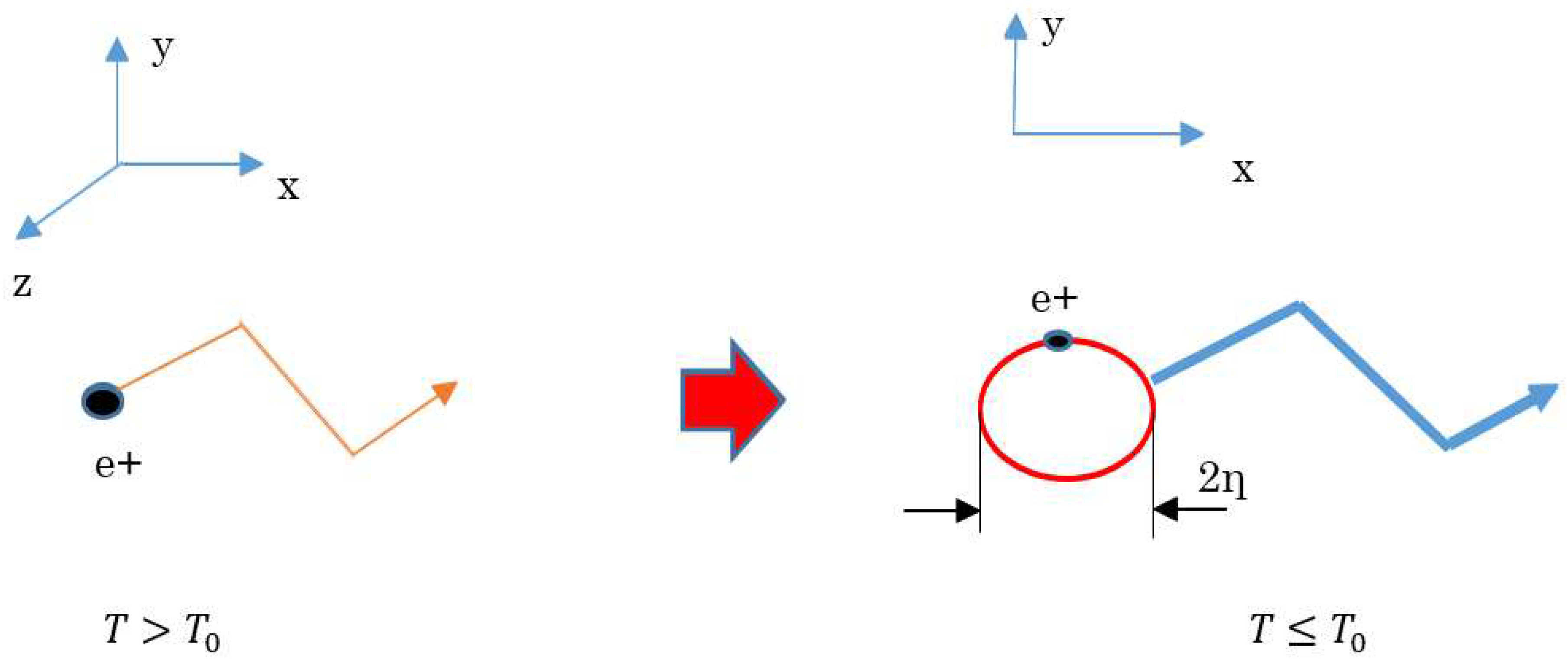
Figure 2.
Schematic of our established model to handle many-body interactions. Considering the nature of many-body interactions, note that temperatures are locally different. However, this model claims that in the differential number dN (a macroscopic Boson takes the center and dN takes a temperature ), a thermal equilibrium can be assumed. Therefore, a balance between force of expansion from Coulomb interactions, in addition to the magnetic field interactions from the Bosons and force of compression from immediate outer side, which is equal to the kinetic energies in dN (i.e., a temperature ), is formed. Calculating this balanced equation results in a new statistical equation.
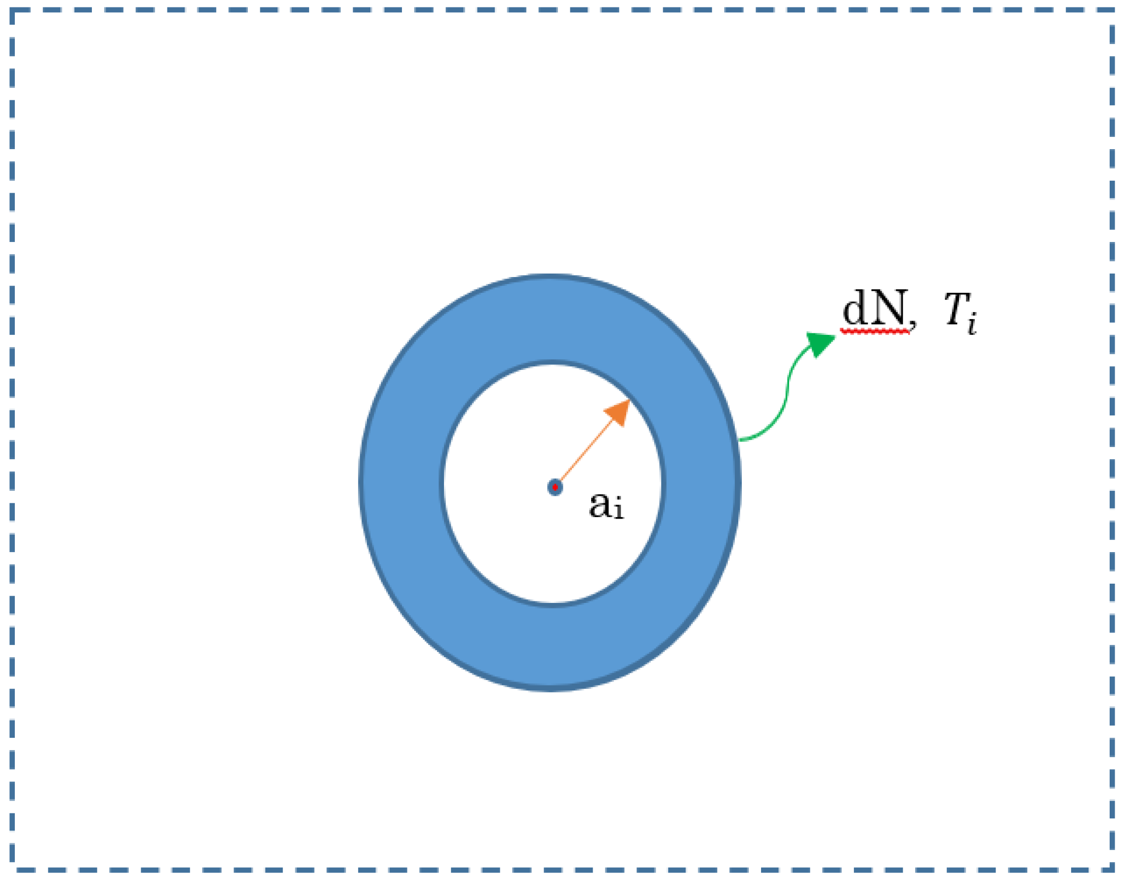
Figure 3.
A basic model of infinite well-potential. This model is directly related to the immediate prior figure model. The diameter 2 varies depending on a temperature . A macroscopic Boson in this well-potential forms a stationary wave, and its wave function and eigenvalue are presented in every basis texts. An important point is that all of these depend on index i.
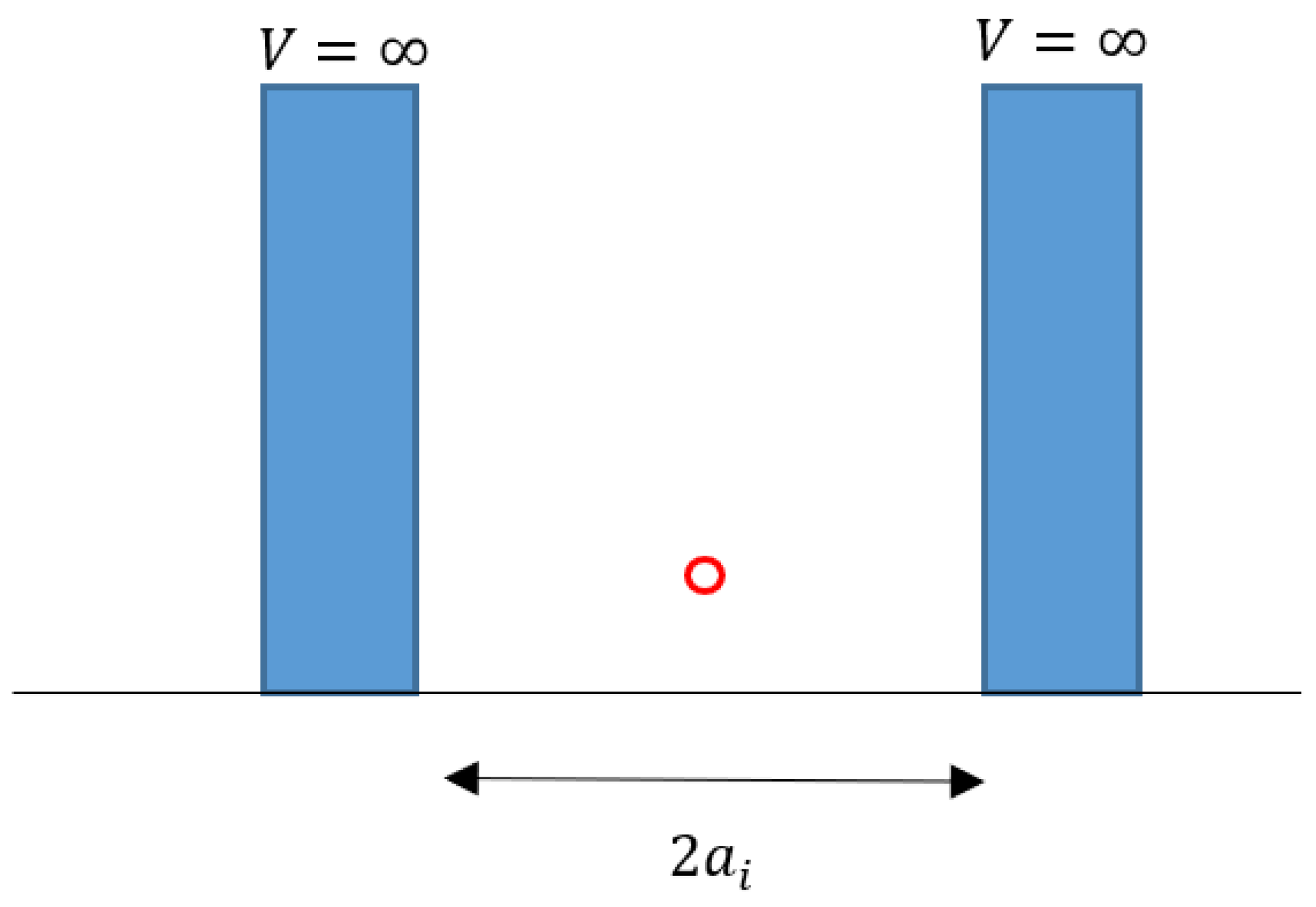
Figure 4.
Schematic of two macroscopic Bosons having many-body interactions. The relative distance of indicates one between two macroscopic Bosons. When an attractive force F between them appears and because the relative kinetic energy becomes 0, indexes i and j take the same. Thus, a superposition between them occurs, rendering be 0. That is, two Bosons now combine to be a Cooper pair. Employing the statistic equations from our established model, we can predict this type of transition.

Figure 5.
(a) Currents in the same direction. (b) Shorter leads with currents in the same direction. (c) Holes with same direction and equal velocity. (d) Center-of-mass motion of Cooper pair.
Figure 5.
(a) Currents in the same direction. (b) Shorter leads with currents in the same direction. (c) Holes with same direction and equal velocity. (d) Center-of-mass motion of Cooper pair.
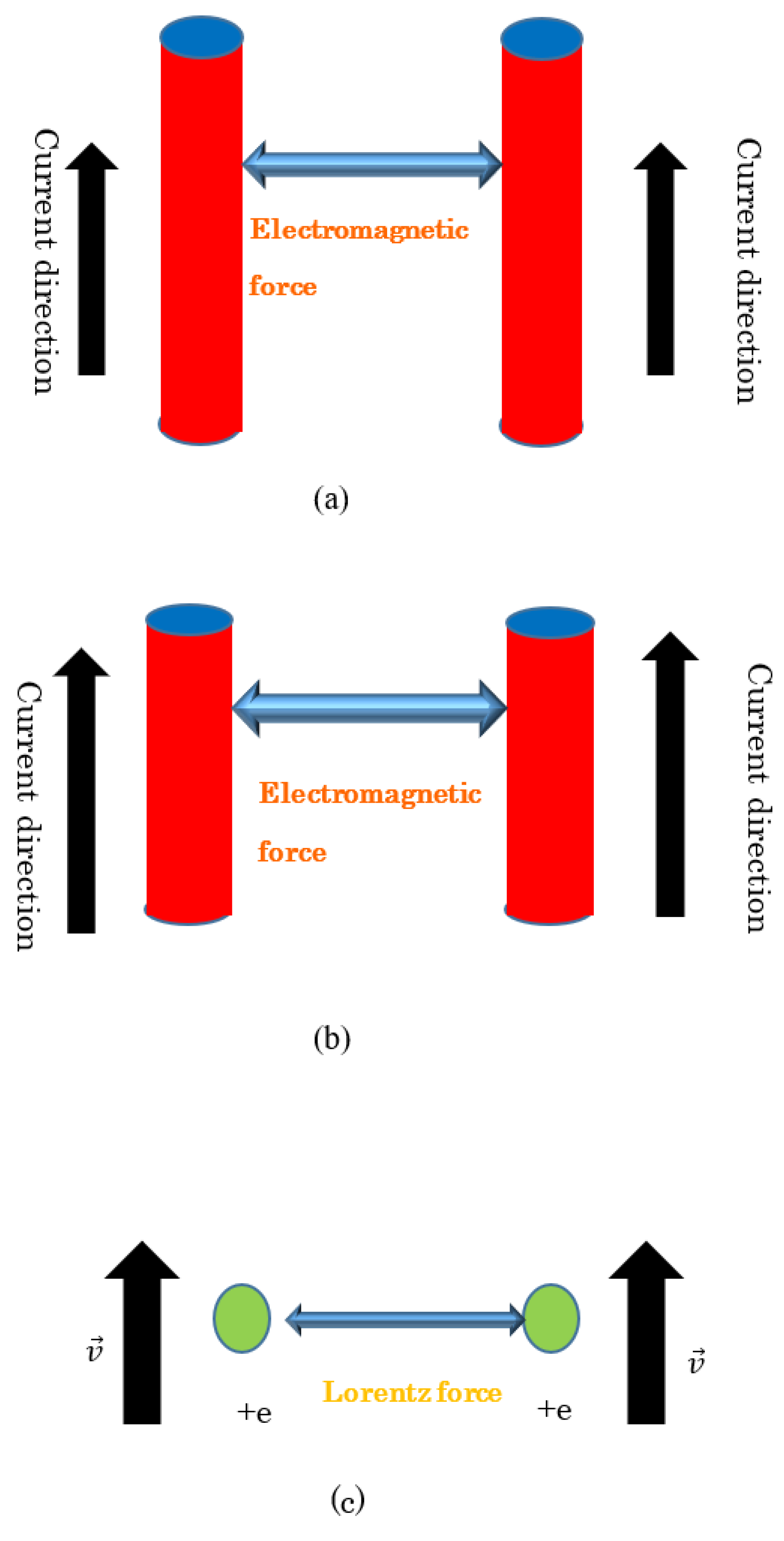
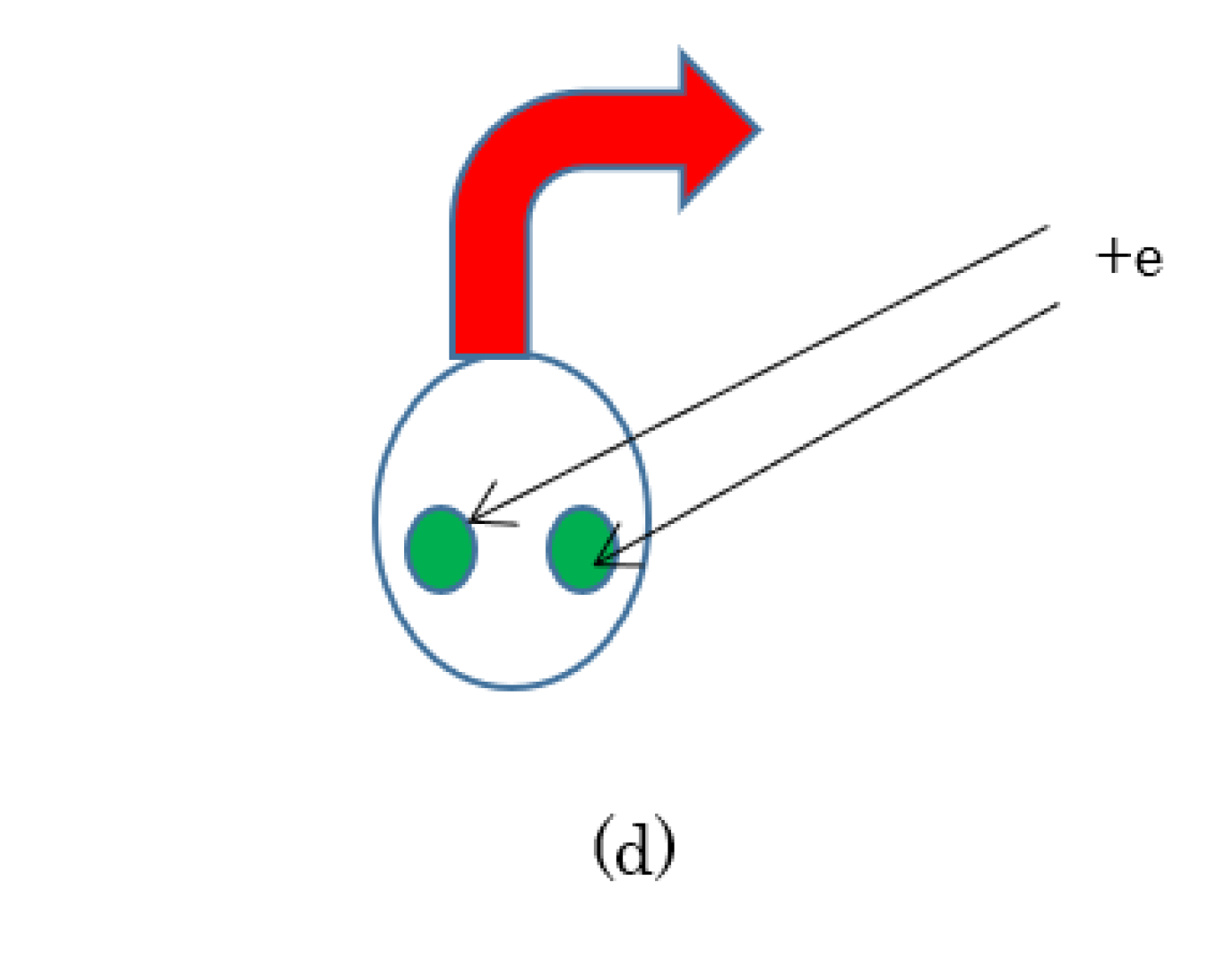
Figure 6.
A result of typical critical temperature on doping. This is derived from the equation by combining pseudo-gap energy and superconducting energy gap. At doping 0.16, the critical temperature reaches the maximum, which agrees with the experiments. In calculations, no numerical calculations or fitting method are employed. The values of critical temperatures are relatively sensitive for Debye temperature and band gap in our derived equation. This indicates that, although high-Tc cuprates in common have CuO2 surfaces, differences of Debye temperatures and band gaps would result in various values of critical temperatures among high-Tc cuprates.
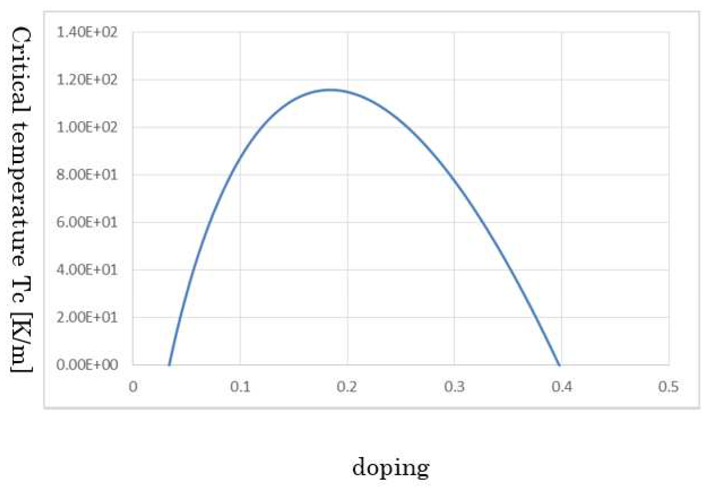
Figure 7.
The complete depiction from theoretical calculations of Tc, T*, and T0 vs. doping. Note that the horizontal axis is . For the previous figure of Tc graph, T* and T0 are added. Note that T* is depicted on the understanding that it is smaller than T0. Moreover, T* has the gradual and easy minimum point on touching Tc dome. Thus, it does not exist in the Tc dome. As mentioned, no numerical calculations and fitting methods are employed. T0 begins with about 500 K and vanishes almost at the same doping at which Tc disappears. As mentioned in the text, this transition temperature is important when considering the anomaly metal phase.
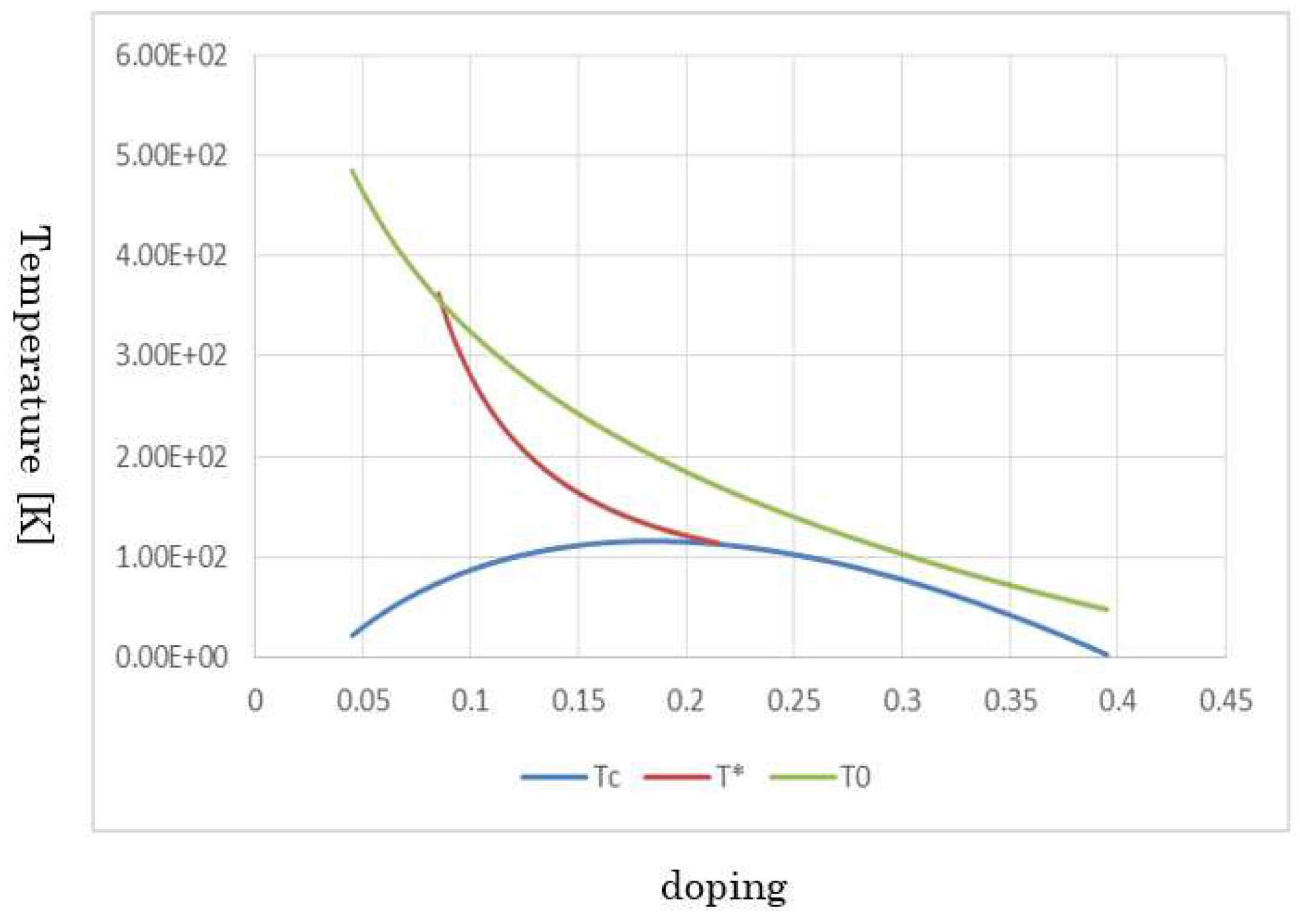
Figure 8.
Hall-effect coefficient RH on both temperature and doping. As reported in many experimental papers, lowering the doping dose arises the RH. The calculated values generally agree with experiments and that temperate dependence is non-linear.
Figure 8.
Hall-effect coefficient RH on both temperature and doping. As reported in many experimental papers, lowering the doping dose arises the RH. The calculated values generally agree with experiments and that temperate dependence is non-linear.
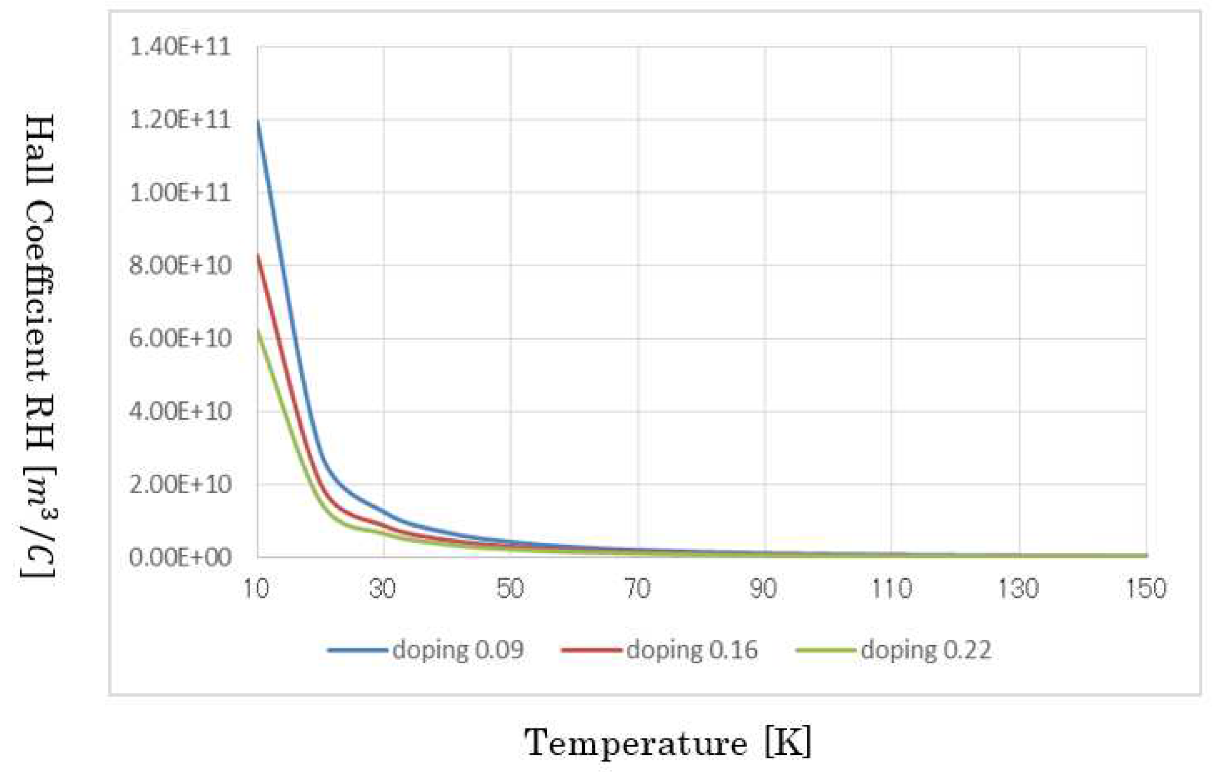
Figure 9.
A theoretical result of electron specific heat coefficient on doping. At the relatively high doping, the curve takes the maximum, which agrees with the experiments. In other words, to both lower doping or higher doping from this the maximum, electron specific heat coefficient decreases.
Figure 9.
A theoretical result of electron specific heat coefficient on doping. At the relatively high doping, the curve takes the maximum, which agrees with the experiments. In other words, to both lower doping or higher doping from this the maximum, electron specific heat coefficient decreases.
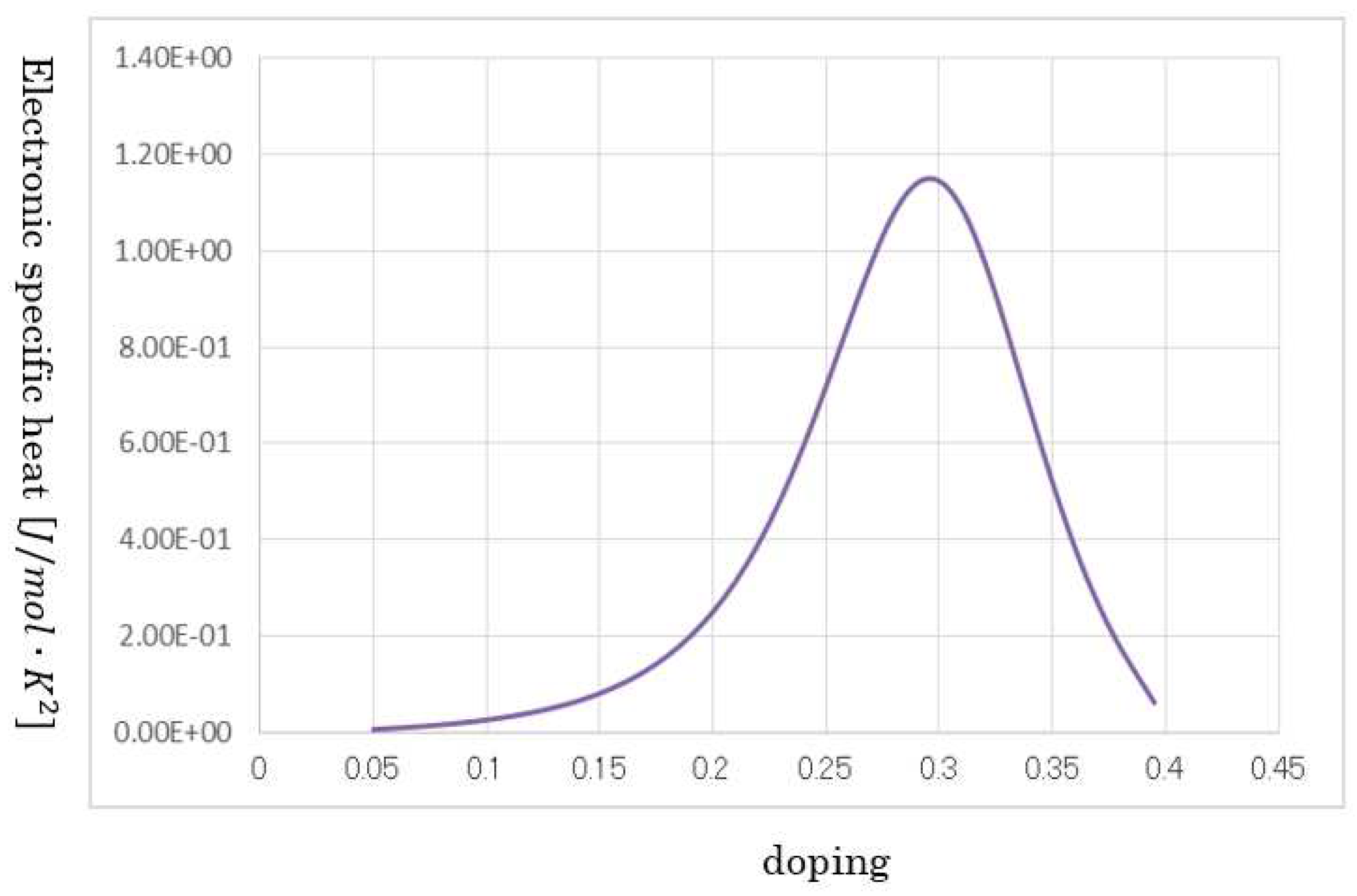
Figure 10.
Relative distance between two macroscopic Bosons versus temperature. Because, up to about 140 K, relative distances s not defined according to our statistic equation to handle the many-body interactions, up to about 140 K, the net coherence of two holes is defined as about 1 nm, i.e., superconductivity state is maintained. However, at higher temperatures, relative distances suddenly becomes order. Obviously, a transition occurs at around 140 K. As an important notation, the magnetic field interaction UB is substituted by the pseudo-gap energy at the optimum doping of 0.16. Thus, as many researchers claim, the many-body interactions in terms of macroscopic Bosons (not holes) is one of the reasons why high-Tc cuprates exhibit extremely high critical temperatures.
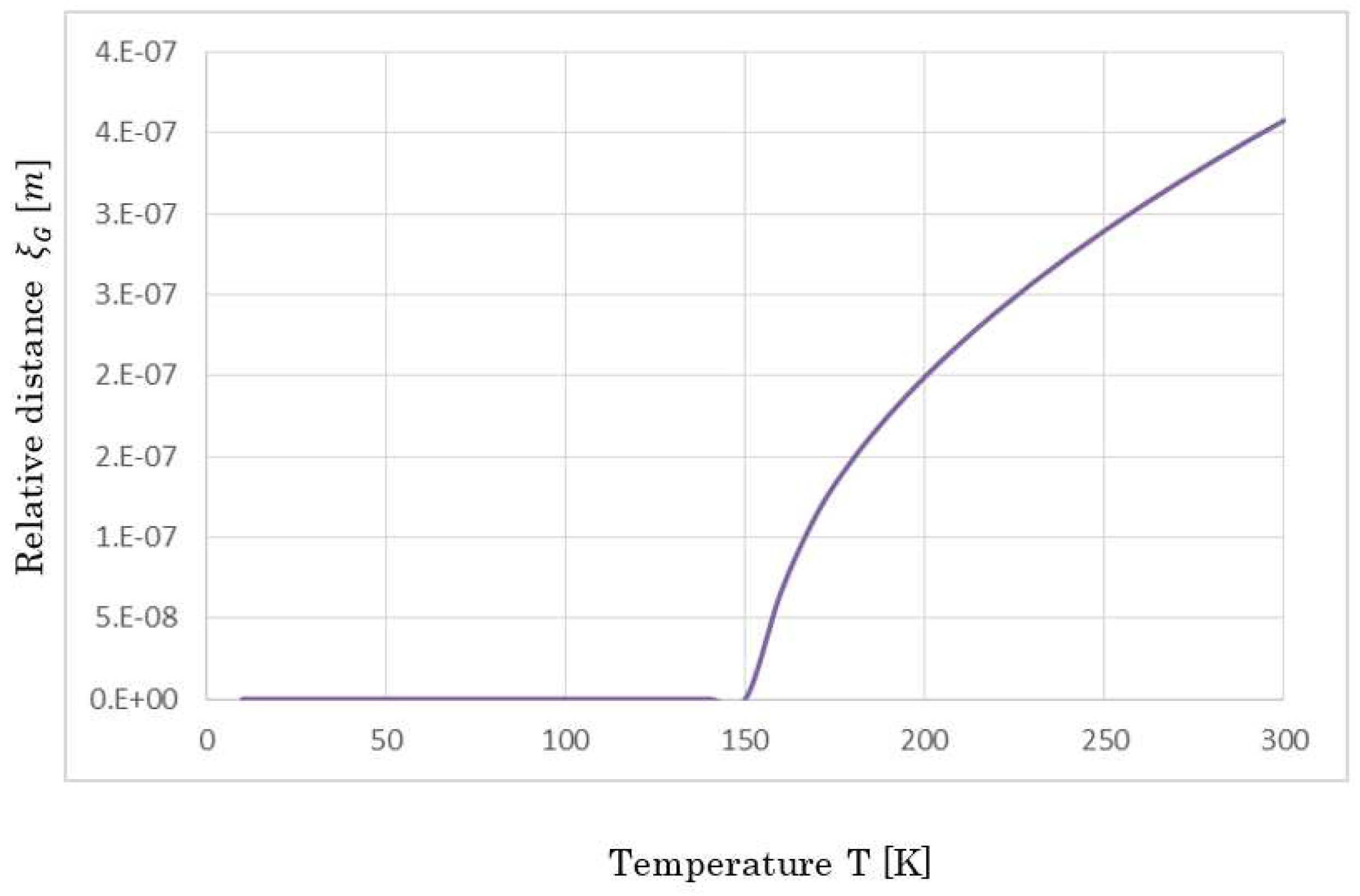
Figure 11.
Schematic of paring symmetries. The principle to generate an attractive force between two charged particles is that relative momentum must be equal. That is, when this principle is satisfied and if outer macroscopic heat energy does not disturb, the two charged particles between a long distance are combined by the generated attractive force, which stems from the Lorentz force. The above figure illustrates this principle, i.e., s-wave and d-wave symmetries. This is why there is another irrelevant particle among force–experiencing two particles. This irrelevant charged particle with different momentum does not experience this attractive force. However, the Coulomb interactions does not have this characteristic.
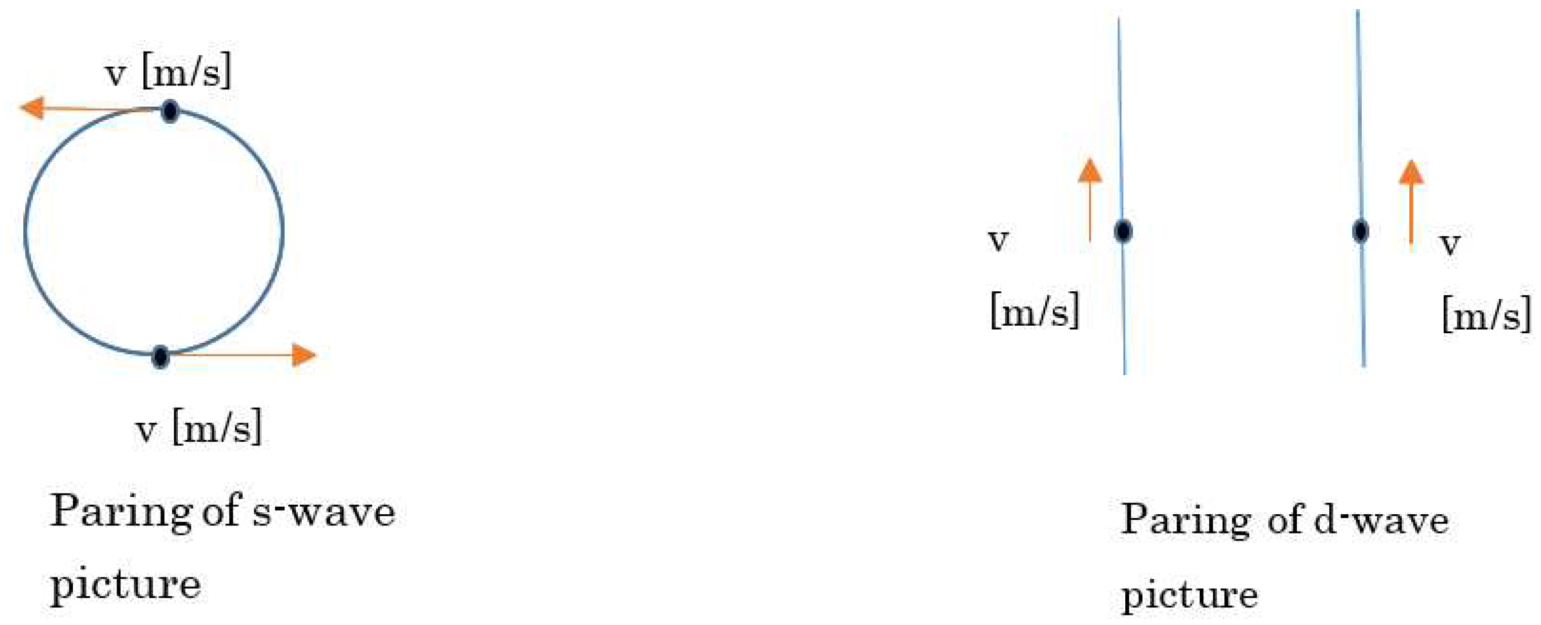
Figure 12.
The maximum Tc,max for optimum doping vs. the radius of a macroscopic Boson η. Of note, the parameter η depends on a lattice constant. As shown, Tc,max is very sensitive for parameters η. This indicates that, among high- Tc cuprates, varying substances renders their maximum critical temperatures to be variable. Moreover, it is important to recognize that Tc,max is essentially equal to the pseudo-gap at maximum doping.
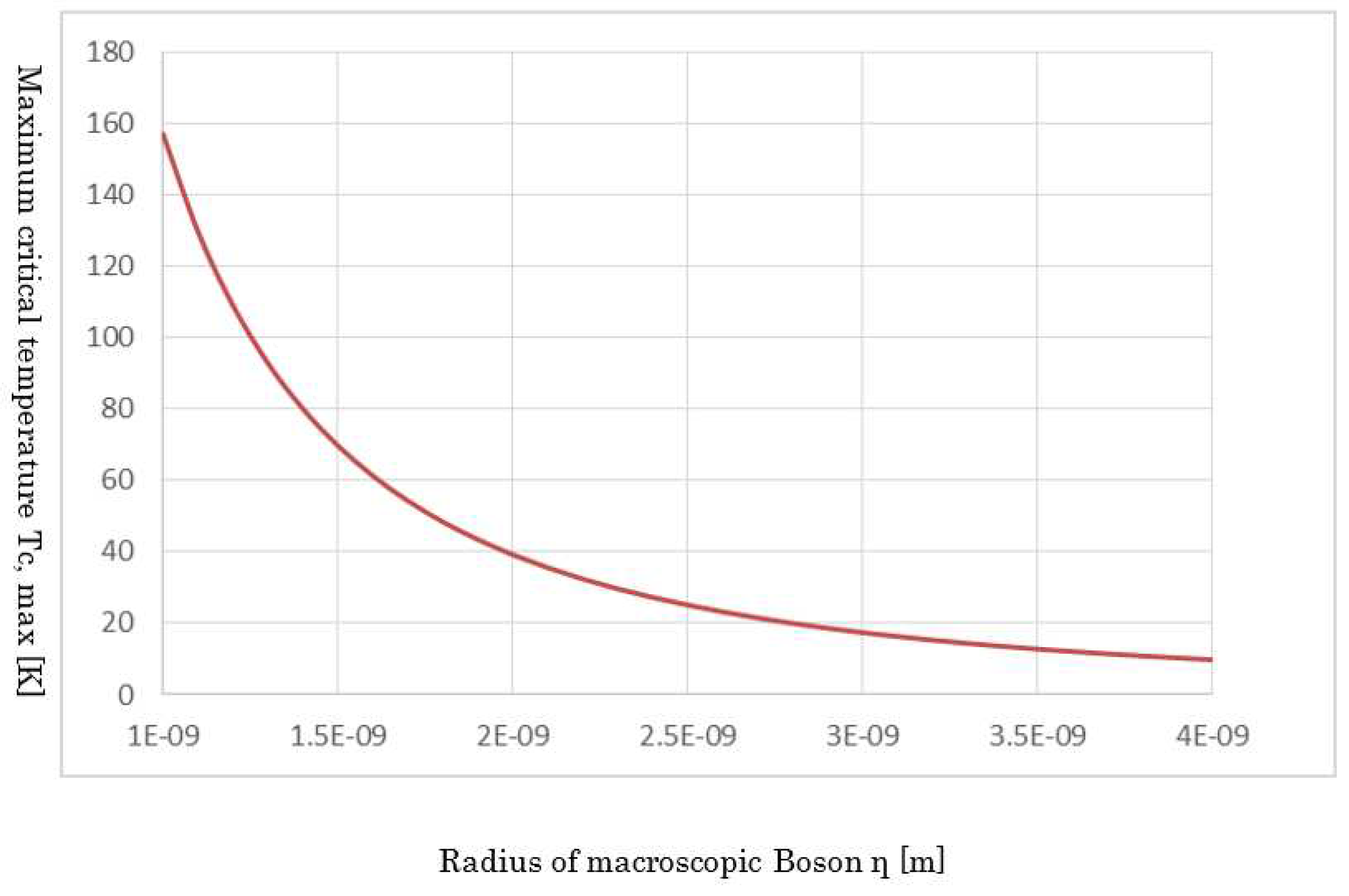
Figure 13.
Schematic of a macroscopic Boson.
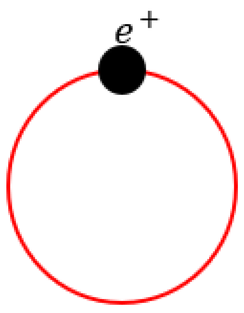
Figure 14.
Schematic of paring of two macroscopic Bosons (i.e., the two holes).
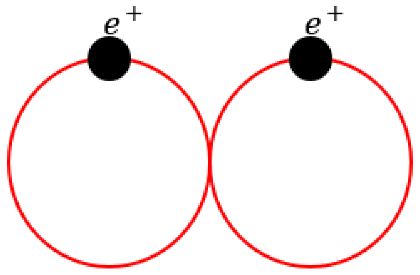
Figure 15.
Translation of the aforementioned Figure 14.
Figure 15.
Translation of the aforementioned Figure 14.
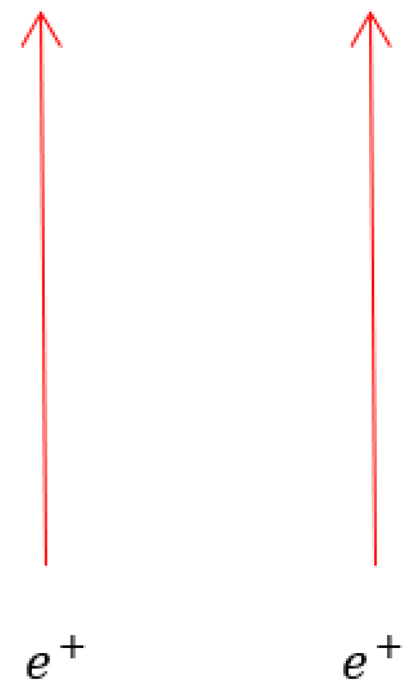
Table 1.
Physical parameters in the equation of critical temperature.
| 113.5 K | |
|---|---|
| Coherence ξ | 1 nm |
| Band gap EG | J |
| The number of layer nq | 3 |
Table 2.
Physical constants in the obtained equations.
| Debye temperature | 113.5 K |
| Coherence ξ | 1 nm |
| Band gap EG | J |
| The number of layer nq | 3 |
| Boltzmann constant kB | |
| Magnetic permeability in vacuum μ0 | |
| Electron mass m | kg |
| Electric charge of an electron e or q | |
| Radius of a macroscopic Boson η | |
| Planck constant 1 h | |
| Planck constant 2 ħ | |
| Fine structure constant α | |
| Avogadro constant | |
| Permittivity in vacuum ε0 | |
| Universal gas constant R | 8.31 |
Disclaimer/Publisher’s Note: The statements, opinions and data contained in all publications are solely those of the individual author(s) and contributor(s) and not of MDPI and/or the editor(s). MDPI and/or the editor(s) disclaim responsibility for any injury to people or property resulting from any ideas, methods, instructions or products referred to in the content. |
© 2023 by the authors. Licensee MDPI, Basel, Switzerland. This article is an open access article distributed under the terms and conditions of the Creative Commons Attribution (CC BY) license (http://creativecommons.org/licenses/by/4.0/).
Copyright: This open access article is published under a Creative Commons CC BY 4.0 license, which permit the free download, distribution, and reuse, provided that the author and preprint are cited in any reuse.


