

Submitted:
17 November 2026
Posted:
18 November 2026
You are already at the latest version
Abstract
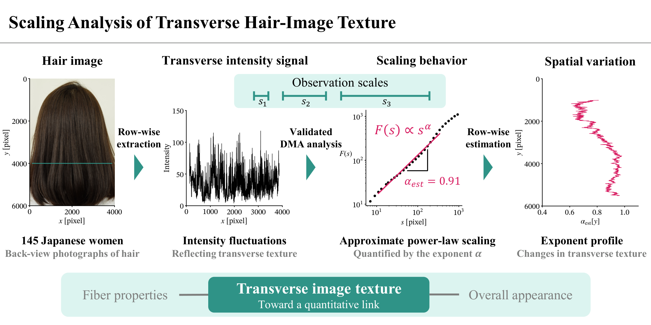
Hair appearance reflects the organization of fibers and bundles across spatial scales, but quantitative descriptions of this organization remain limited. We examined the scale dependence of transverse hair-image texture using detrending moving average (DMA) analysis of back-view photographs of 145 Japanese women. We used synthetic images to assess the effects of signal length, orientation, and spatial heterogeneity and to guide the choice of analysis conditions. Across many participants and hair regions, fluctuation functions exhibited approximate power-law scaling over the finite range analyzed. Most DMA exponents were within 0.5 < \( \alpha_{\mathrm{est}} \) <1.0, and larger exponents were associated with visually coarser textures. Among 86 participants whose hair tips were visible, exponent profiles differed substantially between individuals, while the population mean showed systematic variation from the crown toward the hair tips. DMA(0) and DMA(2) yielded broadly similar results, with local discrepancies in regions with strong spatial variation in image intensity. These findings identify a statistical relationship between fine- and coarse-scale intensity fluctuations, providing a basis for investigating hair appearance across scales. Future studies linking scaling properties to physical measurements and visual assessments could support evaluation of changes induced by products and hairdressing techniques.
Keywords:
hair texture
; image analysis
; scale dependence
; spatial scaling analysis
1. Introduction
Achieving a desired hair appearance is one of the main objectives of hair science. Hair appearance is determined not only by the morphology and color of individual fibers but also by their spatial arrangement within a fiber assembly. Hair research has primarily focused on two levels: the properties of individual fibers and the appearance of fiber assemblies. At the fiber level, studies have examined morphology, surface characteristics, and mechanical, chemical, and optical properties [2,3,4], whereas at the assembly level, luster, fiber orientation, and volume have been evaluated [5,6,7,8,9]. However, studies linking these two levels remain limited, and the contribution of individual fiber properties to the overall appearance of hair remains incompletely understood [10,11,12,13,14,15]. A quantitative description of how fibers are organized into assemblies is needed to advance this understanding.
In this study, we describe this organization in terms of spatial scale. Here, scale refers to the spatial extent over which features are examined. At small scales, the focus is on fine, local features, whereas at large scales, the focus is on the coarse features that emerge from their aggregation. Hair is a complex assembly of approximately 100,000 fibers and shows visible bundles at multiple spatial scales (Figure 1). Individual fibers form small bundles, which in turn form larger bundles, with this organization recurring across progressively larger spatial scales. A key aspect of this organization is how neighboring fibers group together in the direction transverse to their length. Examining this transverse organization at different scales may therefore help characterize how fibers form bundles of different sizes.
Scaling analysis may provide a quantitative framework for this purpose by examining how a quantity characterizing an object (a measure) varies with scale. Let s denote the scale and the measure evaluated at that scale. One form of this dependence is a power law, , which has been documented in diverse natural structures and fluctuations, including coastline geometry and heartbeat dynamics [16,17]. When this relationship holds over a given range, doubling s changes by a factor of . The scaling exponent thus summarizes the relationship between measurements at different scales, rather than the value of a measurement at a single scale.
Intuitively, a scaling exponent characterizes the roughness of a signal or texture. In cosmetic science, fractal dimensions—which are related to scaling exponents—have been estimated from image intensity or surface height to characterize skin appearance and the surface roughness of skin and individual hair fibers [18,19,20]. We previously reported a preliminary application of scaling analysis to hair as a fiber assembly [1]. The present study provides a detailed methodological description and systematic validation that were not included in that report.
Here, we examine the scale dependence of image intensity fluctuations to characterize hair-assembly texture. Using back-view photographs of Japanese women’s hair, we focus on transverse texture, which may provide clues to how neighboring fibers and bundles are organized across spatial scales. Horizontal intensity signals approximately perpendicular to the predominant fiber orientation can reflect the hierarchical hair-bundle patterns described above. Specifically, these signals exhibit fine fluctuations associated with fibers and thin bundles, together with more slowly varying fluctuations associated with wider bundle patterns (Figure 4). This analysis characterizes not only signal roughness but also how the fine- and coarse-fluctuations are related over the analyzed range of spatial scales. Furthermore, because hair texture typically changes from the crown toward the hair tips, we repeat the analysis row by row from the top to the bottom of each image to examine spatial variation in transverse scaling properties along the hair-length direction.
However, image intensity patterns cannot be directly equated with fiber arrangement. Photographs record light from a three-dimensional hair assembly as a two-dimensional image. Image intensity therefore reflects not only fiber arrangement but also illumination conditions, shading due to head shape, specular reflection, and variations in hair pigmentation. These factors can introduce intensity trends that vary more slowly across the image than the local fluctuations associated with fibers and thin bundles. Reducing these slowly varying trends helps limit their influence when assessing texture fluctuations associated with fiber arrangement. For this purpose, we use detrending moving average (DMA) analysis, which quantifies fluctuations after removing local trends [21]. Because detrending does not necessarily isolate the contribution of fiber arrangement, the estimated exponents should be interpreted primarily as characteristics of image texture; their relationship with the physical arrangement of fibers requires independent validation.
The analysis conditions themselves can also introduce biases into exponent estimation. To distinguish these effects from texture-related differences, we validate the method under controlled conditions, focusing on three factors particularly relevant to real hair images:
- Finite signal length: Image resolution and the width of the hair region constrain the length of each transverse intensity signal. This limits the range of scales that can be examined and the amount of information available at large scales.
- Variations in fiber orientation: Local fiber orientation varies, so horizontal sampling is not always perpendicular to the fibers. Such deviations may influence the intensity fluctuations and their estimated scaling exponents.
- Spatial heterogeneity: Texture properties may vary even within a single horizontal row. A single exponent may therefore conceal local differences in scaling behavior.
Synthetic images with known scaling properties allow us to assess how these factors affect the estimated exponents and to identify the conditions and limits within which the exponents can be interpreted as characteristics of hair-image texture.
In summary, this study examines whether transverse image intensity fluctuations exhibit approximate power-law scaling over a finite range and how the estimated exponents differ among individuals and vary from the crown toward the hair tips. These analyses provide a basis for investigating relationships between fine- and coarse-scale features of hair-image texture.
2. Materials & Methods
2.1. Dataset
The dataset comprised back-view photographs of the hair of 145 Japanese women aged 19–74 years, all of whom provided written informed consent before participation. The mean age was 45.1 years, with a standard deviation of 13.9 years. To capture hair in its natural condition, participants were instructed to refrain from using hair products or styling tools on the day of photography. Images were acquired using a Nikon D5300 camera (Nikon Corporation, Tokyo, Japan) at a fixed distance under standardized lighting conditions, with a resolution of pixels and 24-bit color depth. The spatial resolution was approximately 0.06 mm/pixel, close to the typical hair-fiber diameter of 0.06–0.1 mm [22,23], although individual fibers were not fully resolved. Representative images are shown in Figure 2.
2.2. Detrending Moving Average Algorithm
DMA analysis reduces the influence of slowly varying trends and examines how the magnitude of fluctuations changes with temporal or spatial scale [21,24]. The detailed algorithm is provided in Appendix A.1; the five main steps applied to each transverse intensity signal are outlined below:
- Integration: The mean intensity was subtracted, and the resulting signal was cumulatively summed to obtain an integrated signal.
- Trend estimation: A polynomial of order m was fitted locally to the integrated signal within a moving window of width s pixels to estimate the trend; this window width defines the analysis scale.
- Detrending: The estimated trend was subtracted from the integrated signal to obtain residual fluctuations.
- Calculation of the fluctuation function: The root mean square of the residuals was calculated as , representing the magnitude of the detrended fluctuations at scale s.
- Log–log fitting: Steps 2–4 were repeated at different scales, and a straight line was fitted to as a function of over the selected range.
A linear relationship in the log–log plot corresponds to power-law scaling,
where the DMA exponent describes how rapidly the magnitude of the detrended, integrated fluctuations increases with scale. Its estimate, , is the fitted slope. The coefficient of determination, , describes how closely the log–log data follow the fitted line over the analyzed range. Both quantities characterize only the selected finite range of scales, not the entire range of scales present in the image.
For both synthetic-image validation and real hair-image analysis, the fitting range was
where N is the length of the analyzed intensity signal. Higher-order DMA introduces scale distortion through polynomial detrending; is the correction factor for this distortion, with , , and [25]. The lower limit reduces the influence of short-scale effects, including local variations in fiber orientation, whereas the upper limit maintains statistical reliability at large scales.
Figure 3 illustrates the visual meaning of the DMA exponent using fractional Gaussian noise (fGn), parameterized by the Hurst exponent H [26]. For fGn, the DMA fluctuation function follows the power-law scaling in Equation (1), with . Despite having the same mean and variance, the example signals differ in visual roughness: smaller exponents produce finer, more rapidly alternating fluctuations, whereas larger exponents produce coarser, more gradually varying features. The connection between the DMA exponent and long-range spatial correlations is explained in Appendix A.2. This example illustrates scale-dependent texture without assuming that fGn reproduces the physical structure of hair.
Hereafter, DMA(m) denotes DMA analysis with local trends estimated using a polynomial of order m. DMA(0) uses a locally constant trend (a moving average), whereas DMA(2) and DMA(4) use quadratic and quartic trends, respectively. All three orders were used in the synthetic-image validation. For real hair images, we compared DMA(0) and DMA(2) to assess whether the estimated DMA exponents were consistent across detrending orders.
2.3. Validation of DMA Analysis
To validate DMA estimation, we used synthetic images with a prescribed spectral exponent , which describes how the signal power varies with spatial frequency f: . For these power-law signals, the spectral exponent and DMA exponent are theoretically related as follows [27]:
Using Equation (3), we converted the DMA estimates to spectral exponent estimates .
Test images with known spectral exponents were generated by Fourier filtering [28,29] to evaluate the effects of signal length, fiber orientation, and spatial heterogeneity. The central row of each image was analyzed using DMA(0), DMA(2), and DMA(4), with 128 realizations per condition. The mean of was compared with the prescribed exponent, or its central value under heterogeneous conditions, to assess estimation bias, while the standard deviation quantified variability across realizations. The generation procedure and validation parameters are described in Appendix B.
2.4. Extraction of Hair Regions and Transverse Intensity Signals
Images were preprocessed to isolate the hair region. Hair-region probability maps were obtained using a pretrained segmentation model [30], smoothed with a pixel Gaussian filter, and thresholded at 0.5. The standard deviation of the Gaussian kernel was set automatically from the kernel size (OpenCV, sigmaX=0), giving approximately 90.5 pixels. The binary masks were eroded with an pixel kernel for 25 iterations. Rows containing non-hair features were excluded by visual inspection. Rows in which the hair region consisted of multiple disconnected intervals were also excluded. Based on the validation results described in Section 3.1, only rows with a contiguous hair region at least 2048 pixels wide were included in the analysis. Color images were converted to grayscale using , and the mean intensity was subtracted from each extracted row signal before scaling analysis.
2.5. Implementation for Hair Images
DMA(0) and DMA(2) were applied to all eligible rows in each image. The vertical image coordinate y increases from top to bottom. For the intensity signal extracted from the row at y, the coefficient of determination and the DMA exponent were calculated. Arranging these estimates along the vertical coordinate yielded the coefficient-of-determination profile and the DMA exponent profile .
For the fitting range in Equation (2), a reference signal length of 2048 pixels at approximately 0.06 mm/pixel corresponds to window widths of approximately 0.6–12.3 mm for DMA(0) and 1.2–23.7 mm for DMA(2). Expressed in the corrected scale , both ranges correspond to approximately – mm. The upper fitting limit increased with row length, so the accessible scale range differed across positions and participants.
2.6. Assessment of the Prevalence of Approximate Power-Law Scaling over a Finite Range
To assess how widely approximate power-law scaling over a finite range was observed in the hair images, the values from all analyzed rows were aggregated within each participant without retaining their spatial coordinates. The empirical cumulative distribution function (ECDF) of these values was calculated and summarized by its 5th, 50th, and 95th percentiles. The participant-specific ECDFs were then averaged with equal weight assigned to each participant to obtain the global ECDF, and its 5th, 50th, and 95th percentiles were calculated. This equal weighting prevented participants with more analyzed rows from disproportionately influencing the global summary.
2.7. Analysis of DMA Exponent Profiles
To quantify the average variation in scaling properties from the crown toward the hair tips, a population-mean profile was estimated for the 86 participants whose hair tips were visible within the images. The vertical coordinate was normalized as , where and are the uppermost and lowermost positions of the hair mask. Thus, . However, because only rows at least 2048 pixels long contributed to the regression, the observed data did not span the entire normalized interval for every participant. The population-mean profile was estimated using weighted least-squares regression with a cubic B-spline basis with six degrees of freedom and an additional intercept. The regression used the original row-wise observations without interpolating individual profiles onto a common grid. Each row from participant i was assigned a weight of , where is the number of analyzed rows for that participant, so that each participant had the same total weight. To account for dependence between rows from the same participant, a cluster-robust covariance estimator was used, with participants as clusters. Pointwise 95% confidence intervals were calculated at each position. The estimated mean profile and confidence intervals were displayed only at positions within the observed ranges of at least 50% of the 86 participants. Finally, the null hypothesis that the population-mean profile was constant across positions was evaluated using a joint Wald test of all spline coefficients.
2.8. Software and Code Availability
Image processing, DMA analysis, synthetic-image generation, statistical analysis, and visualization were implemented in Python (version 3.12.10). The current analysis environment uses NumPy (version 2.5.4) and SciPy (version 1.18.1) for numerical computation, OpenCV (opencv-python, version 5.0.0.93) for image processing, pandas (version 3.1.1) for data handling, statsmodels (version 0.15.0) with Patsy (version 1.0.3) for spline regression and statistical inference, and Matplotlib (version 3.11.2) for visualization.
The analysis code, including the analysis notebook, DMA implementation, synthetic-image generator, and figure-generation scripts, is not publicly available but is available from the corresponding author upon reasonable request. Access to participant photographs is subject to the restrictions described in the Data Availability Statement.
3. Results
3.1. Identification of Analysis Conditions and Limits
Detailed validation results and the corresponding figures are presented in Appendix C. Here, we summarize the findings that guided the selection of analysis conditions and the interpretation of exponents in real hair images.
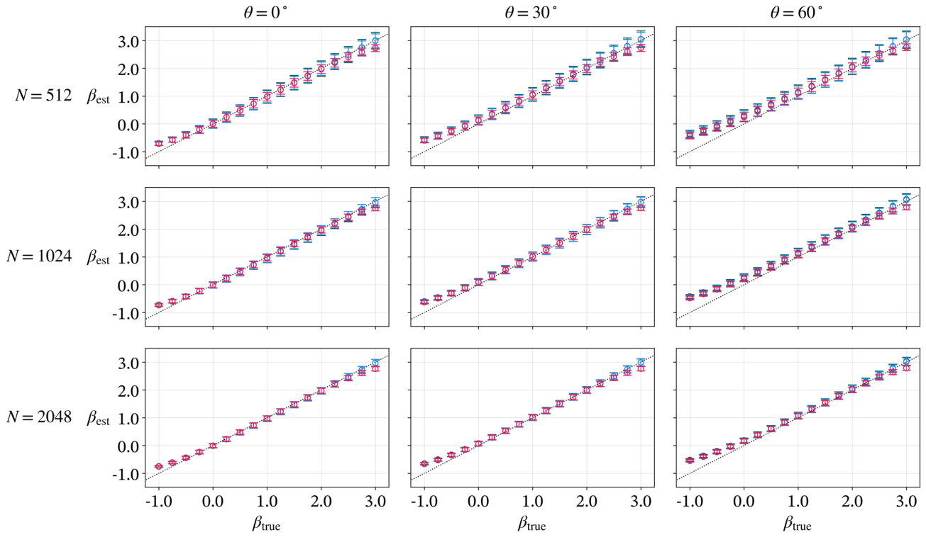
For homogeneous images with a signal length of 2048 pixels, estimates across DMA orders were generally close to the prescribed values over , corresponding to , even at an orientation angle of . Tilting the fiber orientation distorted the fluctuation function at small scales, with more pronounced distortion at higher DMA orders. The associated estimation bias was largely avoided by adjusting the fitting range to exclude the affected scales, as specified in Equation (2). Apart from this greater sensitivity to orientation at higher orders, estimation performance was broadly similar across DMA orders within this exponent range. However, when the spectral exponent varied linearly across the analyzed region, the estimates were generally close to the exponent at the center of the analyzed region but retained systematic biases that depended on both this central value and the range of spectral exponents within this region. Thus, a single exponent could summarize a central effective scaling property while concealing local heterogeneity.
These findings guided our choice to analyze only rows containing at least 2048 pixels in real hair images and to use the order-dependent fitting range in Equation (2) to reduce the effects of limited signal length and orientation. DMA(4) was not used for real images because correcting its scale distortion required larger windows without a clear improvement in estimation accuracy.
3.2. Scaling Properties of Hair Image Textures
We first illustrate the transverse intensity signals and DMA results for representative hair regions, then examine the prevalence of approximate finite-range scaling across the dataset and the spatial variation in the estimated exponents.
Figure 4 illustrates DMA analysis of transverse intensity signals extracted from upper and lower regions of a representative participant’s hair image. The upper region appeared relatively uniform, whereas wider hair bundles were visible in the lower region. The corresponding signals showed predominantly fine-scale fluctuations in the upper region and more pronounced coase-scale fluctuations in the lower region. For DMA(0), both fluctuation functions had approximately linear regions in log–log coordinates, with and , and estimated exponents of approximately and , respectively. DMA(2) gave similar estimates.
Figure 5 shows the row-wise analysis for the entire hair region of the same participant. Bundles became more visually prominent toward the lower part of the image. Both DMA orders yielded high values over most positions, indicating that approximate power-law scaling over the fitted finite range was observed across most of the analyzed hair region. DMA(2) nevertheless showed lower values than DMA(0) in some regions. The exponent profiles were similar between orders and increased from the upper to the lower region. In this example, the increase in the exponent accompanied the change toward coarser texture. Visual inspection of other images also showed a similar correspondence, with larger exponents accompanying visually coarser texture and intensity fluctuations at larger spatial scales.
Next, we examined whether approximate finite-range power-law scaling was also observed in other participants. Figure 6 shows the participant-specific distributions of row-wise values together with a global summary that gives equal weight to each participant. These distributions were concentrated near 1 for most participants, despite lower values in some images and regions. DMA(2) tended to give slightly lower values than DMA(0). The 5th, 50th, and 95th percentiles of the global ECDF were , , and for DMA(0), and , , and for DMA(2). These results support the widespread occurrence of approximate power-law scaling over the fitted finite range, while high alone does not establish scale invariance beyond that range.
Although the results were broadly consistent with approximate finite-range power-law scaling across participants, the exponent values and their spatial variation differed among individuals. Figure 7 shows the exponent profiles of the 86 participants, tracing changes in transverse scaling properties along the normalized vertical position from the crown toward the hair tips. The individual profiles, shown as thin lines, were widely dispersed, indicating substantial interindividual variation.
Most estimates were between 0.5 and 1.0, with local values reaching approximately 1.2. Under the tested signal-length and orientation conditions, synthetic-image validation showed generally accurate estimation over the wider range (Section 3.1 and Appendix C). This validated range encompasses both the predominant estimates and the local values above 1. This supports the reliability of exponent estimation under those conditions, although the estimated values alone do not reveal whether spatial heterogeneity is present within each analyzed row.
Despite the interindividual variation, the population-mean profiles, shown as thick lines, suggested an overall positional trend: for both DMA orders, the mean exponent decreased slightly in the upper observed region and then increased toward the lower region. In terms of texture roughness, these lower and higher exponents correspond to finer and coarser transverse textures, respectively. Joint Wald tests rejected the null hypothesis of a constant mean profile ( for DMA(0) and for DMA(2)), supporting variation in the population-mean exponent with normalized vertical position.
3.3. Example of Deviation from Single Power-Law Scaling
Some image regions deviated from a single scaling relationship. Figure 8 shows pronounced curvature in the log–log fluctuation functions. This image had the lowest median for DMA(0) among the analyzed images, and the selected row had the lowest within that image. Curvature was observed for both DMA orders, indicating that a single exponent did not adequately describe the selected signal. This example emphasizes the need to inspect both and the scale dependence of .
3.4. Differences Between DMA Orders
We compared the exponents estimated using DMA(0) and DMA(2) to examine the influence of detrending order (Figure 9). Estimates were generally similar across participants and hair regions. Across all valid rows pooled across participants, the mean difference was , with a standard deviation of 0.0212.
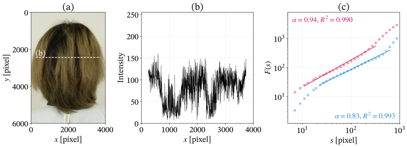
Larger differences occurred in a limited number of participants and regions. Figure 10 shows the largest discrepancy. Pronounced non-uniform coloring was accompanied by a slowly varying component in the extracted intensity signal. Although both DMA orders gave high values, their fluctuation functions and estimated exponents differed. Similar differences were observed in other regions with pronounced lateral intensity variation. Thus, the general scaling results were consistent across the two orders, while strong image inhomogeneity could affect the estimates.
4. Discussion
DMA analysis under conditions informed by synthetic-image validation revealed approximate finite-range power-law scaling in transverse hair-image texture across many participants and hair regions in the dataset of 145 Japanese women. Among the 86 participants included in the profile analysis, individual exponent profiles differed substantially, while the population mean varied systematically from the crown toward the hair tips. DMA(0) and DMA(2) yielded broadly similar results, with local discrepancies in regions with strong spatial variation in image intensity.
The main contribution of this study is the identification of a broadly observed statistical relationship across spatial scales in hair-image texture. The approximate power-law scaling indicates that fine- and coarse-scale intensity fluctuations within the analyzed range can be related through a single DMA exponent. The observed exponent range allows a more specific statistical interpretation of this behavior. Most estimates were within . If the transverse intensity signals can be regarded as approximately weakly stationary processes with power-law scaling, this range is consistent with persistent long-range spatial correlations [24,31]. As explained in Appendix A.2, this interpretation suggests that intensity fluctuations at widely separated positions remain statistically related. However, it cannot be directly extended to local estimates greater than 1. Together, these findings provide a basis for investigating how the organization of hair as a fiber assembly gives rise to local texture and large-scale patterns spanning fibers and bundles.
Power-law spatial correlations in density and mechanical properties have been reported in cross-linked fiber networks [32,33]. This conceptual parallel motivates investigating the physical organization of fiber assemblies as a possible origin of the texture scaling observed here. Hair fibers, however, are not permanently cross-linked to one another, so results from cross-linked networks cannot be applied directly to hair assemblies. Models of non-cross-linked fibers interacting through reversible adhesion resemble hair assemblies more closely in that they allow fibers to rearrange without permanent inter-fiber bonds. These models show that variations in adhesion, fiber stiffness, and density can lead to different structures, including locked configurations and connected or isolated bundles [34,35]. Such parameter-dependent organization may also contribute to the positional changes in DMA exponent profiles (Figure 5 and Figure 7). Controlled hair experiments combined with image analysis could test this possibility and help identify the physical factors underlying the observed scaling and its spatial variation.
This study may also provide a useful quantitative framework for cosmetic product development by helping investigate how individual-fiber properties and inter-fiber interactions are expressed in hair texture across spatial scales. For example, physical properties such as friction and adhesion could be measured before and after product treatment [4]. Scaling analysis could then quantify how treatment changes the statistical relationship between fine- and coarse-scale image fluctuations. Combining this description with physical measurements and independent visual assessments could help clarify how changes at the fiber level are reflected in the texture of the whole assembly and how that texture contributes to perceived hair attractiveness. If these relationships are validated, scaling properties may serve as evaluation measures to support formulation development. This approach may also be useful for examining hairdressing techniques such as haircutting, which have largely been treated empirically. Quantifying how changes in fiber length and the distribution of hair tips induced by cutting are reflected in the relationship between fine- and coarse-scale texture could help relate cutting conditions to the resulting appearance.
Several limitations should be noted. The participants were Japanese women with relatively straight to wavy hair. Although we have reported a preliminary application to other ethnic groups [1], systematic validation across ethnic groups and curl patterns remains necessary. Image intensity reflects not only fiber arrangement but also reflection, shading, and pigmentation. The estimated exponents therefore cannot be directly equated with physical structure or perceived appearance. The synthetic images did not reproduce all of these optical effects, and reproducibility across imaging conditions also requires validation. Interpretation of the power-law scaling is restricted to the finite range analyzed, and a single exponent may conceal spatial heterogeneity. Furthermore, vertical position within an image does not represent position along the length of an individual fiber. Differences in signal length, fitting range, and participant coverage across positions may also affect the estimated mean profile.
5. Conclusions
Motivated by hierarchical hair-bundle structures, this study used DMA analysis to characterize transverse hair-image texture across spatial scales, with analysis conditions informed by synthetic-image validation. Approximate power-law scaling was observed over a finite range in most participants and hair regions. Exponent profiles differed substantially among individuals, while the population mean varied systematically from the crown toward the hair tips; the main results were broadly consistent between DMA(0) and DMA(2). These findings provide a statistical basis for connecting fine- and coarse-scale features of hair-image texture. Future studies combining scaling analysis with controlled hair experiments, physical measurements, and visual assessments could clarify how fiber properties and interactions shape these relationships. Establishing these links could help guide product development and hairdressing by clarifying how changes at the fiber level affect the appearance of the hair assembly.
Author Contributions
Conceptualization, M.T. and K.K.; Methodology, M.T. and K.K.; Software, M.T.; Validation, M.T.; Formal Analysis, M.T.; Investigation, M.T.; Resources, M.T. and K.K.; Data Curation, M.T.; Writing—Original Draft Preparation, M.T.; Writing—Review & Editing, K.K.; Visualization, M.T.; Supervision, K.K.; Project Administration, M.T. and K.K. All authors have read and agreed to the published version of the manuscript.
Funding
This research received no external funding.
Institutional Review Board Statement
The study was conducted in accordance with the Declaration of Helsinki and approved by the Institutional Review Board of Brain Care Clinic (protocol number: 20171211; management number: BCC251023-3).
Informed Consent Statement
Informed consent was obtained from all subjects involved in the study.
Data Availability Statement
The data presented in this study are available on request from the corresponding author due to restrictions imposed by the ethics committee to protect participant confidentiality. Requests for access to data will be reviewed on a case-by-case basis, subject to institutional review board approval, and must align with the originally approved terms of use.
Conflicts of Interest
Author M.T. is employed by Milbon Co., Ltd. The remaining author declares no conflicts of interest.
Appendix A. Details of DMA Analysis
Appendix A.1. Detailed DMA Algorithm
DMA was implemented using a Savitzky–Golay filter, which estimates local polynomial trends by linear convolution [36,37]. Compared with detrended fluctuation analysis (DFA) [38], whose segment-wise detrending can introduce artifacts associated with segment boundaries and filter characteristics [39], the Savitzky–Golay implementation of DMA has a well-defined frequency response, providing a theoretical basis for interpreting its scale-dependent fluctuations [24].
For a zero-mean intensity signal of length N, the integrated signal was
For each evaluated odd window width s, an mth-order Savitzky–Golay filter was applied to the integrated signal by linear convolution. The filter output at each valid window center, , provided the local polynomial trend estimate. The residual was
Only positions with a complete window were retained. The fluctuation function was calculated as
Thus, measures the residual fluctuations of the integrated signal, rather than the standard deviation of the original image intensities. The calculation was repeated for all evaluated window widths. For those satisfying Equation (2), ordinary least squares was used to fit
where b is the intercept and is the regression residual. The slope gave the estimated DMA exponent, and summarized the goodness of fit in log–log coordinates.
Thirty logarithmically spaced values between 7 and approximately pixels were converted to integers. Even values were increased by one, and duplicates were removed to obtain the evaluated window widths. Only evaluated window widths satisfying Equation (2) were used for fitting. For simulation fits, the upper fitting cutoff was . The evaluated scale grid also constrained the effective upper limit for DMA(4).
Appendix A.2. DMA Exponents and Long-Range Spatial Correlations
The fGn example in Figure 3 provides a connection between the DMA exponent and spatial correlations [24,26]. For this model, . When , the autocorrelation between signal values separated by k pixels is positive and, at large separations, decays as
Because , this decay is sufficiently slow that
which defines long-range dependence in this setting. Thus, fluctuations at widely separated positions remain statistically related, even though their correlation weakens with distance. For comparison, fGn with is uncorrelated, whereas corresponds to negatively correlated fluctuations.
For hair images, exponents within are consistent with persistent spatial correlations if the transverse intensity signals can be treated as approximately stationary processes with power-law scaling. This interpretation suggests that hair texture may involve statistical relationships extending across neighboring fibers and bundles, motivating investigation of such relationships as a property of the fiber assembly. The present finite-range analysis does not establish long-range dependence at arbitrarily large separations or identify the physical fiber interactions responsible for the observed texture.
Appendix B. Synthetic-Image Generation and Validation Conditions
Appendix B.1. Image Generation
Synthetic images were generated by Fourier filtering to produce strongly anisotropic textures with prescribed spectral exponents [28,29]. Each image was first constructed on a grid, then rotated and cropped to pixels. The procedure was as follows:
- Specify the exponent profile. A row-dependent exponent , , was assigned before rotation.
- Generate a common white-noise input. A sequence , , was drawn from a standard normal distribution, and its discrete Fourier transform was calculated. The same sequence was used for every row within an image to impose strong directional structure.
-
Generate each row from the target power spectrum. The power spectrum describes how the variance of an intensity signal is distributed across spatial frequencies. Spatial frequency f is the inverse of spatial wavelength: for example, pixel−1 corresponds to a variation with a wavelength of 10 pixels. For each row, the target power spectrum waswhere , , is the spatial frequency folded about the Nyquist frequency. The Fourier coefficients were weighted asThe inverse Fourier transform of yielded the real intensity signal .
- Normalize and assemble the rows. Each row was rescaled to and arranged to form the intermediate image:
- Rotate, crop, and extract the signal. The intermediate image was rotated by about its center using bilinear interpolation, then cropped to its central region. DMA was applied to the central horizontal row. At , the predominant texture orientation is vertical and therefore perpendicular to this row.
For heterogeneous images, the pre-rotation profile was adjusted so that the prescribed spectral exponent varied linearly from to across the analyzed row after rotation and cropping. Here, is the central exponent and is the total exponent range across that row.
Appendix B.2. Validation Parameters
The full parameter grid is summarized in Table A1. The comparisons reported here use homogeneous images () to examine signal-length and orientation effects, and focus on with to examine heterogeneity effects. For each condition, 128 images were generated and analyzed using DMA(0), DMA(2), and DMA(4). The estimated exponents were converted to [27]. Their means were compared with for homogeneous images and with for heterogeneous images, and their standard deviations described variation across realizations.

Table A1.
Parameter values used in synthetic-image validation. The image size after cropping was pixels, and the analyzed signal length was N.
Table A1.
Parameter values used in synthetic-image validation. The image size after cropping was pixels, and the analyzed signal length was N.
| Parameter | Symbol | Values |
|---|---|---|
| Signal length (pixels) | N | |
| Orientation angle | ||
| Central spectral exponent | ||
| Heterogeneity width |
Appendix C. Detailed Results of Synthetic-Image Validation
The results below examine the effects of signal length, orientation, and spatial heterogeneity using 128 realizations per condition. Image generation and validation parameters are described in Appendix B.
Appendix C.1. Homogeneous Scaling Properties
Figure A1 shows images with homogeneous scaling properties (). At , all DMA orders produced approximately linear log–log plots, with slopes close to the theoretical value. Increasing the orientation angle suppressed small-scale fluctuations and produced steeper local slopes, particularly at higher detrending orders. Image discretization and smoothing introduced by rotation with bilinear interpolation may have contributed to this effect. At larger scales, the curves approached the expected behavior, indicating the importance of selecting the fitting range specified in Equation (2).
Figure A1.
Representative DMA results for synthetic images with , a central spectral exponent of , and a heterogeneity width of under different orientation angles: (a) , (b) , and (c) . Top panels show the generated images, with red lines indicating the extracted horizontal profiles. Bottom panels show log–log plots of the fluctuation function obtained using DMA(0) (red), DMA(2) (blue), and DMA(4) (green). Black dotted lines indicate the theoretical slope .
Figure A1.
Representative DMA results for synthetic images with , a central spectral exponent of , and a heterogeneity width of under different orientation angles: (a) , (b) , and (c) . Top panels show the generated images, with red lines indicating the extracted horizontal profiles. Bottom panels show log–log plots of the fluctuation function obtained using DMA(0) (red), DMA(2) (blue), and DMA(4) (green). Black dotted lines indicate the theoretical slope .
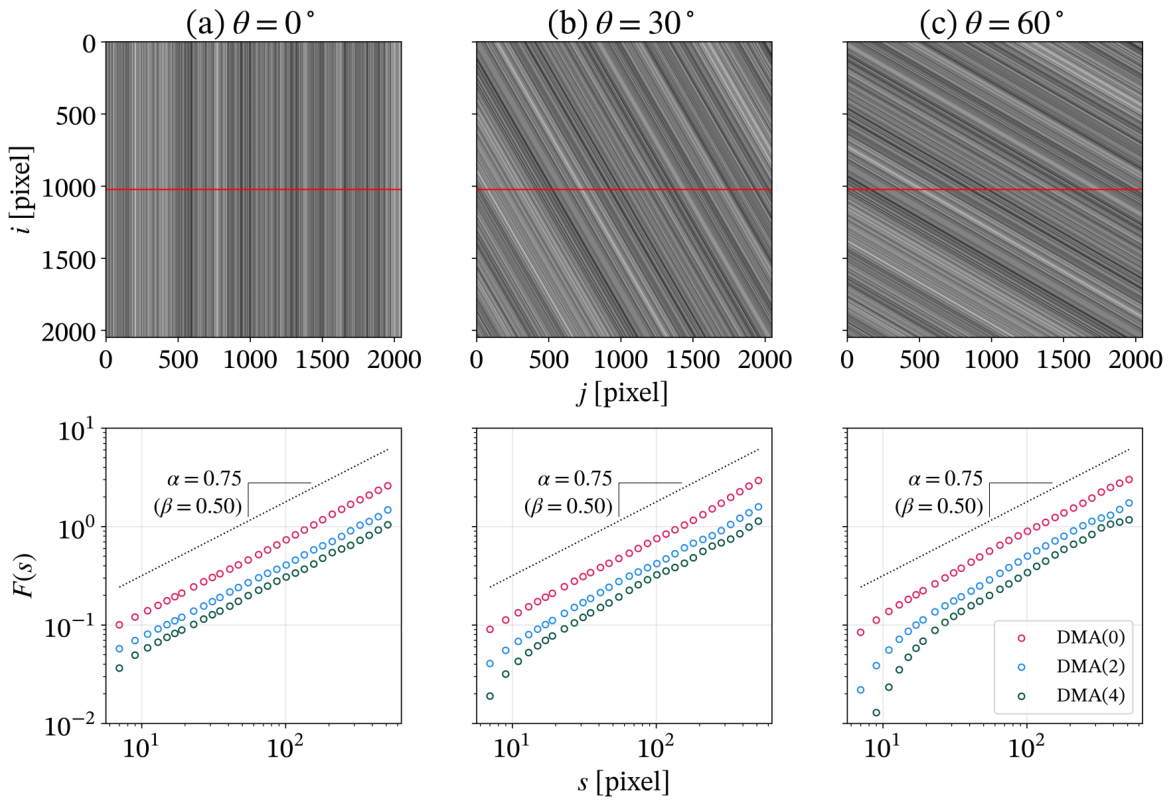
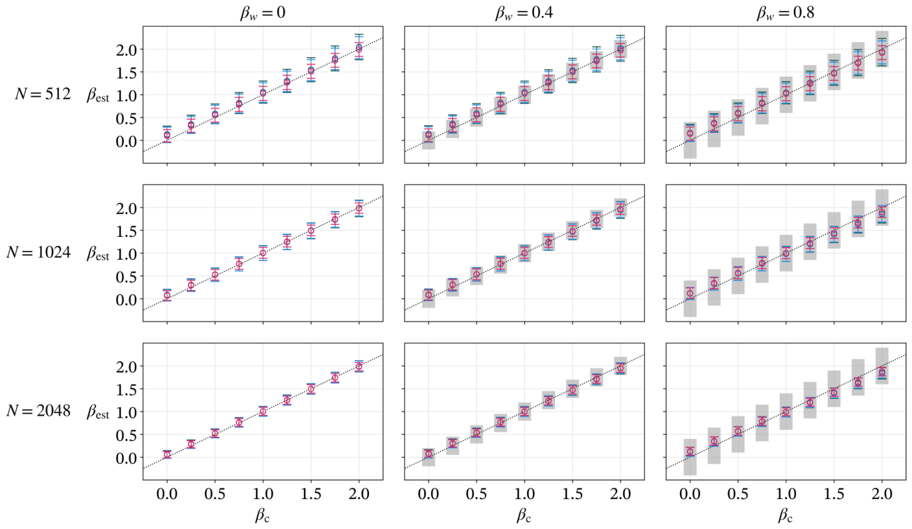
Figure A2 summarizes the homogeneous-image results. The most prominent order-dependent difference was underestimation by DMA(0) near , consistent with its theoretical estimation range , or for [31]. Other trends were broadly similar across orders. Estimates exceeded the prescribed values when , possibly in part because of finite-size effects. Larger orientation angles increased overestimation, especially at small . Longer signals generally reduced the standard deviation of estimates. With sufficiently long signals and small orientation angles, estimates were generally close to the prescribed values over .
Figure A2.
Performance of DMA for different image sizes and orientation angles. Panels are arranged by image size (rows) and orientation angle (columns). In each panel, the estimated spectral exponent is plotted against the true exponent . Markers and error bars represent the mean and standard deviation from 128 independent realizations for DMA(0) (red), DMA(2) (blue), and DMA(4) (green). The black dotted line indicates the ideal relationship .
Figure A2.
Performance of DMA for different image sizes and orientation angles. Panels are arranged by image size (rows) and orientation angle (columns). In each panel, the estimated spectral exponent is plotted against the true exponent . Markers and error bars represent the mean and standard deviation from 128 independent realizations for DMA(0) (red), DMA(2) (blue), and DMA(4) (green). The black dotted line indicates the ideal relationship .
Appendix C.2. Spatially Heterogeneous Scaling Properties
Figure A3 compares a homogeneous reference with examples in which the spectral exponent varied linearly across the analyzed row. Compared with the homogeneous reference, the fluctuation functions remained approximately linear in log–log coordinates despite the heterogeneity. Thus, apparent power-law scaling can occur even when local scaling properties are not uniform. This behavior was similar across DMA orders.
In the repeated heterogeneous-image analyses (Figure A4), estimates were generally close to the central spectral exponent . Nevertheless, overestimation was observed at and underestimation at . Increasing the spectral-exponent range amplified these biases on either side of : overestimation became more pronounced at , and underestimation became more pronounced at . Longer signals reduced the standard deviation, but systematic deviations from remained. Results were broadly consistent across DMA orders.
Figure A3.
Representative DMA results comparing a homogeneous reference with spatially heterogeneous synthetic images. All images have pixels with , a central spectral exponent of , and an orientation angle of . Top panels show (a) the homogeneous reference () and linear-gradient cases with (b) and (c) . Red lines indicate the analyzed horizontal rows. Blue lines indicate isolines of the spectral exponent . Bottom panels show log–log plots of obtained using DMA(0) (red), DMA(2) (blue), and DMA(4) (green). Black dotted lines indicate the theoretical slope .
Figure A3.
Representative DMA results comparing a homogeneous reference with spatially heterogeneous synthetic images. All images have pixels with , a central spectral exponent of , and an orientation angle of . Top panels show (a) the homogeneous reference () and linear-gradient cases with (b) and (c) . Red lines indicate the analyzed horizontal rows. Blue lines indicate isolines of the spectral exponent . Bottom panels show log–log plots of obtained using DMA(0) (red), DMA(2) (blue), and DMA(4) (green). Black dotted lines indicate the theoretical slope .
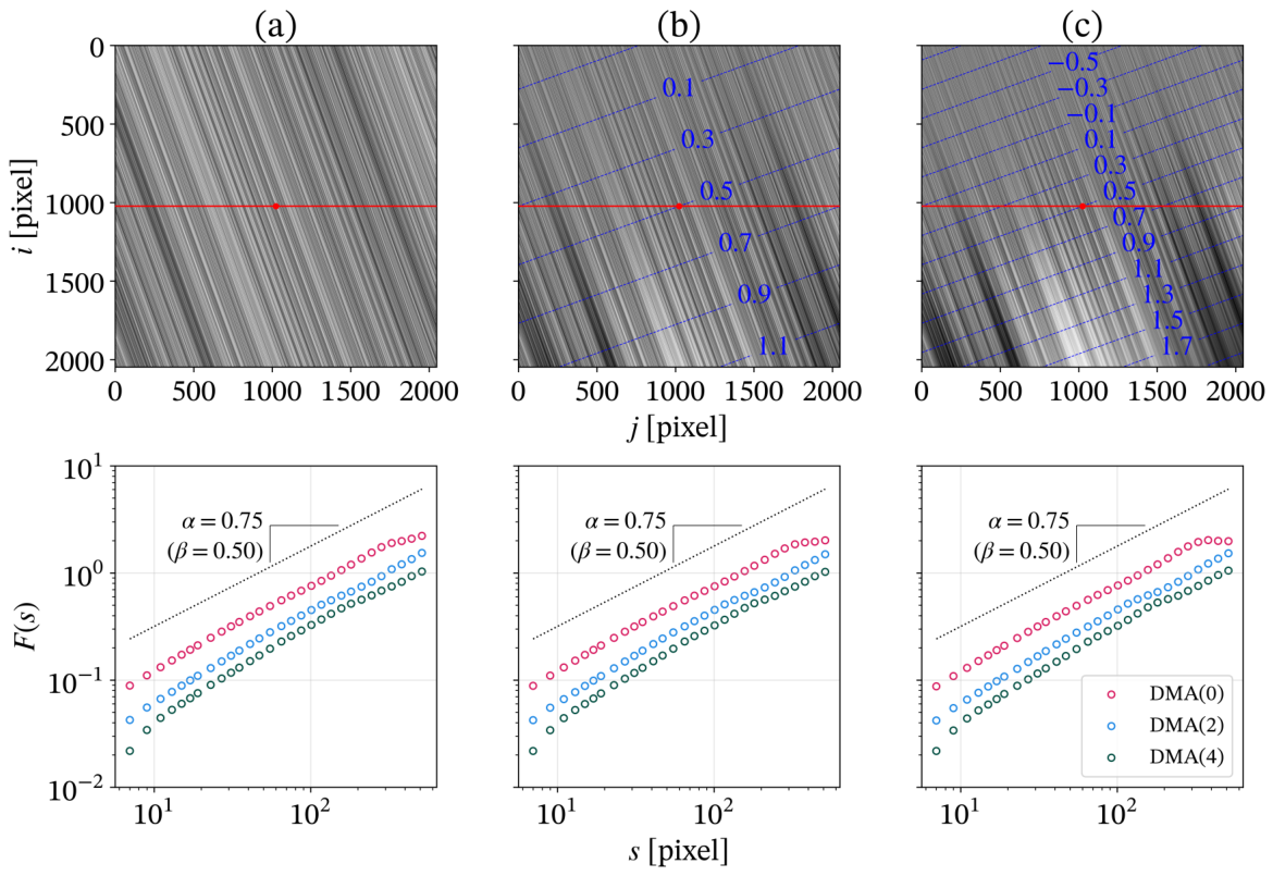
Figure A4.
Robustness of DMA against linear spatial gradients in the spectral exponent. Panels are arranged by image size N (rows) and heterogeneity width (columns). The estimated spectral exponent is plotted against the central spectral exponent . Gray shaded regions indicate the range of variation within the analysis window. Markers and error bars represent the mean and standard deviation from 128 independent realizations for DMA(0) (red), DMA(2) (blue), and DMA(4) (green). The black dotted line indicates the ideal relationship .
Figure A4.
Robustness of DMA against linear spatial gradients in the spectral exponent. Panels are arranged by image size N (rows) and heterogeneity width (columns). The estimated spectral exponent is plotted against the central spectral exponent . Gray shaded regions indicate the range of variation within the analysis window. Markers and error bars represent the mean and standard deviation from 128 independent realizations for DMA(0) (red), DMA(2) (blue), and DMA(4) (green). The black dotted line indicates the ideal relationship .
References
- Takeda, M.; Adomi, R.; Ito, L.; Kiyono, K. Universal Fractal Principle Underlying Hair Architecture: Toward a New Hair Design Paradigm. In Proceedings of the the 36th IFSCC Congress Full paper presented at the 36th IFSCC Congress, Perth, Australia, 28 September –1 October 2026. Full paper presented at the 36th IFSCC Congress, September 28–October 1, 2026. [Google Scholar]
- Robbins, C.R. Chemical and Physical Behavior of Human Hair, 5th ed.; Springer: Berlin, Heidelberg, 2012. [Google Scholar] [CrossRef]
- Evans, T.; Wickett, R.R. (Eds.) Practical Modern Hair Science; Allured Publishing: Carol Stream, IL, USA, 2012. [Google Scholar]
- Bhushan, B. Biophysics of Human hair, 1st ed.; Springer: Berlin, Heidelberg, 2010; p. 192. [Google Scholar] [CrossRef]
- McMullen, R.L. Image Analysis Tools to Quantify Visual Properties of Hair Fiber Assemblies. In Practical Modern Hair Science; Evans, T., Wickett, R.R., Eds.; Allured Publishing: Carol Stream, IL, 2012; Volume chapter 9, pp. 295–332. [Google Scholar]
- Lechocinski, N.; Breugnot, S. Fiber orientation measurement using polarization imaging. J. Cosmet. Sci. 2011, 62, 85–100. [Google Scholar] [PubMed]
- Daniels, G.; Tamburic, S.; Benini, S.; Randall, J.; Sanderson, T.; Savardi, M. Artificial Intelligence in hair research: A proof-of-concept study on evaluating hair assembly features. Int. J. Cosmet. Sci. 2021, 43, 405–418. [Google Scholar] [CrossRef] [PubMed]
- Takeda, M.; Lee, S.; Kiyono, K. Scale-robust fibre orientation analysis of hair using two-dimensional Fourier transform. Int. J. Cosmet. Sci. 2025, 48, 539–548. [Google Scholar] [CrossRef] [PubMed]
- Harrar, M.; Six, C.; Littaye, P.; Delcourt, S.; Dubois, I.; Jelidi, S.; Pouradier, F. Bridging the gap between consumer perception and objective measurements: A novel multiview image analysis methodology for quantifying hair volume on a human head (curl type I to III). Int. J. Cosmet. Sci. 2026, 00, 1–12. [Google Scholar] [CrossRef] [PubMed]
- Robbins, C.R.; Scott, G.V. Prediction of Hair Assembly Characteristics from Single Fiber Properties. J. Soc. Cosmet. Chem. 1978, 29, 783–792. [Google Scholar]
- Robbins, C.R.; Reich, C. Prediction of hair assembly characteristics from single-fiber properties. II: The relationship of fiber curvature, friction, stiffness, and diameter to combing behavior. J. Soc. Cosmet. Chem. 1986, 37, 141–158. [Google Scholar]
- Goldstein, R.E.; Warren, P.B.; Ball, R.C. Shape of a Ponytail and the Statistical Physics of Hair Fiber Bundles. Phys. Rev. Lett. 2012, 108, 078101. [Google Scholar] [CrossRef] [PubMed]
- Nagase, S.; Kajiura, Y.; Mamada, A.; Abe, H.; Shibuichi, S.; Satoh, N.; Itou, T.; Shinohara, Y.; Amemiya, Y. Changes in structure and geometric properties of human hair by aging. J. Cosmet. Sci. 2009, 60, 637–648. [Google Scholar] [CrossRef]
- Nagase, S. Hair structures affecting hair appearance. Cosmetics 2019, 6, 43. [Google Scholar] [CrossRef]
- Loussouarn, G.; Garcel, A.L.; Lozano, I.; Collaudin, C.; Porter, C.; Panhard, S.; Saint-Léger, D.; De La Mettrie, R. Worldwide diversity of hair curliness: a new method of assessment. Int. J. Dermatol. 2007, 46, 2–6. [Google Scholar] [CrossRef] [PubMed]
- Mandelbrot, B. How long is the coast of Britain? Statistical self-similarity and fractional dimension. Science 1967, 156. [Google Scholar] [CrossRef] [PubMed]
- Goldberger, A.L.; Amaral, L.A.; Hausdorff, J.M.; Ivanov, P.C.; Peng, C.K.; Stanley, H.E. Fractal dynamics in physiology: Alterations with disease and aging. Proc. Natl. Acad. Sci. USA 2002, 99, 2466–2472. [Google Scholar] [CrossRef] [PubMed]
- Haeri, M.; Phamduy, T.; Cafone, N.; Turkileri, K.; Velkov, D. Novel digital image analysis using fractal dimension for assessment of skin radiance. Skin. Res. Technol. 2019, 25, 564–571. [Google Scholar] [CrossRef] [PubMed]
- Zapletalova, A.; Pata, V.; Janis, R.; Kejlova, K.; Stoklasek, P. Objective measurements of skin surface roughness after microdermabrasion treatment. Skin. Res. Technol. 2017, 23, 346–353. [Google Scholar] [CrossRef] [PubMed]
- Zielinski, M. A New Approach to Hair Surface Topography: Fourier Transform and Fractal Analysis. J. Soc. Cosmet. Chem. 1989, 40, 173–189. [Google Scholar]
- Carbone, A. Detrending moving average algorithm: A brief review. In Proceedings of the 2009 IEEE Toronto International Conference Science and Technology for Humanity (TIC-STH), 2009; pp. 691–696. [Google Scholar] [CrossRef]
- Tajima, M.; Hamada, C.; Arai, T.; Miyazawa, M.; Shibata, R.; Ishino, A. Characteristic features of Japanese women’s hair with aging and with progressing hair loss. J. Dermatol. Sci. 2007, 45, 93–103. [Google Scholar] [CrossRef] [PubMed]
- Loussouarn, G.; Lozano, I.; Panhard, S.; Collaudin, C.; Rawadi, C.E.; Genain, G. Diversity in human hair growth, diameter, colour and shape. An in vivo study on young adults from 24 different ethnic groups observed in the five continents. Eur. J. Dermatol. 2016, 26, 144–154. [Google Scholar] [CrossRef] [PubMed]
- Kiyono, K.; Tsujimoto, Y. Time and frequency domain characteristics of detrending-operation-based scaling analysis: Exact DFA and DMA frequency responses. Phys. Rev. E 2016, 94, 012111. [Google Scholar] [CrossRef] [PubMed]
- Fujimoto, Y.; Mangalam, M.; Kiyono, K. Enhanced scaling crossover detection in long-range correlated time series. Chaos Solitons Fractals X 2025, 14, 100125. [Google Scholar] [CrossRef]
- Mandelbrot, B.B.; Ness, J.W.V. Fractional Brownian motions, fractional noises and applications. SIAM Rev. 1968, 10, 422–437. [Google Scholar] [CrossRef]
- Kiyono, K. Establishing a direct connection between detrended fluctuation analysis and Fourier analysis. Phys. Rev. E 2015, 92, 042925. [Google Scholar] [CrossRef] [PubMed]
- Chen, Z.; Ivanov, P.C.; Hu, K.; Stanley, H.E. Effect of nonstationarities on detrended fluctuation analysis. Phys. Rev. E 2002, 65, 041107. [Google Scholar] [CrossRef] [PubMed]
- Wang, Y.; Azam, A.; Wilson, M.C.; Neville, A.; Morina, A. Generating fractal rough surfaces with the spectral representation method. Proc. Inst. Mech. Eng. Part J. J. Eng. Tribol. 2021, 235, 2640–2653. [Google Scholar] [CrossRef]
- Tkachenka, A.; Karpiak, G.; Vakunov, A.; Kartynnik, Y.; Ablavatski, A.; Bazarevsky, V.; Pisarchyk, S. Real-time Hair Segmentation and Recoloring on Mobile GPUs, 2019. arXiv arXiv:1907.06740. [CrossRef]
- Carbone, A.; Kiyono, K. Detrending moving average algorithm: Frequency response and scaling performances. Phys. Rev. E 2016, 93, 063309. [Google Scholar] [CrossRef] [PubMed]
- Hatami-Marbini, H.; Picu, R.C. Heterogeneous long-range correlated deformation of semiflexible random fiber networks. Phys. Rev. E 2009, 80, 046703. [Google Scholar] [CrossRef] [PubMed]
- Picu, R.C.; Hatami-Marbini, H. Long-range correlations of elastic fields in semi-flexible fiber networks. Comput. Mech. 2010, 46, 635–640. [Google Scholar] [CrossRef]
- Sengab, A.; Picu, R.C. Filamentary structures that self-organize due to adhesion. Phys. Rev. E 2018, 97, 032506. [Google Scholar] [CrossRef] [PubMed]
- Picu, R.C.; Sengab, A. Structural evolution and stability of non-crosslinked fiber networks with inter-fiber adhesion. Soft Matter 2018, 14, 2254–2266. [Google Scholar] [CrossRef] [PubMed]
- Arianos, S.; Carbone, A.; Türk, C. Self-similarity of higher-order moving averages. Phys. Rev. E 2011, 84, 046113. [Google Scholar] [CrossRef] [PubMed]
- Tsujimoto, Y.; Miki, Y.; Shimatani, S.; Kiyono, K. Fast algorithm for scaling analysis with higher-order detrending moving average method. Phys. Rev. E 2016, 93, 053304. [Google Scholar] [CrossRef] [PubMed]
- Peng, C.K.; Havlin, S.; Stanley, H.E.; Goldberger, A.L. Quantification of scaling exponents and crossover phenomena in nonstationary heartbeat time series. Chaos 1995, 5, 82–87. [Google Scholar] [CrossRef] [PubMed]
- Kiyono, K.; Tsujimoto, Y. Nonlinear filtering properties of detrended fluctuation analysis. Physica A Stat. Mech. Its Appl. 2016, 462, 807–815. [Google Scholar] [CrossRef]
Figure 1.
Hair texture viewed at different magnification levels. (a) Original photograph, with the box indicating the region shown in (b). (b–e) Nested regions displayed at , , , and magnification relative to (b). Boxes and dashed lines indicate the region enlarged in the next panel. All image panels were gamma-adjusted () for display only.
Figure 1.
Hair texture viewed at different magnification levels. (a) Original photograph, with the box indicating the region shown in (b). (b–e) Nested regions displayed at , , , and magnification relative to (b). Boxes and dashed lines indicate the region enlarged in the next panel. All image panels were gamma-adjusted () for display only.
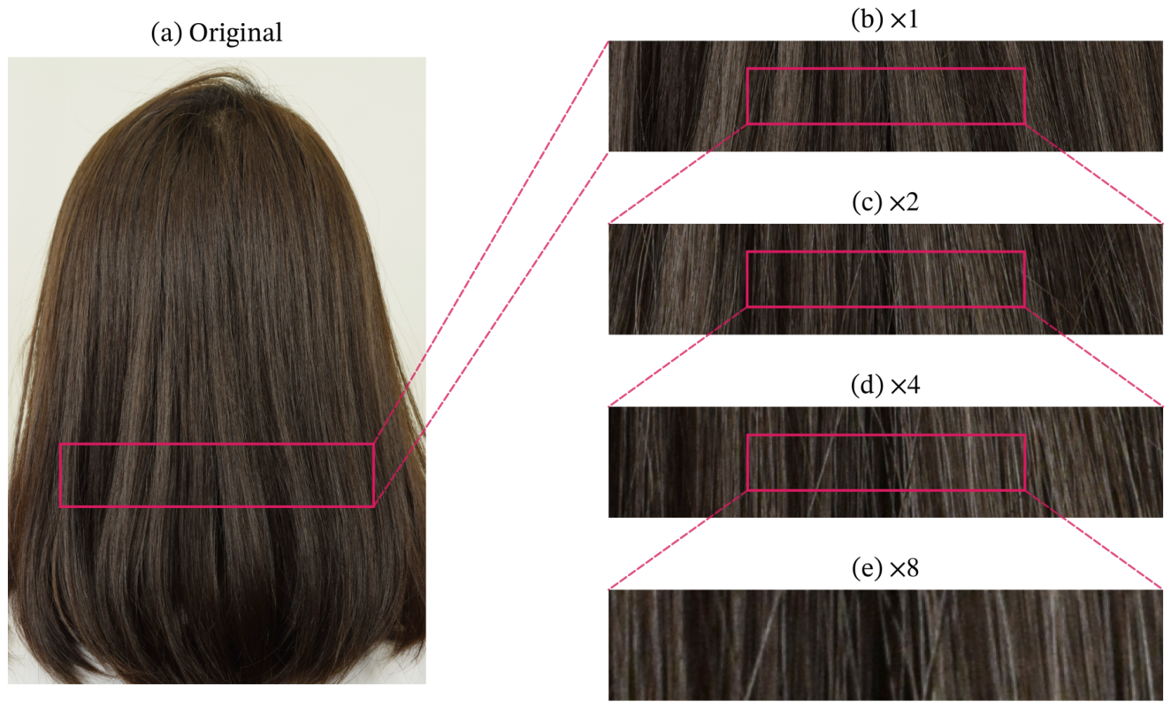
Figure 2.
Representative back-view hair photographs from the dataset. Twenty-four images were randomly selected from the 145 participants to illustrate the diversity of hair color, length, and texture.
Figure 2.
Representative back-view hair photographs from the dataset. Twenty-four images were randomly selected from the 145 participants to illustrate the diversity of hair color, length, and texture.
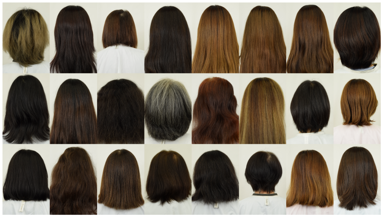
Figure 3.
Illustration of scale-dependent texture using fractional Gaussian noise signals (left) and grayscale images formed by repeating each signal vertically (right). The Hurst exponents are (a) , (b) , and (c) ; for this model, . All signals have zero mean and unit variance, but increasing the exponent changes the visual texture from fine alternating fluctuations to broader, more gradually varying features. The relationship between the exponent and spatial correlations is described in Appendix A.2.
Figure 3.
Illustration of scale-dependent texture using fractional Gaussian noise signals (left) and grayscale images formed by repeating each signal vertically (right). The Hurst exponents are (a) , (b) , and (c) ; for this model, . All signals have zero mean and unit variance, but increasing the exponent changes the visual texture from fine alternating fluctuations to broader, more gradually varying features. The relationship between the exponent and spatial correlations is described in Appendix A.2.
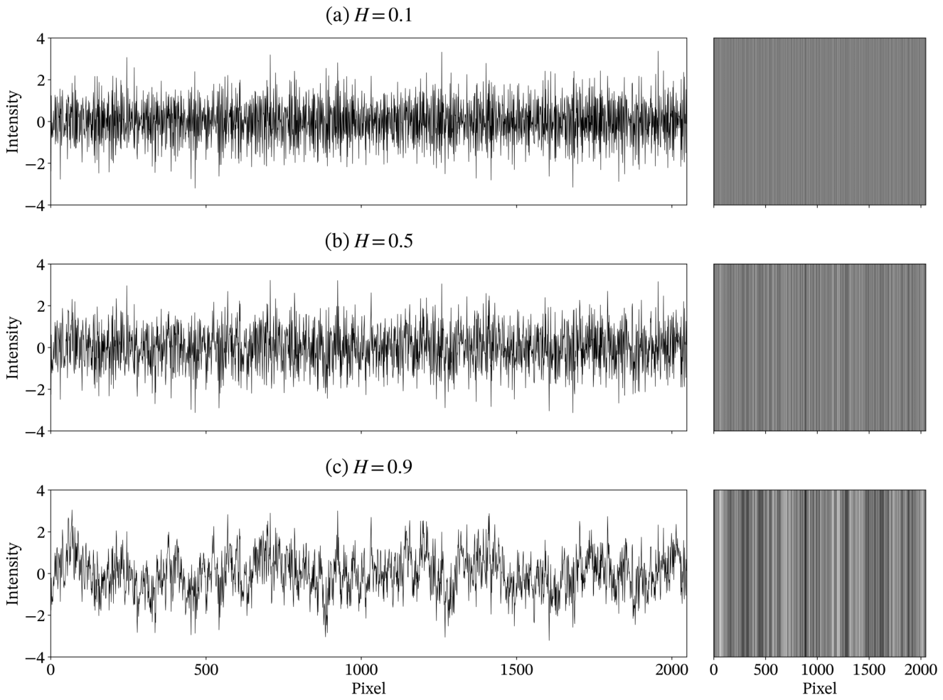
Figure 4.
Representative hair image, transverse intensity signals, and DMA results. (a) Full hair photograph with dashed lines marking the upper and lower signal-extraction rows. (b, d) Upper and lower intensity signals, respectively. (c, e) Corresponding fluctuation functions and linear fits for DMA(0) (red) and DMA(2) (blue). Numerical annotations in red and blue in these panels indicate quantities calculated using DMA(0) and DMA(2), respectively. The photograph is gamma-adjusted () for display only; signals and estimates use the original image intensities.
Figure 4.
Representative hair image, transverse intensity signals, and DMA results. (a) Full hair photograph with dashed lines marking the upper and lower signal-extraction rows. (b, d) Upper and lower intensity signals, respectively. (c, e) Corresponding fluctuation functions and linear fits for DMA(0) (red) and DMA(2) (blue). Numerical annotations in red and blue in these panels indicate quantities calculated using DMA(0) and DMA(2), respectively. The photograph is gamma-adjusted () for display only; signals and estimates use the original image intensities.
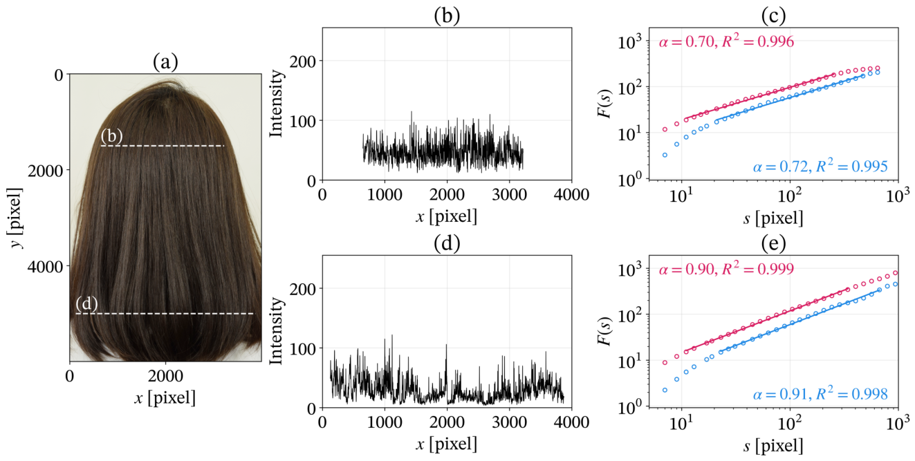
Figure 5.
Row-wise DMA results for the entire hair region of a representative participant. (a) Hair photograph, with the red outline indicating the analyzed hair region. (b) Vertical variation of the coefficient of determination for DMA(0) (red) and DMA(2) (blue). (c) Vertical variation of the estimated DMA exponent for DMA(0) (red) and DMA(2) (blue). The photograph is gamma-adjusted () for display only; all profiles are based on the original image intensities.
Figure 5.
Row-wise DMA results for the entire hair region of a representative participant. (a) Hair photograph, with the red outline indicating the analyzed hair region. (b) Vertical variation of the coefficient of determination for DMA(0) (red) and DMA(2) (blue). (c) Vertical variation of the estimated DMA exponent for DMA(0) (red) and DMA(2) (blue). The photograph is gamma-adjusted () for display only; all profiles are based on the original image intensities.
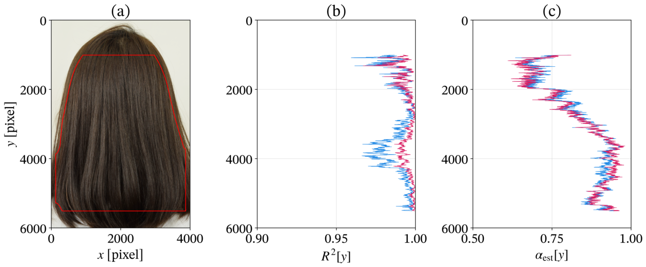
Figure 6.
Distributions of the coefficient of determination obtained using (a) DMA(0) and (b) DMA(2). For each participant, the filled marker indicates the median, and the vertical error bar spans the 5th to 95th percentiles of across the valid y-positions. Participants are shown in ascending order of the median obtained using DMA(0), with the same participant order retained for DMA(2). The large hollow marker and error bar to the left of each panel indicate the median and the 5th–95th percentile range, respectively, derived from the global ECDF obtained by equally averaging the participant-specific ECDFs. The vertical black line separates the global summary from the participant-specific results.
Figure 6.
Distributions of the coefficient of determination obtained using (a) DMA(0) and (b) DMA(2). For each participant, the filled marker indicates the median, and the vertical error bar spans the 5th to 95th percentiles of across the valid y-positions. Participants are shown in ascending order of the median obtained using DMA(0), with the same participant order retained for DMA(2). The large hollow marker and error bar to the left of each panel indicate the median and the 5th–95th percentile range, respectively, derived from the global ECDF obtained by equally averaging the participant-specific ECDFs. The vertical black line separates the global summary from the participant-specific results.
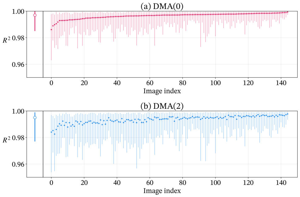
Figure 7.
Spatial variation in the estimated DMA exponent along the normalized vertical coordinate for (a) DMA(0) and (b) DMA(2). Thin lines show individual participant profiles, while thick lines represent the estimated population-level mean profiles with shaded pointwise 95% confidence intervals. The mean profiles and confidence intervals are displayed only at positions covered by the observed ranges of at least 50% of participants.
Figure 7.
Spatial variation in the estimated DMA exponent along the normalized vertical coordinate for (a) DMA(0) and (b) DMA(2). Thin lines show individual participant profiles, while thick lines represent the estimated population-level mean profiles with shaded pointwise 95% confidence intervals. The mean profiles and confidence intervals are displayed only at positions covered by the observed ranges of at least 50% of participants.
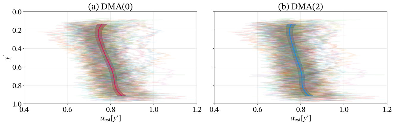
Figure 8.
Example of deviation from single power-law scaling. (a) Hair photograph with the selected row marked in white. (b) Extracted intensity signal. (c) Fluctuation functions for DMA(0) (red) and DMA(2) (blue), with single-exponent linear fits over the fitting ranges in Equation (2) (solid lines). The fitted exponents and coefficients of determination are shown in red for DMA(0) and blue for DMA(2) in panel (c). The photograph is gamma-adjusted () for display only; the signal and DMA results use the original image intensities.
Figure 8.
Example of deviation from single power-law scaling. (a) Hair photograph with the selected row marked in white. (b) Extracted intensity signal. (c) Fluctuation functions for DMA(0) (red) and DMA(2) (blue), with single-exponent linear fits over the fitting ranges in Equation (2) (solid lines). The fitted exponents and coefficients of determination are shown in red for DMA(0) and blue for DMA(2) in panel (c). The photograph is gamma-adjusted () for display only; the signal and DMA results use the original image intensities.
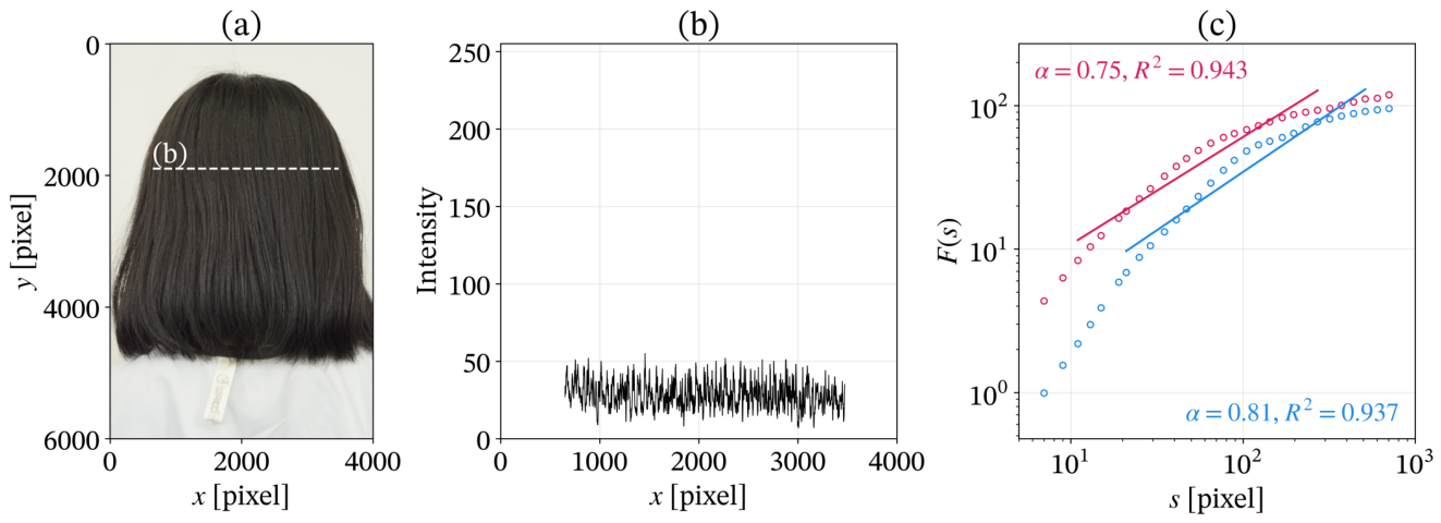
Figure 9.
Differences between the DMA exponents estimated using DMA(0), , and DMA(2), . Each black marker and error bar represents the mean and standard deviation of the differences across the valid y-positions for an individual participant. The white marker and error bar indicate the mean and standard deviation across all valid y-positions pooled across the dataset.
Figure 9.
Differences between the DMA exponents estimated using DMA(0), , and DMA(2), . Each black marker and error bar represents the mean and standard deviation of the differences across the valid y-positions for an individual participant. The white marker and error bar indicate the mean and standard deviation across all valid y-positions pooled across the dataset.
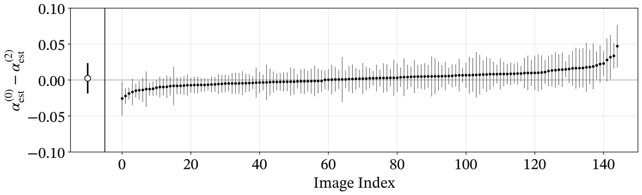
Figure 10.
Example with a large difference between DMA orders. (a) Hair photograph with the selected row marked in white. (b) Extracted intensity signal. (c) Fluctuation functions and linear fits for DMA(0) (red) and DMA(2) (blue). Numerical annotations in red and blue in panel (c) indicate quantities calculated using DMA(0) and DMA(2), respectively.
Figure 10.
Example with a large difference between DMA orders. (a) Hair photograph with the selected row marked in white. (b) Extracted intensity signal. (c) Fluctuation functions and linear fits for DMA(0) (red) and DMA(2) (blue). Numerical annotations in red and blue in panel (c) indicate quantities calculated using DMA(0) and DMA(2), respectively.
Disclaimer/Publisher’s Note: The statements, opinions and data contained in all publications are solely those of the individual author(s) and contributor(s) and not of MDPI and/or the editor(s). MDPI and/or the editor(s) disclaim responsibility for any injury to people or property resulting from any ideas, methods, instructions or products referred to in the content. |
© 2026 by the authors. Licensee MDPI, Basel, Switzerland. This article is an open access article distributed under the terms and conditions of the Creative Commons Attribution (CC BY) license.
Copyright: This open access article is published under a Creative Commons CC BY 4.0 license, which permit the free download, distribution, and reuse, provided that the author and preprint are cited in any reuse.