
Submitted:
17 November 2026
Posted:
18 November 2026
You are already at the latest version
Abstract
For binary linear codes with binary phase-shift keying over additive white Gaussian noise at high signal-to-noise ratio, most maximum-likelihood decoding errors involve codewords nearest the one sent. Their number equals that of minimum-weight codewords: nonzero codewords with the fewest ones. Reliability-based polar construction does not always minimize this number. This paper finds the minimum within a family of polar-transform codes of length N=2m. Each code retains all rows with N or N/2 ones and b≥1 rows with N/4 ones, zeroing other inputs, giving minimum distance N/4. For m≥5 and 1≤b≤m, the minimum is 4max{b,3b−m}, with all optimal selections identified. At length 64 with 16 information bits, it is 152, versus a published construction’s 196. On binary-input memoryless symmetric channels, polar codes chosen by exact reliability, with ties respecting the decreasing order, must select certain rows together, so, in this family, they cannot attain the minimum for m≥5 and 2≤b≤m. At lengths 32, 64 and 128, polar codes in this family built for an erasure channel with erasure probability 0.5 have up to 3.29 times the minimum, by exhaustive enumeration.
Keywords:
polar codes
; polar transform
; information-position selection
; minimum-weight codewords
; quadratic forms
; Reed–Muller subcodes
1. Introduction
Arıkan introduced polar codes as an efficient construction that achieves the capacity of symmetric binary-input memoryless channels as the code length grows [1]. In practical systems, including the control channels of 5G New Radio [2], polar codes operate at finite lengths. At these lengths, code design must consider both the reliability of individual information inputs and the distances between complete codewords [3].
The minimum distance measures the fewest bit positions in which two distinct codewords differ. The weight of a binary word is its number of ones. For a binary linear code, the nonzero codewords with the fewest ones are its minimum-weight codewords, and their weight equals the minimum distance. Codes with the same minimum distance can still have different numbers of minimum-weight codewords. This number is called the minimum-weight count. For a linear code, it also equals the number of other codewords at the minimum distance from any transmitted codeword. Reliability-based construction does not directly minimize it. Rowshan, Dau and Viterbo modify polar information positions to reduce the count while accounting for any loss in the reliability of the selected inputs [3]. The exact minimum provides a benchmark for comparing row selections at the same code length, number of information bits and minimum distance. This paper determines such minima when every row of the polar-transform matrix with weight N or is retained and a prescribed number of rows of weight is selected, where N is the code length.
Consider a length-16 polar code carrying seven information bits and having minimum distance four. Table 1 compares this code with a second code obtained by replacing one information position. A synthetic channel describes how the received signal and the known earlier input bits provide information about one encoder input. For a binary erasure channel with erasure probability , Code A uses the seven inputs with the smallest exact synthetic-channel erasure probabilities. Code B replaces information position 10 with position 3, reducing the number of minimum-weight codewords from twelve to eight while preserving the code length, number of information bits and minimum distance. Row and input indices start at zero. No bit-reversal permutation is applied: the binary digits of each index are not reversed (Section 2). Section 2.2 derives both counts.
For a binary linear code with minimum distance d, let denote the minimum-weight count, that is, the number of codewords with exactly d ones. For binary phase-shift keying over additive white Gaussian noise, the union bound gives an upper bound on maximum-likelihood decoding error probability. At high signal-to-noise ratio, its largest contribution comes from minimum-weight codewords and is proportional to . Reducing at fixed distance, rate and channel conditions reduces this contribution, but does not guarantee a gain for a particular decoder. A decoder’s performance also depends on the reliability of the selected inputs [3,4].
The count can be studied by writing each row as a polynomial. A monomial is a product of distinct variables. For length , each polar-transform row is obtained by listing a monomial’s values for all binary assignments to the m variables [4,5]. The constant gives a row of weight N, a single variable (a linear monomial) gives weight , and a product of two distinct variables (a quadratic monomial) gives weight . In polynomial form, the studied family retains the constant and every linear monomial, and selects exactly quadratic monomials. The same polynomial description turns row selection into a graph problem. Each variable is represented by a vertex, and an edge between vertices i and j represents the selected product .
The optimization changes only which rows are selected. Every selected input carries an independent bit and every other input is fixed to zero. This restriction excludes polar subcodes with dynamic frozen bits: encoder inputs whose values are fixed by binary linear combinations of other inputs [6]. The code rate is the number of information bits divided by the code length, here . It is at most in Theorem 1 and equals in the length-64 case of Theorem 2.
At length 64, retaining the row of weight 64 and all six rows of weight 32, then choosing nine rows of weight 16, gives 16 information bits and minimum distance 16. Changing the nine weight-16 rows can therefore change the minimum-weight count without changing these parameters. The polar code constructed for erasure probability with 16 information bits belongs to this family. Section 5 compares its count with the smallest possible count and examines further polar codes at lengths 32 and 128.
Reed–Muller codes use the same transform but select rows by weight rather than by reliability. The degree of a monomial is the number of variables it contains. The Reed–Muller code of order r retains every monomial of degree at most r, or equivalently every row of weight at least . The first-order code therefore keeps the constant and all linear monomials, and the second-order code also keeps every quadratic monomial. Choosing the number of quadratic rows also provides numbers of information bits between those of the two Reed–Muller codes at a fixed length, a motivation also considered by Vaideeswaran, Harish and Natarajan [7]. Each code in the studied family contains the first-order code and is contained in the second-order code. The second-order Reed–Muller code has no nonzero codeword with fewer than ones, so neither does a code contained in it. Each studied code also contains a selected quadratic row with exactly ones. Its minimum distance is therefore exactly , as explained in Section 2. The classical description of minimum-weight codewords in the second-order Reed–Muller code [8,9] can therefore be used to identify those retained by each selection. Keeping the constant and every linear term allows these codewords to be counted exactly.
The method for counting minimum-weight codewords in this family is already known. Tokushige, Takata and Kasami studied a broader family, which includes these codes as second-order Reed–Muller codes with selected quadratic monomials removed. Their optimization theorem covers a range with few removed monomials [10,11]. The description of minimum-weight codewords by Rowshan, Dau and Viterbo also shows when the count equals its lower bound [3]. Each selected quadratic monomial, together with the retained constant and linear terms, gives four minimum-weight codewords. With b selected quadratic monomials, the count is exactly when no two share a variable. Their graph edges are then disjoint, meaning that they have no vertex in common. This requires distinct variables. Thus forces the count above , but does not give the smallest attainable count.
Selecting rows by channel reliability adds an ordering restriction. Polar codes built from exact channel reliabilities under the conditions in Section 5 make decreasing selections: selecting a monomial requires certain others to be selected too [5]. Rowshan and Drăgoi minimize the minimum-weight count within the decreasing quadratic family and use a specified reliability order to distinguish selections with equal count [4]. More recently, Rowshan and Drăgoi combine reliability and minimum-weight counts in a single cost, and they also optimize it only over decreasing selections [12]. The optimization here allows arbitrary quadratic selections and minimizes the count alone.
The contributions are as follows.
- Theorem 1 gives the minimum for and , and identifies every selection that reaches it. For , disjoint selected edges are impossible, and the new minimum is . For example, with four selected quadratic monomials in six variables, the smallest minimum-weight count is 24, although the simple lower bound gives only 16.
- Theorem 2 gives the minimum 152 for six variables and nine selected quadratic monomials, attained by a triangular prism. The published block construction has count 196 [7]. The smaller count of 152 shows that the block construction is not optimal in general, contrary to the belief stated in Remark 2 of [7].
- Corollary 1 shows that no decreasing selection attains the minimum of Theorem 1 when and . For six variables and nine selected quadratic monomials, the smallest minimum-weight count among decreasing selections is 300. The erasure-channel polar code at erasure probability has count 364, compared with the minimum of 152 over all selections. Section 5 specifies the selected quadratic pairs and calculates the count.
- For every possible number of selected quadratic rows at lengths 32, 64 and 128, exact enumeration determines the smallest minimum-weight count. Table 2 compares these minima with every polar code in this family constructed for erasure probability at those lengths. With two or more quadratic rows, these polar codes have between approximately and times the smallest count.
The counting formula in Lemma 1 and the formula for decreasing codes are established results. It is also known that the count equals exactly when the selected edges are disjoint. The new results are the minimum counts and the selections that reach them in the parameter ranges identified above.
2. From Polar-Transform Rows to Quadratic Monomials
Let be an integer and the code length. Use the polar-transform matrix
The notation means the Kronecker product of m copies of F. Let denote row i of , with indices starting at zero. No bit-reversal permutation is applied.
A code in this family retains every row of weight N or and selects b of the rows of weight , where . Each retained row is assigned an independent information bit, while all remaining encoder inputs are frozen to zero. The encoder then forms the codeword by taking the exclusive-OR (XOR) of the retained rows whose information bits are one.
To count the minimum-weight codewords, use the polynomial description of these rows. Let be binary variables and write , where the superscript denotes transpose. All polynomial coefficients and matrix operations are over , so addition is XOR. Multiplication is ordinary multiplication of binary values. In particular, . Number output positions by , and write using all m binary digits, including leading zeros. Thus is the least significant bit. Set at position c. For one variable, evaluating gives and evaluating the constant 1 gives , the two rows of F. The Kronecker product extends this correspondence to m variables [4,5].
If S is the set of variable indices in a monomial, evaluating that monomial at all output positions gives row , where
The set S is empty for the constant 1, which gives row . For example, at length 16 the product has , so its row index is .
The retained rows are therefore the evaluations of the constant, all m linear monomials and b distinct quadratic monomials. Let B contain the selected pairs of variable indices, so means is retained and is the number of selected pairs. Each information bit is the coefficient of one retained monomial, while the variables describe output positions. Let denote the resulting code. Its length N, dimension K and minimum distance d are
The retained rows are linearly independent, so the K information bits generate distinct codewords. The full second-order Reed–Muller code, denoted , retains every quadratic as well as the constant and every linear monomial. It has minimum distance [8]. The subcode cannot have a smaller distance. It contains a selected quadratic row with exactly ones, so its minimum distance is also . Let denote the minimum-weight count of .
At length 16, the row for equals one at positions 0, 4, 8 and 12, where . Retaining the constant and every linear term also allows the four products
Each product equals one for a different pair of values of , while the other two variables can take either binary value. It therefore gives four ones. For example, represents the XOR of rows 12 and 13. These are four minimum-weight codewords with the same quadratic part, meaning the same sum of degree-two terms. The graph description below identifies the additional quadratic parts that can arise when selected products share variables.
2.1. Counting Codewords from the Selected Edges
Represent the selection by a graph G with vertices . An edge means that is retained. There are no loops or repeated edges, so G is a simple graph. Two vertices are neighbors when an edge joins them, and a path is a sequence of distinct vertices in which each consecutive pair are neighbors. The degree of vertex v is the number of edges meeting that vertex, or equivalently the number of selected products containing .
A codeword can use some or all of the selected quadratic monomials. For its quadratic part, , form the symmetric matrix Q with and zero diagonal. Such a matrix is called alternating over . Its rank is the number of linearly independent rows. The support graph of Q has edge precisely when . It is contained in G because an unselected monomial cannot have a nonzero coefficient.
The next lemma identifies two types of support graph that give minimum-weight codewords. A complete bipartite graph divides its vertices into two nonempty groups and contains every edge between the groups, with no edge within a group. A complete tripartite graph has the same property with three nonempty groups. Let count the distinct edge sets contained in G that form one of these two types of graph. The subscript 2 refers to the rank of the quadratic coefficient matrix. Each such edge set is called a support. It gives four minimum-weight codewords, as proved in Lemma 1 below. Vertices that meet no edge in the support are ignored. A support need not include every available edge between its vertices. Edges left out have coefficient zero. For example, a triangle contains three different two-edge paths as well as the triangle itself. Together with its three single edges, these give seven counted supports.
Lemma 1
(Established counting facts in graph form). For the code in (1),
Proof.
An affine factor is a binary linear combination of the variables plus a constant. For example, is an affine factor, where addition is XOR. The selected rows lie in the second-order Reed–Muller code. The classical description of its minimum-weight codewords expresses a weight- word as the evaluation of a product of two affine factors with independent linear parts [8]. If are independent, the four products are
The product equals one when and . These two independent binary equations leave free binary choices, giving positions. The four choices of give four distinct sets of positions. When the product is expanded, terms containing become linear because for binary variables. All four have the same quadratic coefficient matrix , of rank two. Conversely, every rank-two alternating matrix has this form. Its column space is the span of u and v. Choosing a different basis for this same space gives the same four sets of positions in a different order. Thus each such quadratic part gives exactly four minimum-weight codewords.
To identify the support graph, group its vertices i according to . The three possible nonzero pairs are , and . The entry is one exactly when vertices i and j have different nonzero pairs. Vertices with pair meet no edge in the support. Since u and v are independent, two or three of the nonzero pairs occur. The support is therefore complete bipartite or complete tripartite, as stated in [13]. Conversely, assigning different nonzero pairs to the groups produces every support of either type. A support determines Q uniquely. All lower-degree monomials are retained, so each of the four codewords with that quadratic part, formed by adding constant and linear terms, belongs to . □
With at least three variables, a triangle illustrates the complete tripartite supports in Lemma 1. The triangle on vertices gives the four products , with . For , the expansion is . The three quadratic terms give the triangle, and the linear term is available because every linear monomial is retained.
2.2. Counting the Length-16 Example
To count the minimum-weight codewords of Code A in Table 1, first identify the rows selected using exact channel reliabilities. For a binary erasure channel, let z be the erasure probability at one step of the polar recursion. The next two values are and [1]. Starting from , read all four binary digits of an input index from most significant to least significant, including leading zeros. Use the first update for a zero and the second for a one. The seven smallest resulting erasure probabilities occur at indices , giving Code A. For example, index 10 has binary digits 1010 and gives
In Table 1, both codes retain rows , corresponding to . Code A also retains rows 12 and 10, corresponding to and . Its graph has two edges meeting at vertex 1. The counted supports are the two single edges and the two-edge path formed by taking both edges. Each support gives four minimum-weight codewords, so Lemma 1 gives . The twelve words are the evaluations of the three families
where . Each family has four words. No codeword belongs to two families because their quadratic parts differ. For , the last product is , which evaluates to . Here ⊕ denotes XOR. It has four ones, so this row combination supplies a minimum-weight codeword in addition to those arising from either quadratic alone.
Code B replaces row 10 by row 3, replacing by . Its graph has two disjoint edges. Only the two single edges are complete bipartite or tripartite supports, giving . Their codewords come from and . The same erasure recursion gives about for input 3, compared with for input 10. Thus the replacement reduces the minimum-weight count while selecting a less reliable synthetic channel. Choosing by reliability and choosing to reduce the count therefore give different codes, even at length 16.
3. The Exact Minimum for at Most m Selected Quadratic Monomials
The graph count can also identify which row choices minimize the number of minimum-weight codewords. The next theorem describes these choices using paths and cycles. A cycle joins distinct vertices in sequence and closes the sequence by joining the last vertex to the first. Its length is its number of edges. The components of a graph are its separate connected pieces. The construction for uses a cycle through all m vertices. The restriction prevents that cycle from being a triangle or a four-cycle, either of which would contribute a counted support in addition to its edges and two-edge paths.
Theorem 1
(Exact minimum for at most m selected quadratic monomials). Let and . Among all codes retaining and exactly b quadratic monomials, the smallest minimum-weight count is
If , a selection attains this minimum exactly when its edges are disjoint. Unused vertices are allowed. If , a selection attains this minimum exactly when every vertex has degree one or two and the graph has no triangle or four-cycle. Equivalently, its components are paths with at least one edge and cycles of length at least five, covering all m vertices. When , every component must be a cycle of length at least five.
Proof.
Every edge contributes one support counted by . Every choice of two neighbors of vertex v gives a two-edge path, which is another complete bipartite support. Its centre is unique, so no path is counted twice. There are such choices at vertex v. Consequently,
For the second inequality, the path count is nonnegative, for every nonnegative integer k, and because each edge has two endpoints.
If , equality requires . Equation (5) then forces every degree to be at most one, so the selected edges must be disjoint. Conversely, b disjoint edges exist in this range, and their only counted supports are the edges themselves.
The difference is zero exactly when or . Thus every vertex must have degree one or two. With these degrees, a complete bipartite support can only be an edge, a two-edge path or a four-cycle. A complete tripartite support can only be a triangle. Thus the edges and two-edge paths are the only supports exactly when the graph has no triangles or four-cycles. These conditions are both necessary and sufficient for . A graph with every degree one or two consists of paths with at least one edge and cycles. Excluding triangles and four-cycles ensures that every remaining cycle has length at least five. When , the average degree is two, so every component is a cycle.
Selections meeting these conditions exist for every b in this range. For , select disjoint edges and one path on vertices. These components use all m vertices and exactly b edges. There are two-edge paths, one centred at each internal vertex of the longer path. Hence .
Finally, if , select a cycle through all m vertices. Since , it contains no triangle or four-cycle. Again, its only counted supports are its m edges and m two-edge paths. Thus . Multiplying these counts by four proves (4). □
For , the same bound and constructions give exact counts 4, 8 and 20 for , respectively. A single edge, two disjoint edges and a four-vertex path attain them. This includes Code B in Table 1.
To illustrate the minimum when disjoint edges are no longer possible, take and . Equation (1) gives length , dimension and minimum distance , written . Select
The graph consists of two three-vertex paths. It has four edges and two two-edge paths, giving . Equation (5) shows that no other four-monomial selection has a smaller count. The four quadratic rows have indices . Including the constant and all six linear rows gives information positions
All other inputs are frozen to zero.
4. The Exact Minimum for Nine Quadratic Monomials at Length 64
The previous theorem covers selections with no more quadratic monomials than variables. The next comparison uses and . It lies outside Theorem 1, so a separate optimality proof is needed. Every selection has parameters . Vaideeswaran, Harish and Natarajan consider a construction that, for two blocks of three variables, deletes the quadratic monomials within each block [7]. This is blocks of size in their notation, giving six variables in the notation used here. With blocks and , the retained graph is , the complete bipartite graph with three vertices in each group. Every counted support is obtained by choosing a nonempty subset from each group. There are seven choices per group, so
Instead, retain the six edges of the triangles and , together with the joining edges , and . This graph, denoted , is a triangular prism. Let denote its monomial selection. The six omitted edges form the cycle . Figure 1 shows both retained graphs.
Table 3 lists every type of counted support in . A star has one centre joined to one or more leaves, with no other edge included in its support. The prism has degree three at every vertex, giving two-edge paths and six three-edge stars. Each pair of the three edges joining the triangles determines one four-cycle, giving three four-cycles. There are two triangles.
No larger support is missing from the table. Degree three excludes stars with more than three leaves. Any pair of prism vertices has at most two common neighbors. This excludes complete bipartite supports with at least two vertices in one group and at least three in the other. Also, adjacent prism vertices have at most one common neighbor. A complete tripartite support larger than a triangle would contain two adjacent vertices with two common neighbors, so none occurs. Lemma 1 therefore gives
The prism therefore gives fewer minimum-weight codewords than the block construction. The comparison shows, contrary to the belief in Remark 2 of [7], that the block construction is not optimal for two blocks of three variables. The count of 196 proved for that construction is unaffected. It remains to show that no other selection has a smaller count.
Theorem 2
(Length-64 optimum). Among all codes retaining and exactly nine quadratic monomials, the minimum value of is 152. The prism selection attains this value.
Proof.
Let G be any graph on six vertices with nine edges. Its degrees satisfy . For each vertex v, every nonempty subset of its neighbors gives a star support. There are such subsets. Summing over all vertices counts each single edge twice. Every star with at least two edges has a unique centre and is counted once. Subtracting the nine repeated counts gives
First suppose that the degrees are not all three. Since their average is three, some degree is at least four and another is at most two. To bound the sum in (9), compare the six degree values while keeping their total equal to 18. Replacing a pair with , where and , preserves the sum of the degrees and decreases by . Repeating this step makes all six degrees equal to three. At least one step was required, so
Equation (9) therefore shows that G contains at least 37 star supports.
The graph must also contain a triangle or a four-cycle. If no triangle occurs, the endpoints of every two-edge path are nonadjacent. If two distinct two-edge paths had the same endpoints, their different centres would form a four-cycle. A graph containing neither type of cycle could therefore have at most one two-edge path for each of its nonadjacent vertex pairs. However, the degree sum and the inequality used in (5) give
This contradiction shows that G must contain a triangle or a four-cycle. A triangle is a complete tripartite support and a four-cycle is a complete bipartite support. Neither is a star, so at least one additional support occurs. Thus when the degrees are not all three.
Now suppose that every vertex has degree three. The complement of G, formed from its omitted edges, has degree two at every vertex. A finite simple graph of degree two is a union of cycles, each with at least three vertices. With six vertices, the complement is therefore either one six-cycle or two disjoint triangles. After renumbering the variables if needed, the retained graph is a triangular prism or . Changing the variable numbers does not change the number of counted supports, so their counts are 38 and 49, respectively, as established above. Every possible G therefore satisfies . The prism attains 38, and (2) gives the minimum . □
5. Polar Codes and Decreasing Selections
The minima in Theorems 1 and 2 are taken over all choices of quadratic rows. Comparing these minima with polar codes also requires the rule governing which information positions must be selected together. Use the variable order in [4], but start the indices at 1: the variable called there is called here. A quadratic selection is decreasing when selecting with requires every with , and to be selected too. For example, selecting requires as well. Here, reliability is measured by the Bhattacharyya parameter, a measure of similarity between the channel-output distributions for the two input-bit values. Smaller values are preferred. For an erasure channel, it equals the erasure probability used in Section 2.2. For binary-input memoryless symmetric channels, selecting inputs by their exact Bhattacharyya parameters gives a decreasing set when ties are resolved consistently with this order [5].
The comparison uses the minimum-weight counting formula for decreasing monomial codes given by Bardet et al. [5]. Rowshan and Drăgoi review it in their Equation (7) and give complete weight distributions for the decreasing quadratic family in Theorem 6 [4]. The next result compares the smallest count under the decreasing restriction with the smallest count over all allowed row selections.
Corollary 1
(Decreasing selections cannot reach the minimum). For and , no decreasing selection B attains the minimum in Theorem 1. For and , the exact minimum over decreasing selections is 300, whereas Theorem 2 gives 152 without the decreasing restriction.
Proof.
Let t be the largest vertex index used by a selected edge. The decreasing rule forces the edges for every . Thus vertex 1 is adjacent to every other used vertex. If , then , so the selected edges cannot be disjoint. A decreasing selection therefore cannot attain the minimum for . For , any selection attaining the minimum in Theorem 1 must use every vertex and have every degree at most two. Then , so vertex 1 has degree , a contradiction.
For a decreasing quadratic selection, the established counting formula [4], with variable indices starting at 1 as in this paper, is
In (12), each selected pair contributes a fixed positive amount. For six variables, the nine smallest factors are . They correspond to
This selection is decreasing, so the lower bound obtained by taking the nine smallest contributions is attained. Its count is
Thus 300 is the smallest count among decreasing selections, and it exceeds the minimum of 152 over all selections. □
No polar information set in this family that follows the decreasing order can reach the minimum count in the ranges stated in Corollary 1. The corollary says nothing about information sets outside this family.
For Code A, Equation (12) gives for the selected pairs and . Section 2.2 obtained the same count as , from two single-edge supports and one two-edge path. The two formulas group the same codewords differently.
The erasure channel provides a concrete comparison between reliability selection and these minima. Applying the erasure-channel recursion of Section 2.2 with six-bit indices, including leading zeros, and erasure probability gives polar codes in this family for . At , the selected quadratic pairs are those of with replaced by . All channel erasure probabilities are different, so no tie needs to be broken when selecting the inputs. Equation (12) gives
Thus exact reliability selection gives 364 weight-16 codewords, compared with 300 for the best decreasing selection and 152 without the decreasing restriction. All three codes have parameters .
The same comparison can be made at lengths 32, 64 and 128 for all polar codes constructed for erasure probability that belong to this family. These codes have 7–14, 8–17 and 12–21 information bits, respectively. For each length, all quadratic-row selections were enumerated using Python 3.12.14 with NumPy 2.3.5. For each selection, the rank-two supports contained in its graph were counted. Four times this number is the minimum-weight count, by Lemma 1. This determines the minimum for every , including cases outside Theorems 1 and 2. As an independent check, all codewords were enumerated for one minimizing selection at each b with , and for every polar code in Table 2 with . All counts agreed. The enumeration script, complete results and verification records are available from the author on request.
Table 2 reports the cases corresponding to these polar codes. With two or more quadratic rows, their minimum-weight counts are between approximately and times the smallest count at the same length, dimension and minimum distance. These are count comparisons, not measured decoding gains.
Theorem 1 applies to a smaller proportion of the polar codes in this family at the longer lengths checked. For erasure probability at length 256, it covers only the code with in this family. At lengths 512 and 1024, every polar code in the family constructed for the same erasure probability selects more than m quadratic rows, so neither theorem applies. These checks do not establish the same statement for other channels or all larger lengths.
6. Relationship to Earlier Results
The earlier work addresses two different problems: counting the minimum-weight codewords for a given row selection, and finding the selection with the smallest count. Tokushige, Takata and Kasami considered subcodes obtained by deleting monomials of the highest retained degree while keeping every lower-degree monomial [10]. Chapter 2 of Tokushige’s thesis gives a determinant test for deciding which minimum-weight codewords remain in the subcode, an inclusion–exclusion count that corrects for codewords counted more than once, and an optimization theorem for the deleted monomials [11]. For quadratic selections, let be the number of deleted monomials. That theorem states that, when , the count is smallest exactly when the deleted monomials have no variables in common. Throughout the range of Theorem 1,
For the six-variable case in Theorem 2, , so . Theorems 1 and 2 therefore concern cases that Tokushige’s optimization theorem does not cover. His counting method still applies to these selections. One enumerated case in Table 2 does fall within that optimization range. For , two quadratic monomials are omitted, and the minimum 204 agrees with Tokushige’s theorem [11].
The results used to count the minimum-weight codewords for a fixed selection of quadratic rows are also established. Classical second-order Reed–Muller theory relates codeword weights to the rank of the quadratic coefficient matrix [8] [9]. With every constant and linear term available, each rank-two quadratic part gives four minimum-weight codewords. Hora’s Lemma 3.8 identifies the corresponding graph as complete bipartite or complete tripartite [13]. Lemma 1 expresses this count using the selected edges, so different row choices can be compared directly.
Van Wonterghem, Boutros and Moeneclaey used the positions where two transform rows both contain a one to guide selection [14]. Rowshan, Dau and Viterbo describe how minimum-weight codewords are formed from transform rows [3]. Applying their description to the second-order Reed–Muller code, and keeping only the codewords built from selected rows, shows when the count equals its simple lower bound . The disjoint-edge condition stated in the Introduction also follows directly from Lemma 1. Theorem 1 determines the smallest count and every selection that attains it for and , where disjoint edges are impossible.
The comparisons above assume that each selected transform row carries its own independent information bit. Allowing one information bit to control a combination of rows changes the problem. For , using the constant, every linear monomial and the single generator gives dimension and minimum distance , by classical quadratic-form theory [8]. The coefficient of this combined generator is one bit shared by two transform rows, so it does not select those inputs independently. Linking rows in this way is allowed in polar subcodes with dynamic frozen bits [6]. It produces different codes, possibly with a larger minimum distance, so it falls outside the row-choice problem studied here.
7. Conclusions
Polar codes choose their information positions by channel reliability, but this choice need not minimize the number of minimum-weight codewords. This paper finds the smallest possible count, in the parameter ranges below, for one family of polar-transform codes of length , where m is the number of binary variables. These codes retain every row of weight N or , select b rows of weight and freeze all other inputs to zero.
For and , the smallest count is . Theorem 1 also identifies every row choice that reaches this count. When , the selected quadratic monomials must share no variables. When , every variable must be used, and each connected component of the selected graph must be a path with at least one edge or a cycle with at least five edges. For six variables and nine selected quadratic rows, the minimum is 152, attained by the triangular prism. This is lower than the published block construction’s count of 196.
The decreasing order used in polar construction requires certain monomials to be selected together. Polar codes built from exact channel reliabilities follow this order, under the channel conditions and the rule for equal reliabilities given in Section 5. For and , no decreasing selection reaches the minimum. For six variables and nine quadratic rows, the best decreasing selection has 300 minimum-weight codewords, while the polar code for an erasure channel with erasure probability has 364, compared with the minimum of 152. At lengths 32, 64 and 128, polar codes in this family constructed for erasure probability with two or more quadratic rows have between approximately and times the smallest count (Table 2). A code’s minimum-weight count can therefore be compared with the smallest possible count at the same length, number of information bits and minimum distance, whether its information positions were chosen by reliability or by minimum-weight count.
For more than m selected quadratic rows, Theorem 2 determines the minimum for . Tokushige’s optimization theorem applies when twice the number of omitted quadratic rows does not exceed m (Section 6). For every possible number of selected quadratic rows at lengths 32, 64 and 128, exact enumeration determines the smallest minimum-weight count. Table 2 reports the cases corresponding to polar codes constructed for erasure probability . The minima for the polar-code parameters identified at lengths 512 and 1024 for that erasure probability are not determined here.
All these count comparisons assume that each selected row carries an independent information bit. Codes that link rows through dynamic frozen bits can behave differently. Even within the studied family, fewer minimum-weight codewords alone do not guarantee better performance with a particular decoder.
Author Contributions
The author is the sole contributor to this work.
Funding
No funding was received for this study.
Institutional Review Board Statement
Not applicable.
Informed Consent Statement
Not applicable.
Data Availability Statement
The proofs are included in this article. The enumeration script, complete results and verification records used for Table 2 are available from the author on request.
Acknowledgments
OpenAI ChatGPT (GPT-6 Astra) and Anthropic Claude (Opus 5.5) assisted with checking mathematical arguments, the enumeration code and LaTeX preparation. The author takes full responsibility for the final manuscript.
Conflicts of Interest
The author declares no conflicts of interest.
References
- Arıkan, E. Channel Polarization: A Method for Constructing Capacity-Achieving Codes for Symmetric Binary-Input Memoryless Channels. IEEE Trans. Inf. Theory 2009, 55, 3051–3073. [Google Scholar] [CrossRef]
- GPP. 5G; NR; Multiplexing and Channel Coding. Technical Specification TS 38.212, ETSI, 2025. Version 18.6.0, Release 18; ETSI TS 138 212 V18.6.0.
- Rowshan, M.; Dau, S.H.; Viterbo, E. On the Formation of Min-Weight Codewords of Polar/PAC Codes and Its Applications. IEEE Trans. Inf. Theory 2023, 69, 7627–7649. [Google Scholar] [CrossRef]
- Rowshan, M.; Drăgoi, V.F. Weight Structure of Low/High-Rate Polar Codes and Weight Contribution-Based Partial Order. IEEE Trans. Inf. Theory 2025, 71, 9340–9358. [Google Scholar] [CrossRef]
- Bardet, M.; Drăgoi, V.; Otmani, A.; Tillich, J.P. Algebraic Properties of Polar Codes From a New Polynomial Formalism. In Proceedings of the 2016 IEEE International Symposium on Information Theory (ISIT), Extended version; July 2016; pp. 230–234. [Google Scholar] [CrossRef]
- Trifonov, P.; Miloslavskaya, V. Polar Subcodes. IEEE J. Sel. Areas Commun. 2016, 34, 254–266. [Google Scholar] [CrossRef]
- Vaideeswaran, A.P.; Harish, M.S.; Natarajan, L.P. Subcodes of Second-Order Reed–Muller Codes via Recursive Subproducts. In Proceedings of the 2025 IEEE International Symposium on Information Theory (ISIT), June 2025; pp. 1–6. [Google Scholar] [CrossRef]
- MacWilliams, F.J.; Sloane, N.J.A. The Theory of Error-Correcting Codes; North-Holland: Amsterdam, The Netherlands, 1977. [Google Scholar]
- Sloane, N.J.A.; Berlekamp, E.R. Weight Enumerator for Second-Order Reed–Muller Codes. IEEE Trans. Inf. Theory 1970, 16, 745–751. [Google Scholar] [CrossRef]
- Tokushige, H.; Takata, T.; Kasami, T. On the Number of Minimum Weight Codewords of Subcodes of Reed–Muller Codes. IEICE Trans. Fundam. Electron. Commun. Comput. Sci. 1998, E81-A, 1990–1997. [Google Scholar]
- Tokushige, H. Soft-Decision Decoding Algorithms for Binary Linear Block Codes. NAIST-IS-DT9861014; Doctoral thesis. Nara Institute of Science and Technology, 2000. [Google Scholar]
- Rowshan, M.; Drăgoi, V.F. A Hybrid Reliability–Weight Framework for Construction of Polar Codes. 2026. Available online: https://arxiv.org/abs/2601.10376v2.
- Hora, J. Steiner Forms. Comment. Math. Univ. Carol. 2016, 57, 527–536. [Google Scholar] [CrossRef]
- Van Wonterghem, J.; Boutros, J.J.; Moeneclaey, M. On Constructions of Reed–Muller Subcodes. IEEE Commun. Lett. 2018, 22, 220–223. [Google Scholar] [CrossRef]
Figure 1.
Retained quadratic monomials for two codes. Each edge represents . Both codes also retain the constant and all six linear monomials. Line crossings without a numbered circle are not vertices.
Figure 1.
Retained quadratic monomials for two codes. Each edge represents . Both codes also retain the constant and all six linear monomials. Line crossings without a numbered circle are not vertices.
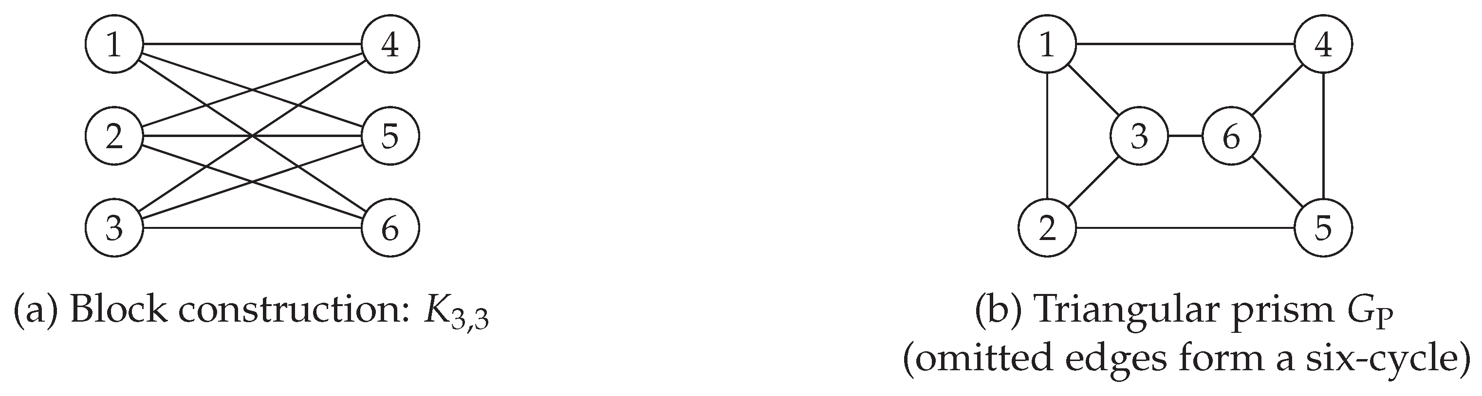

Table 1.
Two length-16 polar-transform selections carrying seven information bits. Both have minimum distance four and 128 codewords. Code A uses exact erasure-channel reliability at erasure probability . All unlisted inputs are frozen to zero.
Table 1.
Two length-16 polar-transform selections carrying seven information bits. Both have minimum distance four and 128 codewords. Code A uses exact erasure-channel reliability at erasure probability . All unlisted inputs are frozen to zero.
| Code | Information positions | Minimum-weight codewords |
|---|---|---|
| A | 12 | |
| B | 8 |
Table 2.
Smallest minimum-weight count over all selections of b quadratic rows and the count for the polar code chosen by exact erasure-channel reliability at erasure probability . Every such polar code in the studied family at lengths 32, 64 and 128 is included. The ratio is the polar count divided by the smallest count, rounded to two decimal places. The final column identifies the theorem or enumeration that establishes the minimum.
Table 2.
Smallest minimum-weight count over all selections of b quadratic rows and the count for the polar code chosen by exact erasure-channel reliability at erasure probability . Every such polar code in the studied family at lengths 32, 64 and 128 is included. The ratio is the polar count divided by the smallest count, rounded to two decimal places. The final column identifies the theorem or enumeration that establishes the minimum.
| N | K | b | Smallest count | Polar count | Ratio | Basis |
|---|---|---|---|---|---|---|
| 32 | 7 | 1 | 4 | 4 | 1.00 | Thm. 1 |
| 8 | 2 | 8 | 12 | 1.50 | Thm. 1 | |
| 9 | 3 | 16 | 28 | 1.75 | Thm. 1 | |
| 10 | 4 | 28 | 44 | 1.57 | Thm. 1 | |
| 11 | 5 | 40 | 76 | 1.90 | Thm. 1 | |
| 12 | 6 | 76 | 108 | 1.42 | Enumeration | |
| 13 | 7 | 124 | 172 | 1.39 | Enumeration | |
| 14 | 8 | 204 | 236 | 1.16 | Enumeration | |
| 64 | 8 | 1 | 4 | 4 | 1.00 | Thm. 1 |
| 9 | 2 | 8 | 12 | 1.50 | Thm. 1 | |
| 10 | 3 | 12 | 28 | 2.33 | Thm. 1 | |
| 11 | 4 | 24 | 44 | 1.83 | Thm. 1 | |
| 12 | 5 | 36 | 76 | 2.11 | Thm. 1 | |
| 13 | 6 | 48 | 140 | 2.92 | Thm. 1 | |
| 14 | 7 | 80 | 172 | 2.15 | Enumeration | |
| 15 | 8 | 116 | 236 | 2.03 | Enumeration | |
| 16 | 9 | 152 | 364 | 2.39 | Thm. 2 | |
| 17 | 10 | 252 | 428 | 1.70 | Enumeration | |
| 128 | 12 | 4 | 20 | 44 | 2.20 | Thm. 1 |
| 13 | 5 | 32 | 76 | 2.38 | Thm. 1 | |
| 14 | 6 | 44 | 140 | 3.18 | Thm. 1 | |
| 15 | 7 | 56 | 172 | 3.07 | Thm. 1 | |
| 16 | 8 | 84 | 236 | 2.81 | Enumeration | |
| 17 | 9 | 116 | 364 | 3.14 | Enumeration | |
| 18 | 10 | 152 | 428 | 2.82 | Enumeration | |
| 19 | 11 | 208 | 684 | 3.29 | Enumeration | |
| 20 | 12 | 296 | 812 | 2.74 | Enumeration | |
| 21 | 13 | 396 | 1068 | 2.70 | Enumeration |
Table 3.
Complete bipartite and tripartite supports contained in the retained prism graph . Each support contributes four weight-16 codewords.
Table 3.
Complete bipartite and tripartite supports contained in the retained prism graph . Each support contributes four weight-16 codewords.
| Support | Number of supports | Weight-16 codewords |
|---|---|---|
| Single edge | 9 | 36 |
| Two-edge path | 18 | 72 |
| Three-edge star | 6 | 24 |
| Four-cycle | 3 | 12 |
| Triangle | 2 | 8 |
| Total | 38 | 152 |
Disclaimer/Publisher’s Note: The statements, opinions and data contained in all publications are solely those of the individual author(s) and contributor(s) and not of MDPI and/or the editor(s). MDPI and/or the editor(s) disclaim responsibility for any injury to people or property resulting from any ideas, methods, instructions or products referred to in the content. |
© 2026 by the authors. Licensee MDPI, Basel, Switzerland. This article is an open access article distributed under the terms and conditions of the Creative Commons Attribution (CC BY) license (http://creativecommons.org/licenses/by/4.0/).
Copyright: This open access article is published under a Creative Commons CC BY 4.0 license, which permit the free download, distribution, and reuse, provided that the author and preprint are cited in any reuse.