
Submitted:
16 November 2026
Posted:
18 November 2026
You are already at the latest version
Abstract
Distributed maritime sensing requires receive-beamforming and power-allocation decisions based on short interference-training records and subject to limited cooperative-link capacity. We formulate a design that maximizes the worst-node signal-to-interference-plus-noise ratio (SINR) with a squared 2-Wasserstein ambiguity set and a radius explicitly selected using an engineering rule. A homogeneous worst-case quadratic form yields a complete second-order cone programming (SOCP) formulation at a fixed SINR threshold. A loaded receive update is distinguished from this exact block, and both are followed by power allocation using the complete robust denominator. A power iteration with upward quantization and a mean-preserving quantized tracker provide hard-budget feasibility checks on a reliable shared broadcast channel. We derive coupled error bounds and a conditional bound on the gap to a centralized power optimum computed using the same data and fixed receive weights; joint stationarity is not established. In 200 paired simulations with known ensemble clutter covariance and a spatial jamming surrogate, certified loading achieves mean worst-node SINRs of 2.663 and 1.928 dB when evaluated using the true covariance and the robust denominator, respectively. Both certified loading and the exact-receive branch have zero observed robust violations, whereas the reduced-denominator diagnostic violates the complete constraint in every trial. A 256-bit round cap is enforced before sending, and small per-round messages do not imply lower traffic over a complete coherent processing interval (CPI): certified loading uses a mean of 20.799 kbit over the 200 core scenes, compared with 20.802 kbit for a matched centralized implementation with one binary64 Hermitian covariance upload, the same three redesign rounds, and a final return. This matched comparison demonstrates no complete-CPI traffic advantage. Independent detector counts, paired confidence intervals, solver statuses, and per-trial feasibility records are released.
Keywords:
distributed sensing network
; joint receive beamforming and power allocation
; Wasserstein distributionally robust optimization
; limited interference snapshots
; limited-backhaul communication
; consensus optimization
1. Introduction
1.1. Research Background
Distributed sensing networks exploit spatial diversity by coordinating separated nodes. In a maritime setting, receive beamforming and transmit power depend on short interference records, changing propagation, and finite cooperative-link capacity. Limited samples can distort sample-covariance beamformers; cooperative algorithms can also incur substantial traffic even when each message is small. These limitations motivate a joint formulation with explicit information and communication accounting.
1.2. State of the Art and Limitations
Distributed resource allocation, robust beamforming, and communication-aware optimization provide relevant foundations. The present study examines their interaction in a specified monostatic network with fixed transmit codes and geometry-based mutual interference. It does not assume that all earlier methods require full covariance exchange. The central question is whether local robust receive updates and scalar power coordination can produce verifiable feasible outputs, and how much communication this requires over a full interval.
1.3. Key Challenges
The three technical questions are: how to represent the complete robust SINR constraint at a fixed threshold; how to distinguish a loaded approximation from the exact receive block; and how power quantization, budget tracking, and coordination messages affect feasibility and the comparison with a power reference computed using the same data.
1.4. Contributions
The contribution is a fully specified and reproducible combination of robust receive design and quantized power coordination. It relies on established Wasserstein, diagonal-loading, and interference-mapping ideas; its claims are limited to the reformulation, conditional error analysis, and reported simulation evidence.
(1) We formulate joint receive-beamforming design and power allocation with fixed constant-modulus transmit codes, local sample covariances, known calibration covariances, and explicit power limits. The transmit codes are not optimization variables.
(2) We derive the complete homogeneous worst-case quadratic form and fixed-threshold SOCP. We separately specify a loaded receive approximation and a conservative constant-modulus SDP surrogate. The radius is an engineering rule without a distribution-free coverage claim.
(3) We specify a reliable shared-broadcast protocol, quantize both transmitted scalar variables, preserve the tracker mean, and derive a coupled error bound. Full-CPI accounting includes control messages and compressed covariance uploads and return transmissions in the centralized scheme.
(4) We release paired comparisons of exact and loaded receive updates, independent robust residuals, solver and power-trial ledgers, detector counts and uncertainty estimates, and parameter sweeps. Ideal exact block updates imply only a monotone bounded objective-value sequence; no joint stationary-point or approximate stationary-neighborhood guarantee is asserted.
1.5. Organization of the Paper
Section 2 reviews related work and identifies the differences from the closest prior work; Section 3 establishes the system model and the joint optimization problem; Section 4 and Section 5 present, respectively, the distributionally robust receive-beamforming design and distributed power allocation with low per-round communication; Section 6 presents the alternating implementation, convergence results, runtime accounting, and reproducibility records; Section 7 reports the simulation experiments; Section 8 discusses the limitations; and Section 9 concludes the paper. The main symbols are listed in the symbol table at the end of Section 3, and the proofs of the propositions and theorems are given in the appendices.
2. Related Work
2.1. Distributed/Networked Sensing Resource Allocation
Radar-network coordination is surveyed in [1], while sea-clutter properties and anti-jamming interactions are reviewed in [2,3]. Distributed-aperture waveform construction is studied in [4]. Decentralized radar resource allocation [5] and decomposition methods [6] provide optimization precedents. Network-level ISAC and trajectory/resource allocation [7,8] involve related but distinct system assumptions. These works motivate the current setting; their communication costs and performance cannot be inferred from generic algorithm names alone.
2.2. Robust and Distributionally Robust Waveform/Beamforming Design
Practical waveform and receive-filter design is studied in [9,10], and ISAC beamforming in [11,12]. These application labels do not identify a common uncertainty set. Moment uncertainty [13] differs from empirical Wasserstein uncertainty [14]. Irani et al. [15] constrain distributions of the interference covariance and desired steering vector through support, mean/similarity, and moment information. Wang et al. [16] study local/global distributional robustness, regularization, and Bayesian nonparametric constructions for snapshot or interference-plus-noise covariance uncertainty. These methods must not all be classified as Wasserstein-ball designs. Our additional scope is coupled power control with fixed transmit codes and an executable broadcast protocol.
2.3. Low-Communication Distributed Optimization
ADMM provides a general distributed-optimization framework [17,18], but its generic convergence theory does not determine the communication cost of a specific radar implementation. Distributed-aperture waveform shaping [19], repeater-jamming transceiver design [20], and cooperative radar-communication waveform design [21] address complementary problems. Their published algorithms provide context; the controlled comparisons in this study do not implement these algorithms in full.
2.4. Differences from the Closest Prior Work
Table 1 distinguishes the design objects of representative studies. Table 2 separately identifies their uncertainty models. Neither table is a numerical ranking of complete published algorithms.
Table 1 separates the objects of the cited work from the scope of this implementation. Communication advantages must be evaluated for a fully specified protocol and refresh schedule.
2.5. In-Depth Comparison with Existing DRO and Distributed Optimization Methods
The relevant distinctions are the uncertainty set, the information supplied to design, and the communication protocol. General Wasserstein DRO [14], moment-based beamforming [15], the broader constructions in [16], and application-specific ADMM must be compared on these separate terms.
Wasserstein DRO can model uncertainty around an empirical distribution [14]. Its statistical guarantees depend on the support, tails, dimension, and radius construction. Our noise-anchored radius is an engineering specification; covariance estimation stability alone does not establish Wasserstein coverage.
Distributed ADMM and related methods [6,17,18] exchange application-dependent primal, dual, or consensus information. We do not assign them a universal covariance-sized message. The current power problem has a scalar local decision, but all interfering powers must be available; the numerical deployment therefore assumes broadcast reception by all nodes.
Scalar power coupling is enabled by fixed codes, calibrated geometry, and receive-side processing that does not depend on a neighbor’s receive vector. The implemented protocol broadcasts two scalar payloads plus separately counted controls. It is restricted to reliable shared broadcast; extension to sparse graphs requires routing, aggregation, and new analysis. Because all powers are heard, the tracker is not necessary for exact sum-budget checking in this deployment.
Relative to classical robust Capon and diagonal-loading designs [22,23], the present model places an empirical squared-Wasserstein ambiguity set on the external interference snapshots while keeping target steering and calibration known. The exact worst-case denominator contains a norm-product cross term that the loaded inverse update omits. The power iteration is an instance of the established interference-mapping approach [24,25], rather than a new power-control principle. Our incremental contribution is the combination of complete-denominator certification, a fixed-threshold receive SOCP, an executable quantized broadcast procedure with hard power and message limits, and conditional finite-resolution error bounds under the stated fixed-code model. The released matched comparisons assess this combination; they do not establish general superiority over the underlying classical methods.
Accordingly, a dedicated methodological comparison is given in Table 2.
The comparison in Table 2 defines scope rather than a ranking of algorithms. Section 7 reports only controlled variants whose complete implementation is released.
Further relevant work includes antenna placement and power allocation [26], small sea-target detection [27], measured clutter Doppler characteristics [28], geometric covariance estimation [29], and likelihood-based robustness [30]. Communication-efficient learning and distributed nonconvex methods are developed in [31,32,33,34,35]. ISAC opportunities, limits, and hybrid beamforming are discussed in [36,37,38,39]. These references provide context; equivalence to their full methods is not claimed.
3. System Model and Problem Formulation
3.1. Network Topology and Cooperative Link Model
Consider a distributed network comprising M spatially separated sensing nodes, whose set is denoted . Node m transmits a fixed constant-modulus waveform cm of code length N (with the pointwise constant-modulus constraint ), and its discrete baseband transmit signal is
Here pm is the transmit power and cm is the fixed unit-energy constant-modulus code, with coherent processing gain G = N. The adaptive receive vector wm acts across antenna elements. The numerical cooperative network is a reliable synchronous shared broadcast channel: each node hears all transmitted powers. Sparse-graph and packet-loss extensions are outside the implemented protocol.
Assumption 1 (monostatic operation and calibrated coupling). Each node receives its own target echo. All nodes share a frequency band and use fixed preallocated transmit codes. Code cross-correlations and node-to-node directions are stored calibration inputs. Mutual interference depends on local wm, known geometry, and the broadcast powers, but not on a neighbor’s receive-weight vector. Multistatic illumination would require a separately specified target and information model.
Assumption 2 (CPI and calibration). Geometry and target gain are fixed within each coherent processing interval (CPI); known local target gain, ensemble clutter covariance, and noise level are calibration inputs. The power-coupling matrix changes when the local receive weights change, even if geometry is fixed. Geometry may be refreshed between CPIs;Section 7 tests stale and refreshed directions. Detector frames assume slow texture shared by their pulses and reference cells.
Assumption 3 (communication accounting). Each complete protocol round includes all transmissions in its ordered phases, rather than one scalar transmission. The main configuration sets Cmax = 256 bit per round; the network-size sweep explicitly uses Cmax = 64M bit. The simulator checks the accumulated round payload before every send and raises an error before an excess frame is emitted. A normal inner round sends two q-bit scalars and two control bits per node. Opening thresholds, closing decisions, and final selection/certificate reports are also counted. This is a payload constraint under reliable synchronous broadcast; packet headers, coding, acknowledgments, and physical airtime are outside the model.
Figure 1 distinguishes outer receive/power updates, threshold trials, inner messages, and held-out evaluation.
Each of three outer rounds updates local receive weights and then runs quantized power coordination. The feasible round with the highest accepted threshold is retained, with the latest round selected on an exact tie. Selection uses this public threshold, rather than held-out SINR or a later certificate report. Every outer round contributes to timing and traffic; there is no global early-stopping test.
3.2. Signal, Sea-Clutter, and Active-Jamming Models
Each node is equipped with a uniform linear array (ULA) of na antenna elements (with element spacing d = λ/2); the transmit waveform has code length N and a coherent pulse-compression processing gain G = N. Adaptive anti-jamming is performed along the antenna-element (spatial) dimension, and the receive beamforming weight vector is denoted . Let u = sinθ denote the spatial direction cosine; then the array steering vector in direction u is
The target lies in the antenna boresight direction (ut = 0), and its matched steering vector is . Sidelobe-directed barrage jamming and dense false targets impinge from the direction set (). Two types of mismatch are considered: first, due to platform motion and jammer maneuvering, the true interference directions drift by a small angle Δu relative to the training directions, so that the training covariance and the true covariance differ; second, a small amount of target-echo energy leaks into the training snapshots (the signal-preservation problem), and with few samples, direct matrix inversion can suppress the target as if it were interference. Each node can estimate the interference covariance only from the most recent L element snapshots; when L is of the same order as na or smaller (L≲2na), this constitutes the data-scarcity regime, which is the main operating regime addressed by the distributionally robust design.
The baseband echo vector received by node m is denoted
In (3), β is the co-channel isolation amplitude and β² is its power factor, set to 0.01. The radius parameter is ζ, a separate symbol. Sea clutter has a compound-Gaussian representation [40] with unit-mean texture, so its ensemble covariance equals the stated Rc.
The texture has shape ν and scale 1/ν, hence Eτ = 1. Rc is the ensemble clutter covariance as well as the speckle covariance under this normalization. Conditional on the texture, the clutter vector is circular complex Gaussian with covariance τRc; the speckle vector is independent of the texture and has covariance Rc. Active interference is modeled through a spatial Gaussian covariance surrogate; this is not a full time-domain DRFM simulator. Noise has covariance σn²I. The simulation supplies Rc as a known calibration input.
Node m has L available training vectors. Their sample second moment is formed as follows; the simulation explicitly adds target contamination to the training data, so this is the covariance of the available vectors rather than an oracle interference covariance.
When the effective number of snapshots L is of the same order as the array dimension na and the available samples are insufficient, exhibits a significant mismatch relative to the true RJ,m; designing receive beamformers directly from it leads to performance degradation. Section 4 characterizes this uncertainty using a Wasserstein distributionally robust formulation.
3.3. Signal-to-Interference-plus-Noise Ratio and Detection Model
After fixed-code pulse compression and application of the receive weight wm, the per-pulse ensemble output SINR is
where W = [w1,…,wM], p = [p1,…,pM]^T, and ; G = N is the coherent processing gain associated with the code length, and a(0) is the steering vector in the target boresight direction. The first term in the denominator represents external interference, sea clutter, and thermal noise; at design time only the sample covariance and its Wasserstein-robust correction are available, while the true covariance is used solely for evaluation, and the difference between the sample and true covariances reflects the mismatch caused by limited data. The second term represents co-channel mutual interference from the other nodes’ fixed codes; after matched filtering it is given by , where the link isolation factor β2 corresponds to about −20 dB (set to β2 = 0.01), χmk is the stored code cross-correlation coefficient, and a(umk) is the known direction vector of the interference from node k. Because it depends only on the local weight and the stored deployment parameters, the mutual-interference term is evaluated without exchanging any receive-weight vector. Mutual-interference components are modeled as mutually uncorrelated zero-mean returns, so their covariance contributions add without cross-node coherent terms. This second-order assumption is also used in the detector simulation.
Equation (6) defines per-pulse ensemble SINR. For independent complex-Gaussian pulses with known total variance and deterministic equal target magnitude, the normalized energy sum has 2np degrees of freedom and noncentrality 2npSINR. The following ideal known-variance curve is a model prediction. It is not the exact detection probability of a finite-reference-window CFAR detector in compound-Gaussian clutter. Here F denotes the cumulative distribution function and the overbar denotes its complementary distribution function; the inverse inside the argument is the central chi-square quantile.
We set np = 6 and Pfa = 10⁻⁴. Section 7 separately validates a detector using 32 independent reference cells conditional on a shared texture, four excluded guard cells, independent H0 threshold calibration, and held-out H0/H1 observations. Its uncertainty is computed from detection counts; the ideal curve is not substituted for those counts.
3.4. Joint Optimization under Sample and Communication Constraints
Sample scarcity means only L local training vectors are available, with no evaluation covariance supplied to the optimizer. For communication, payload and control bits both contribute to the implemented budget. The general per-round accounting is
Here nm(t) counts scalar payloads and cctrl(t) includes every flag and decision in that complete round. The executable constraint uses Cmax = 256 bit in the main study and Cmax = 64M bit in the explicitly identified scaling study. Section 5 specifies the send order and checks. We maximize the worst-node robust SINR using the complete denominator in Section 4.
The transmit code is fixed and already obeys the pointwise constant-modulus constraint cm ( already implies ∥cm∥2 = 1, so the energy constraint is not repeated); the spatial receive beamforming weight wm has unit energy ∥wm∥2 = 1. Introducing an auxiliary variable γ, the max–min problem is equivalent to
Lemma 1 (nonconvex structure). The joint problem couples powers and local receive weights through quadratic interference terms and the SINR threshold. A unit-energy representative is convenient for interpretation but does not itself define a convex set. Optional constant-modulus receive constraints introduce an additional nonconvex restriction. The transmit code is fixed and adds no decision-variable nonconvexity.
For fixed positive p and γ, an alternative unit-target-response normalization gives a convex receive SOCP (Proposition 2). With fixed W and γ, power feasibility is linear (Proposition 4). These separate properties do not imply joint convexity. The optional constant-modulus SDP is a separately defined conservative relaxation (Proposition 3).
3.5. Main Notation
Table 3 lists the main notation. The following conventions are used throughout: bold uppercase W = [w1,…,wM] denotes the collection of beamforming weights (a matrix), while lowercase wm is the beamforming vector of node m; bold lowercase p = (p1,…,pM)T is the transmit power vector, and uppercase P is reserved for the power bounds Pmax,Ptot, the probability Pr, and the detection/false-alarm probabilities Pd,Pfa; the transmit code is denoted cm and the covariance by R.
4. Distributionally Robust Receive Beamforming
4.1. Ambiguity Set and Engineering Radius
Each node forms an empirical distribution from its local interference snapshots. The radius ε is the radius in squared 2-Wasserstein distance, not W₂ itself. The clutter covariance Rc and thermal-noise power are treated as known calibration inputs; estimating these quantities jointly from short contaminated training windows is outside the present model. The training sample covariance may include the explicitly simulated target contamination, so the ambiguity set is centered on the distribution of the available training vectors rather than on an unobservable interference-only population.
Proposition 1 (radius specification). We use the following nonnegative engineering rule. It specifies a design parameter and does not establish a probability that the true distribution belongs to the ambiguity set. In particular, a covariance concentration inequality does not imply a Wasserstein coverage inequality. C = 2.5 and ζ = 0.05 are fixed before the evaluation runs; the radius sweep is a sensitivity analysis, not tuning on the test seeds. The value C=2.5 is an empirical design setting retained from the earlier implementation. No independent optimization study or geometry-specific calibration is claimed for this numerical choice.
The radius has units of power and decreases with the number of snapshots. Changing the interference distribution, calibration covariance, or training contamination requires a new calibration study. The framework of [14] motivates ambiguity-set modeling, while [29] addresses distributionally robust covariance estimation; neither supplies a coverage theorem for the particular rule (14).
4.2. Exact Worst-Case Quadratic Form
Lemma 2. On unrestricted complex Euclidean support, with squared Euclidean transport cost and a finite empirical second moment, the worst-case quadratic form is the following homogeneous expression. No unit-norm assumption is needed.
For a = ‖w‖² > 0 and c = wᴴR̂w > 0, the scalar dual and its minimizer are given below. When c = 0 or ε = 0 the same value follows by continuity, although the infimum need not be attained at an interior dual multiplier. Appendix A gives a direct coupling proof, including these boundary cases.
4.3. Complete Fixed-Threshold SOCP
For fixed positive powers, define Qm as the sum of known clutter, thermal noise, and mutual interference. All its terms are positive semidefinite and independent of wm. The robust SINR uses the complete denominator.
Proposition 2. Fix γ > 0 and pm > 0. For any feasible weight with nonzero target response, homogeneity and a phase rotation allow a(0)ᴴwm = 1. The full constraint Γm ≥ γ is then equivalent to the following SOCP feasibility system. A matrix square root B satisfies BᴴB = R; the Hermitian positive-semidefinite square root is used in the implementation.
The complex target-response equality is imposed on its real and imaginary parts. The two nonnegative auxiliary variables in (18) separately bound the covariance norm and the radius norm; their sum is bounded by tm. Each norm epigraph is a second-order cone, and the final cone has a constant right-hand side when powers and threshold are fixed. Eliminating the two auxiliary bounds recovers the sum-of-norms inequality. Minimizing an epigraph z for the final norm gives the exact local receive optimum in (19), without threshold bisection. Unit-energy normalization is applied only afterwards; it preserves the homogeneous ratio and is not imposed simultaneously with unit target response.
4.4. Loaded Approximation and Optional Constant-Modulus Branch
The inexpensive receive-weight update replaces φε by wᴴR̂w + ε‖w‖². This removes the nonnegative cross term in (15), so the loaded update is a surrogate and is not the exact SOCP solution. Classical diagonal loading provides related motivation [22,23,41]; the fixed 20% shrinkage comparator in Section 7 is not presented as a fitted Ledoit–Wolf estimator.
The implemented loaded method subsequently uses the exact expression (15) in the power block and in the final constraint check. Thus its beam update is approximate, but its returned SINR certificate is checked against the exact robust denominator. A separate loaded-surrogate diagnostic uses the reduced denominator in the power block to quantify the failure caused by treating loading as an exact robust reformulation. It is not the deployed method.
Proposition 3 (conservative constant-modulus relaxation). If receive hardware additionally requires |wi| = 1/√na, use Young’s inequality with a fixed ηY > 0: φε(w) ≤ (1 + ηY)wᴴR̂w + (1 + 1/ηY)ε‖w‖². Let AηY = (1 + ηY)R̂ + Q + (1 + 1/ηY)εI. Lifting X = wwᴴ and dropping the rank-one constraint gives a relaxation of this conservative surrogate, not of the exact robust objective. With fixed p, the Charnes–Cooper variables Y = X/tr(AηYX) and z = 1/tr(AηYX) give the SDP below.
maxY,z|αm|2pmGtr(a(0)a(0)HY)
The SDP value upper-bounds the optimum of the conservative constant-modulus surrogate only. It is not a global upper bound on the original exact-Wasserstein constant-modulus optimum. A rank-one X = Y/z yields the conservative optimum; otherwise Gaussian randomization produces feasible constant-modulus vectors. All candidate scores include noise exactly once. We use ηY = 1 and nested candidate sets to compare 200, 500, 1000, 2000, and 4000 draws. Related constant-modulus optimization methods are discussed in [9,10,42,43]. Equation (21) maximizes the conservative ratio at fixed powers without introducing a SINR threshold; it is a separate surrogate optimization rather than the exact constant-modulus counterpart of (18). The symbol Y≽0 denotes Hermitian positive semidefiniteness.
5. Quantized Power Coordination and Error Bounds
5.1. Fixed-Weight Power Feasibility
For fixed W, define am = |αm|²G|a(0)ᴴwm|², bmk = Gβ²|χmk|²|wmᴴa(umk)|² with bmm = 0, and dm = φεm(wm) + wmᴴ(Rc,m + σn²I)wm. Nodes with zero target gain cannot meet a positive threshold. For positive gains, let Fmk = bmk/am and vm = dm/am. Only local sample information and stored geometry enter each row; evaluation covariances never enter this construction.
Proposition 4. For fixed W and γ, these are linear inequalities. With v strictly positive, γρ(F) < 1 yields the componentwise smallest feasible fixed point p*(γ). A positive feasible solution cannot exist if γρ(F) ≥ 1. The power caps and total budget must still be checked.
Proposition 5. The exact feasible thresholds form an interval starting at zero; bisection and a linear-system solve provide a centralized reference for this fixed-W problem. It is not an upper bound on the complete joint W,p problem. The distributed implementation uses the common noise-only upper limit γU = maxm |αm|²G Pmax/σn², since the target steering vector has unit norm. This common physical bound is preconfigured; no global eigenvalue of F is requested by the algorithm. Standard interference mappings and related power-control formulations are discussed in [24,25].
5.2. Broadcast Protocol and Hard Feasibility Checks
The network is reliable synchronous shared broadcast with preconfigured node order and a designated threshold announcer; one transmission is heard by every node. The mixing matrix is J = 11ᵀ/M. At each threshold trial, the announcer sends the actual IEEE binary32 midpoint and all nodes use that decoded value. States reset to p = h = 0. In every inner round, each node first broadcasts a precheck flag for an out-of-range/nonfinite requested power or tracker state. Any failed precheck closes the trial with rejection before scalar transmission. Otherwise, each node broadcasts its upward-rounded power index on [0,Pmax] and nearest-grid tracker index on [−H,H], H = 4MPmax. The tracker itself remains local floating-point state. No sparse routing, loss, or asynchronous guarantee is claimed.
After all power/tracker payloads are decoded, nodes update (25). Each node then broadcasts a certification flag: its power has stabilized, its own complete SINR row passes tolerance, and the public node and total power budgets pass. Every node can compute the total directly from all decoded powers; the tracker is redundant for this sum check. The announcer accepts only when all certification flags are true. A budget failure, stable residual failure, saturation, or 200-round timeout closes the trial with a one-bit rejection; otherwise the next inner round begins. The decision is sent after the relevant flags. A normal completed round costs 2qM+2M bits, plus an opening 32-bit threshold and/or a closing one-bit decision where applicable. At M=4,q=16 the prescribed maximum is 169 bit, below Cmax=256 bit. Both the maximum-round requirement and every actual cumulative send are checked.
The accepted power vector is saved before trying a new threshold. Rejection supplies no certificate and does not prove continuous infeasibility; bisection therefore produces a conservative implementable threshold. Quantization never enlarges Pmax or Ptot. After three outer rounds, all nodes identify the largest accepted threshold, breaking ties in favor of the latest round. A final round sends its 32-bit threshold and two-bit index, followed by 32-bit downward-rounded local certificates (162 bit at M=4). Reports confirm the already selected output and do not determine retention. Nodes retain their own selected weight and the common selected powers. The ledger counts all trials and final traffic, including rejected attempts.
The round cap limits logical payload and control bits, rather than total CPI traffic or measured radio delay. It is slack in the main configuration: the observed maximum is 169 bit versus Cmax=256 bit. The released capacity checks reject Cmax=168 before the prescribed power protocol begins; Cmax=169 completes with the same returned design as Cmax=256. These checks establish compatibility with this phase grouping, not a minimum capacity for every possible protocol. In the scaling study Cmax=64M, the observed maximum at M=32 is 1121 bit against 2048 bit. Thus the measured utilization falls from 66.0% at M=4 to 54.7% at M=32. No physical latency guarantee follows without a link-rate, access, processing and retransmission model.
Here Sm = ampm and Dwc is recomputed directly from (15), known clutter/noise, and the final mutual-interference powers. A trial violates the robust constraints if any relative residual exceeds 10⁻⁶. Separate residuals check maxm(pm−Pmax,0) and max(Σpm−Ptot,0). The same checks apply to exact and loaded outputs. A log ratio between two denominator-based SINRs is not substituted for these residuals.
5.3. Coupled Power and Tracker Errors
Theorem 1. Consider a fixed threshold γ, fixed F and v, and no saturation. Without quantization, γρ(F) < 1 gives linear convergence of the power iteration. The tracker is a driven system, so its rate cannot be asserted to depend on the consensus eigenvalue alone. For the explicit quantized bounds below, assume the sufficient condition r = γ‖F‖∞ < 1 and a symmetric doubly stochastic Wc with λ = ‖Wc−J‖₂ < 1. The spectral-radius condition is weaker; when r ≥ 1 the displayed infinity-norm bound is not asserted, although a suitable weighted norm may still yield a contraction.
Unlike direct quantization of hnew, the increment-form tracker in (25) preserves the mean exactly for a doubly stochastic mixing matrix. Let zt = (I−J)ht. Then its recursion and a finite-time coupled bound are:
1Tht = 1Tpt
Equations (29)–(33) explicitly include power-driven tracking and both quantizers. Without quantization, the convolution gives a rate governed by max(r,λ), with a factor t when the rates coincide. Once the quantized power is stationary, the increment term vanishes, leaving only the tracker quantization floor. A pure λᵗ tracking-rate claim or exact convergence at finite q is therefore unwarranted. The reliable broadcast implementation has λ = 0. Graph-dependent extensions require their own routing and loss accounting [34,35,44,45,46,47,48,49].
5.4. Scope of the Power Gap and Communication Comparison
Define gW(p) as the minimum SINR with the same fixed W, sample covariance, radius, and known calibration terms. Over the box defined by the physical power limits, its infinity-norm Lipschitz constant can be bounded using vmin = minm vm > 0.
For a fixed threshold γ ≤ γW* with p*(γ) feasible, and an iterate pT that also passes the physical budget checks, the following conditional bound separates threshold backoff from communication error. Since gW(p*(γ)) = γ, it follows directly from the Lipschitz inequality. A rejected quantized threshold does not provide a continuous upper bound, so the first term must not be replaced by the binary-search interval width without an additional infeasibility proof.
Equation (36) uses the continuous power optimum at the returned fixed W and the identical training covariance, radius, and calibration. It bounds the actual gap γW* − gW(pT), rather than γW* minus the accepted threshold. The separate threshold-backoff term remains explicit. Table 9b reports the accepted threshold, achieved SINR, fixed-W reference, actual gap, and bound. This reference neither measures beam approximation/sampling error nor represents a joint global optimum. The matched centralized alternating baselines in Table 6 and Table 12 are separate comparisons.
For the matched centralized implementation, each node uploads its Hermitian sample covariance once using d² independent binary64 real values. The decoded covariance is bitwise identical to that used by broadcast design; known geometry, codes, clutter, noise, and radius are common calibration inputs. Both implementations execute three receive/power redesign rounds on these same samples. The centralized power block uses 42 continuous linear-system bisections. It returns the selected complex weights and powers as binary64 values, one binary64 threshold, and the selected outer index. At M=4,d=8 this costs 64M(d²+2d+1)+64+2 = 20802 bit. Payloads are divided into rounds of at most Cmax bits and checked before sending. An uncompressed complex covariance would cost 37186 bit with the same return. Covariance refresh count is one for both architectures; reusing the same covariance in three redesign rounds does not require three uploads. This transport simulation counts payloads, without modeling radio headers, acknowledgments, losses, or measured airtime.
6. Alternating Implementation and Reproducibility
6.1. Algorithm and Information Boundary
Algorithm 1 (receive-weight update). Form the local sample covariance once from the stored training vectors. Construct Qm from known clutter/noise and the currently broadcast powers. Solve (19) for the exact branch, or use (20) for the loaded branch. Normalize the returned vector to unit energy. CLARABEL is attempted first, followed by SCS; if both fail, the loaded fallback is explicitly logged. No evaluation covariance or unknown target perturbation is supplied to this function. For the optional constant-modulus surrogate, phase recovery uses default Nrand=1000 Gaussian candidates; nested 200, 500, 1000, 2000 and 4000 candidate sets test this empirical choice in Section 7.8.
Algorithm 2 (power update). Form each local row using the complete robust denominator for the loaded and SOCP branches. Run 20 binary32 threshold trials on the preconfigured physical upper bound. For each trial reset p,h, then execute the ordered precheck → scalar payload → certification-flag phases specified in Section 5.2 for at most 200 rounds. Check Cmax before every send; accept only all true certification flags and announce the decision afterwards. Store the accepted vector before the next trial. Ledger fields identify the outer round, threshold trial, phase, bits, status and rejection reason. The surrogate and nominal diagnostics use their declared alternative denominators and are checked against the complete denominator after design.
Algorithm 3 (alternation). Initialize equal powers min(Pmax,Ptot/M), then execute exactly three receive/power rounds. Retain the highest accepted threshold and its associated W,p; choose the latest on a tie. The publicly announced threshold history makes the decision reproducible without a hidden global maximum. Send the final selected index/threshold before downward-rounded local certificate reports. Include all three rounds and final messages in traffic and runtime. Only then access held-out covariance for evaluation. The centralized branches use the same training covariance, initialization, receive method, and three redesign rounds, with continuous power updates and their stated transport precision. The equal-power ablation never calls the power optimizer; its selected design metric is the fixed-power complete-denominator SINR.
6.2. What Convergence Is Established
Theorem 2 (objective-value statement only). Under ideal exact receive and continuous power updates, keeping the previous feasible iterate as a candidate makes the robust minimum-SINR objective nondecreasing. Finite power limits and positive thermal noise bound this objective from above, so its scalar objective values converge. This alone does not prove convergence of the iterates, joint KKT stationarity, or a global optimum. The feasible sets couple powers and weights; a BCD theorem requiring a Cartesian product of feasible sets cannot be applied without additional assumptions. The implemented quantized and loaded paths run a finite schedule and retain the iterate with the highest accepted threshold. No stationary-neighborhood guarantee is claimed for the approximate path. Numerical stabilization is descriptive, not a stationarity certificate.
6.3. Runtime and Statistical Records
Runtime includes all receive updates, power trials, retained-round selection and message-ledger assembly. Broadcast timing begins at design_solution; centralized timing begins before covariance decoding and includes return serialization. Both exclude scene generation, independent evaluation, detector simulation, plotting and file output. These sequential host measurements are not embedded parallel latency or measured radio airtime. Table 11 and Figure 8 share table11_trials.csv. Centralized and broadcast endpoints, precisions and timing boundaries are documented in the package.
Means across scenes are reported with 95% Student’s t confidence intervals. Exact-versus-loaded differences are computed within each seed before constructing a paired interval; overlapping intervals are not interpreted as evidence of equivalence. Violation frequencies use the number of trials with any failed constraint, and binomial intervals are recorded separately. Detector probabilities are based on independent Bernoulli detection counts and exact Clopper–Pearson intervals. These intervals are conditional on the chosen calibrated threshold, not a guarantee over threshold-calibration uncertainty.
The error comparisons have separate scopes. Table 9a,b isolates accepted-threshold backoff and finite-resolution power error against a continuous reference at the same returned weights and design data. Table 7 compares complete SOCP and loaded implementations within each scene; this is an empirical approximation comparison, not an approximation-ratio theorem. Scene-wise and paired confidence intervals quantify uncertainty in estimated means, not Wasserstein coverage or a bound on finite-training distribution mismatch. Table 7 and Table 12 compare the matched centralized and broadcast implementations. These quantities are reported separately and are not added into a single joint-optimality or sampling-error bound.
6.4. Generative AI Use
Doubao was used during earlier manuscript preparation for code drafting and English editing. During this revision, ChatGPT accessed through Codex (OpenAI, November 2026) assisted with manuscript review, mathematical exposition, code revision, experiment execution, statistical analysis, and figure generation. Generated suggestions were used as drafts for verification against the stated model, source code, solver outputs, and bibliographic records. AI tools were not sources of measured sea-trial data; the reported data are numerical simulation outputs. The authors are responsible for checking the final methods, outputs, citations, and disclosure before submission. Details of the AI tools are also given in the Acknowledgments.
7. Numerical Experiments
7.1. Experimental Configuration and Scope
All numerical results use the verified simulation outputs supplied with this manuscript; their experiment version, settings and seeds are recorded in manifest.json. Old curves generated with evaluation covariance in the optimizer are excluded. The main study uses 200 paired scene seeds; sample-size, quantization, network-size, radius, phase, geometry, and constant-modulus sweeps use 40 seeds per setting. Different seed ranges separate these experiments. The configuration is fixed before evaluation. No claim is made that C = 2.5 is optimal. The model retains four nodes, eight elements, code length 64, Pmax = 100 W, Ptot = 300 W, σn² = 1, |α| = 0.14, and isolation power β² = 0.01. Thus Gβ² = 0.64, not 0.01.
At each node the training interference is circular complex Gaussian with covariance (J/8)BBᴴ + (J/2)a(0.7)a(0.7)ᴴ, where the eight columns of B have direction cosines with random signs and magnitudes uniform on [0.35,0.95], and J = 10^(JSR/10)σn². In this implementation the legacy JSR label is an interference-to-noise scale, not a measured signal-power ratio. Evaluation mixes this covariance equally with a version whose eight directions shift by independent ±0.03. Training additionally contains an independent broadside Gaussian component of power 2. This is a spatial covariance surrogate for DRFM-like interference, not a time-domain repeater emulator. Fixed code phases and node coordinates use independent documented seeds.
Known ensemble sea-clutter covariance is [Rc]ij = 10σn² exp(−|i−j|/4), corresponding to 10 dB per-element CNR. It is included additively in every design and evaluation denominator. Compound-Gaussian detector frames use τ ~ Gamma(ν,1/ν), so Eτ = 1. Conditional on τ, pulses and reference cells have independent speckle and share the same local variance. This slow-texture reference-window assumption is explicit and restrictive; the study does not estimate an unknown Rc from the L jammer-training vectors.
Comparators are transparent controlled variants: exact SOCP receive updates; certified loaded receive updates; the deliberately optimistic loaded-surrogate diagnostic; nominal sample-covariance design; fixed equal power with loaded receive updates; fixed broadside receive weights; and 20% covariance shrinkage with exact robust power certification. They do not reproduce every detail of published KL, moment-DRO, manifold, federated, or asynchronous solvers. The study therefore does not claim superiority over eight state-of-the-art baselines. Two additional centralized alternating variants use the same scenes and three-round redesign schedule with continuous power updates; they are implementation baselines, not global joint optima.
7.2. Joint Comparison and Feasibility
Table 6 and Figure 2 report held-out true-covariance SINR and complete-denominator SINR at the final returned W,p. The SOCP broadcast and loaded broadcast branches share the same quantized power protocol. The two centralized variants reuse identical sample covariances and execute the same three redesign rounds with continuous power updates. “Exact” describes only the receive block, and no branch is a joint global optimum.

Table 6.
Core means and 95% confidence intervals across scenes, in dB (200 seeds).
| Variant | True SINR | Robust certificate |
|---|---|---|
| Loaded broadcast | 2.663 [2.648, 2.677] | 1.928 [1.918, 1.938] |
| SOCP broadcast | 2.635 [2.620, 2.649] | 1.975 [1.965, 1.985] |
| Surrogate diagnostic | 2.708 [2.695, 2.721] | 1.859 [1.848, 1.870] |
| Nominal | 2.597 [2.577, 2.618] | 1.792 [1.780, 1.804] |
| Equal power | 2.709 [2.697, 2.721] | 1.771 [1.755, 1.786] |
| Broadside | 2.617 [2.605, 2.629] | 1.652 [1.639, 1.666] |
| 20% shrinkage | 2.680 [2.668, 2.693] | 1.904 [1.894, 1.915] |
| Loaded central | 2.663 [2.648, 2.678] | 1.928 [1.918, 1.938] |
| SOCP central | 2.635 [2.620, 2.649] | 1.975 [1.965, 1.985] |
Table 7.
Within-seed differences and paired 95% confidence intervals. No equivalence margin is assumed.
Table 7.
Within-seed differences and paired 95% confidence intervals. No equivalence margin is assumed.
| Within-seed difference | Mean (dB) | 95% CI (dB) |
|---|---|---|
| True: SOCP minus loaded broadcast | -0.028100 | [-0.033962, -0.022239] |
| Certificate: SOCP minus loaded broadcast | 0.046904 | [0.045741, 0.048068] |
| True: loaded broadcast minus nominal | 0.065304 | [0.053403, 0.077204] |
| Certificate: loaded central minus broadcast | 0.000174 | [0.000161, 0.000187] |
| True: loaded central minus broadcast | 0.000122 | [0.000094, 0.000149] |
| Certificate: SOCP central minus broadcast | 0.000182 | [0.000168, 0.000195] |
The paired differences in Table 7 show that the exact-receive branch improves the robust certificate over certified loading by 0.0469 dB on average, while its held-out true SINR is 0.0281 dB lower. Certified loading exceeds nominal design by 0.0653 dB in this configuration. Equal power and fixed shrinkage have slightly higher mean true SINR than certified loading, but weaker robust certificates. These outcomes illustrate that robustness against an ambiguity set and performance at a selected held-out covariance need not rank methods identically.
Table 8.
Independent complete-constraint tests at returned design thresholds. The maximum nonnegative relative violation residual is reported; the violation classification tolerance is 10⁻⁶.
Table 8.
Independent complete-constraint tests at returned design thresholds. The maximum nonnegative relative violation residual is reported; the violation classification tolerance is 10⁻⁶.
| Variant | Violations / 200 | Maximum relative residual |
|---|---|---|
| Loaded broadcast | 0/200 | 0 |
| SOCP broadcast | 0/200 | 0 |
| Surrogate diagnostic | 200/200 | 1.736e-01 |
| Nominal | 200/200 | 3.368e-01 |
| Equal power | 0/200 | 0 |
| Broadside | 0/200 | 0 |
| 20% shrinkage | 0/200 | 0 |
| Loaded central | 0/200 | 3.691e-16 |
| SOCP central | 0/200 | 5.204e-16 |
Table 8 reports the independent complete-constraint checks. Certified loading, SOCP receive, and both centralized branches have zero observed robust violations; the two-sided exact 95% binomial upper endpoint is 1.83%. All core outputs satisfy physical power budgets. The reduced-denominator diagnostic fails in all 200 trials. Nominal design is not intended to satisfy the Wasserstein constraint. Across the two SOCP branches there are zero fallbacks, and the maximum accepted affine and relative cone residuals are 8.89e-16 and 8.73e-09. No core timeout or tracker saturation occurs. All threshold rejections and solver statuses remain in the release. A zero nonnegative violation residual means the inequality passes, not that it was unmeasured. Scientific notation retains the small positive numerical residuals of the centralized branches.
7.3. Inner Dynamics and Quantization
Figure 3 shows the accepted threshold trial associated with the retained outer round at seed 10000. Table 9a reports quantization gaps based on achieved SINR at returned powers; Table 9b separately lists the accepted threshold and all components used to check Equation (36).
Table 9.
Quantization and returned-power checks. (a) Relative gap (γW* − gW(pout))/γW* and complete payload, 40 scenes per q. The continuous power reference is recomputed at each returned W.
Table 9.
Quantization and returned-power checks. (a) Relative gap (γW* − gW(pout))/γW* and complete payload, 40 scenes per q. The continuous power reference is recomputed at each returned W.
| q | Relative actual gap and 95% CI | Mean bit/CPI | Budget failures |
|---|---|---|---|
| 4 | 0.032022 [0.028762, 0.035281] | 5709.9 | 0 / 40 |
| 8 | 0.001973 [0.001778, 0.002168] | 9881.7 | 0 / 40 |
| 12 | 0.000114 [0.000098, 0.000129] | 15460.3 | 0 / 40 |
| 16 | 0.000040 [0.000033, 0.000047] | 20722.7 | 0 / 40 |
| Table 9. (continued). (b) Returned-power objectives and Equation (36), in linear SINR units. Means and 95% confidence intervals use 200 paired scenes. The bound is checked per scene, not only in expectation. | |||
| Quantity | Loaded broadcast | SOCP broadcast | |
| Accepted threshold γ | 1.558994 [1.555350, 1.562639] | 1.575921 [1.572256, 1.579585] | |
| Achieved gW(pout) | 1.559001 [1.555356, 1.562645] | 1.575927 [1.572263, 1.579591] | |
| Continuous fixed-W γW* | 1.559057 [1.555413, 1.562702] | 1.575993 [1.572329, 1.579657] | |
| Actual gap γW* − gW(pout) | 5.649e-05 [5.202e-05, 6.097e-05] | 6.591e-05 [6.111e-05, 7.071e-05] | |
| Threshold backoff γW* − γ | 6.281e-05 [5.840e-05, 6.722e-05] | 7.225e-05 [6.744e-05, 7.706e-05] | |
| Equation (36) upper bound | 9.764e-05 [9.323e-05, 1.021e-04] | 1.076e-04 [1.028e-04, 1.124e-04] | |
| Applicable / bound satisfied | 200 / 200 | 200 / 200 | |
Figure 4 plots the actual same-weight continuous-power gap and complete CPI payload for Table 9a. Every q uses the same hard power budgets. The reported gap uses actual complete-denominator SINR at the returned powers; the accepted threshold is separately recorded. Threshold backoff and rounding both contribute, and 20 threshold trials limit resolution. For both certified broadcast methods, all 200 core outputs satisfy the norm-contraction and accepted-step conditions of Equation (36), and each observed actual gap is below its own computed bound. The continuous fixed-W reference is distinct from the centralized alternating comparison. Tracker disagreement need not vanish at finite q.
In Table 9b, achieved SINR is slightly above the accepted threshold because an accepted stationary quantized point may retain positive slack in the complete SINR inequalities. The upward power grid permits this slack; both desired power and mutual interference are recomputed at the returned vector. This statement relies on stabilization and full certification, rather than a general claim that rounding powers upward improves SINR.
7.4. Training Size and Radius Sensitivity
Figure 5 compares training lengths. Figure 6 separately varies the engineering radius, showing both held-out performance and the certificate for each selected radius.
C=2.5 is an empirical setting retained from the earlier implementation. The supplied study does not establish an independent optimum or geometry-specific calibration for that value. The factor grid {0,0.25,0.5,1,2,4} describes sensitivity; it was not used to optimize C on the evaluation scenes. Neither the sweep nor ζ=.05 establishes distributional coverage. A different environment or a calibrated choice requires a separately documented selection procedure and independent evaluation data.
7.5. Independent Detector Evaluation
Table 10 reports the detector counts and confidence intervals for certified loading. Figure 7 compares false-alarm and detection probabilities across the three evaluated methods.
The threshold 24.927157 is estimated from 200000 independent target-absent calibration frames. Subsequent 500000 H0 and 100000 H1 frames per setting are independent of calibration. The scalar sufficient statistic is the six-pulse energy sum divided by the mean reference energy. Conditional variance is the sum of Gaussian background and texture-scaled clutter; 32 reference samples estimate that total variance, not a separately known texture. Sampling from gamma and noncentral chi-square distributions generates the exact energy sufficient statistics under this stated model. The four guard cells are excluded and their unused returns are not simulated. The evaluation node is chosen from the ensemble covariance before detector trials. The test is restricted to homogeneous reference windows sharing the texture of the cell under test (CUT).
7.6. Network Size and Complete Communication
Table 11 and Figure 8 share the same network-size trials; their declared cap scales as Cmax=64M. Table 12 and Figure 9 instead use the 200 core scenes to compare complete-CPI payloads of matched broadcast and centralized alternating designs, with one shared covariance refresh and three redesign rounds.
Table 11.
Network-size trials, 40 scenes per M, with Cmax=64M bit per complete round. Runtime and traffic use all algorithm rounds and final reports on the same host.
Table 11.
Network-size trials, 40 scenes per M, with Cmax=64M bit per complete round. Runtime and traffic use all algorithm rounds and final reports on the same host.
| M | Runtime ms and 95% CI | kbit/CPI and 95% CI | Mean inner rounds |
|---|---|---|---|
| 4 | 18.88 [18.21, 19.55] | 20.72 [20.23, 21.21] | 136.2 |
| 8 | 22.66 [21.92, 23.41] | 44.13 [42.90, 45.36] | 153.4 |
| 16 | 27.31 [26.54, 28.08] | 93.18 [90.87, 95.49] | 166.2 |
| 32 | 37.22 [36.21, 38.23] | 209.89 [204.27, 215.51] | 189.6 |
Figure 8.
The same per-trial data as Table 11. Runtime excludes scene generation, independent evaluation, detector simulation, and plotting; nodes are simulated sequentially.
Figure 8.
The same per-trial data as Table 11. Runtime excludes scene generation, independent evaluation, detector simulation, and plotting; nodes are simulated sequentially.
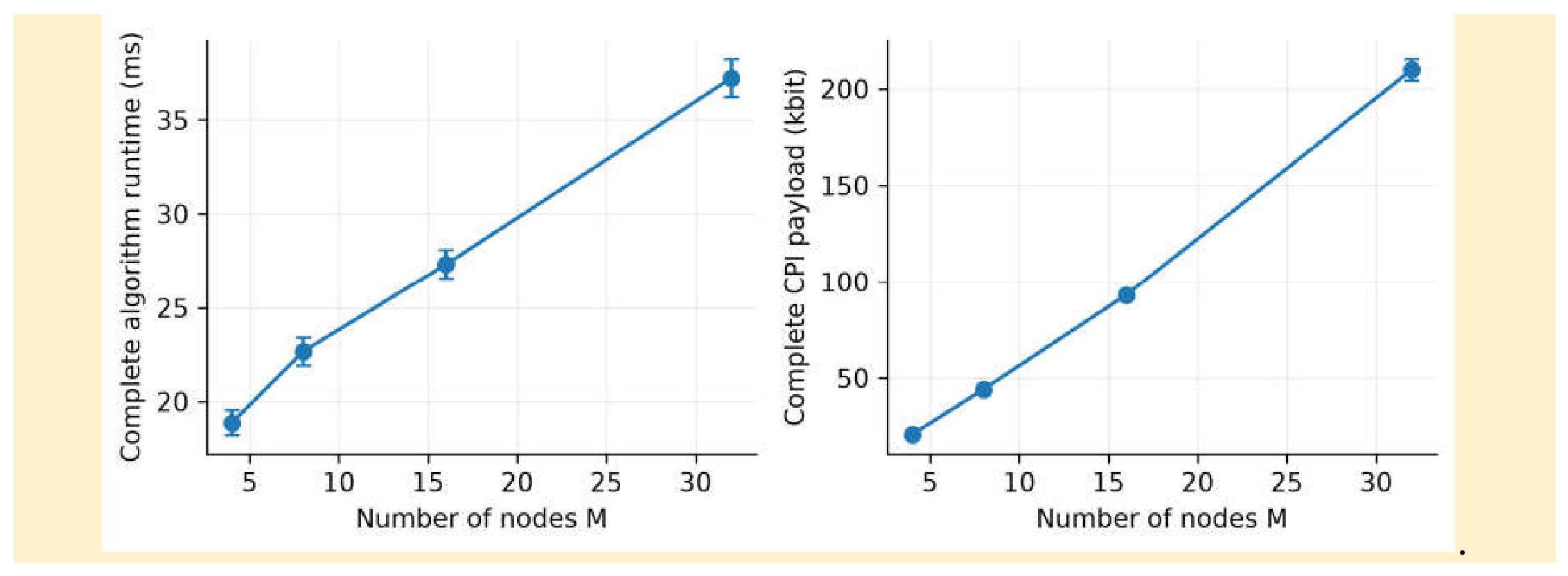
Table 12.
Matched centralized/broadcast comparisons on the same 200 core scenes. Both use one covariance refresh and three receive/power redesign rounds. All intervals are scene-wise 95% confidence intervals; central traffic is deterministic.
Table 12.
Matched centralized/broadcast comparisons on the same 200 core scenes. Both use one covariance refresh and three receive/power redesign rounds. All intervals are scene-wise 95% confidence intervals; central traffic is deterministic.
| Variant | Uploads / redesigns | Robust SINR dB and 95% CI | bit/CPI and 95% CI | Max bit/round |
|---|---|---|---|---|
| Loaded broadcast | 1 / 3 | 1.927854 [1.917683, 1.938025] | 20798.6 [20559.1, 21038.1] | 169 |
| Loaded central | 1 / 3 | 1.928028 [1.917858, 1.938198] | 20802.0 [20802.0, 20802.0] | 256 |
| SOCP broadcast | 1 / 3 | 1.974759 [1.964642, 1.984875] | 21003.9 [20774.6, 21233.2] | 169 |
| SOCP central | 1 / 3 | 1.974940 [1.964825, 1.985056] | 20802.0 [20802.0, 20802.0] | 256 |
The loaded broadcast mean is 20798.6 bit/CPI, with 95% CI [20559.1,21038.1], versus 20802 bit for the implemented compressed centralized baseline. This does not establish a meaningful traffic saving. SOCP broadcast averages 21003.9 bit/CPI. Paired robust-SINR differences favor the loaded and SOCP centralized implementations by 0.000174 dB and 0.000182 dB respectively (Table 7); these are finite implementation differences, not joint optimality gaps. Different transport precisions are explicit: q=16 scalar messages versus lossless binary64 covariance/solution transport. The former refresh-count comparison did not match redesign freshness and has been removed. The earlier 98.4% per-round and 68% complete-procedure savings are withdrawn. Payload totals exclude framing, retries, navigation updates and measured radio latency.
7.7. Phase and Geometry Sensitivity
Figure 10 evaluates three phase-error models against the stated 3 dB loss criterion. Figure 11 separately compares stale and refreshed geometry between CPIs.
Neither the common-phase model nor the phase-ramp model exceeds the mean 3 dB loss criterion at any tested angle up to 60°. For Gaussian element jitter, the first tested angle at which the mean loss exceeds this criterion is 50°. This grid does not locate an exact critical angle. Common phase does not change quadratic SINR. Changes to target amplitude, covariance, or texture can shift the practical detection boundary; no universal safe phase range is claimed. At 50°, Gaussian jitter has mean true-SINR change −3.781 dB with 95% scene-wise confidence interval [−4.365,−3.197] dB.
Geometry is held fixed within a CPI, while the drift sweep perturbs positions between CPIs. The refreshed design uses the new navigation geometry, not evaluation interference covariance. Refresh improves some cases but need not dominate in every held-out SINR realization because design optimizes a robust criterion. Large untracked within-CPI changes and packet loss remain outside the validated protocol.
7.8. Constant-Modulus Surrogate and Numerical Checks
Table 13 summarizes the numerical reference gaps at the default randomization count. Figure 12 shows their sensitivity to the number of nested candidates.
The default of 1000 candidates is an empirical computational setting, checked with nested sets of 200, 500, 1000, 2000 and 4000 draws. All 160 SDP problems and 800 recovery records are retained. The maximum primal residual is 1.68e-06; the minimum signed numerical reference gap is -7.50e-05 dB. Small negative numerical gaps are retained. Proposition 3 bounds only the fixed-Young-parameter conservative surrogate. This local fixed-power study does not establish a joint-network constant-modulus optimum or a universal randomization count.
The independent validation reconstructs all 1800 saved core W,p outputs, complete denominators, held-out SINRs, hard budgets, actual fixed-W objective gaps and applicable Equation (36) bounds. It reconciles phase and CPI traffic, checks binary32 threshold use and retained-round selection, and deliberately attempts communication-cap violations to verify rejection before send. It also recomputes paired/binomial intervals, checks solver residuals and confirms that changing held-out covariance leaves design unchanged. These tests do not prove ambiguity-set coverage or global stationarity.
8. Limitations and Applicability
The certificate is exact for the selected Wasserstein ball and stated known clutter/noise model; it does not establish that the true distribution lies in that ball. The loading approximation has no joint stationary-point or distribution-independent performance guarantee. Known clutter covariance, target gain, and calibrated geometry reduce the information burden relative to a deployment with uncertain calibration. The shared broadcast architecture avoids multihop routing and makes the tracker redundant for exact sum-budget checks. Consequently, the observed payload is not evidence of savings on sparse networks or under packet loss. Related asynchronous and federated methods [48,49,50,51] solve different coordination problems and cannot be ranked by the present counts.
The feasibility and tracking statements require F and the noise/interference offset to remain fixed during each power trial. Untracked relative motion changes coupling directions and hence F; it can alter the feasible-threshold interval and the margins in γρ(F)<1 and r=γ‖F‖∞<1. The direction of that change is geometry-dependent, and a certificate computed for the old geometry need not hold for the changed coupling. Figure 11 studies between-CPI refresh only. Within-CPI motion requires a time-varying or explicitly uncertain-coupling model, a navigation refresh schedule, and its communication and processing cost. Increasing the present external-interference Wasserstein radius alone does not certify uncertainty in the separate calibrated coupling matrices.
The detector uses 32 homogeneous reference cells and six pulses sharing a texture realization, with four guard cells excluded from estimation. Guard-cell returns do not enter the statistic and are not generated. Its threshold is calibrated on independent H0 frames and then held fixed. Texture transitions between the CUT and reference window, target-contaminated reference windows, unknown clutter covariance, and temporal correlation beyond the shared texture can invalidate this calibration. The Gaussian-energy model and CFAR covariance-estimation literature [40,52] motivate the construction but do not remove these limitations.
The constant-modulus SDP bounds a Young-inequality surrogate, not the exact robust objective. Its solver and recovery residuals must be checked; a finite randomization study does not establish a universal draw count or rank-one theorem. Phase/drift sweeps describe only their tested grid and configuration. Finally, this is a simulation study without field measurements or hardware-in-the-loop validation; platform latency, synchronization errors, navigation refresh overhead, and radio framing costs require measurement before deployment.
9. Conclusions
The complete Wasserstein worst-case quadratic form yields a valid fixed-threshold receive SOCP when normalization is handled consistently. A loaded receive update can be combined with exact-denominator power certification, but it remains an approximation to the receive block. In the stated 200-scene study, its mean true worst-node SINR is 2.663 dB and its mean robust certificate is 1.928 dB; the exact-receive branch has a 0.0469 dB higher mean certificate. Both show zero observed robust violations under the chosen ambiguity set and hard budgets. These findings do not establish distributional coverage or joint stationarity.
Quantized powers and tracker errors are coupled and have finite-resolution floors. The implemented cap is enforced before every send, and threshold flags, decisions and retained-round selection are explicitly ordered. Under the matched sample and three-redesign schedule, scalar exchange provides no demonstrated complete-CPI traffic advantage over the compressed centralized baseline. Equation (36) is checked at returned powers against a same-W continuous reference and remains conditional. Physical radio overhead, uncertain calibration, within-CPI motion and field validation remain outside the simulations.
Supplementary Materials
The following supporting information can be downloaded at the website of this paper posted on Preprints.org.
Author Contributions
Conceptualization, K.L.; Methodology, K.L.; Software, K.L., Z.D., H.W., Y.L.; Validation, Z.D., H.W., Y.W., Y.L.; Formal analysis, K.L., L.C.; Investigation, Z.D., H.W., W.L., Y.W., Yila Ma, X.L., Zihao Wang, D.L.; Writing—original draft, K.L.; Writing—review & editing, L.C.; Visualization, H.W.; Supervision, K.L., Zhilu Wu. All authors have read and agreed to the published version of the manuscript.
Funding
The authors received no specific funding for this work.
Data Availability Statement
The supplied simulation code, fixed configurations, seeds, per-trial outputs, solver, message, retained-round and power-trial ledgers, validation report, and figure-generation scripts are supplied in the accompanying Supplementary Materials package. The experiments use synthetic data; no sea-trial measurements are reported.
Acknowledgments
Doubao (ByteDance) assisted earlier code drafting and English editing. ChatGPT accessed through Codex (OpenAI; November 2026) assisted this revision with review, mathematical exposition, code revision, simulation execution, statistical analysis, and figures. The authors are responsible for verifying the final scientific content and declaring this use in the submission system. The authors acknowledge discussions with colleagues at Harbin University and Harbin Institute of Technology.
Conflicts of Interest
The authors declare no conflicts of interest.
Abbreviations
ADMM, alternating direction method of multipliers; BCD, block coordinate descent; CFAR, constant false alarm rate; CM, constant modulus; CNR, clutter-to-noise ratio; CPI, coherent processing interval; CUT, cell under test; DRFM, digital radio frequency memory; DRO, distributionally robust optimization; JNR, jamming-to-noise ratio; JSR, jammer-to-signal ratio (legacy label only; the implementation uses an interference-to-noise scale, as specified in Section 7.1); KKT, Karush–Kuhn–Tucker; LMI, linear matrix inequality; MPDR, minimum power distortionless response; MVDR, minimum variance distortionless response; RCS, radar cross section; SDP, semidefinite programming; SDR, semidefinite relaxation; SINR, signal-to-interference-plus-noise ratio; SOCP, second-order cone programming; ULA, uniform linear array.
Appendix A. Worst-Case Form and SOCP Equivalence
Write a = ‖w‖² and c = E|wᴴj|². For any coupling (j,z) of the empirical measure and a candidate distribution with E‖z−j‖² ≤ ε, the L² triangle inequality and Cauchy–Schwarz give the upper bound below.
For a,c,ε > 0, choose the deterministic transport below. Its expected squared displacement is ε, and its projection onto w has a common positive multiplicative factor, attaining the upper bound. If c = 0 and a > 0, a displacement of length √ε parallel to w attains aε. If a = 0 or ε = 0, the result is immediate.
This proves Lemma 2 without a covariance-coverage assumption. For Proposition 2, divide a weight with a nonzero target response by a(0)ᴴw; the SINR is unchanged. Applying (15), the inequality Γ ≥ γ becomes φε(w)+wᴴQw ≤ |α|²pG/γ. Introducing t at least the sum of the two norms gives exactly (18). Conversely, any point satisfying (18) satisfies the original inequality because t is nonnegative and bounds that sum. Positive thermal noise excludes unbounded beneficial scaling. Returning w/‖w‖ changes neither the ratio nor its certificate. No matrix containing λw or γp is described as a jointly affine LMI.
Appendix B. Scope of the Constant-Modulus SDP
Young’s inequality 2xy ≤ ηYx² + y²/ηY applied to x = √(wᴴR̂w), y = √ε‖w‖ gives the conservative denominator AηY. A constant-modulus weight yields X ≽ 0, diag X = 1/na, and rank X = 1. Dropping the rank-one constraint enlarges the conservative feasible set. Since AηY is positive definite, tr(AηYX) > 0, and the Charnes–Cooper substitution is reversible with z > 0. In (21), z = 0 would force a positive-semidefinite Y with zero diagonal to vanish, contradicting tr(AηYY) = 1. Thus (21) is a valid convex SDP. Its upper-bound statement is limited to the conservative surrogate. Recovered phase-only vectors satisfy the original constant-modulus equality, but no approximation ratio for the exact robust objective follows.
Appendix C. Coupled Recursion and Gap Proof
Subtract p* = γ(Fp*+v) from the quantized update to obtain (28). Iteration and the induced infinity norm yield the geometric series in (29). Premultiplying the tracker recursion by 1ᵀ removes (Wc−I)Qh(h), proving mean preservation from h0 = p0. Applying I−J then yields (30). Symmetry and double stochasticity imply the operator norm bound λ on the disagreement subspace. Iterating the driven recursion gives (31); using pnew−p = (γF−I)e + ηp gives (32), and taking limits yields (33). These inequalities are conditional on the stated norm contraction and absence of saturation; timeout and saturation are implementation statuses, not silently discarded events.
For fm(p) = pm/((Fp)m+vm), subtracting two fractions and using the lower bound vmin on their denominators and the upper bound Pmax on their numerators gives |fm(p)−fm(p′)| ≤ LW‖p−p′‖∞. Taking a minimum preserves this Lipschitz bound. At the positive fixed point for γ, each fm equals γ. Therefore |gW(pT)−γ| ≤ LW ET. Combining this with the definition of γW* and physical feasibility of pT proves (36). The term γW*−γ explicitly retains threshold backoff; it includes no claim about optimal receive weights or true-covariance design.
Appendix D. Objective Values and Reproducibility Checks
With ideal exact blocks, the previous feasible pair W,p can be retained when a block is updated. The objective cannot decrease, and the noise-only bound from Section 5.1 bounds it above. Hence the sequence of objective values converges. This proof supplies no joint stationarity result. For the finite implemented schedule, retaining the iterate with the highest accepted threshold proves only that the selected output is no worse under its accepted-threshold metric than the other saved iterates. Independent residual evaluation is still required. The released validation script checks raw residuals, hard budgets, the tracker mean invariant, paired-interval recomputation, binomial counts, and common Table 11 provenance. It also verifies that the design API does not accept evaluation covariance.
References
- Hu, J.; Ding, J.; Zhou, F.; Zhang, Y.; Zhou, C.; Qu, C. A survey on autonomous coordination technology for radar networks. J. Radars 2026, 15, 1059–1090. (in Chinese). [Google Scholar]
- Ding, H.; Dong, Y.; Liu, N.; Wang, G.; Guan, J. Overview and prospects of research on sea clutter property cognition. J. Radars (in Chinese). 2016, 5, 499–516. [Google Scholar] [CrossRef]
- He, B.; Su, H. A review of game theory analysis in cognitive radar anti-jamming. J. Electron. Inf. Technol. (in Chinese). 2021, 43, 1199–1211. [Google Scholar] [CrossRef]
- Liu, L.; Liang, X.; Li, Y.; Zeng, Z.; Tang, H. A novel joint radar-communication waveform design method based on distributed aperture. J. Radars (in Chinese). 2023, 12, 297–311. [Google Scholar] [CrossRef]
- Yuan, Y.; Liu, X.; Li, W.; Yi, W.; Choi, W. Decentralized resource allocation for multi-radar systems based on quality of service framework. IEEE Trans. Signal Process. 2024, 72, 1189–1204. [Google Scholar] [CrossRef]
- Ma, Y.; Chen, S.; Xing, C.; Bu, X.; Hanzo, L. Decomposition optimization algorithms for distributed radar systems. IEEE Trans. Signal Process. 2016, 64, 6443–6458. [Google Scholar] [CrossRef]
- Han, K.; Meng, K.; Wang, X.-Y.; Masouros, C. Network-level ISAC design: State-of-the-art, challenges, and opportunities. IEEE J. Sel. Top. Electromagn. Antennas Propag. 2025, 1, 65–83. [Google Scholar] [CrossRef]
- Liu, Z.; Liu, X.; Liu, Y.; Leung, V.C.M.; Durrani, T.S. UAV assisted integrated sensing and communications for Internet of Things: 3D trajectory optimization and resource allocation. IEEE Trans. Wirel. Commun. 2024, 23, 8654–8667. [Google Scholar] [CrossRef]
- Yu, X.; Alhujaili, K.; Cui, G.; Monga, V. MIMO radar waveform design in the presence of multiple targets and practical constraints. IEEE Trans. Signal Process. 2020, 68, 1974–1989. [Google Scholar] [CrossRef]
- Wu, L.; Babu, P.; Palomar, D.P. Transmit waveform/receive filter design for MIMO radar with multiple waveform constraints. IEEE Trans. Signal Process. 2018, 66, 1526–1540. [Google Scholar] [CrossRef]
- Hua, H.; Xu, J.; Han, T.X. Optimal transmit beamforming for integrated sensing and communication. IEEE Trans. Veh. Technol. 2023, 72, 10588–10603. [Google Scholar] [CrossRef]
- Zou, J.; Sun, S.; Masouros, C.; Cui, Y.; Liu, Y.-F.; Ng, D.W.K. Energy-efficient beamforming design for integrated sensing and communications systems. IEEE Trans. Commun. 2024, 72, 3766–3782. [Google Scholar] [CrossRef]
- Delage, E.; Ye, Y. Distributionally robust optimization under moment uncertainty with application to data-driven problems. Oper. Res. 2010, 58, 595–612. [Google Scholar] [CrossRef]
- Mohajerin Esfahani, P.; Kuhn, D. Data-driven distributionally robust optimization using the Wasserstein metric: Performance guarantees and tractable reformulations. Math. Program. 2018, 171, 115–166. [Google Scholar] [CrossRef]
- Irani, K.H.; Huang, Y.; Vorobyov, S.A. SINR maximizing distributionally robust adaptive beamforming. IEEE Trans. Signal Process. 2025, 73, 2542–2557. [Google Scholar] [CrossRef]
- Wang, S.; Dai, W.; Li, G.Y. Distributionally robust adaptive beamforming. IEEE Trans. Signal Process. 2025, 73, 2981–2997. [Google Scholar] [CrossRef]
- Deng, W.; Yin, W. On the global and linear convergence of the generalized alternating direction method of multipliers. J. Sci. Comput. 2016, 66, 889–916. [Google Scholar] [CrossRef]
- Boyd, S.; Parikh, N.; Chu, E.; Peleato, B.; Eckstein, J. Distributed optimization and statistical learning via the alternating direction method of multipliers. Found. Trends Mach. Learn. 2011, 3, 1–122. [Google Scholar] [CrossRef]
- He, M.; Jia, Y.; Greco, M.S.; Gini, F.; Wang, W.-Q. Transmit waveform design based on ambiguity function shaping for distributed coherent aperture radar in MIMO mode. IEEE Geosci. Remote Sens. Lett. 2024, 21, 1–5. [Google Scholar] [CrossRef]
- Cheng, X.; Li, M.; Ciuonzo, D.; Wang, F.; Gong, P.; Wu, Y. Suppressing interrupted sampling repeater jamming by transceiver design of fully-polarimetric wideband radars. IEEE Sens. J. 2024, 24, 41572–41584. [Google Scholar] [CrossRef]
- Li, Z.; Hu, F.; Li, Q.; Ling, Z.; Chang, Z.; Hämäläinen, T. AoI-aware waveform design for cooperative joint radar-communications systems with online prediction of radar target property. IEEE Trans. Commun. 2024, 72, 6029–6043. [Google Scholar] [CrossRef]
- Vorobyov, S.A.; Gershman, A.B.; Luo, Z.-Q. Robust adaptive beamforming using worst-case performance optimization: A solution to the signal mismatch problem. IEEE Trans. Signal Process. 2003, 51, 313–324. [Google Scholar] [CrossRef]
- Li, J.; Stoica, P.; Wang, Z. On robust Capon beamforming and diagonal loading. IEEE Trans. Signal Process. 2003, 51, 1702–1715. [Google Scholar] [CrossRef]
- Yates, R.D. A framework for uplink power control in cellular radio systems. IEEE J. Sel. Areas Commun. 1995, 13, 1341–1347. [Google Scholar] [CrossRef]
- Schubert, M.; Boche, H. Solution of the multiuser downlink beamforming problem with individual SINR constraints. IEEE Trans. Veh. Technol. 2004, 53, 18–28. [Google Scholar] [CrossRef]
- Qi, C.; Xie, J.; Zhang, H. Joint antenna placement and power allocation for target detection in a distributed MIMO radar network. Remote Sens. 2022, 14, 2650. [Google Scholar] [CrossRef]
- Bounaceur, H.; Khenchaf, A.; Le Caillec, J.-M. Analysis of small sea-surface targets detection performance according to airborne radar parameters in abnormal weather environments. Sensors 2022, 22, 3263. [Google Scholar] [CrossRef]
- Rahman, S.; Vattulainen, A.B.; Robertson, D.A. Doppler characteristics of sea clutter at K-band and W-band: Results from the St Andrews and Coniston Water trials. In Proceedings of the 2023 IEEE International Radar Conference (RADAR), Sydney, Australia, 6–10 November 2023; pp. 1–6. [Google Scholar] [CrossRef]
- Yue, M.-C.; Rychener, Y.; Kuhn, D.; Nguyen, V.A. A geometric unification of distributionally robust covariance estimators: Shrinking the spectrum by inflating the ambiguity set. Oper. Res. 2026, 74, 1710–1728. [Google Scholar]
- Wang, Z.; Glynn, P.W.; Ye, Y. Likelihood robust optimization for data-driven problems. Comput. Manag. Sci. 2016, 13, 241–261. [Google Scholar] [CrossRef]
- He, S.; Zheng, J.; Feng, M.; Chen, Y. Communication-efficient federated learning with adaptive consensus ADMM. Appl. Sci. 2023, 13, 5270. [Google Scholar] [CrossRef]
- Ben Issaid, C.; Elgabli, A.; Park, J.; Bennis, M.; Debbah, M. Communication-efficient decentralized learning over bipartite graphs. IEEE Trans. Wirel. Commun. 2022, 21, 4150–4167. [Google Scholar] [CrossRef]
- Yi, X.; Zhang, S.; Yang, T.; Chai, T.; Johansson, K.H. Sublinear and linear convergence of modified ADMM for distributed nonconvex optimization. IEEE Trans. Control Netw. Syst. 2023, 10, 75–86. [Google Scholar] [CrossRef]
- Di Lorenzo, P.; Scutari, G. NEXT: In-network nonconvex optimization. IEEE Trans. Signal Inf. Process. Netw. 2016, 2, 120–136. [Google Scholar] [CrossRef]
- Sayed, A.H. Adaptation, learning, and optimization over networks. Found. Trends Mach. Learn. 2014, 7, 311–801. [Google Scholar] [CrossRef]
- Huang, Y. Challenges and opportunities of sub-6 GHz integrated sensing and communications for 5G-advanced and beyond. Chin. J. Electron. 2024, 33, 323–325. [Google Scholar] [CrossRef]
- Liu, A.; Huang, Z.; Li, M.; Wan, Y.; Li, W.; Han, T.X.; Liu, C.; Du, R.; Tan, D.K.P.; Lu, J.; Shen, Y.; Colone, F.; Chetty, K. A survey on fundamental limits of integrated sensing and communication. IEEE Commun. Surv. Tutor. 2022, 24, 994–1034. [Google Scholar] [CrossRef]
- Liu, F.; Cui, Y.; Masouros, C.; Xu, J.; Han, T.X.; Eldar, Y.C.; Buzzi, S. Integrated sensing and communications: Toward dual-functional wireless networks for 6G and beyond. IEEE J. Sel. Areas Commun. 2022, 40, 1728–1767. [Google Scholar] [CrossRef]
- Liyanaarachchi, S.D.; Riihonen, T.; Baquero Barneto, C.; Valkama, M. Joint MIMO communications and sensing with hybrid beamforming architecture and OFDM waveform optimization. IEEE Trans. Wirel. Commun. 2024, 23, 1565–1580. [Google Scholar] [CrossRef]
- Ward, K.D.; Watts, S. Use of sea clutter models in radar design and development. IET Radar Sonar Navig. 2010, 4, 146–157. [Google Scholar] [CrossRef]
- Ledoit, O.; Wolf, M. Honey, I shrunk the sample covariance matrix. J. Portf. Manag. 2004, 30, 110–119. [Google Scholar] [CrossRef]
- Soltanalian, M.; Stoica, P. Designing unimodular codes via quadratic optimization. IEEE Trans. Signal Process. 2014, 62, 1221–1234. [Google Scholar] [CrossRef]
- Aubry, A.; De Maio, A.; Piezzo, M.; Farina, A. Radar waveform design in a spectrally crowded environment via nonconvex quadratic optimization. IEEE Trans. Aerosp. Electron. Syst. 2014, 50, 1138–1152. [Google Scholar] [CrossRef]
- Shi, W.; Ling, Q.; Wu, G.; Yin, W. A proximal gradient algorithm for decentralized composite optimization. IEEE Trans. Signal Process. 2015, 63, 6013–6023. [Google Scholar] [CrossRef]
- Nedić, A.; Olshevsky, A.; Rabbat, M.G. Network topology and communication-computation tradeoffs in decentralized optimization. Proc. IEEE 2018, 106, 953–976. [Google Scholar] [CrossRef]
- Boyd, S.; Ghosh, A.; Prabhakar, B.; Shah, D. Randomized gossip algorithms. IEEE Trans. Inf. Theory 2006, 52, 2508–2530. [Google Scholar] [CrossRef]
- Kempe, D.; Dobra, A.; Gehrke, J. Gossip-based computation of aggregate information. In Proceedings of the 44th Annual IEEE Symposium on Foundations of Computer Science (FOCS), Cambridge, MA, USA, 11–14 October 2003; pp. 482–491. [Google Scholar] [CrossRef]
- Chang, T.-H.; Hong, M.; Liao, W.-C.; Wang, X. Asynchronous distributed ADMM for large-scale optimization—Part I: Algorithm and convergence analysis. IEEE Trans. Signal Process. 2016, 64, 3118–3130. [Google Scholar] [CrossRef]
- Wei, E.; Ozdaglar, A. On the O(1/k) convergence of asynchronous distributed alternating direction method of multipliers. In Proceedings of the IEEE Global Conference on Signal and Information Processing (GlobalSIP), 2013; pp. 551–554. [Google Scholar] [CrossRef]
- McMahan, H.B.; Moore, E.; Ramage, D.; Hampson, S.; Agüera y Arcas, B. Communication-efficient learning of deep networks from decentralized data. In Proceedings of the 20th International Conference on Artificial Intelligence and Statistics (AISTATS), Fort Lauderdale, FL, USA, 20–22 April 2017; PMLR 54, pp. 1273–1282. Available online: https://proceedings.mlr.press/v54/mcmahan17a.html.
- Li, T.; Sahu, A.K.; Zaheer, M.; Sanjabi, M.; Talwalkar, A.; Smith, V. Federated optimization in heterogeneous networks. In Proceedings of the 3rd Annual Conference on Machine Learning and Systems (MLSys), Austin, TX, USA, 2020; pp. 429–450. Available online: https://proceedings.mlsys.org/paper_files/paper/2020/hash/1f5fe83998a09396ebe6477d9475ba0c-Abstract.html.
- Gini, F.; Greco, M. Covariance matrix estimation for CFAR detection in correlated heavy-tailed clutter. Signal Process. 2002, 82, 1847–1859. [Google Scholar] [CrossRef]
Figure 1.
Reliable broadcast implementation with three fixed outer rounds. Design uses local training and calibrated geometry; held-out covariance is accessed only after design. All threshold trials contribute to the communication ledger.
Figure 1.
Reliable broadcast implementation with three fixed outer rounds. Design uses local training and calibrated geometry; held-out covariance is accessed only after design. All threshold trials contribute to the communication ledger.
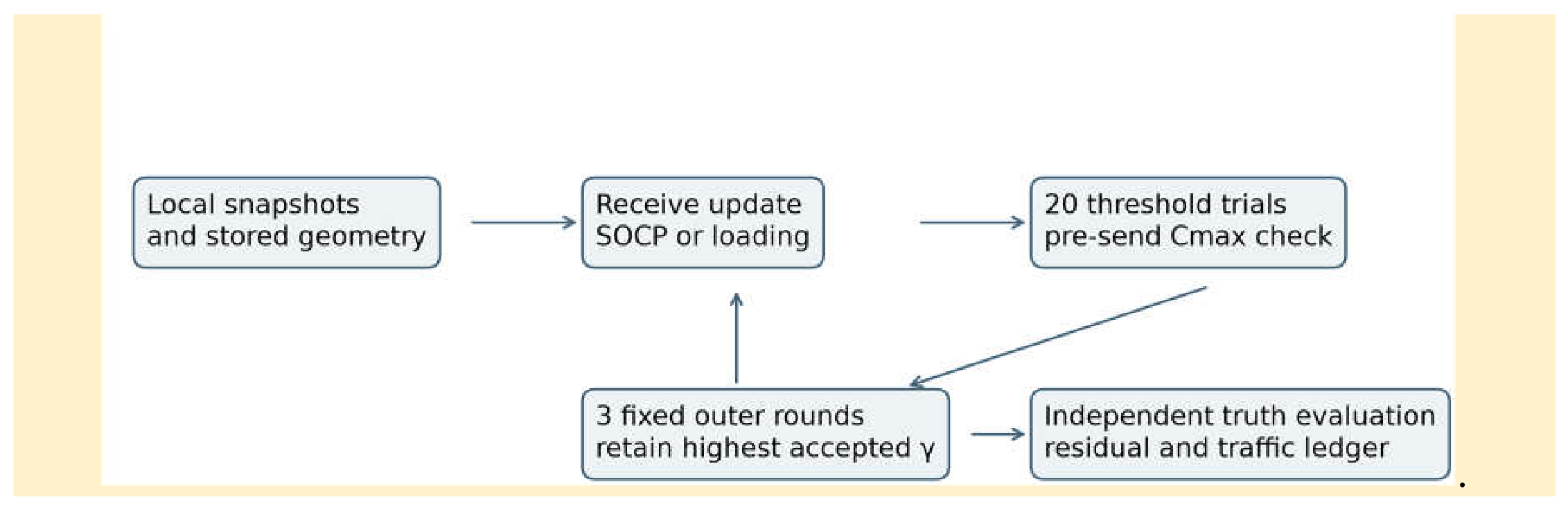
Figure 2.
True and exact worst-case SINR of final joint outputs. Error bars are 95% confidence intervals across scenes; no global-optimum interpretation is attached to the SOCP receive branch.
Figure 2.
True and exact worst-case SINR of final joint outputs. Error bars are 95% confidence intervals across scenes; no global-optimum interpretation is attached to the SOCP receive branch.
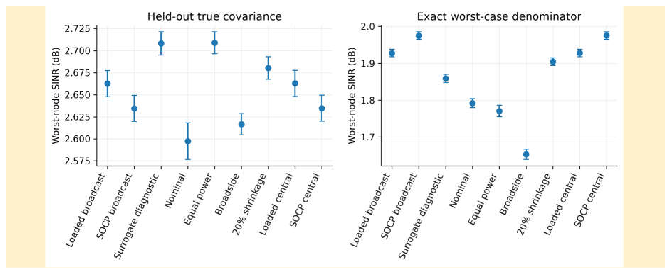
Figure 3.
Accepted threshold trial associated with the retained outer round at seed 10000. Power feasibility residual and tracker disagreement are distinct; these are not means across 200 scenes. The released outer index and accepted trial identify the plotted record.
Figure 3.
Accepted threshold trial associated with the retained outer round at seed 10000. Power feasibility residual and tracker disagreement are distinct; these are not means across 200 scenes. The released outer index and accepted trial identify the plotted record.
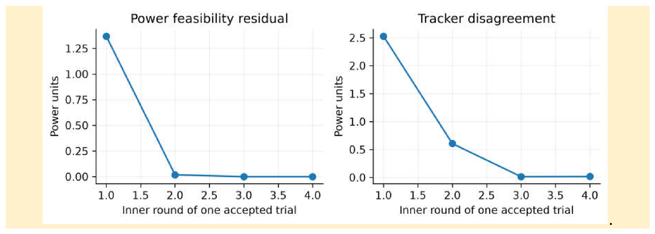
Figure 4.
Same-weight, same-sample continuous-power gap and complete CPI payload versus q (40 scenes). The gap is not a joint global-optimality gap.
Figure 4.
Same-weight, same-sample continuous-power gap and complete CPI payload versus q (40 scenes). The gap is not a joint global-optimality gap.
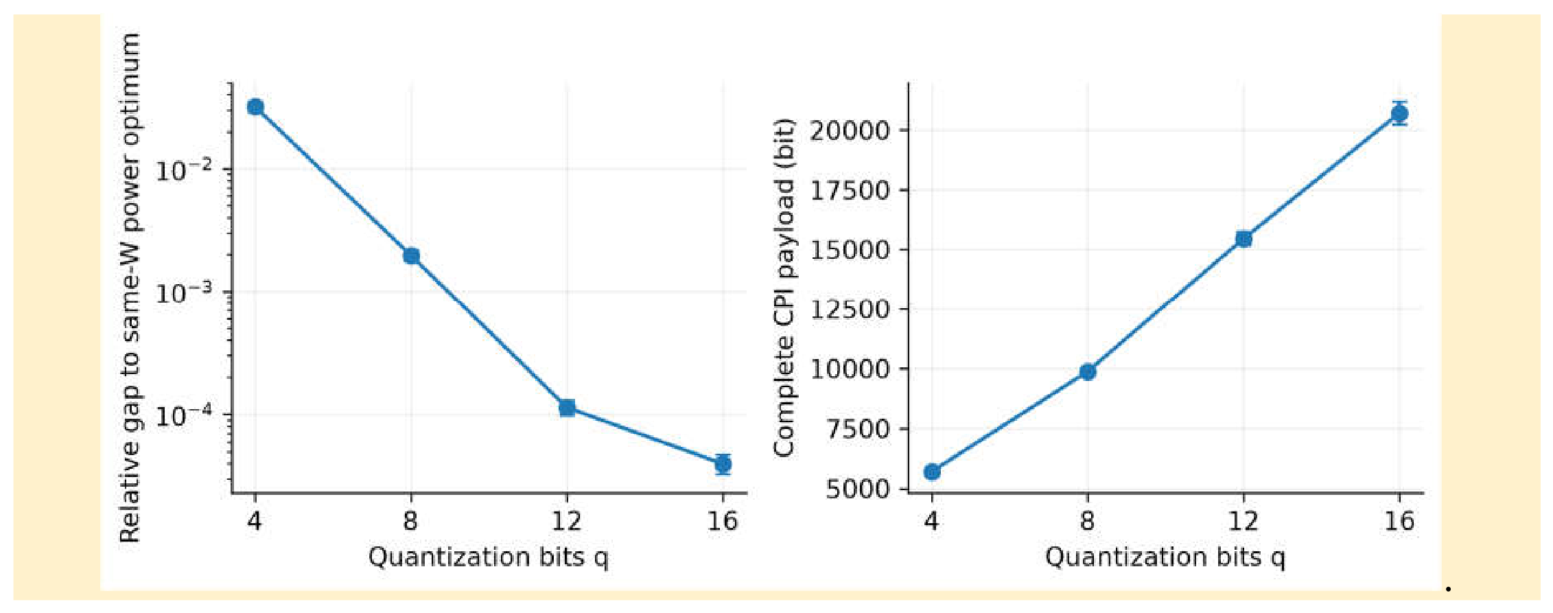
Figure 5.
Held-out true SINR versus training length, 40 seeds per setting. Error bars are 95% confidence intervals across scenes. Shrinkage uses a fixed 20% coefficient.
Figure 5.
Held-out true SINR versus training length, 40 seeds per setting. Error bars are 95% confidence intervals across scenes. Shrinkage uses a fixed 20% coefficient.
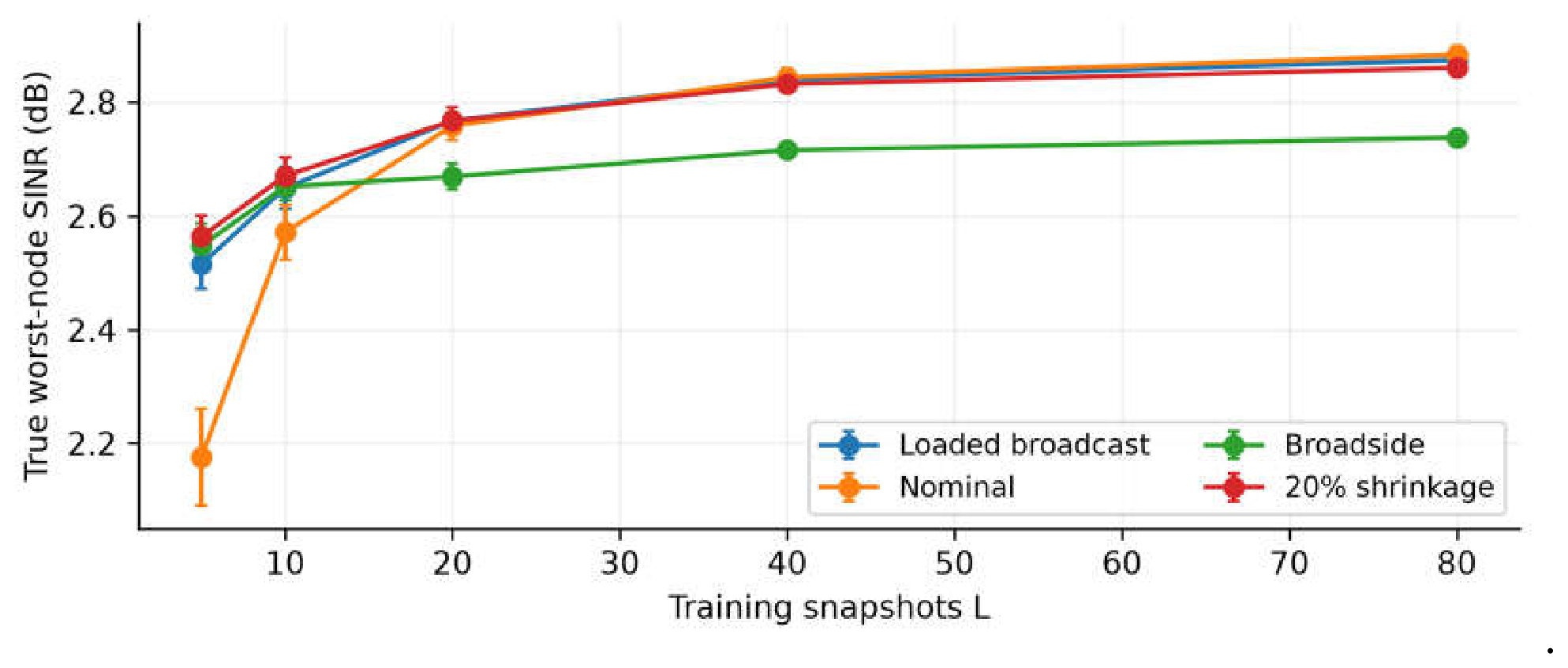
Figure 6.
True SINR and the corresponding certificate for the selected radius as the engineering radius changes. A smaller radius defines a weaker uncertainty set, so certificates across radii are not guarantees for a common ambiguity set.
Figure 6.
True SINR and the corresponding certificate for the selected radius as the engineering radius changes. A smaller radius defines a weaker uncertainty set, so certificates across radii are not guarantees for a common ambiguity set.
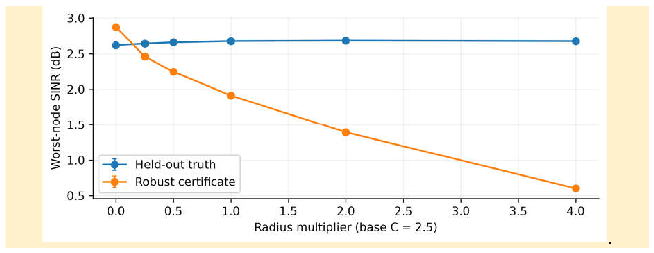
Figure 7.
Independent H0/H1 counts after one independent threshold calibration. Intervals are conditional on that fixed threshold. The design scene is seed 10000; these are not averages over 200 scene designs.
Figure 7.
Independent H0/H1 counts after one independent threshold calibration. Intervals are conditional on that fixed threshold. The design scene is seed 10000; these are not averages over 200 scene designs.
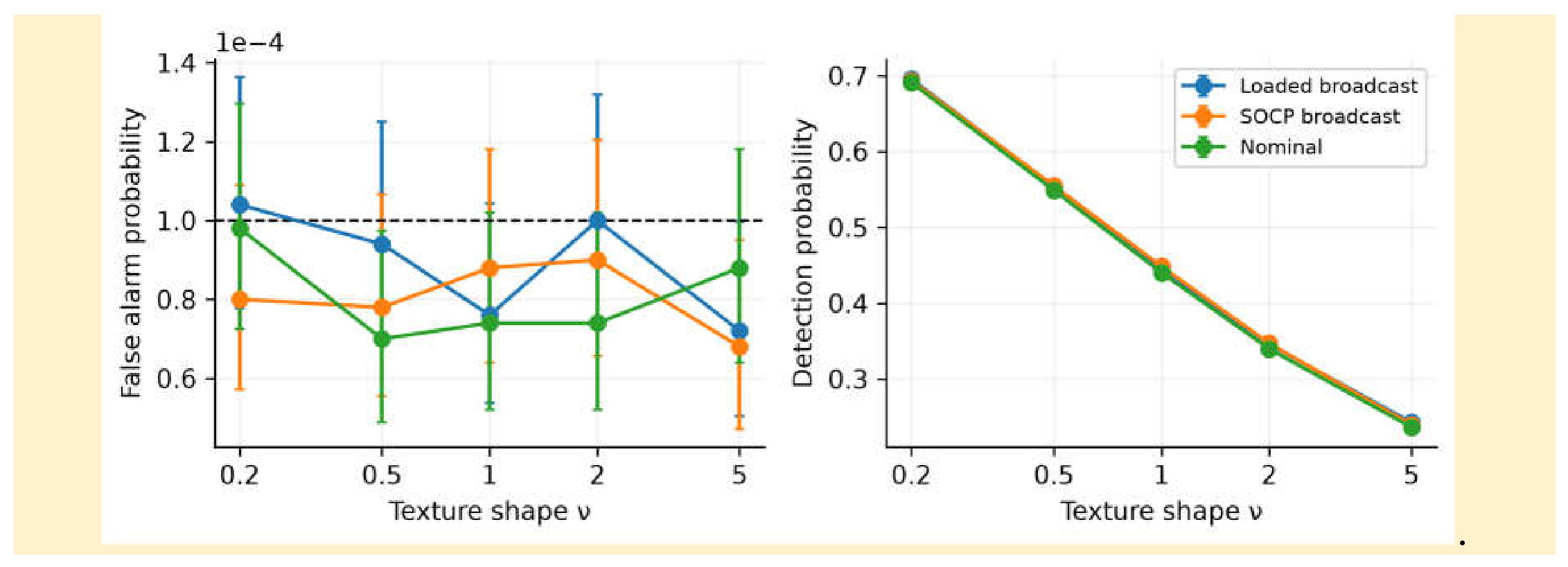
Figure 9.
Complete-CPI payload of matched alternating designs: the same training covariance, one refresh, and three receive/power redesign rounds. Broadcast powers/trackers use q=16; central covariance and final weights/powers use binary64 transport. Error bars are scene-wise 95% confidence intervals.
Figure 9.
Complete-CPI payload of matched alternating designs: the same training covariance, one refresh, and three receive/power redesign rounds. Broadcast powers/trackers use q=16; central covariance and final weights/powers use binary64 transport. Error bars are scene-wise 95% confidence intervals.
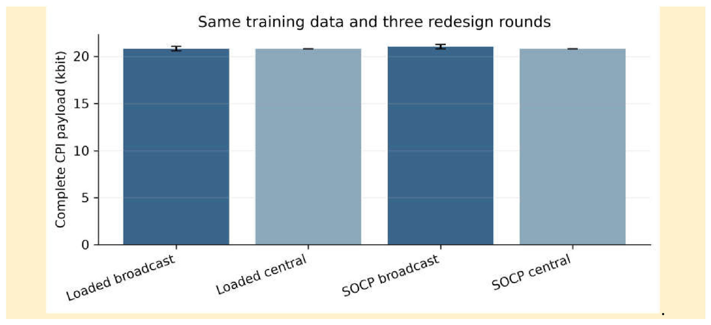
Figure 10.
Phase scan through 60°: common phase; a deterministic ramp from −θ to +θ across elements; independent Gaussian element jitter with standard deviation θ. Breakdown is a mean true-SINR loss greater than 3 dB relative to the zero-error design.
Figure 10.
Phase scan through 60°: common phase; a deterministic ramp from −θ to +θ across elements; independent Gaussian element jitter with standard deviation θ. Breakdown is a mean true-SINR loss greater than 3 dB relative to the zero-error design.
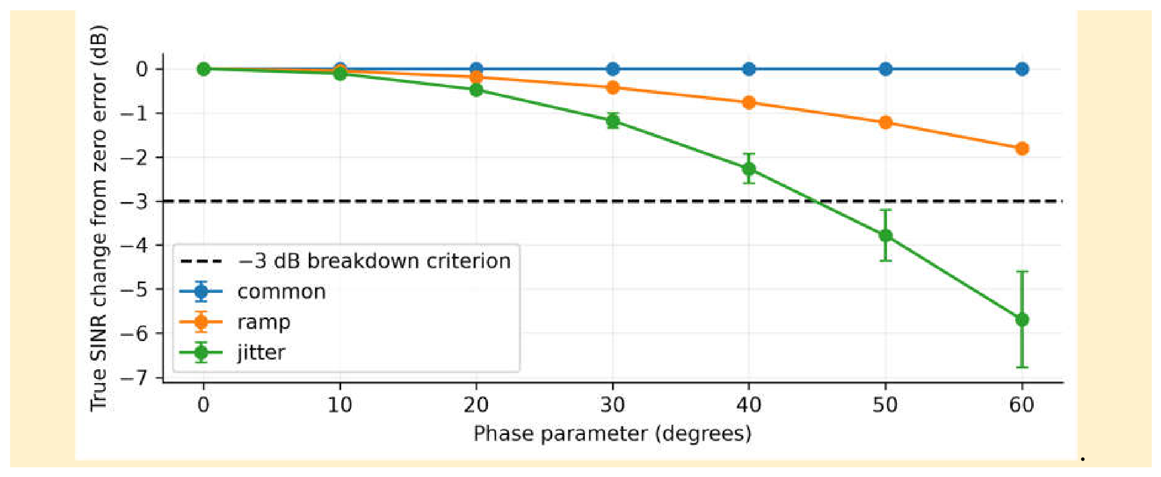
Figure 11.
Stale geometry versus redesign with refreshed coupling directions, 40 paired scenes at each drift. Training and evaluation interference covariances otherwise remain unchanged. Positions use normalized deployment units.
Figure 11.
Stale geometry versus redesign with refreshed coupling directions, 40 paired scenes at each drift. Training and evaluation interference covariances otherwise remain unchanged. Positions use normalized deployment units.
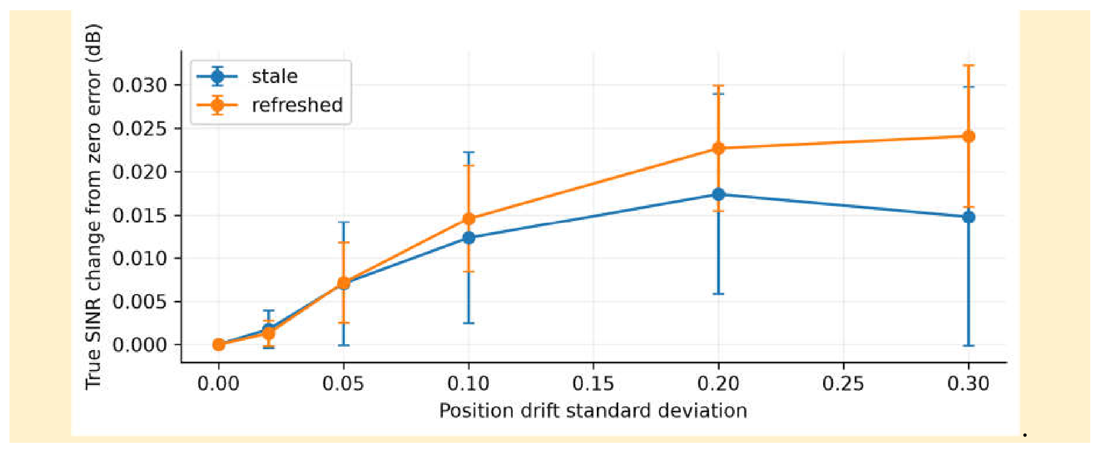
Figure 12.
Nested Gaussian randomization for the fixed-Young-parameter conservative surrogate. SCS objectives are numerical reference values; no certified dual upper bound is claimed for finite-precision solver outputs.
Figure 12.
Nested Gaussian randomization for the fixed-Young-parameter conservative surrogate. SCS objectives are numerical reference values; no certified dual upper bound is claimed for finite-precision solver outputs.
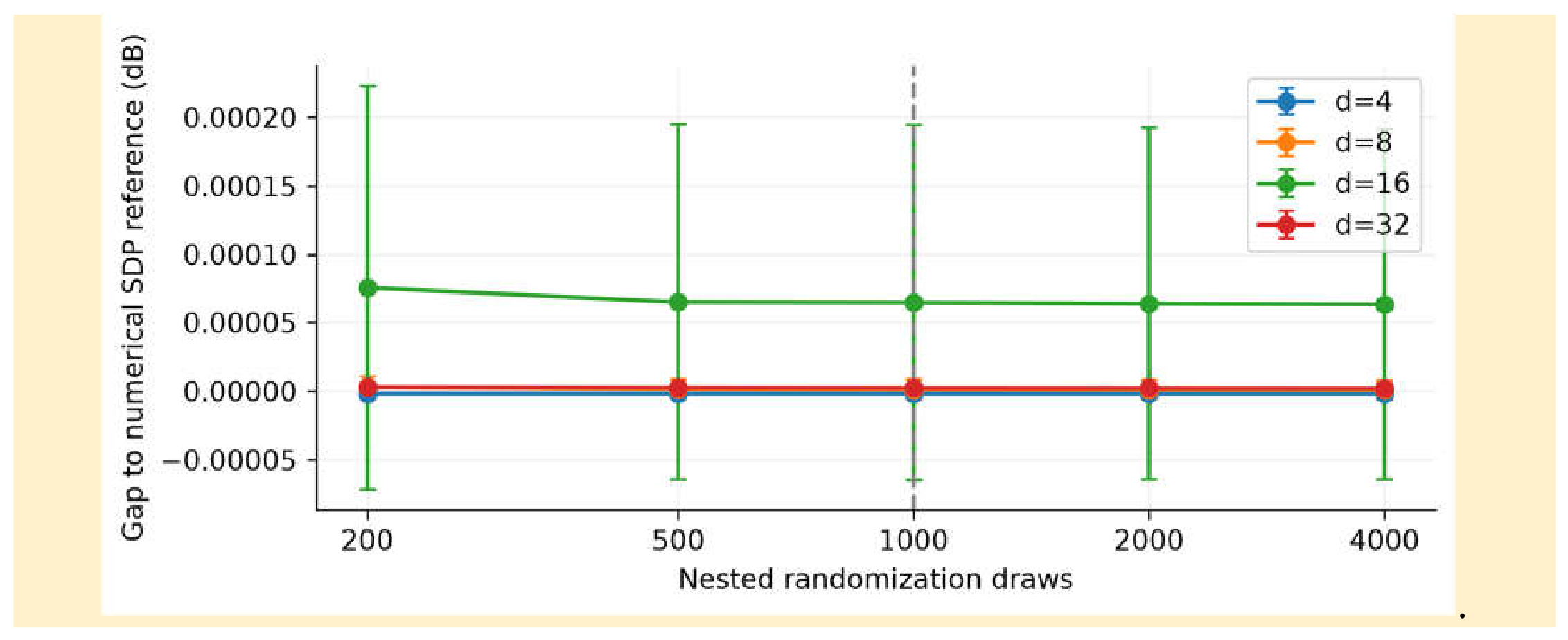
Table 1.
Comparison of this work with closely related work.
| Representative work | Uncertainty description | Architecture or scope | Communication limit | Adaptive variables | Guarantee used here |
|---|---|---|---|---|---|
| Waveform/filter design [9,10]; ISAC [11] | Application-specific; no common DRO model inferred | Central design problems | No limit inferred from these citations | Waveforms, filters, or transmit beams | No distributed claim imported |
| Resource allocation [5,6,8] | Use each paper’s stated model | Network resource allocation | Application-specific | Resources and related variables | No generic limited-sample guarantee imported |
| ADMM [17,18]; cooperative waveform [21] | Algorithm framework or separate application | Application-specific coordination | Message sizes require implementation | Primal/dual or waveform variables | Assumption-dependent convergence |
| This work | Squared W2 ball; engineering radius | Reliable shared broadcast | Cmax enforced before each send | Receive weights and powers; codes fixed | Conditional fixed-W power bound |
Table 2.
Itemized comparison with existing DRO and distributed ADMM methods.
| Method | Uncertainty model | Communication scope | Adaptive beam or code | Network power | Scope of statement |
|---|---|---|---|---|---|
| General DRO [14] | Empirical Wasserstein ball | Not a radar protocol | General decision variables | Application-dependent | Guarantees require stated assumptions |
| Irani et al. [15] | INC support/mean/similarity; steering moments | Single-beam formulation | Receive beam; uncertain steering | No network power protocol | Conic duality and LMI relaxation |
| Wang et al. [16] | Snapshot/IPN covariance; local/global DRO | Beamforming framework | Robust receive beam | No present broadcast protocol | Regularized/Bayesian relations under stated models |
| ADMM [6,17,18] | Specified by the application | Primal/dual or consensus messages | Application-dependent | Application-dependent | No universal traffic or uncertainty model |
| This work | Squared W2 ball; known calibration | Reliable broadcast; numeric cap | Receive weights; fixed codes | Coupled max–min | Exact local SOCP; conditional power gap |
Table 3.
Main notation.
| Symbol | Meaning | Symbol | Meaning |
|---|---|---|---|
| M/N | Number of nodes / transmit code length (processing gain G = N) | na | Number of antenna elements per node (beamforming dimension) |
| L | Number of effective interference snapshots | np | Number of pulses for noncoherent integration |
| wm/pm | Receive beamforming weight / transmit power of node m | W/p | Beamforming weight matrix / power vector |
| a(u) | Array steering vector in direction u = sinθ | Matched steering in the target boresight direction | |
| RJ,m (true) / RJ,m (sample) | True / sample interference covariance | Rc,m | Sea-clutter speckle covariance |
| αm | Target complex gain (including RCS and two-way attenuation) | β2 | Link isolation factor (about −20 dB) |
| Cmax/Bt | Per-round backhaul budget / actual number of bits exchanged in round t | q | Number of bits per uniformly quantized scalar |
| γ/ϵ | Auxiliary worst-node SINR variable / Wasserstein radius | λm / Wc | Quadratic-loss dual multiplier / doubly stochastic mixing matrix |
| β | Link-isolation amplitude factor in (3) (β² ≈ 0.01, about −20 dB; Section 3.2) | ζ, C | Radius tuning parameter and calibration constant in (14) (engineering calibration, not a confidence level; Proposition 1) |
| h / ηY | Local budget tracker / fixed parameter in Young’s inequality | Δu | Angular drift of the interference direction relative to the training direction |
| χmk / umk | Code cross-correlation / interference direction from node k | zc,m | K-distributed sea clutter (compound Gaussian) |
Table 4.
Implemented controlled variants. All use the same local samples and calibrated geometry.
| Variant | Receive update | Power denominator / coordination |
|---|---|---|
| Loaded broadcast | Loaded inverse | Exact / q-bit broadcast |
| SOCP broadcast | Exact local SOCP | Exact / q-bit broadcast |
| Surrogate diagnostic | Loaded inverse | Reduced / q-bit broadcast |
| Nominal | Sample inverse | Nominal / q-bit broadcast |
| Equal power | Loaded inverse | Fixed power |
| Broadside | Fixed steering | Exact / q-bit broadcast |
| 20% shrinkage | Fixed shrinkage | Exact / q-bit broadcast |
| Loaded central | Loaded inverse | Exact / continuous central |
| SOCP central | Exact local SOCP | Exact / continuous central |
Table 5.
Fixed configuration and trial units.
| Item | Setting |
|---|---|
| Network and array | M=4, d=8, N=G=64; reliable shared broadcast |
| Power and calibration | Pmax=100 W; Ptot=300 W; σn²=1; |α|=.14 |
| Isolation and clutter | β²=.01; Gβ²=.64; known CNR=10 dB; correlation length 4 |
| Training and radius | L=10; nominal interference scale 20 dB relative to noise; C=2.5; ζ=.05 |
| Iterations | 3 outer; 20 threshold trials per outer; ≤200 inner per trial |
| Quantization | q=16; power range [0,100]; tracker range [−1600,1600] |
| Trials | Core: 200 paired scenes; each parameter setting: 40 scenes |
| Constant modulus | Young parameter ηY=1; default Nrand=1000; nested 200–4000 |
| Detector | 6 pulses; 32 reference cells; 4 excluded guard cells; Pfa=10⁻⁴ |
| Communication cap | Main Cmax=256 bit/complete round; scaling Cmax=64M; pre-send enforcement |
| Central transport | One binary64 Hermitian upload; same 3 redesigns; binary64 W,p,threshold return |
| Retention | Largest accepted threshold; latest tie; final reports occur after selection |
Table 10.
Detector counts and exact 95% confidence intervals for certified loading. H1 uses 100000 trials per setting.
Table 10.
Detector counts and exact 95% confidence intervals for certified loading. H1 uses 100000 trials per setting.
| ν | H0 count / n | Pfa and interval | Pd and interval |
|---|---|---|---|
| 0.2 | 52/500000 | 0.000104 [0.000078, 0.000136] | 0.6957 [0.6928, 0.6985] |
| 0.5 | 47/500000 | 0.000094 [0.000069, 0.000125] | 0.5534 [0.5503, 0.5565] |
| 1.0 | 38/500000 | 0.000076 [0.000054, 0.000104] | 0.4447 [0.4417, 0.4478] |
| 2.0 | 50/500000 | 0.000100 [0.000074, 0.000132] | 0.3458 [0.3429, 0.3488] |
| 5.0 | 36/500000 | 0.000072 [0.000050, 0.000100] | 0.2424 [0.2397, 0.2450] |
Table 13.
Conservative constant-modulus surrogate, 40 SDP realizations per dimension.
| d | Gap at 1000 draws dB and 95% CI | Largest gain 1000 to 4000 dB |
|---|---|---|
| 4 | -0.00000 [-0.00001, 0.00000] | 0.000000 |
| 8 | 0.00000 [-0.00001, 0.00001] | 0.000006 |
| 16 | 0.00007 [-0.00006, 0.00019] | 0.000036 |
| 32 | 0.00000 [-0.00000, 0.00001] | 0.000003 |
Disclaimer/Publisher’s Note: The statements, opinions and data contained in all publications are solely those of the individual author(s) and contributor(s) and not of MDPI and/or the editor(s). MDPI and/or the editor(s) disclaim responsibility for any injury to people or property resulting from any ideas, methods, instructions or products referred to in the content. |
© 2026 by the authors. Licensee MDPI, Basel, Switzerland. This article is an open access article distributed under the terms and conditions of the Creative Commons Attribution (CC BY) license (http://creativecommons.org/licenses/by/4.0/).
Copyright: This open access article is published under a Creative Commons CC BY 4.0 license, which permit the free download, distribution, and reuse, provided that the author and preprint are cited in any reuse.