
Submitted:
16 November 2026
Posted:
18 November 2026
You are already at the latest version
Abstract
In Sudanian savannas, associations between fire frequency and woody species composition may reflect differences between vegetation types. We analyzed woody cover data from 213 plots surveyed in 2021 in the Péni Classified Forest, Burkina Faso. A Landsat model calibrated on Sentinel-2 was used to reconstruct the number of burned seasons from 2013–2014 to 2019–2020. Compared with fire scars recorded in the field, Landsat detections had a recall of 75% and a specificity of 81%. MODIS detected 2.8% of the plot-seasons classified as burned by Sentinel-2. Fire frequency was associated with 7.56% of the floristic variation, 1.00% after controlling for survey month and space, and 0.18% after vegetation types were added. Depending on the fire measure, this contribution ranged from 0.11 to 0.28%. In the savannas, no association with any species or structural attribute remained after correction for multiple testing. Recent fire frequency therefore adds little floristic information, although a historical role of fire cannot be ruled out. This fire history can guide monitoring, but repeated surveys that include regeneration are needed to assess vegetation change and resilience.
Keywords:
vegetation fires
; Landsat
; Sentinel-2
; woody vegetation
; Sudanian savanna
; variation partitioning
; monitoring
; Burkina Faso
1. Introduction
In West African savannas, fire is a recurrent disturbance. Above about 650 mm of annual rainfall, water availability alone does not explain woody cover, which also depends on disturbances such as fire [1]. Fire and vegetation are linked by feedbacks: an open canopy favors fine fuel and fire spread, whereas a closed canopy can limit it [2,3]. After four decades of experimental burning in South Africa, Higgins et al. [4] observed a change in the size structure of woody stands but no significant effect on the density of woody individuals. In Burkina Faso, annual early burning reduces sapling richness and density [5]. Fire season also contributes to variation in fire intensity [6]. These studies indicate that the responses of composition, structure and regeneration should be considered separately.
These feedbacks complicate the interpretation of vegetation surveys. In a mosaic landscape, an association between fire frequency and woody species composition may reflect contrasts between vegetation types, but also differences among plots of the same type. Separating these two levels makes it possible to determine what floristic information recent fire history provides beyond vegetation type, landscape position and survey timing. This conditional contribution should be judged by its magnitude and its stability across analyses, not by statistical significance alone. It does not represent the total ecological role of fire, particularly where vegetation types may themselves be the outcome of past fires.
Addressing this question requires a fire history that is linked to the plots and predates the survey. The 500 m MODIS burned area product misses a large proportion of the small fires that predominate in fragmented savannas [7,8,9]. In western Burkina Faso, Devineau et al. [10] related MODIS-derived fire regimes to land cover and to species distribution across landscape units. The present study extends this approach to the plot scale and distinguishes the overall association from the conditional contribution of fire frequency. Sentinel-2 imagery, with a resolution of 10–20 m and a five-day revisit [11], allows such monitoring from 2017 onwards, and the 30 m Landsat archive extends it further back in time at the cost of less frequent observations. These histories document recent fire exposure and can serve as a baseline for subsequent vegetation monitoring.
The Péni Classified Forest, in south-western Burkina Faso, contains gallery forests, tree savannas, shrub savannas and Gmelina arborea Roxb. plantations within a few kilometers. Its flora, stand structure and regeneration have been described by vegetation type [12,13]. The present study reuses this 2021 survey and links it to a satellite history of the seven fire seasons that preceded it. It addresses three complementary questions: (Q1) What proportion of floristic variation remains associated with fire frequency after accounting for vegetation types, survey month and space? (Q2) Is this contribution also found within the savannas alone, independently of the contrast with gallery forests and plantations? (Q3) Within the savannas, is fire frequency associated with the cover of particular species or with the measured structural attributes? This approach assesses the information provided by recent fire history without treating it as an estimate of the total causal effect of fire. The assumed relationships among the variables are presented in Section 2.6..
2. Materials and Methods
2.1. Study Site
The Péni Classified Forest, gazetted in 1942, covers 1,200 ha about 32 km south-west of Bobo-Dioulasso, between 10°55′ and 10°57′ N and 4°27′ and 4°30′ W (Figure 1). It lies in the South Sudanian phytogeographic sector [14]. Mean annual rainfall is 1,065 mm (1991–2021, NASA POWER data [15]); the rainy season extends from June to September, and the dry season, from October to May, is the fire season [12]. The site lies on sandstone at the foot of the Banfora escarpment and is crossed by three valleys whose streams are fringed by gallery forests [16]. The G. arborea plantations were established on former fields [16]. Woodcutting, grazing, burning and charcoal production have long been practiced in the forest.
2.2. Woody Vegetation Survey
The 213 plots were surveyed between 18 February and 2 November 2021: 46 in gallery forest, 44 in tree savanna, 101 in shrub savanna and 22 in plantations. Sampling was stratified by land-cover unit, and the vegetation type of each plot was assigned in the field from its physiognomy. Savanna and plantation plots are 30 × 30 m squares (900 m2); gallery forest plots are 50 × 10 m rectangles (500 m2) laid out along the streams [17]. The center of each plot was recorded with a GPS receiver.
The floristic cover data used in the analysis were recorded for trees, shrubs and woody lianas. Each species recorded was assigned a Braun-Blanquet abundance–dominance score [18], converted to mean cover: + = 0.5%; 1 = 3%; 2a = 10%; 2b = 20%; 3 = 37.5%; 4 = 62.5%; 5 = 87.5% [12]. Species were identified with regional floras, and nomenclature follows the Catalogue des plantes vasculaires du Burkina Faso [19]; all woody taxa were identified to species level, and the survey includes 170 species. Overall cover and mean height of the vegetation layers were estimated in each plot. Where the tree layer was absent, its cover and height were recorded as zero. The presence of recent fire scars (blackened stems and soil, ash) was recorded at each survey by the same observer, the first author.
Survey timing differed strongly between vegetation types (Table 1; Table S1): 35 of the 46 gallery forest plots were surveyed from February to April, whereas 97 of the 101 shrub savanna plots were surveyed from September to November and all 22 plantation plots in September. Survey month therefore plays two roles: it identifies sectors visited together, and it influences the visual estimation of cover for deciduous species, which are leafless in the dry season and in full leaf in the rainy season. It was included as a covariable for both reasons (Figure 2).
2.3. Fire Detection with Sentinel-2
Time series were extracted in Google Earth Engine [20] from the harmonized Sentinel-2 Level-2A collection (Sen2Cor surface reflectance [21]) for January 2017 to September 2026. Only scenes with less than 60% cloud cover were retained; pixels classified as vegetation, bare soil, water or unclassified by the scene classification layer were kept. The NBR, (B8 − B12)/(B8 + B12), and the NDVI, (B8 − B4)/(B8 + B4), were averaged within a 15 m radius circle (707 m2) centered on each plot, at 10 m resolution; band B12, with a native resolution of 20 m, was resampled by nearest neighbor. The circle covers most of a 900 m2 square plot; for gallery forest plots, it extends beyond both sides of the 10 m wide rectangle and includes adjacent riparian vegetation. Observations of the same plot on the same date were averaged. After this aggregation and before the removal of anomalous dates, each plot had 338 to 357 observations.
Before detection, dates with a median NBR change less than or equal to −0.05 were excluded as probable artifacts, provided that at least 100 plots contributed to the calculation of this change since their previous observation (19 of 402 dates). A fire was then recorded at a given observation, from October to May, when four conditions were met: (i) the previous observation was no more than 16 days earlier; (ii) NBR dropped by at least 0.10 relative to the median of the three previous observations, a threshold based on the lower limit of the low-severity class of Key and Benson [22]; (iii) this drop was at least equal to the drop in NDVI; (iv) the median NBR of the next two observations remained at least 0.05 below the reference value. These conditions are operational detection rules, not a local measure of fire severity. The date retained is that of the first observation meeting these conditions; the fire is assumed to have occurred between this date and the previous observation. A plot is counted as burned only once per season, regardless of the number of fires detected. These rules were set after examining their agreement with the 2021 fire scars; this agreement therefore measures the fit of the Sentinel-2 method, not its independent validation.
2.4. Pre-Survey Fire History from Landsat
The same indices were extracted from the Landsat Level-2 collections (Collection 2, surface reflectance) of the TM (Landsat 5), ETM+ (Landsat 7) and OLI (Landsat 8 and 9) sensors, mainly on WRS-2 path/row 197/052, for January 2000 to June 2022. Only scenes with less than 70% cloud cover were retained, and the CFMask quality mask (clouds, shadows, cirrus, saturation) was applied [23]. Means were calculated within a 30 m radius circle (2,827 m2); the Landsat history therefore characterizes the immediate surroundings of each plot. Of the 78,741 exported rows, 4,062 based on fewer than four valid pixels were discarded. The remaining 74,679 rows were grouped by plot, date and sensor series, using the unweighted arithmetic mean of the indices, giving 71,198 observations. The TM and ETM+ sensors were combined into one series, separate from the OLI series; only ETM+ and OLI contribute to the main history from 2013 onwards. Temporal changes were calculated separately within these two series.
Because valid Landsat observations are less frequent and more irregular than Sentinel-2 observations (median of 95 versus 159 observations per plot between October 2018 and May 2022), the fixed rules were not transferred to them. Instead, an L2-penalized logistic regression (C = 1) was fitted to the 2019–2020 to 2021–2022 seasons. The 2018–2019 season was excluded because of the lower temporal coverage of Sentinel-2: a median of 6 observations per plot from October to December, compared with 13 one year later. Sensitivity to this choice was examined with a model that included 2018–2019 (Table 4). Candidate observations from October to May were required to have three earlier and two later observations in the same series, with an interval of no more than 48 days since the previous observation. Ten variables were used: NBR and NDVI drops from the median of the three previous observations, current NBR and NDVI, NBR drop since the previous observation, persistence of the decrease over the next two observations, interval since the previous observation, reference NBR, period (October–December or January–May) and sensor series. They were standardized on the training data. An observation was labeled “fire” when a Sentinel-2 detection in the same plot occurred after the previous Landsat observation and no later than five days after the current observation. The probability threshold maximized Cohen’s kappa [24] at the plot-season level, over a grid from 0.10 to 0.88 in steps of 0.02. In season-wise cross-validation, the model, the standardization and the threshold were estimated on the two training seasons only and then evaluated on the third. The resulting thresholds were 0.34, 0.36 and 0.32 when the excluded seasons were 2019–2020, 2020–2021 and 2021–2022, respectively. The final model, refitted on all three seasons (13,085 observations, 1,094 of them labeled “fire”; threshold 0.42), was applied to the 2013–2014 to 2018–2019 seasons; for the calibration seasons, cross-validated predictions were used.
The history was restricted to the 2013–2014 to 2019–2020 seasons, all of which ended before the first survey (February 2021) and, like the calibration seasons, combine the ETM+ and OLI sensors. Over this period, the median number of usable observations per plot and season ranges from 15 to 20, with a maximum coefficient of variation among plots of about 0.16. Before 2013, only ETM+ (and TM until 2011) is available, and this number falls to 1 to 8 observations for 11 of the 13 seasons. The 2020–2021 season was excluded from the exposure measure because some of its fires occurred after certain survey visits. The main variable is the number of seasons detected as burned out of seven. The number of seasons whose first detection fell between January and May was also calculated and is referred to as the number of late detections. This distinction is operational and does not capture any late fires that followed a first detection in October–December. Fire season influences fire intensity [6], but intensity was not measured in this study.
2.5. Assessment of the Fire History
Five assessments were carried out. (1) Landsat detections were compared with Sentinel-2 by cross-validation: kappa, accuracy, recall and precision were calculated at the plot-season level, whereas the area under the ROC curve was calculated on candidate observations. (2) The 2018–2019 season, excluded from the fitting of the main model, served as an out-of-calibration assessment, with a sparser Sentinel-2 reference. (3) Detections in the 2020–2021 season prior to the survey visit were compared with the fire scars recorded in the field. Landsat predictions came from the cross-validation fold fitted on 2019–2020 and 2021–2022, so that 2020–2021 was not used to fit this model. Confusion matrices, recall, specificity and precision are presented for all plots and by vegetation type; these three proportions are given with 95% Wilson confidence intervals [25]. Balanced accuracy is the mean of recall and specificity, where both can be calculated. Field scars remain an imperfect reference: they may date from an earlier season or, for late visits, from the beginning of 2021–2022. Moreover, the Sentinel-2 rules had been tuned on these field observations; the full detection chain therefore lacks independent validation. (4) The proportion of plots without a valid observation was compared between vegetation types on the same dates, from November to February and from June to September, over all available exports: 2017–2026 for Sentinel-2 and 2000–2022 for Landsat (Table S5). Only dates with at least 20 valid plots were retained; anomalous Sentinel-2 dates were not removed for this diagnostic. It describes the availability of observations after masking [21,23] but does not directly test whether fresh burn scars are retained. (5) The MODIS MCD64A1 product (Collection 6.1) [7] was extracted at the same locations and compared with Sentinel-2 from 2018–2019 to 2024–2025. MODIS detections were aggregated from October to September, whereas Sentinel-2 detections are restricted to October–May; this comparison is therefore a check of agreement, not a validation with identical monthly windows.
2.6. Statistical Analyses
The analysis plan follows from the assumed relationships among the variables (Figure 2). Floristic composition was Hellinger-transformed [26]. Three sets of explanatory variables were defined: F, fire frequency (number of burned seasons out of seven); G, vegetation type (four-level factor); Z, survey month (factor) and space. Space comprises standardized UTM coordinates and distance-based Moran’s eigenvector maps (dbMEM) with positive autocorrelation [27], built with a truncation distance equal to the longest edge of the minimum spanning tree (1,110 m) and then selected forward, conditional on month and coordinates, with the double stopping criterion of Blanchet et al. [28] (20 of the 55 dbMEM retained; Z has 30 degrees of freedom). The models fitted by redundancy analysis (RDA) are Y ~ F, Y ~ F | Z and Y ~ F | Z + G, where “|” denotes covariables whose effect is partialled out. Explained variation is expressed as adjusted R2 [29], and variation was partitioned among F, G and Z into seven fractions. The contributions of a quadratic term and of the number of late fires were estimated after F, G and Z. The same analyses were carried out on the 145 savanna plots, with a separate dbMEM selection (12 of 33) and savanna type in place of G.
The main RDA tests were based on the pseudo-F statistic and 9,999 permutations. For conditional models, residuals of the reduced model were permuted within months and then residualized on the covariables, as in the anova.cca function of vegan [30]; the Y ~ F model was tested with unrestricted permutations. The nine monthly blocks contain 1 to 91 plots (February: 1; March: 17; April: 17; May: 9; July: 1; August: 11; September: 59; October: 91; November: 7); the two plots that are alone in their month remain fixed in conditional permutations. Four groups of sensitivity analyses were carried out on Y ~ F | Z + G. (a) Covariables: models without dbMEM (F | G; F | G + coordinates; F | G + month; F | G + month + coordinates) and with dbMEM selected conditionally on F. (b) Fire measure: probability threshold lowered or raised by 0.10; seasons 2013–2014 to 2018–2019, outside calibration; OLI-only model; model calibrated on 2018–2019 to 2021–2022; Sentinel-2 for the 2018–2019 to 2020–2021 seasons, the last of which was restricted to detections prior to the survey visit. Alternative fire measures were tested with 999 permutations (Table 4). Sentinel-2 fire frequency from 2021–2022 to 2025–2026 was also examined as a temporal comparison. This period, which mostly postdates the survey, includes two fires that preceded October 2021 visits; it is therefore not a strict negative control. (c) Sample: without the 22 plantation plots. (d) Response: presence–absence (Hellinger transformation of 0/1 data), which is less sensitive to cover estimation. dbMEM were rebuilt and selected for each sample and each response coding: 19 of 46 without plantations, 16 of 55 for presence–absence on the 213 plots and 10 of 33 for presence–absence in the savannas. The ranks of the full matrices, including the intercept, are 33, 31 and 20, respectively, giving 158, 182 and 125 residual degrees of freedom. The stability of the unique contribution of F was examined with 999 subsamples drawn without replacement, stratified by vegetation type and month. In each stratum, 80% of the plots were drawn, rounded to the nearest integer with a minimum of one plot; each replicate thus included 171 of the 213 plots, or 116 of the 145 savanna plots. The retained dbMEM and their values were kept without reselection, and the model coefficients were re-estimated. The bounds are the 2.5th and 97.5th percentiles of the recalculated unique contributions. These intervals are descriptive: they are interpreted neither as calibrated confidence intervals nor as bounds on the ecological effect, and they do not account for the uncertainty associated with dbMEM selection. Residual autocorrelation was examined on the first five axes of a PCA of the full-model residuals, using Moran’s I [31] (999 permutations, Holm correction [32]).
Within the savannas, the association between fire frequency and abundance was examined for the 59 species present in at least ten plots. The ranks of cover and of fire frequency were residualized on the same covariables as in the RDA (month, coordinates, retained dbMEM, savanna type) and then correlated; this partial rank correlation was tested with 9,999 permutations of the fire-frequency residuals within months. The same approach was applied to woody species richness, tree and shrub cover, mean shrub height and, in the 44 plots with a tree layer, mean tree height, using linear regression tested by the Freedman–Lane procedure [33]. P-values were adjusted with the Benjamini–Hochberg procedure [34]. Species scores on the partial RDA axis constrained by fire frequency are descriptive and do not constitute a test.
The main analyses were run in Python (NumPy, SciPy, pandas, scikit-learn). A verification with vegan [30] and adespatial [35] is provided in the Supplementary Materials. The archived output under R 4.5.3 [36] reproduces the 20 and 12 retained dbMEM, the adjusted R2 values, the pseudo-F values and the partition fractions obtained in Python; the p-values of the main model are 0.011 and 0.036 in R, compared with 0.014 and 0.042 in Python. This agreement does not imply that the spatial selection is invariant: a rerun under R 4.5.2, with vegan 2.6-10, adespatial 0.3-30 and permute 0.9-10, retains 20 dbMEM for all plots but 13 for the savannas. The unique contributions still round to 0.18% and 0.23%, with p = 0.015 and p = 0.047, respectively. The tables report the results of the Python workflow, which were reproduced when the scripts were checked. Because the dbMEM were selected on the matrix under study and the selection varies between runs, the p-values should be interpreted as exploratory..
3. Results
3.1. Fire Regime
Over the seven seasons preceding the survey, the mean number of seasons detected as burned was 1.6 in gallery forests, 5.4 in tree savannas, 6.1 in shrub savannas and 6.4 in plantations (Table 1; Figure 3 and Figure 4a). In the savannas, 109 of the 145 plots were detected as burned in six or seven seasons. Detections classified as late accounted for 9% of burned plot-seasons. The proportion of plots detected as burned ranged from 73 to 85% from 2013–2014 to 2017–2018, compared with 47 to 64% from 2018–2019 to 2021–2022 (Figure 4b). The decrease is already apparent in 2018–2019, a season excluded from calibration, and is also found with OLI alone (74 to 86% before 2018, 49% in 2018–2019). It is accompanied by a decrease in the median maximum NBR drop per plot and season, from 0.24–0.32 to 0.18–0.21 between these periods.
3.2. Reliability of the Fire History
In cross-validation, Landsat detection agreed moderately with Sentinel-2: kappa ranged from 0.45 to 0.60, accuracy from 72 to 82%, recall from 75 to 88% and precision from 66 to 92%; the area under the ROC curve, calculated on candidate observations, was 0.86 to 0.90 (Table S2). For 2018–2019, outside calibration, kappa was 0.44. Landsat fire frequency from 2013–2014 to 2019–2020 was correlated with Sentinel-2 fire frequency from 2021–2022 to 2025–2026, over separate seasons (Spearman’s ρ = 0.71; 0.52 excluding gallery forests; p < 0.001), and with the OLI-only variant (ρ = 0.88) and the variant calibrated on 2018–2019 to 2021–2022 (ρ = 0.95). From November to February, the proportion of plots without a valid observation was similar among vegetation types (Sentinel-2: 2.7 to 3.4%; Landsat: 24.5 to 26.4%; Table S5). This comparison does not, however, rule out preferential masking of observations immediately after fire. Over the eight seasons from 2018–2019 to 2025–2026, removing anomalous dates resulted in 851 plot-seasons detected as burned by Sentinel-2, compared with 788 without this filter. This result is consistent with reduced disturbance of the temporal reference used to detect NBR drops. Figure 5 illustrates the time series.
For 2020–2021, no Sentinel-2 detection occurred after the visit to the plot concerned. Of the 213 plots, 171 showed fire scars and 42 did not, including 28 gallery forest plots. Landsat detections prior to the visit had a recall of 75% (95% CI: 68–81%), a specificity of 81% (67–90%) and a balanced accuracy of 78%; the corresponding values for Sentinel-2 were 65% (57–72%), 81% (67–90%) and 73% (Table 2). Landsat precision reached 94%, in a sample in which fire scars were frequent. All shrub savanna and plantation plots showed fire scars, so specificity could not be estimated for these vegetation types. Recall was low in gallery forests (11% for Landsat and 22% for Sentinel-2), indicating that agreement with field observations varies among vegetation types. Two tree savanna plots surveyed in October 2021 had burned early in 2021–2022, before the visit; their scars may therefore belong to that new season. MODIS detected 2.8% of the 746 plot-seasons classified as burned by Sentinel-2 between 2018–2019 and 2024–2025.
3.3. Contribution of Fire Frequency to Woody Species Composition
On its own, fire frequency explained 7.56% of the variation in woody species composition across the 213 plots (F(1, 211) = 18.33; p < 0.001). This proportion fell to 1.00% after controlling for month and space (F(1, 181) = 3.98; p < 0.001), and to 0.18% after vegetation types were added (F(1, 178) = 1.57; p = 0.014; descriptive subsampling interval: 0.03 to 0.31%). Vegetation types retained 4.98% after controlling for fire, month and space (F(3, 178) = 6.36; p < 0.001). The unique fraction of the month–space block reached 22.73%; this fraction describes the block as a whole and does not separate the contributions of survey timing and space.
The decrease is distributed among the covariables (Table 3). After vegetation types alone, the contribution of fire was 0.66%; it fell to 0.33% with month and coordinates, and to 0.18% with the dbMEM. When dbMEM were selected conditionally on fire, the same 20 were retained and the contribution of fire remained 0.18%. The partition (Figure 6a; Table S4) shows that, of the 7.56% associated with fire, 6.08% was shared by all three sets, 0.82% was shared with vegetation types only and 0.48% with month–space only; the unique fraction was 0.18%. A quadratic term added only 0.10% (F(1, 177) = 1.31; p = 0.093), and the number of late fires 0.07% (F(1, 177) = 1.21; p = 0.10).
Depending on the measure of pre-survey fire frequency, the unique contribution after controlling for month, space and vegetation types ranged from 0.11 to 0.28%; it was significant at the 5% level for 6 of the 7 measures (Table 4). Sentinel-2, over a shorter period closer to the survey, and the OLI-only model gave the highest contributions (0.28 and 0.25%). The model calibrated on 2018–2019 to 2021–2022 gave the lowest (0.11%; p = 0.063). Fire frequency calculated for the recent period 2021–2022 to 2025–2026 made no significant contribution (0.06%; p = 0.14). Without plantations, the contribution was 0.24% (F(1, 158) = 1.64; p = 0.008); with presence–absence data, it was 0.15% (F(1, 182) = 1.38; p = 0.012).

Table 4.
Contribution of fire frequency to woody species composition (unique adjusted R2, %) according to the fire measure. In parentheses: p-value (9,999 permutations for the main measure, 999 for the others, restricted within months). Z and G as in Table 3.
Table 4.
Contribution of fire frequency to woody species composition (unique adjusted R2, %) according to the fire measure. In parentheses: p-value (9,999 permutations for the main measure, 999 for the others, restricted within months). Z and G as in Table 3.
| Fire frequency measure | 213: F | Z | 213: F | Z + G | Savannas: F | Z | Savannas: F | Z + G |
| Landsat, 2013–2014 to 2019–2020 (main) | 1.00 (< 0.001) | 0.18 (0.014) | 0.41 (0.012) | 0.23 (0.042) |
| Landsat, probability threshold − 0.10 | 0.78 (≤ 0.001) | 0.19 (0.012) | 0.41 (0.017) | 0.20 (0.068) |
| Landsat, probability threshold + 0.10 | 1.30 (≤ 0.001) | 0.15 (0.025) | 0.49 (0.005) | 0.19 (0.074) |
| Landsat, 2013–2014 to 2018–2019 (outside calibration) | 0.85 (≤ 0.001) | 0.17 (0.016) | 0.45 (0.006) | 0.25 (0.028) |
| Landsat, OLI only | 0.84 (≤ 0.001) | 0.25 (0.006) | 0.48 (0.012) | 0.25 (0.041) |
| Landsat, calibrated on 2018–2019 to 2021–2022 | 1.18 (≤ 0.001) | 0.11 (0.063) | 0.43 (0.010) | 0.16 (0.10) |
| Sentinel-2, 2018–2019 to 2020–2021; detections before the visit | 0.46 (≤ 0.001) | 0.28 (≤ 0.001) | 0.38 (0.019) | 0.31 (0.025) |
| Sentinel-2, 2021–2022 to 2025–2026 (recent period) | 0.48 (≤ 0.001) | 0.06 (0.14) | 0.13 (0.15) | 0.09 (0.23) |
In the 145 savanna plots, fire frequency explained 1.70% of the variation (F(1, 143) = 3.49; p < 0.001), 0.41% after controlling for month and space (F(1, 124) = 1.78; p = 0.012) and 0.23% after savanna type was added (F(1, 123) = 1.46; p = 0.042; descriptive subsampling interval: −0.01 to 0.43%; Figure 6b). Depending on the measure, this contribution ranged from 0.16 to 0.31% and was significant for 4 of the 7 measures; with presence–absence data, it was 0.19% (F(1, 125) = 1.29; p = 0.075). No positive residual autocorrelation was detected on the first five axes examined (Moran’s I from −0.081 to −0.048; adjusted p-values equal to 1). These diagnostics alone are not sufficient to exclude all residual spatial dependence.
3.4. Species and Structure in the Savannas
Of the 59 species tested, 4 showed a partial rank correlation with fire frequency at the uncorrected 5% level (Pteleopsis suberosa (ρ = 0.23), Prosopis africana (ρ = 0.21), Terminalia avicennioides (ρ = 0.18) and Terminalia macroptera (ρ = 0.17)). No association remained significant after correction (q ≥ 0.22; Table S3). None of the slopes for structural attributes was significant, even before correction (Table 5). The slopes for woody species richness and tree cover were positive (0.56 species and 0.95 cover percentage points per burned season), but their direction does not allow an ecological mechanism to be inferred. The tree height model is based on 44 plots, 42 of them in tree savanna, with 23 residual degrees of freedom; this small sample limits the precision of the estimates.
4. Discussion
4.1. Contribution of Recent Fire Frequency to Woody Species Composition
The main result is the decrease in the fraction of floristic variation associated with fire frequency, from 7.56% in the unconditional model to 0.18% after accounting for vegetation types, survey timing and space (Q1). In this model, recent fire history therefore provides little additional information. This contribution remains small across the fire measures examined: 0.11 to 0.28% for all plots and 0.16 to 0.31% in the savannas (Q2). Agreement among the variants mainly concerns this order of magnitude; whether the significance threshold is crossed is less stable, especially in the savannas. These variants are not independent replicates. No species-level or structural association remains after correction for multiple testing (Q3). The conditional contribution does not, however, measure the total historical role of fire, nor the capacity of the vegetation to recover after disturbance. Nor is it a measure of out-of-sample predictive performance.
4.2. An Association Shared with Vegetation Types, Space and Survey Timing
The crude association between fire frequency and composition (7.56%) overlaps largely with the other sets; the fraction shared by all three reaches 6.08%. Gallery forests occupy valley bottoms and were surveyed mainly from February to April, whereas shrub savannas were surveyed mainly from September to November, in other sectors. Vegetation type, position, survey timing and detected fire frequency therefore covary strongly. For the 213 plots, the small unique contribution of fire does not depend solely on the dbMEM: models without these vectors give contributions of 0.33 to 0.66%, and the 20 selected vectors are unchanged when F is taken into account (Table 3). These results do not, however, allow spatial information to be fully separated from fire-related information. The difference in recall between gallery forests (11%) and shrub savannas (81%) may accentuate their contrast in detected fire frequency and increase the fraction shared between fire and vegetation type.
The detected fire regime is associated with vegetation types. The lower frequency in gallery forests is consistent with their closed canopy and valley-bottom position, but it must be interpreted in light of the low recall. The higher frequency in shrub savannas than in tree savannas is consistent with interactions among canopy cover, fine fuel and fire spread [2,3]. The G. arborea plantations are detected as burned almost every season despite their high tree cover. The possible role of their litter and understory was not measured. Excluding them leaves the unique contribution of fire small. Controlling for vegetation types may remove part of their differentiation that is related to fire history (Figure 2). The conditional contribution estimated here therefore does not measure the total role of fire in the organization of the vegetation.
4.3. Ecological Interpretation of the Small Conditional Contribution
In the savannas, 109 of the 145 plots are detected as burned in six or seven of the seven seasons. The comparison therefore mainly involves frequently exposed plots rather than a balanced contrast between the absence of fire and high fire frequency. The weak association observed is consistent with limited floristic differentiation along this restricted recent gradient. It does not indicate what the composition would be under prolonged fire exclusion. Likewise, seven seasons do not necessarily cover the processes that shaped the stands; earlier filtering of species remains a hypothesis, not a mechanism demonstrated by these data.
Comparison with long-term experiments must take into account the biological response measured. Higgins et al. [4] observed a change in size structure without a significant response in the density of woody individuals; a response to one component of the fire regime is therefore not necessarily expressed in the same way in all stand attributes. The sapling responses studied in Burkina Faso [5] concern a category that was excluded from the Péni floristic cover data, as were seedlings and resprouts. Our results concern the composition of the cover data used, not recruitment, mortality or post-fire recovery. They therefore do not allow conclusions to be drawn about the resilience of the vegetation types.
Measurement conditions may also contribute to the weak association. Landsat fails to detect fire for about a quarter of the plots with fire scars, and its extraction circle covers a wider area than the plot. Braun-Blanquet cover is estimated in classes and on different dates; the presence–absence analysis nevertheless gives a contribution of the same order. Finally, the positive slope for tree cover is not significant and demonstrates neither a favorable effect of fire nor reverse causation. The available analyses cannot fully distinguish among measurement limitations, the narrow range of the recent gradient and the possible effects of an older fire history.
4.4. Scope and Limitations of the Satellite Fire History
The weak agreement of MODIS with Sentinel-2 at the plot scale is consistent with the omission of small fires documented at coarse resolution [8,9]. It is not an independent assessment of MODIS accuracy, since Sentinel-2 is itself imperfect. Against field scars, both detectors had a specificity of 81% and a recall of 65 to 75%. These results suggest that detected fire frequency should be interpreted as an index of exposure rather than as an exhaustive count of fires.
The Landsat–field comparison for 2020–2021 uses predictions from a model that was not fitted on that season. This exclusion reduces direct dependence on model fitting but does not make the full chain independent: the Sentinel-2 rules used for calibration were defined from the 2021 field scars. Similarly, 2018–2019 provides an out-of-calibration assessment, limited by the low coverage of the Sentinel-2 reference. Validation against fire observations other than those used to define the rules is still needed.
The decrease in the proportion detected as burned after 2017–2018 appears in the raw series, outside calibration and with OLI alone. It therefore does not appear to be attributable solely to the inclusion of 2018–2019 in calibration or to Landsat 7. These checks are not, however, sufficient to establish a real decrease in fires or to identify its causes. The global decline in burned area reported for 1998–2015, particularly marked in savannas [37], provides general context rather than an explanation for this local break. The estimated floristic contributions remain small in the variants examined, including for the seasons outside calibration (Table 4).
4.5. Contribution to Monitoring and Requirements for Early Warning
The contribution of this study to monitoring lies in combining a floristic baseline with a local fire history. These two sources of information are complementary: one describes the surveyed vegetation, the other its recent detected exposure. Fire monitoring should therefore not be equated with a direct measure of floristic change. The fire history can serve as a reference for selecting plots to revisit and for organizing comparisons within vegetation types. An annual update with Sentinel-2 is feasible after each fire season. The method does, however, require subsequent observations to confirm detections: it provides retrospective monitoring, not a forecast of fire ignitions or a real-time alert.
Three exploratory indicators are proposed from the 2013–2014 to 2019–2020 period: the annual proportion of gallery forest plots detected as burned (6 to 48%), the number of consecutive burned seasons in gallery forests (at least three in 4 of the 46 plots) and the annual share of late detections in the savannas (0 to 14%). These values describe the reference period; they are not validated ecological or alert thresholds. Their use requires harmonization across sensors and allowance for the low recall in gallery forests. An unusual change could prompt a field check, followed by a resurvey at the same time of year. An increase in late detections does not directly measure fire intensity, even though season influences intensity [6]. Repeated surveys, supplemented by separate monitoring of seedlings, saplings and resprouts, would make it possible to relate vegetation change to the fires that occur between visits. Assessing resilience and providing ecological early warning depend on such future monitoring, not on the results established here.
5. Conclusions
At Péni, the association between recent fire frequency and woody species composition is largely shared with vegetation types, space and survey timing. The unique contribution of fire is 0.18% with the main measure and 0.11 to 0.28% depending on the measure. In the savannas, no species-level or structural association remains after correction for multiple testing. The contribution of the study is thus to distinguish the association observed across the vegetation mosaic from the additional floristic information provided by recent fire history. This result demonstrates neither an absence of fire effects nor the resilience of the vegetation types, and it does not extend to the seedlings, saplings and resprouts excluded from the cover data. The Landsat–Sentinel-2 history provides a baseline for targeting resurveys, within the limits of its detection performance. Independent fire observations and repeated vegetation monitoring, including regeneration, are still needed to assess change and recovery after disturbance.
Supplementary Materials
The supporting information can be downloaded at the website of this paper posted on Preprints.org. Table S1: Survey timing: number of plots per month and vegetation type; Table S2: Assessment of Landsat fire detection against Sentinel-2 (season-wise cross-validation and the 2018–2019 out-of-calibration season); Table S3: Partial rank correlations between cover and fire frequency for the twelve savanna species with the lowest p-values; Table S4: Partitioning of the variation in woody species composition; Table S5: Proportion of plots without a valid observation, by vegetation type and period of the year; File S1: R script and archived output for the verification of the main analyses (vegan, adespatial).
Author Contributions
Conceptualization, N.R.T. and P.O.; methodology, N.R.T. and Y.H.O.; investigation (fieldwork), N.R.T. and I.S.; formal analysis, N.R.T. and Y.H.O.; writing—original draft preparation, N.R.T.; writing—review and editing, N.R.T., Y.H.O., I.S. and P.O.; supervision, P.O. All authors have read and agreed to the published version of the manuscript.
Funding
This research was supported by an academic scholarship from the Ministry of Higher Education, Research and Innovation of Burkina Faso.
Data Availability Statement
The R script and the plot-level data used to verify the main composition models are provided in File S1. Other data supporting this study are available from the corresponding author on reasonable request.
Acknowledgments
The authors thank the Guiriko (Ex Hauts-Bassins) Regional Directorate of the Ministry of Environment, Green Economy and Climate Change, which authorized and facilitated access to the Péni Classified Forest, and Mr Boubacar Coulibaly and Mr Issouf Coulibaly for their assistance in the field. During the preparation of this manuscript, the authors used Claude (Anthropic) for assistance with writing code (Google Earth Engine, Python, R), with the analyses, and with rephrasing. The authors have reviewed and edited the results and the text and take full responsibility for the content of this publication.
Conflicts of Interest
The authors declare no conflicts of interest.
Abbreviations
The following abbreviations are used in this manuscript:
| AUC | area under the ROC curve |
| BNDT | Base Nationale de Données Topographiques (national topographic database of Burkina Faso) |
| CFMask | C Function of Mask (Landsat cloud and cloud-shadow mask) |
| CI | confidence interval |
| dbMEM | distance-based Moran’s eigenvector maps |
| df | degrees of freedom |
| ETM+ | Enhanced Thematic Mapper Plus (Landsat 7) |
| FN | false negative |
| FP | false positive |
| GPS | Global Positioning System |
| MODIS | Moderate Resolution Imaging Spectroradiometer |
| NASA | National Aeronautics and Space Administration |
| NBR | normalized burn ratio |
| NDVI | normalized difference vegetation index |
| OLI | Operational Land Imager (Landsat 8 and 9) |
| PCA | principal component analysis |
| POWER | Prediction Of Worldwide Energy Resources (NASA) |
| RDA | redundancy analysis |
| ROC | receiver operating characteristic |
| S2 | Sentinel-2 |
| TM | Thematic Mapper (Landsat 5) |
| TN | true negative |
| TP | true positive |
| UTM | Universal Transverse Mercator |
| WRS-2 | Worldwide Reference System 2 |
References
- Sankaran, M.; Hanan, N.P.; Scholes, R.J.; et al. Determinants of woody cover in African savannas. Nature 2005, 438, 846–849. [Google Scholar] [CrossRef]
- Bond, W.J.; Keeley, J.E. Fire as a global ‘herbivore’: the ecology and evolution of flammable ecosystems. Trends Ecol. Evol. 2005, 20, 387–394. [Google Scholar] [CrossRef]
- Staver, A.C.; Archibald, S.; Levin, S.A. The global extent and determinants of savanna and forest as alternative biome states. Science 2011, 334, 230–232. [Google Scholar] [CrossRef]
- Higgins, S.I.; Bond, W.J.; February, E.C.; et al. Effects of four decades of fire manipulation on woody vegetation structure in savanna. Ecology 2007, 88, 1119–1125. [Google Scholar] [CrossRef]
- Zida, D.; Sawadogo, L.; Tigabu, M.; Tiveau, D.; Odén, P.C. Dynamics of sapling population in savanna woodlands of Burkina Faso subjected to grazing, early fire and selective tree cutting for a decade. For. Ecol. Manag. 2007, 243, 102–115. [Google Scholar] [CrossRef]
- Govender, N.; Trollope, W.S.W.; Van Wilgen, B.W. The effect of fire season, fire frequency, rainfall and management on fire intensity in savanna vegetation in South Africa. J. Appl. Ecol. 2006, 43, 748–758. [Google Scholar] [CrossRef]
- Giglio, L.; Boschetti, L.; Roy, D.P.; Humber, M.L.; Justice, C.O. The Collection 6 MODIS burned area mapping algorithm and product. Remote Sens. Environ. 2018, 217, 72–85. [Google Scholar] [CrossRef]
- Roteta, E.; Bastarrika, A.; Padilla, M.; Storm, T.; Chuvieco, E. Development of a Sentinel-2 burned area algorithm: generation of a small fire database for sub-Saharan Africa. Remote Sens. Environ. 2019, 222, 1–17. [Google Scholar] [CrossRef]
- Chuvieco, E.; Roteta, E.; Sali, M.; Stroppiana, D.; Boettcher, M.; Kirches, G.; Storm, T.; Khairoun, A.; Pettinari, M.L.; Franquesa, M.; Albergel, C. Building a small fire database for Sub-Saharan Africa from Sentinel-2 high-resolution images. Sci. Total Environ. 2022, 845, 157139. [Google Scholar] [CrossRef]
- Devineau, J.-L.; Fournier, A.; Nignan, S. Savanna fire regimes assessment with MODIS fire data: their relationship to land cover and plant species distribution in western Burkina Faso (West Africa). J. Arid Environ. 2010, 74, 1092–1101. [Google Scholar] [CrossRef]
- Drusch, M.; Del Bello, U.; Carlier, S.; et al. Sentinel-2: ESA’s optical high-resolution mission for GMES operational services. Remote Sens. Environ. 2012, 120, 25–36. [Google Scholar] [CrossRef]
- Tiendrébeogo, N.R.; Ouoba, P.; Bastide, B.; Ouoba, Y.H.; Nacoulma, B.M.I.; Somda, I.; Nacro, B.H.; Boussim, I.J. Phytodiversity and vulnerability of protected areas in Burkina Faso: case of Péni Classified Forest. J. Geosci. Environ. Prot. 2022, 10, 204–223. [Google Scholar] [CrossRef]
- Tiendrébeogo, N.R.; Ouoba, P.; Bastide, B.; Ouoba, Y.H.; Nacoulma, B.M.I.; Somda, I.; Nacro, B.H.; Boussim, I.J. Structure and dynamics of Classified Forest of Péni’s woody flora in western Burkina Faso. J. Biodivers. Environ. Sci. 2022, 21, 80–93. [Google Scholar]
- Guinko, S. Végétation de la Haute-Volta. State Doctoral Thesis, Université de Bordeaux III, Bordeaux, France, 1984. [Google Scholar]
- NASA Langley Research Center. POWER Data Access Viewer. Available online: https://power.larc.nasa.gov/data-access-viewer/ (accessed on 20 June 2022).
- Sanogo, A. Évaluation des potentialités et des contraintes de la Forêt Classée de Péni: perspectives de valorisation durable. Forestry Inspector Dissertation, École Nationale des Eaux et Forêts, Ouagadougou, Burkina Faso, 2008. [Google Scholar]
- Thiombiano, A.; Glèlè Kakaï, R.; Bayen, P.; Boussim, J.I.; Mahamane, A. Méthodes et dispositifs d’inventaires forestiers en Afrique de l’Ouest: état des lieux et propositions pour une harmonisation. Ann. Sci. Agron. 2016, 20, 15–31. Available online: https://bec.uac.bj/uploads/publication/44746f0fde28eb710ab2426e32a19353.pdf.
- Braun-Blanquet, J. Plant Sociology: The Study of Plant Communities; McGraw-Hill: New York, NY, USA, 1932. [Google Scholar]
- Thiombiano, A.; Schmidt, M.; Dressler, S.; Ouédraogo, A.; Hahn, K.; Zizka, G. Catalogue des plantes vasculaires du Burkina Faso. Boissiera 2012, 65, 405 p. [Google Scholar]
- Gorelick, N.; Hancher, M.; Dixon, M.; Ilyushchenko, S.; Thau, D.; Moore, R. Google Earth Engine: planetary-scale geospatial analysis for everyone. Remote Sens. Environ. 2017, 202, 18–27. [Google Scholar] [CrossRef]
- Main-Knorn, M.; Pflug, B.; Louis, J.; Debaecker, V.; Gascon, F.; Müller-Wilms, U. Sen2Cor for Sentinel-2. In Image and Signal Processing for Remote Sensing XXIII Proc. SPIE 10427; SPIE: Warsaw, Poland, 2017; pp. 1–13. [Google Scholar] [CrossRef]
- Key, C.H.; Benson, N.C. Landscape assessment (LA): sampling and analysis methods. In FIREMON: Fire Effects Monitoring and Inventory System; Gen. Tech. Rep. RMRS-GTR-164-CD; USDA Forest Service: Fort Collins, CO, USA, 2006; pp. LA1–LA55. [Google Scholar]
- Foga, S.; Scaramuzza, P.L.; Guo, S.; Zhu, Z.; Dilley, R.D.; Beckmann, T.; Schmidt, G.L.; Dwyer, J.L.; Hughes, M.J.; Laue, B. Cloud detection algorithm comparison and validation for operational Landsat data products. Remote Sens. Environ. 2017, 194, 379–390. [Google Scholar] [CrossRef]
- Cohen, J. A coefficient of agreement for nominal scales. Educ. Psychol. Meas. 1960, 20, 37–46. [Google Scholar] [CrossRef]
- Wilson, E.B. Probable inference, the law of succession, and statistical inference. J. Am. Stat. Assoc. 1927, 22, 209–212. [Google Scholar] [CrossRef]
- Legendre, P.; Gallagher, E.D. Ecologically meaningful transformations for ordination of species data. Oecologia 2001, 129, 271–280. [Google Scholar] [CrossRef]
- Dray, S.; Legendre, P.; Peres-Neto, P.R. Spatial modelling: a comprehensive framework for principal coordinate analysis of neighbour matrices (PCNM). Ecol. Model. 2006, 196, 483–493. [Google Scholar] [CrossRef]
- Blanchet, F.G.; Legendre, P.; Borcard, D. Forward selection of explanatory variables. Ecology 2008, 89, 2623–2632. [Google Scholar] [CrossRef]
- Peres-Neto, P.R.; Legendre, P.; Dray, S.; Borcard, D. Variation partitioning of species data matrices: estimation and comparison of fractions. Ecology 2006, 87, 2614–2625. [Google Scholar] [CrossRef]
- Oksanen, J.; Simpson, G.L.; Blanchet, F.G.; et al. vegan: Community Ecology Package. R package. Available online: https://CRAN.R-project.org/package=vegan.
- Moran, P.A.P. Notes on continuous stochastic phenomena. Biometrika 1950, 37, 17–23. [Google Scholar] [CrossRef]
- Holm, S. A simple sequentially rejective multiple test procedure. Scand. J. Stat. 1979, 6, 65–70. [Google Scholar]
- Freedman, D.; Lane, D. A nonstochastic interpretation of reported significance levels. J. Bus. Econ. Stat. 1983, 1, 292–298. [Google Scholar] [CrossRef]
- Benjamini, Y.; Hochberg, Y. Controlling the false discovery rate: a practical and powerful approach to multiple testing. J. R. Stat. Soc. B 1995, 57, 289–300. [Google Scholar] [CrossRef]
- Dray, S.; Bauman, D.; Blanchet, G.; et al. adespatial: Multivariate Multiscale Spatial Analysis. R package. Available online: https://CRAN.R-project.org/package=adespatial.
- R Core Team. R: A Language and Environment for Statistical Computing; R Foundation for Statistical Computing: Vienna, Austria, 2026. [Google Scholar]
- Andela, N.; Morton, D.C.; Giglio, L.; Chen, Y.; van der Werf, G.R.; Kasibhatla, P.S.; DeFries, R.S.; Collatz, G.J.; Hantson, S.; Kloster, S.; et al. A human-driven decline in global burned area. Science 2017, 356, 1356–1362. [Google Scholar] [CrossRef]
Figure 1.
Location of the Péni Classified Forest in Burkina Faso. The main map shows the forest and the municipality of Péni; the insets locate Burkina Faso in Africa and show the phytogeographic sectors of the country. The administrative boundaries shown are those of the base map used. Base map: BNDT (2012).
Figure 1.
Location of the Péni Classified Forest in Burkina Faso. The main map shows the forest and the municipality of Péni; the insets locate Burkina Faso in Africa and show the phytogeographic sectors of the country. The administrative boundaries shown are those of the base map used. Base map: BNDT (2012).
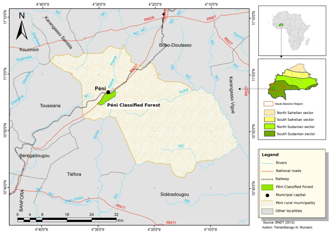
Figure 2.
Conceptual diagram of the relationships among landscape position, vegetation type, fire frequency, survey timing, woody species composition and estimated cover. The red arrow represents the association under study; it does not constitute causal evidence. The dashed arrow indicates that fire can modify vegetation type. Controlling for vegetation type may therefore remove part of the association related to fire history. The dotted arrow represents the possible effect of survey timing and phenology on the observed cover.
Figure 2.
Conceptual diagram of the relationships among landscape position, vegetation type, fire frequency, survey timing, woody species composition and estimated cover. The red arrow represents the association under study; it does not constitute causal evidence. The dashed arrow indicates that fire can modify vegetation type. Controlling for vegetation type may therefore remove part of the association related to fire history. The dotted arrow represents the possible effect of survey timing and phenology on the observed cover.
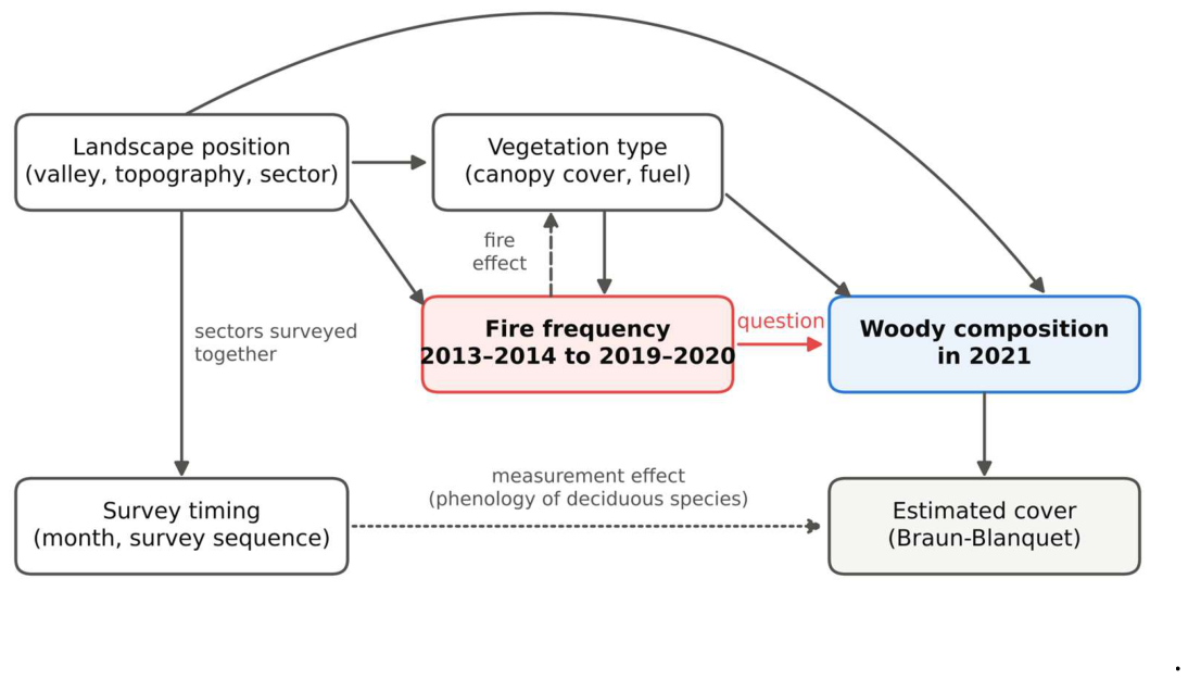
Figure 3.
Spatial distribution of the number of seasons detected as burned between 2013–2014 and 2019–2020 by the main Landsat model, for the 213 plots at Péni. Color indicates the number of burned seasons, from 0 to 7. Circles represent gallery forests, squares tree savannas, triangles shrub savannas and diamonds plantations. Detections characterize the surroundings of the plots within a radius of 30 m.
Figure 3.
Spatial distribution of the number of seasons detected as burned between 2013–2014 and 2019–2020 by the main Landsat model, for the 213 plots at Péni. Color indicates the number of burned seasons, from 0 to 7. Circles represent gallery forests, squares tree savannas, triangles shrub savannas and diamonds plantations. Detections characterize the surroundings of the plots within a radius of 30 m.
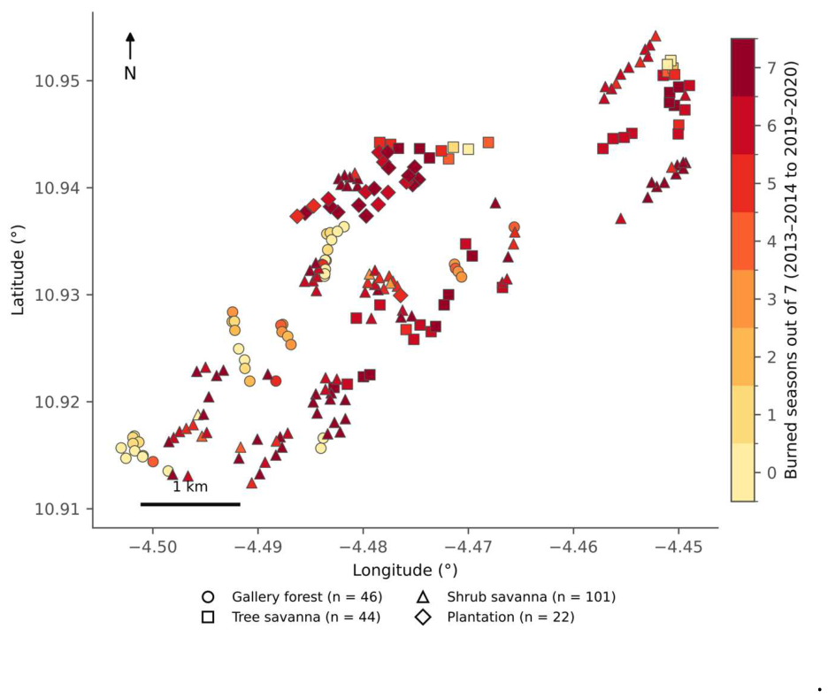
Figure 4.
Fire frequency by vegetation type. (a) Number of seasons detected as burned out of seven, from 2013–2014 to 2019–2020, with the main Landsat model. Each point represents a plot, jittered horizontally to limit overlap; the black bar indicates the mean. (b) Proportion of plots detected as burned per season from 2013–2014 to 2021–2022: Landsat as solid lines and Sentinel-2 as dotted lines. The shaded area covers the three calibration seasons, 2019–2020 to 2021–2022, for which Landsat predictions come from cross-validation. Colors denote the same vegetation types in both panels.
Figure 4.
Fire frequency by vegetation type. (a) Number of seasons detected as burned out of seven, from 2013–2014 to 2019–2020, with the main Landsat model. Each point represents a plot, jittered horizontally to limit overlap; the black bar indicates the mean. (b) Proportion of plots detected as burned per season from 2013–2014 to 2021–2022: Landsat as solid lines and Sentinel-2 as dotted lines. The shaded area covers the three calibration seasons, 2019–2020 to 2021–2022, for which Landsat predictions come from cross-validation. Colors denote the same vegetation types in both panels.
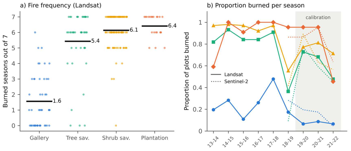
Figure 5.
NBR time series and fire detection dates for two plots: (a) shrub savanna plot cni146, with fire scars at survey; (b) gallery forest plot syg1, without fire scars at survey. Gray circles correspond to Landsat 7, dark gray squares to Landsat 8–9 and green dots to Sentinel-2. Sentinel-2 observations are shown before the removal of anomalous dates. Red dashed vertical lines indicate Landsat detections, purple dotted lines Sentinel-2 detections and the black line the survey date. The dates shown are detection dates, not the exact dates on which the fires occurred.
Figure 5.
NBR time series and fire detection dates for two plots: (a) shrub savanna plot cni146, with fire scars at survey; (b) gallery forest plot syg1, without fire scars at survey. Gray circles correspond to Landsat 7, dark gray squares to Landsat 8–9 and green dots to Sentinel-2. Sentinel-2 observations are shown before the removal of anomalous dates. Red dashed vertical lines indicate Landsat detections, purple dotted lines Sentinel-2 detections and the black line the survey date. The dates shown are detection dates, not the exact dates on which the fires occurred.
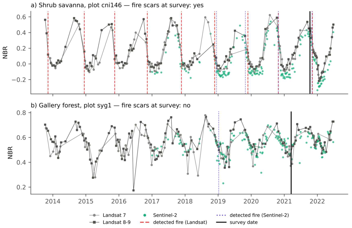
Figure 6.
Partitioning of the variation in woody species composition among fire frequency, vegetation type and the month–space set: (a) 213 plots; (b) 145 savanna plots, with savanna type as the vegetation type factor. Values are adjusted R2 expressed as percentages of total variation. Unique fractions correspond to each set after controlling for the other two; “∩” denotes a shared fraction that cannot be attributed to any one set. The residual fractions, not shown, are 56.10% and 62.94%, respectively. The horizontal scales differ between panels.
Figure 6.
Partitioning of the variation in woody species composition among fire frequency, vegetation type and the month–space set: (a) 213 plots; (b) 145 savanna plots, with savanna type as the vegetation type factor. Values are adjusted R2 expressed as percentages of total variation. Unique fractions correspond to each set after controlling for the other two; “∩” denotes a shared fraction that cannot be attributed to any one set. The residual fractions, not shown, are 56.10% and 62.94%, respectively. The horizontal scales differ between panels.
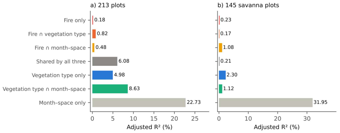
Table 1.
Plot characteristics by vegetation type. Woody species richness per plot: mean ± standard deviation; tree cover: median; burned seasons: mean ± standard deviation over seven seasons (Landsat, 2013–2014 to 2019–2020); late fires: fires detected from January to May/all burned seasons. Survey timing by vegetation type is given in Table S1.
Table 1.
Plot characteristics by vegetation type. Woody species richness per plot: mean ± standard deviation; tree cover: median; burned seasons: mean ± standard deviation over seven seasons (Landsat, 2013–2014 to 2019–2020); late fires: fires detected from January to May/all burned seasons. Survey timing by vegetation type is given in Table S1.
| Vegetation type | n | Woody species richness per plot | Tree cover (%) | Burned seasons (out of 7) | Late fires | Fire scars in 2021, n (%) |
| Gallery forest | 46 | 24.2 ± 6.5 | 70.0 | 1.6 ± 1.7 | 20/72 | 18 (39.1) |
| Tree savanna | 44 | 19.9 ± 6.8 | 7.5 | 5.4 ± 2.0 | 16/239 | 30 (68.2) |
| Shrub savanna | 101 | 12.9 ± 4.5 | 0.0 | 6.1 ± 1.1 | 42/620 | 101 (100.0) |
| Plantation | 22 | 11.0 ± 4.4 | 80.0 | 6.4 ± 0.7 | 19/141 | 22 (100.0) |
Table 2.
Agreement between fires detected during the 2020–2021 season before the visit date and fire scars recorded during the survey. TP: true positives; FP: false positives; FN: false negatives; TN: true negatives. In parentheses: 95% Wilson confidence interval. Specificity cannot be calculated where all plots showed fire scars.
Table 2.
Agreement between fires detected during the 2020–2021 season before the visit date and fire scars recorded during the survey. TP: true positives; FP: false positives; FN: false negatives; TN: true negatives. In parentheses: 95% Wilson confidence interval. Specificity cannot be calculated where all plots showed fire scars.
| Source | Plots | TP/FP/FN/TN | Recall (%) | Specificity (%) | Precision (%) |
| Landsat | All plots | 129/8/42/34 | 75 (68–81%) | 81 (67–90%) | 94 (89–97%) |
| Gallery forest | 2/2/16/26 | 11 (3–33%) | 93 (77–98%) | 50 (15–85%) | |
| Tree savanna | 24/6/6/8 | 80 (63–90%) | 57 (33–79%) | 80 (63–90%) | |
| Shrub savanna | 82/0/19/0 | 81 (72–88%) | – | 100 (96–100%) | |
| Plantation | 21/0/1/0 | 95 (78–99%) | – | 100 (84–100%) | |
| Sentinel-2 | All plots | 111/8/60/34 | 65 (57–72%) | 81 (67–90%) | 93 (87–97%) |
| Gallery forest | 4/4/14/24 | 22 (9–45%) | 86 (68–94%) | 50 (22–78%) | |
| Tree savanna | 22/4/8/10 | 73 (56–86%) | 71 (45–88%) | 85 (66–94%) | |
| Shrub savanna | 64/0/37/0 | 63 (54–72%) | – | 100 (94–100%) | |
| Plantation | 21/0/1/0 | 95 (78–99%) | – | 100 (84–100%) |
Table 3.
Unique contribution of fire frequency (Landsat, main measure) to woody species composition according to covariables, sample and response (adjusted R2, %; 9,999 permutations). Permutations are unrestricted for the row without covariables and restricted within months for the other rows. G: vegetation type (213 plots) or savanna type (savannas); Z: month, coordinates and retained dbMEM.
Table 3.
Unique contribution of fire frequency (Landsat, main measure) to woody species composition according to covariables, sample and response (adjusted R2, %; 9,999 permutations). Permutations are unrestricted for the row without covariables and restricted within months for the other rows. G: vegetation type (213 plots) or savanna type (savannas); Z: month, coordinates and retained dbMEM.
| Covariables | 213 plots | 145 savannas |
| None | 7.56 (< 0.001) | 1.70 (< 0.001) |
| G | 0.66 (< 0.001) | 1.31 (< 0.001) |
| G + coordinates | 0.48 (< 0.001) | 1.11 (< 0.001) |
| G + month | 0.50 (< 0.001) | 1.11 (< 0.001) |
| G + month + coordinates | 0.33 (0.002) | 0.70 (0.002) |
| Z | 1.00 (< 0.001) | 0.41 (0.012) |
| Z + G (main model) | 0.18 (0.014) | 0.23 (0.042) |
| Z (dbMEM selected with F) + G | 0.18 (0.015) | 0.23 (0.043) |
| Z + G, without plantations (191 plots) | 0.24 (0.008) | – |
| Z + G, presence–absence | 0.15 (0.012) | 0.19 (0.075) |
Table 5.
Slope of fire frequency (per burned season) on savanna plot attributes, after controlling for month, space and savanna type (Freedman–Lane, 9,999 permutations within months; q: Benjamini–Hochberg adjustment).
Table 5.
Slope of fire frequency (per burned season) on savanna plot attributes, after controlling for month, space and savanna type (Freedman–Lane, 9,999 permutations within months; q: Benjamini–Hochberg adjustment).
| Attribute | n | Slope | Standard error | Residual df | p | q |
| Woody species richness (species) | 145 | 0.558 | 0.334 | 123 | 0.120 | 0.301 |
| Tree cover (%) | 145 | 0.950 | 0.586 | 123 | 0.110 | 0.301 |
| Shrub cover (%) | 145 | 0.575 | 0.932 | 123 | 0.527 | 0.820 |
| Mean shrub height (m) | 145 | −0.014 | 0.058 | 123 | 0.820 | 0.820 |
| Mean tree height (m) | 44 | −0.071 | 0.164 | 23 | 0.676 | 0.820 |
Disclaimer/Publisher’s Note: The statements, opinions and data contained in all publications are solely those of the individual author(s) and contributor(s) and not of MDPI and/or the editor(s). MDPI and/or the editor(s) disclaim responsibility for any injury to people or property resulting from any ideas, methods, instructions or products referred to in the content. |
© 2026 by the authors. Licensee MDPI, Basel, Switzerland. This article is an open access article distributed under the terms and conditions of the Creative Commons Attribution (CC BY) license.
Copyright: This open access article is published under a Creative Commons CC BY 4.0 license, which permit the free download, distribution, and reuse, provided that the author and preprint are cited in any reuse.