
Submitted:
16 November 2026
Posted:
18 November 2026
You are already at the latest version
Abstract
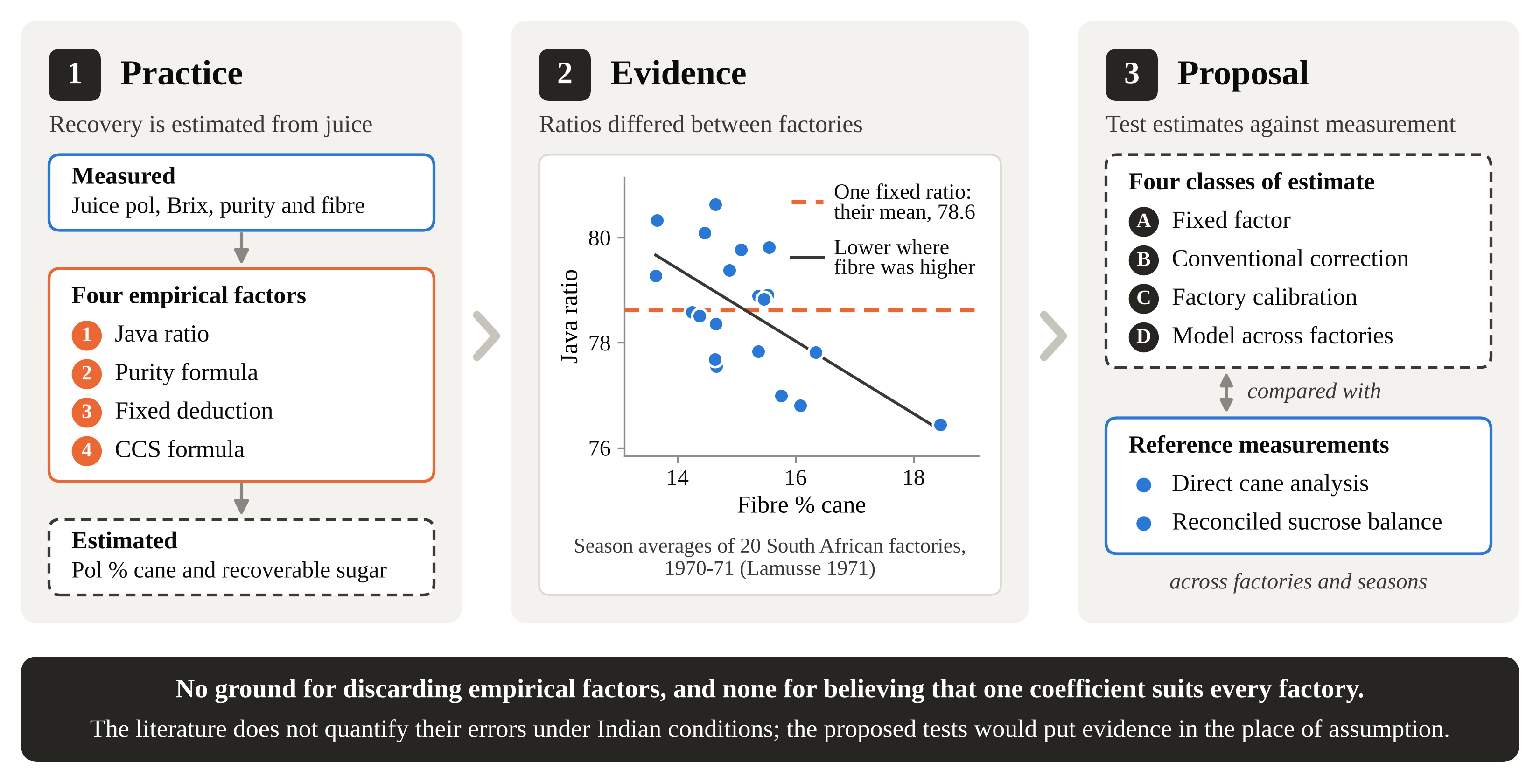
Sugar mills judge incoming cane and estimate recovery with polarimetry, refractometry, fibre determination and a few empirical conversion factors. This review examines four: the Java ratio, which converts the pol of first expressed juice to pol % cane; purity formulas for recoverable sugar; the commercial cane sugar (CCS) formula, which combines juice pol and Brix with fibre; and fixed deductions for factory losses. It asks how reliably each estimates cane quality and potential recovery when variety, fibre, maturity and factory practice change. The original literature shows that the limits were understood from the start: the factor was to be recalculated for each factory and period. Sensitivity calculations indicate the scale but describe the formulas, not measured errors. Published South African factory averages show ratios that differed between factories and tended to be lower where fibre was higher. The literature identified here does not provide enough independent evidence from several factories to quantify the errors of fixed factors under Indian conditions. The methods are compared by inputs, assumptions and biases. The proposed validation framework rests on direct cane analysis, reconciled sucrose balances and tests across factories and seasons.
Keywords:
sugarcane
; Java ratio
; pol % cane
; commercial cane sugar
; sugar recovery
; sucrose balance
; factory calibration
1. Introduction
Cane sugar manufacture was among the first agricultural industries to place its raw material and its process under routine chemical control. By the early twentieth century the Java industry had standard procedures for sampling cane, bagasse, juice and molasses, for weighing or calculating every stream, and for reporting the results each day and each period (Prinsen Geerligs 1917). The quantities it relied on, pol, Brix, fibre and purity, are the same ones that appear in the daily manufacturing report described for Indian factories today (Singh 2017).
What has changed less than might be expected is the set of shortcuts used to get from what is easy to measure to what a manager needs to know. A sample of first expressed juice is quick to take and to analyse. The sucrose content of the cane it came from is not, and the sugar that will finally be bagged is known only after milling, clarification and crystallisation are complete. Four kinds of empirical factor bridge these gaps. The first is a ratio that converts juice pol to cane pol. The second is a purity formula that converts sucrose in juice to recoverable sugar. The third is the commercial cane sugar (CCS) formula, which combines the pol and Brix of juice with the fibre of cane to give recoverable sugar. The fourth, found mainly in field and breeding studies, is a fixed deduction that converts cane pol to expected recovery. Each is convenient and each was calibrated under particular conditions of cane and factory. None of them measures the quantity it estimates.
These factors matter outside the laboratory because their outputs feed decisions. In India recovery is an important determinant of the cane price that the central government prescribes. The Fair and Remunerative Price (FRP) for 2026-27 is Rs 365 per quintal at a basic recovery of 10.25%. Rs 3.56 is added or removed for every 0.1 point of recovery, and no deduction is made below a recovery of 9.5% (CCEA 2026). Pricing also works under arrangements specific to states. Uttar Pradesh, Uttarakhand, Haryana and Punjab announce State Advised Prices (SAP), which are generally higher than the FRP and vary with the class of variety (Standing Committee 2023). The relation between measured recovery and the price actually paid for cane therefore differs between regions. The setting is a demanding one for any fixed coefficient. Indian factories stretch from the subtropical plains of Uttar Pradesh to the tropical Deccan, and the crop is planted in three seasons and stands for 10 to 18 months (NITI Aayog 2020). Cane is bought by weight, so the price a grower receives does not depend on the measured quality of the individual consignment. A factor tuned in one of these settings cannot be assumed to hold in another.
The question addressed here is how reliably the conventional empirical factors estimate cane quality and potential recovery, and how that reliability should be tested. Three subsidiary questions follow from it.
- How did the conventional methods for measuring cane quality and estimating recoverable sugar develop, and what did their originators say about their limits?
- How sensitive are the estimates to the assumptions built into each factor, and what is known about the errors that arise when a fixed factor is applied across different cane and factory conditions?
- What measurements and comparisons would show whether a fixed factor, a conventional correction or a calibration specific to one factory is accurate enough for its purpose?
The review does not set out to show that conventional factors are wrong. Its position is that they rest on identifiable assumptions and that their predictive validity across factories and seasons is an empirical matter which independent measurements have yet to settle. Sections 3 to 6 trace the methods and examine each factor in turn, Section 7 compares them and Section 8 proposes a validation framework. The Indian setting in detail, the planning of cane supply and forecasts made from field and satellite data are outside the scope of this review.
2. Scope and Approach
This article is a critical narrative review with a proposed validation framework. It draws on four groups of sources. The first is the historical technical literature on chemical control, chiefly Prinsen Geerligs (1917, 1924) on Java practice and Kelly (1974) on quality control and cane payment. The second is the body of methods and standards that define how cane is analysed and paid for: the Australian laboratory manual (BSES 1984), the World Bank study of cane payment systems (LMC International 1997), the Indian audit guide for the industry (ICAI 2010), Method GS5-2 of the International Commission for Uniform Methods of Sugar Analysis, ICUMSA (ICUMSA 2024), and a practitioner’s account of laboratory control in an Indian factory group (Singh 2017). The third is official Indian material on pricing and on the definition of recovery: the report of the parliamentary Standing Committee (2023), which records the evidence of the Department of Food and Public Distribution (DFPD), the guidelines of that department on sugar streams diverted to ethanol (DFPD 2023) and the announcement of the cane price for 2026-27 (CCEA 2026). The fourth is published evidence from industries that have recorded these quantities over many years. It is drawn mainly from the Proceedings of the South African Sugar Technologists’ Association and supplemented by work from Australia, Brazil, Cuba, Mozambique and Zimbabwe.
The author’s working collection of historical texts, official reports and practitioner material formed the starting point. Targeted searches were then run in November 2026 on the open web, on publisher platforms (SpringerLink, ScienceDirect, Frontiers, MDPI, ACS Publications and PubMed Central), in the document repositories of the United Nations Industrial Development Organization (UNIDO) and the World Bank, on the website of ICUMSA and in the open archive of the South African Sugar Technologists’ Association. The searches combined sugarcane with the terms Java ratio, pol % cane, commercial cane sugar, cane payment, sugar recovery, direct analysis of cane, undetermined loss and measurement uncertainty. A source was retained if it reported measured cane quality or recovery or documented a method or a practice at first hand, and primary documents were preferred to secondary accounts. One reviewer made the selection. Generative AI tools were used to run the searches, to extract and summarise the content of sources, to check statements in the text against them and to prepare drafts, calculations and figures. The author reviewed that output and is responsible for the choice of sources and for what is said about them. No subscription bibliographic database was searched and no formal scoring of study quality was applied.
Recovery, used without qualification, means sugar produced as a percentage of cane crushed, and the sugar season runs from October to September. Simple calculations are used in several places to show the size of an effect, and the inputs are stated each time. Five limits apply. This is not a systematic review, and no claim is made that every relevant study was found or screened. Statements about practice in Indian mills rest on the guidance documents and reports cited. They describe documented practice and may not describe every mill. The calculations in Section 5 and Section 6 are theoretical sensitivity analyses. They show how an estimate responds to an assumption and are not measurements of error in any factory. The measurements summarised in Section 5.4 come from other countries and other periods. They show what was observed where the comparison was made and are not evidence about Indian factories. The framework in Section 8 is a proposal and has not been tested here.
3. Historical Evolution of Cane Quality Assessment
3.1. Chemical Control in the Java Industry
The handbook that Prinsen Geerligs revised in 1916 described how each product of the factory should be sampled and analysed and how the results should be brought together (Prinsen Geerligs 1917). Three features of that system deserve to be recalled, because later practice kept the arithmetic and lost some of the caution.
The first is that the composition of cane was never measured on the cane. Prinsen Geerligs thought it close to impossible to sample a day’s crushing accurately, given the differences between varieties, fields, stalks and even the parts of a single stalk. Sucrose in cane was therefore obtained as the sum of sucrose in raw juice and sucrose lost in bagasse, divided by the weight of cane. Fibre in cane was obtained from the fibre found in bagasse. Both figures were reliable only over a period long enough for all the weighed cane to have been crushed.
The second is that the factor linking juice to cane was presented as an expedient. For its daily report the factory needed a quick estimate, and it got one by multiplying the sucrose content of first mill juice by a factor. Prinsen Geerligs explained why no exact factor could exist. If cane were a uniform juice held in dry fibre, the factor would be (100 minus fibre) divided by 100. In reality fibre holds water of its own, the cells differ in hardness and in the richness of their juice, and the first juice expressed is always the richest. He recorded that many factors based on fibre had been proposed and that none was accurate. His advice was to take the simplest one and to remember that its value was not absolute. The factor for each period was to be calculated from the real figures of the period before. Only at the start of a season, with nothing to go on, were default values used: 0.85 for soft cane and 0.80 for hard cane. The original Java factor was therefore specific to a factory, updated through the season and dependent on the type of cane.
The third is that the system already linked the field to the factory. Plots were sampled through the ripening period and cut when polarisation and purity stopped rising. Cane arriving at the factory was heaped by field, each heap was crushed separately once a day, and the first mill juice was analysed so that the sugar expected from each field could be estimated. Prinsen Geerligs was explicit that such estimates were only comparable with one another. At the end of the season they were to be scaled by the ratio of sugar made to sugar calculated.
The same book gives the formula, usually credited to Winter, for the raw sugar of 96 polarisation to be expected from raw juice:
It comes with the warning that the values are approximate and shift with the purity to which the final molasses is exhausted. The picture is of an industry that calibrated its rules of thumb continuously against its own weighed and analysed production.
3.2. Cane Payment and the Australian Formula
A second line of development came from the need to pay growers. Kelly (1974), writing for a UNIDO meeting on sugar processing equipment, set out the options as they stood fifty years ago. Payment on weight alone was the simplest. In his assessment it gave the farmer no reason to grow better cane, to deliver it fresh or to keep it clean. The Java ratio offered an easy route from first expressed juice to pol in cane, but it made no allowance for fibre and lost its usefulness when fibre varied appreciably. The Australian CCS formula went further. It corrected both pol and Brix for fibre and deducted an allowance for impurities. Kelly regarded it as imperfect and still worth keeping, partly because the impurity term rewards cleaner and riper cane. He also described the direct analysis of shredded cane practised in South Africa and the core sampler and hydraulic press procedure associated with Hugot, in which a weighed sample is pressed under fixed conditions and the juice and press cake are analysed.
The World Bank study by LMC International (1997) surveyed how these methods were used for payment across the main cane industries. Most paid on quality through an empirical formula built on sucrose, fibre and juice purity. Australia, Jamaica, Mauritius, South Africa and Thailand paid each grower on the grower’s own cane, while Argentina and Mexico paid on the mill average. Fiji and northern India paid on weight. The study pointed to weaknesses in first expressed juice sampling. It cannot be used where cane is washed or where diffusers replace mills, and the setting of the mill rolls may bias the result.
3.3. Standard Methods
Standardisation completed the picture. The Australian laboratory manual fixed the measurements and calculations for mill laboratories (BSES 1984), and ICUMSA maintains reference methods for cane as it does for sugar. Method GS5-2, issued in 2024 with official status, determines polarimetric sucrose, dry substance and fibre in cane prepared with a hydraulic press and is intended for cane payment (ICUMSA 2024). The laboratory guidance documented for Indian mills belongs to the same family of methods. Singh (2017) lists the ICUMSA subject groups, the Bureau of Indian Standards specifications for plantation white, refined and raw sugar, and the elements of good laboratory practice that make results comparable between shifts and factories.
Two conclusions follow for anything built on these data. Good reference measurements already exist and should anchor any new model. No statistical method can repair reference data that are inconsistent or biased at source.
4. Measurement Fundamentals
4.1. Pol, Brix and Purity
Pol is the apparent sucrose content read from a polarimeter. It is an operational quantity. Reducing sugars rotate polarised light in the opposite sense to sucrose, so pol usually sits slightly below true sucrose, and Prinsen Geerligs (1917) recommended double polarisation wherever accuracy mattered. Dextran, which forms in stale cane (Solomon 2009), is strongly dextrorotatory and pushes the reading the other way. This is one reason deteriorated cane can look better in the laboratory than it performs in the factory.
Brix is the percentage of dissolved solids as indicated by a refractometer or hydrometer. Apparent purity is the ratio of the two:
Apparent purity is an index formed from two operational measurements. It indicates roughly what share of the dissolved material is sucrose. It is not an exact chemical proportion, because pol is not true sucrose and Brix is not true dry substance. Nor does it say how much juice the cane holds, so two consignments of equal purity can carry very different amounts of sugar per tonne.
4.2. Cane Pol and Juice Pol
Pol % cane is expressed on the mass of cane, and pol % juice on the mass of the juice analysed. They differ because cane contains fibre and because the juice sampled is not the average juice of the stalk. Three juices have to be kept apart. First expressed juice, from the first mill or a laboratory press, is the richest. Mixed juice is the whole juice sent to process, diluted by imbibition water. The third is the extract obtained from prepared cane by wet disintegration or pressing. A conversion factor derived for one of them cannot be applied to another without validation.
Figure 1 sets these quantities out in two rows. The lower row is the chain that a factory measures or infers in routine control, and it ends in actual recovery. The upper row holds the estimates that the empirical formulas of Section 5 and Section 6 produce, together with the measurements that each formula needs: the pol and Brix of first expressed juice, fibre % cane, or the pol and purity of mixed juice. An estimate of recoverable sugar is a different quantity from sugar actually recovered, and the figure keeps the two apart.
Indian factory control guidance obtains the pol of cane by the inferential method inherited from Java. Juice and added water are weighed or metered, bagasse is found by difference, and
Fibre % cane is derived from bagasse in the same way. The Java ratio is then calculated from the result and reported beside it (Singh 2017). The distinction matters. Used like this, the ratio is an output of the mass balance, averaged over a day or a period, and it serves as a check on milling and on the analysis. It becomes an assumption only when it is turned round and used to predict the pol of cane that has not yet been milled, such as a field sample, a single cartload or the supply expected next month.
Table 1 lists the guide values that Singh (2017) gives for an Indian plantation white sugar factory.
4.3. Recovery: Actual, Expected and Deemed
Actual recovery is
with both quantities taken over the same period and corrected for sugar still in process. Three other quantities are often called recovery and should not be confused with it. Expected recovery is what the boiling house should deliver from the juice it receives, calculated from juice purity. Deemed recovery is an accounting figure used when part of the sugar stream goes to ethanol. Estimates made from the pol of field or laboratory samples form a further category and are taken up in Section 6.
For pricing purposes the DFPD defines the recovery rate as the sugar actually bagged plus the sugar sacrificed for ethanol, divided by the cane crushed. Where sugar is diverted to ethanol it gives this formula for the estimated recovery (Standing Committee 2023):
Here J is the purity of mixed juice and K is 1.002 for plantation white sugar. The expression is the SJM formula of boiling house control (Hugot 1986; Rein 2007),
with the sugar purity S set to 100 and the molasses purity M set to 35.6, since 100 minus 35.6 is 64.4. The constant is therefore a convention for the purity to which final molasses is exhausted, and the formula allows for no other loss between mixed juice and sugar. With pol in mixed juice at 12.5% of cane and a purity of 82 it returns a recovery of 11.0%.
The guidelines that the DFPD issued on 21 December 2023 for factories and distilleries producing ethanol, in place of its earlier guidance, state where the formula applies (DFPD 2023). It is the estimate of recovery given for factories that divert B heavy molasses in place of final molasses, and for those that divert the whole of their juice or syrup. Where only part of the juice or syrup is diverted, recovery is to be calculated from the quantity diverted and the actual purity of the final molasses obtained. The fixed constant is thus a convention for particular cases of diversion. It is not offered as a description of every boiling house, and under partial diversion the official method itself calls for the molasses purity that the factory achieves.
Table 2 shows how the factor moves with juice purity and sets it beside the Winter factor of Section 3.1. Under the official formula one point of purity is worth about 0.8 points of boiling house recovery. The two columns have the same algebraic form. The Winter factor 1.4 − 40/J is identical to the SJM expression with S at 100 and with 28.57 in the place of M. That number is an equivalent parameter under a convention of sugar of 100 pol. It is not a molasses purity that the users of the Winter formula assumed or measured, and the formula was stated for raw sugar on a basis of 96 polarisation. The identity shows only that the two formulas respond to juice purity in the same way, and why the Winter factor is the larger of the two at every juice purity in the table.
The practical consequence is that a forecasting system has to state which of these quantities it predicts. A model trained on bagged sugar per tonne of cane will show a fall after 2018-19 for the simple reason that more sucrose left the factories as ethanol. The sugar diverted rose from about 0.3 million tonnes in that season to about 3.5 million tonnes in 2021-22 (Standing Committee 2023).
5. The Java Ratio: Basis and Limits
5.1. Definition
The Java ratio is the pol of cane expressed as a percentage of the pol of first expressed juice (ICAI 2010; Singh 2017):
Writing j for the ratio as a decimal fraction,
Singh (2017) gives 80 ± 2 as the value to expect in a well run north Indian factory. Prinsen Geerligs (1917) worked an example with 80.9 and suggested 0.85 and 0.80 as opening values for soft and hard cane. These numbers describe averages over the whole supply of a factory. None of the sources presents them as constants.
5.2. Theoretical Sensitivity to the Coefficient
What follows is a sensitivity analysis. It shows how far an estimate moves when an assumed coefficient moves, and it does not measure how wrong the coefficient is in any factory. A first expressed juice of 15% pol gives 12.0% pol in cane with a coefficient of 0.80, the centre of the range that Singh (2017) gives, and 10.8% with a coefficient of 0.72. The lower value is an illustration chosen for this review. None of the sources consulted documents it as a coefficient in industrial use, and the lowest of the South African season averages examined in Section 5.4 was 0.76. The difference of 1.2 points comes entirely from the choice of coefficient. Inside the narrower band of 0.78 to 0.82 that Singh treats as normal, the estimate for the same juice still ranges from 11.7% to 12.3%. If about 84% of the pol in cane is recovered (Section 6.3), that spread of 0.6 points in estimated cane pol corresponds to about 0.5 points in the estimate of recovery. A different coefficient changes the estimate and leaves the sugar in the cane where it was. How large the actual error is at a given factory depends on how far its true ratio departs from the value assumed, and the literature identified for this review contains no distribution of the ratio across Indian factories, varieties or periods. Section 5.4 summarises what has been published elsewhere. Supplying the distribution for Indian conditions is the first purpose of the design in Section 8.
5.3. Fibre, Variety and Sampling
Why should the coefficient move at all? The simplest physical model, already written down by Prinsen Geerligs, treats cane as fibre plus a juice of uniform composition and gives j = (100 − F)/100, where F is fibre % cane. The Australian CCS convention subtracts a further five units to allow for the water held by fibre and for the richness of first expressed juice compared with the rest (Kelly 1974; LMC International 1997):
Under either form each unit of fibre lowers the coefficient by 0.01. That slope follows from the algebra of the two conventions and is not an empirical finding. Figure 2 plots both against the guide band of 0.78 to 0.82. The Australian form returns 0.80 at 15% fibre and 0.815 at the 13.5% fibre that Singh regards as typical, so the Indian guide value and the Australian convention agree with each other. The same arithmetic shows how narrow the conditions for a constant coefficient would be if the convention held. Across a fibre range of 12 to 17%, which is not unusual between varieties, ratoons and harvest conditions, the implied coefficient runs from 0.83 to 0.78. For a juice of 16% pol the estimated pol of cane then runs from 13.3% to 12.5%, and one unit of fibre moves the estimate by 0.16 points. Whether the ratio observed in Indian factories follows fibre with this slope, a steeper one or none at all was not reported in the literature identified, and it is one of the questions that the comparison in Section 8 is meant to answer. The one set of published factory averages examined here shows a slope of the same sign and of similar size, on a somewhat different analytical basis (Section 5.4).
Fibre is only the most tractable influence. Trash, tops and soil delivered with the cane raise the fibre of what is milled without changing the stalk (Prinsen Geerligs 1917), and Imbachi Ordonez et al. (2025) had to deal with cane carrying large amounts of soil, leaves, roots and tops in Louisiana factories. Variety and maturity change the distribution of sugar along the stalk. Nawi et al. (2013) measured Brix values from 7.6 to 22.2 across the internodes of three Australian varieties, with a steady decline along the stalk, so the juice expressed first depends on how the stalk is topped and prepared. Mill settings affect which cells give up their juice at the first rolls (LMC International 1997).
Sampling adds a separate problem. A ratio calculated from the aggregated production of a factory is an average over all the cane crushed in the period. Applied to one consignment it will be biased whenever that consignment differs from the average in fibre, cleanliness or maturity, and these are exactly the consignments a planner most wants to identify.
There is also a risk of circular calibration. If the coefficient is tuned so that predicted recovery matches what the factory achieved last season, any error in the assumed factory losses is absorbed into the coefficient. The two relationships, juice to cane and cane to sugar, need to be estimated and validated separately.
5.4. Published Evidence on the Ratio in Practice
The calculations above describe formulas. Measurements of how the ratio behaves were published by industries that used it for payment, and the South African record is the fullest found for this review. In the 1950s South African cane was paid for on a sucrose content obtained by applying the weekly Java ratio of the mill, calculated from the whole crush of the week, to the first expressed juice of each consignment. Antonowitz (1957) examined the method and concluded that a common ratio places a premium on dirty cane and on cane of high fibre, at the expense of growers who deliver clean cane of low fibre. Among the influences on the ratio of a single consignment he listed topping, fibre, trashing, the cleanliness of the cane, rain, maturity and the performance of the mills. He cited earlier tests from the same industry in which no result was out by more than 1.6 units of sucrose % cane, which at 14% sucrose is about 11% of the value. In the discussion that followed, the meeting accepted that the ratio was not the best method but had no better one to put in its place, and the determination of fibre was named as the central difficulty.
Factory averages point the same way. Table B of the annual summary of laboratory reports for the 1970-71 season gives the sucrose % cane, the fibre % cane and the Java ratio that each factory reported in its final laboratory report (Lamusse 1971, pp. 10 and 11). The figures of the source show how its ratio is formed: the sucrose % cane is divided by the pol of first expressed juice, which is the product of the Brix and the apparent purity of that juice (Appendix A). The ratio of Section 5.1 has pol in both terms, so the two are not strictly the same quantity. They coincide only where the sucrose and the pol of cane are equal, which need not hold when other optically active substances are present (Section 4.1). The values for the twenty South African factories, and for five other Southern African factories in the same table, are reproduced in Appendix A (Table A1), where eighteen of the twenty printed ratios are also shown to be reproduced by recalculation from other figures of the same source. Among the South African factories the ratio ran from 76.4 to 80.6, with an unweighted mean of 78.6 and a standard deviation of 1.2, and fibre ran from 13.6 to 18.5%. The factory with the most fibre had the lowest ratio. A least squares line fitted to the twenty pairs for this review has a slope of −0.69 units of the ratio per unit of fibre, with a standard error of 0.21 and a 95% confidence interval from −1.13 to −0.25, and the correlation coefficient is −0.62 (Figure 2a; Table A2). The interval contains the −1.0 that the fibre conventions imply, and fibre accounts for about 38% of the variance between factories. The factory of highest fibre has far more leverage on the line than any other. Without it the slope is −0.73, with a 95% confidence interval from −1.39 to −0.06, and the correlation coefficient is −0.49. The slope changes little when the two ratios that are not reproduced by recalculation are left out or recalculated. With the recalculated ratios and without the factory of highest fibre, however, the interval runs from −1.30 to 0.06 and includes zero (Table A2). The association is therefore consistent in sign across these cases, but its strength leans on the range of fibre that one factory supplies. The allowance that each average implies, 100 − F less the ratio, ranged from 4.6 to 7.8 units and averaged 6.2, against the 5 units of the Australian convention. A single ratio set at the mean of the twenty, applied to juice of 16% pol, would have produced estimates of cane pol differing by up to 0.35 units from those made with each factory’s own seasonal ratio. That figure is a difference between two estimates made with coefficients. It is not an error measured against direct analysis of cane, which these reports do not contain.
Four cautions apply. The comparison with the fibre conventions is indicative. The observed ratios rest on sucrose in cane and pol in juice, the conventions on pol in both, and the regression shows an association in the expected direction. It does not validate the 5 unit allowance of the Australian convention or the predictive value of any fibre factor. These are season averages for whole factories, from one year in one industry, and they say nothing about single consignments. The summary reproduces what the factories reported and does not say how each obtained its fibre and the sucrose of its cane. If both came from the factory balance, as was usual in chemical control, their errors are shared. Finally, twenty points give the slope little precision, as the width of the interval shows.
Direct analysis later removed the need for the ratio in payment. South African consignments have since been sampled across the full width of the stream of shredded cane and analysed directly for pol, Brix, moisture and fibre (Schäffler et al. 2003). Work done when the press method was assessed against direct analysis bears on the ratio as well. Brokensha et al. (1976) analysed 104 samples by both methods and found that the ratio of the pol of the absolute juice of cane to the pol of press juice fell as fibre rose, with a correlation coefficient of −0.69. The relation differed between varieties, and for one variety there was none (r = −0.18 in 22 samples). Soil in the sample caused the fibre estimated from the mass of press cake to be understated by 2.6 units. Even under laboratory control, then, the relation between expressed juice and cane was neither constant nor the same for all cane.
Extraneous matter is the other influence that has been measured. In Brazilian trials known amounts of leaves, tops and straw were added to clean stalks (Madaleno et al. 2026). Each 1% added raised the fibre of the cane by 0.15 to 0.18 units, depending on the method by which fibre was determined, and 12% lowered the pol of the cane by 7.7% of its value. The authors judged the estimate of fibre from the mass of wet press cake, which Brazilian mills use in routine analysis, to be unsuited to green cane. A review of work on processing trash with the cane concluded that it significantly reduces sugar recovery and sugar quality (Kent 2014).
None of this is evidence about Indian factories. It shows that where the ratio has been set beside fibre or beside direct analysis it has varied between factories, varieties and consignments in the direction that the fibre conventions predict, and by amounts that matter for payment. It also shows that the comparison can be made with figures that factories already record. The literature identified for this review contains no equivalent for India.
5.5. A Conditional Coefficient
A more defensible position is to treat the coefficient as conditional:
where F is fibre, V stands for variety, M for maturity and S for sampling and site conditions. This is a hypothesis to be tested. It is also close to what Prinsen Geerligs prescribed when he asked for a factor by type of cane, recalculated each period. Two outcomes are possible and both would be useful. Variety, maturity and site may explain variation that fibre does not, in which case a calibrated model is justified. Or a simple fibre adjustment may do as well as anything more elaborate, in which case the industry already has the tool and needs only routine fibre data. Model comparisons should be designed so that the second outcome can be detected (Section 8).
6. Commercial Cane Sugar and Empirical Recovery Deductions
6.1. The Fibre Adjusted CCS Formula
The Australian formula estimates the sugar that a mill of standard efficiency should recover from cane. In its usual form (Kelly 1974; BSES 1984)
where the pol and Brix of cane are obtained from first expressed juice and fibre:
Pj and Bj are the pol and Brix of first expressed juice and F is fibre % cane. The formula rests on one empirical assumption, that each unit of soluble impurity carries half a unit of sucrose into molasses (Kelly 1974). The two fibre allowances, known as the 3 and 5 factors, are still the Australian means of deriving the Brix and pol of cane from first expressed juice (Wright 2005).
A juice of 16% pol and 19% Brix, which is a purity of 84.2, from cane of 14% fibre gives a pol in cane of 12.96, a Brix in cane of 15.77 and a CCS of 11.56. Raising fibre to 16% lowers CCS to 11.27, and lowering it to 12% raises CCS to 11.84 (Table 3). The formula thus carries both corrections that the Java ratio lacks, one for fibre and one for purity.
CCS is still an estimate made under stated assumptions. LMC International (1997) recorded that Australian cane quality declined from the 1960s to the late 1980s while the formula remained in use. Bramley et al. (2012) later drew attention to the variation of CCS within a single block, which means that even a sound formula returns different answers depending on where in the field the sample was cut. CCS should not be read as the recovery that a given factory will achieve.
6.2. The Fixed Deduction
Field experiments and breeding trials often need a recovery figure without access to a factory. A common device is to subtract a constant from the pol reading. Mehdi et al. (2023), in a pot study of two Pakistani varieties under heat stress, reported recovery in this way with an allowance of 2.5 for operating losses in the mill, and they stated that the loss varies from mill to mill. Written out,
The device is reasonable for ranking treatments inside one experiment. It should not be carried over to factory forecasting. Its use in one study is no evidence that Indian mills apply it, or that 2.5 is the right allowance anywhere.
6.3. What a Sucrose Balance Says About the Deduction
The sugar that fails to reach the bag is lost in identifiable places. Some leaves in bagasse, some in filter cake and some in final molasses. The remainder, made up of inversion, spillage and measurement error, is reported as undetermined loss. Kelly (1974) pointed out that this last item collects the errors of every other measurement and can even appear as a gain.
Singh (2017) gives an illustrative balance for an Indian factory. Of 100 units of sucrose in cane, 95 reach mixed juice, 4 leave in bagasse and 1 is lost at the mills. Of 100 units in juice, 88 are recovered as sugar, 10 go to final molasses, 0.5 to filter cake and 1.5 to handling and chemical losses. Chaining the two stages gives 83.6 units in sugar for every 100 in cane (Figure 3). Final molasses takes 9.5 units. It is the largest single loss and the one most sensitive to juice purity (Table 2).
On this balance cane of 13% pol yields 10.9% of cane as pol in sugar, and the total loss is 2.1 points of cane. A fixed deduction of 2.5 gives 10.5%. The two rules behave differently as cane quality changes (Figure 4). A proportional loss takes fewer points from poor cane and more from rich cane. A fixed deduction takes the same 2.5 points from cane of 11% pol, where it implies an overall recovery of 77%, as from cane of 15% pol, where it implies 83%. Real factories fit neither rule exactly, because poor cane usually has lower purity and so loses a larger share of its sucrose to molasses. This is the behaviour that matters most for planning, and only a balance that carries purity can represent it.
6.4. Separating Cane Quality from Factory Efficiency
The balance can be written compactly as
where Pc is pol % cane, E is the fraction of the pol in cane that enters mixed juice (mill extraction), B is the fraction of the pol in mixed juice recovered in sugar (boiling house recovery) and qs is the pol of the sugar produced, expressed as a fraction. With Pc at 13, E at 0.95 and B at 0.88 the pol recovered in sugar is 10.87% of cane, which is the quantity plotted in Figure 4. Dividing by a sugar pol of 0.998 gives 10.89% of cane as sugar, and both figures round to 10.9%. The product of E and B is the overall recovery of factory control (Wienese 2003). This is a simplified representation and not a regulatory formula. Its value lies in keeping three things apart: what the field delivered, what the mills extracted and what the boiling house recovered. Each responds to different decisions. Variety, harvest age and cut to crush delay act on Pc and on purity. Cane preparation, imbibition and mill settings act on E. Purity, clarification and molasses exhaustion act on B. A model that predicts cane pol well cannot be assumed to predict recovery well, and a fall in recovery cannot be assigned to the field or to the factory without the intermediate figures.
6.5. Formulas with Recalculated Factors
Some payment formulas build the recalculation in. The estimated recoverable crystal (ERC) of the Zimbabwe industry is a linear function of the composition of cane determined by direct analysis (Mutatu 2023):
Here P, N and F are the pol, non pol (Brix less pol) and fibre % cane. The factor a is the fraction of the pol in cane that is accounted for in sugar, bagasse and final molasses, b is the pol lost in molasses per unit of non pol, and c is the pol lost in bagasse per unit of fibre. The factors are not constants. Provisional values, the averages of the two preceding seasons, are used while the crop is crushed. Actual values are calculated when the products of the season have been reconciled, and the payments to growers are adjusted. Recalculation of the same kind is found in South African factory control, where one factory has valued a stream returned from its refinery with the SJM formula at the actual purity of its molasses and not at a conventional one (Wienese 2003). In both cases the form of the formula is kept and its constants are derived again from the results of the factories to which it is applied. That is the practice Prinsen Geerligs asked for.
7. Comparison of the Empirical Methods
Table 4 brings the methods of Sections 3 to 6 together. For each it lists what is measured, what is estimated, the assumptions on which the estimate rests, the bias that is known or to be expected, and the conditions under which the method should be recalibrated. Direct cane analysis is included as the reference against which estimates of cane pol have to be judged.
Three points stand out. The first is that the methods do not estimate the same thing. The Java ratio and its fibre based variants give pol % cane. The purity formulas, the CCS formula, the ERC formula and the fixed deduction give recoverable sugar under stated conventions. Only a sucrose balance over a crushing period gives the recovery that a factory achieved (Section 6.3). Agreement or disagreement between estimates of different quantities says nothing about the accuracy of either. Nor are the figures of one kind. Direct analysis is an analytical determination made on a sample by a reference method. Pol % cane by the inferential method is a factory figure, assembled from streams that are weighed and analysed, and it holds for the period over which they were totalled. The remaining entries are estimates made by formula. A study that mixes the three without saying so cannot be interpreted.
The second is that every assumption in the table can be checked with determinations that a factory laboratory already makes or is able to make. Fibre, the purity of final molasses and the pol of bagasse are routine. None of the methods has to be taken on trust.
The third is that the evidence on bias is thin and comes from elsewhere. The sources state the direction in which an estimate should move and the conditions under which it does so, and the algebra gives the size of the movement if a convention holds. The measurements summarised in Section 5.4 are consistent with that direction for the Java ratio in one industry. The targeted search made for this review found no published comparison of these estimates with direct cane analysis across Indian factories, varieties and seasons. Section 8 describes the comparison that would supply one.
8. A Validation Framework for Conventional Factors
The working hypothesis is modest. It is that calibrated, physically consistent estimates predict cane pol and recovery better than fixed universal factors under some conditions. How much better, and under which conditions, is an empirical matter. The framework below is meant to settle it in a way that a sceptical chief chemist would accept.
8.1. Targets and Model Classes
The comparison has to be organised around the quantity being predicted, because the methods in use do not all aim at the same one. A model can be judged only against others that predict the same target on the same samples. Two evaluations are therefore kept apart (Table 5). The first concerns the pol % cane of a sample or consignment, with direct cane analysis as the reference. The second is an in process forecast of the recovery of a factory over a defined crushing period, made after the juice of the period has been analysed and before its outcome is known. Its primary reference is actual recovery, which is sugar weighed and corrected for stock in process, divided by cane weighed (Section 8.2). In each evaluation four classes of model, ordered by complexity, are fitted and tested on identical samples or periods, and the first two classes are the baselines that anything more elaborate has to beat. CCS enters the second evaluation only as a predictor or as a benchmark estimate. It is never the target.
Each evaluation also fixes the moment at which the estimate is made, so that all classes draw on the same information (first row of Table 5). In the first evaluation the estimate is made when the first expressed juice of the sample has been analysed, together with its fibre where a model uses fibre. The direct analysis of the same sample is withheld until the estimates are fixed. The second evaluation is defined as an in process forecast of recovery. It is issued for a crushing period after the laboratory analyses of first expressed juice, mixed juice and bagasse for that period are available, and before the outcome is known, that is, before the sugar of the period has been bagged and the stock in process reconciled. Neither the Java ratio nor a purity formula can be applied earlier than that, because each needs juice from cane that has already been crushed. A model may use any measurement that exists at that moment, and the records of earlier periods. It may not use the sugar bagged, the stock in process or the final molasses of the period it predicts. The classes then differ in the calibration they carry and not in what they are allowed to see.
Each evaluation should report whether each step up in complexity produces a meaningful gain over classes A and B on its own target. The study should count as successful even if the answer for some steps is no. Prediction before harvest is a distinct task with a different information set. Models for it, which add field, weather, satellite and logistics variables, belong to neither evaluation and are outside the scope of this review. The two evaluations are linked only at the end, when the best predictor of cane pol from the first is used as an input to the second and its contribution to the error in recovery is measured.
8.2. Reference Measurements
Each evaluation needs its own reference. For the first, cane pol has to be determined directly on the cane. The hydraulic press method of ICUMSA GS5-2 or wet disintegration can be used, on samples drawn by a core sampler or from the stream of shredded cane (ICUMSA 2024). Each reference sample should be paired with the pol and Brix of first expressed juice, fibre, variety, crop class, age, plot, time of cutting and time of sampling. Values predicted by near infrared (NIR) spectroscopy are model outputs and belong among the predictors, never in the reference set.
A reference value has an uncertainty of its own. That uncertainty limits how confidently small differences in predictive performance can be resolved, and it should be carried into the evaluation of the models. In the South African cane testing laboratories the standard deviations of duplicate subsamples analysed directly were 0.3 units for pol and for Brix and 1.5 units for fibre, and an earlier estimate had put the error of sampling and analysis together at 0.4 units of pol. Predictions by NIR on an independent set of 371 consignments had standard errors of 0.5 units for pol and 0.9 for fibre (Schäffler et al. 2003). Two consequences follow. The first is that reference analyses should be duplicated on a share of the samples, so that the repeatability of the reference is known for the laboratories taking part and can enter the comparison, through replicate means or through a model that allows for error in the reference. The second is that fibre, the least precise of the determinations, is an input of every fibre adjusted formula. A difference of 1.5 units of fibre moves the coefficient of the CCS convention by 0.015 and the estimate of cane pol by 0.24 units at a juice pol of 16%. Part of the error of a fibre adjusted estimate will therefore be error in the fibre figure and not in the formula.
For the second evaluation the primary reference is actual recovery over the period, that is, sugar bagged, corrected for the change in stock in process, divided by cane crushed. Sugar bagged and cane crushed are weighed. The correction for stock in process is not. It rests on an inventory of the syrup, massecuite, molasses and sugar in process at the start and at the end of the period, on the analysis of each, and on the conversion of what is found to its equivalent in sugar. Actual recovery is therefore best described as a production accounting figure that is reconciled independently of the models under test. It is independent by design, in that no conversion factor for cane or juice enters it. The conversion of stock in process to its equivalent in sugar may still rest on process assumptions, such as the recovery expected from syrup or from molasses. Those assumptions should be disclosed, and it should be checked that none of them is shared with the inputs of a model under test. The figure is not free of estimation, and its uncertainty should be stated. The weight of the stock correction falls as the period lengthens, and it is least at the end of a season, when the factory has been emptied. The Zimbabwe industry, for example, fixes the factors of its payment formula only after the sweep out at the end of the season, when all products have been reconciled (Mutatu 2023). Short periods should be used only where the stock in process can be measured well, and the size of the stock correction relative to the sugar bagged should be reported for each period.
Factories that send juice, syrup or B heavy molasses to ethanol need a second target, recovery before diversion, and here a risk of circularity arises. If the sugar equivalent of the diverted stream is computed from the pol and purity of mixed juice with the official formula (Section 4.3), a class B model that applies the same formula to the same measurements reproduces part of its own target and will appear more accurate than it is. Three safeguards follow. The sugar equivalent should be built from the measured quantity and analysed sucrose of the stream actually diverted (Table 6), with a stated recoverable fraction, and not from the deemed recovery formula. The official guidelines already require factories to record the quantity and the analysis of the streams they divert (DFPD 2023), so the data exist. The report should state what share of the target is estimated and which inputs it shares with each model. And every comparison should be repeated on actual recovery alone, with the quantity diverted entered as a known input, and on periods or factories without diversion. Deemed recovery under the official formula is an accounting figure and is not used as a reference.
One rule is essential. Cane pol that was itself estimated from a fixed Java ratio must never be the reference for judging a new model of the ratio. A model tested in that way can only reproduce the assumptions built into its target.
Where a factory has both, the inferential and the direct figures for cane pol should be reconciled with each other. The Zimbabwe industry does this as a matter of routine. Its pol factor is the pol found in mixed juice and bagasse, less the pol returned in clarifier mud, as a percentage of the pol found by direct analysis of the consignments, and values from 98.5 to 101.5 are accepted (Mutatu 2023). In South African factory control the sucrose in cane on which recoveries are calculated is taken from the mass balance and not from direct analysis (Wienese 2003). A study should state which figure it uses for each purpose and report the ratio between the two.
Sampling should be planned to cover the range of conditions and should not be left to convenience. It should include early, middle and late season, plant and ratoon crops, the main varieties, clean and trashy loads, and fresh and delayed cane. Kelly (1974) observed that the precision of sampling deserves the same statistical attention as the precision of analysis. The point applies with more force when the samples will be used to train a model.
8.3. Reconciling the Sucrose Balance
Every model in the second evaluation should also be checked against the sucrose balance of the factory, and that requires the boundary of the balance to be fixed. Table 6 defines the streams. Each quantity of material is entered in one row only. B heavy molasses sent to the distillery, for example, is ethanol feedstock and must not be counted again as a molasses loss. A change in stock in process is a term in its own right and not a loss. One measure of sucrose has to be used in every row. Pol is the usual choice in factory control, and where it is used the balance should say so, because reducing sugars and dextran make pol differ from chemically determined sucrose (Section 4.1).
The undetermined row needs particular care. It is obtained by difference, so the rows of Table 6 sum to the input whatever the quality of the measurements, and the balance closes by construction. Closure in that sense tests nothing. The informative quantity is the residual itself. It should be reported for every period, with its sign, as a percentage of the pol in cane, and kept apart from the losses that are measured. Published values show the scale to expect. The undetermined loss of the South African industry averaged 4.39% of the sucrose in cane in 2021-22 and 3.22% in 2024-25 (Mbuyazi et al. 2025). At a factory in Mozambique it averaged about 3% of the pol in mixed juice from 2005 to 2009 and fell to 1.25% after entrainment at the evaporators and filters had been traced and corrected (Dunn and Muzzell 2013). A residual of 3% of the pol in cane is about 0.4 points of recovery at a cane pol of 13%, which is as large as the differences the comparison is meant to detect. Such residuals hold real losses as well as errors of measurement.
Whether a residual is acceptable should be judged against a limit fixed before the data are examined, and the limit should rest on the uncertainty of the measurements. Each measured row carries the uncertainty of a mass or volume, of sampling and of analysis. These can be combined by the law of propagation of uncertainty (JCGM 2008) or by Monte Carlo simulation, and both methods were found usable when they were compared on the mass and energy balances of a Cuban sugar factory (Nápoles García et al. 2006). Two questions should then be kept apart. The first is whether the residual is larger than the uncertainty of the measurements can reasonably explain. A residual inside the expanded uncertainty of the balance cannot be distinguished from zero. The second arises only when the residual is larger: whether it reflects a physical loss that is not measured, a systematic bias in a measurement, or both. A large residual is therefore not in itself a sign of faulty data. It may be a real and persistent loss, as the entrainment found at the Mozambique factory was. Periods with large residuals should be investigated and analysed separately, and the models compared with and without them. They should not be left out of model development as a matter of course. Data reconciliation goes a step further by adjusting the measured flows and concentrations, within their uncertainties, until the balances are satisfied. Applied to a sugar and ethanol plant, the method placed 37.3% of the undetermined loss between juice concentration and bagging (de Castro and Bernardo 2019). In this review a balance is called reconciled when its residual has been reported and judged in this way. It is not enough that the rows add up.
8.4. Statistical Treatment and Metrics
The data will be grouped: repeated samples within fields, fields within factories and factories within seasons. Observations inside a group resemble one another, and an analysis that treats them as independent overstates the amount of information and understates uncertainty. Models should therefore carry effects for factory, season and field, with factory and season crossed and fields nested within factories, and the analysis plan should be fixed before the data are examined. Differences between models should be tested on paired errors for the same samples or periods, with intervals obtained by resampling whole groups, such as a factory in a season, and not individual observations. The effective sample size for a claim about transfer between factories is the number of factories, and for a claim about new seasons it is the number of seasons. The design should state both numbers and the smallest difference in error that it is able to detect.
Tests should also respect the structure of the data in time and space. A random split places samples from the same field, week or season on both sides of the division and overstates performance. Estimates should be tested on later crushing periods, on a complete season and on factories that took no part in the calibration. A factory held out in this way has no factory effect in a hierarchical model. The model has to predict for it from the population relationship alone, or with an effect estimated on a calibration set of that factory’s earlier periods, defined in advance and kept apart from the test periods. An effect estimated from the test data would carry the answer into the prediction.
Errors should be reported in the units a factory uses, which are percentage points of cane pol and of recovery. Mean absolute error, root mean square error and mean bias should all be given, because a model with small scatter and a persistent bias is useless for payment or planning. Correlation coefficients alone are not informative. A model can follow the seasonal rise in sugar, and earn a high correlation for it, while saying nothing useful about which of two fields to cut first. Prediction intervals should be checked for coverage, that is, whether the stated 90% range contains the outcome nine times in ten. Every model should also be checked against the reconciled sucrose balance (Section 8.3).
The FRP formula supplies a benchmark for the size of error that matters. One tenth of a point of recovery changes the FRP by Rs 3.56 per quintal in 2026-27 (CCEA 2026). The benchmark holds where the FRP governs payment. Where a State Advised Price is paid, the price does not follow recovery in the same way (Section 1). A model whose error is several tenths of a point cannot support decisions at that resolution, whatever its correlation. The same benchmark shows what accuracy is worth. Correcting a conversion factor changes the number reported and adds no sugar to the bag. Value arises only where a better estimate leads to a better decision about payment, harvest or processing.
9. Open Problems and Research Priorities
Three difficulties will confront anyone who carries out these comparisons. None is new, and most were named by Prinsen Geerligs and by Kelly.
Representative sampling. A trolley of cane may hold stalks from several fields, of different ages and varieties, with different amounts of trash. Bias can enter before any analysis begins. Core samplers and sampling from the stream of shredded cane reduce it. Hand picked stalks do not. LMC International (1997) put the cost of a core sampler and press installation at about US$350,000 in the 1990s. This explains why small mills rely on juice sampling, and why any national design has to work with mixed levels of equipment.
Comparability of measurements. Laboratories differ in sample preparation, clarification, instruments and conventions of calculation. Results from different mills cannot be pooled without harmonisation, and a hierarchical model will otherwise mistake differences between laboratories for effects of the factory. Checks between laboratories and common reference samples, which Singh (2017) lists among the elements of good laboratory practice, are a precondition for any study across factories.
Conversion factors for ethanol streams. In 2021-22 about 3.5 of the 39.4 million tonnes of sugar that Indian factories could have made, some 9%, went to ethanol as juice, syrup or B heavy molasses (Standing Committee 2023). The target variable of any recovery model therefore depends on conversion factors for streams that are measured with less care than bagged sugar. The official guidelines fix one such factor by convention for B heavy molasses and for the complete diversion of juice or syrup, and call for the actual purity of final molasses under partial diversion (DFPD 2023). These factors need the same scrutiny as the Java ratio.
Four questions follow. They are listed in the order in which they can be answered.
- How uncertain are the reference figures? The repeatability of direct cane analysis and the residual of the sucrose balance should be established first at the factories that take part, because they determine how small a difference between methods a later comparison is able to resolve.
- How much does the Java ratio vary, and with what? Paired analyses of cane and of first expressed juice from several factories, across varieties, crop classes and the season, would settle how far fibre alone explains the variation.
- Which conventional corrections are accurate enough? Fixed, fibre adjusted and factory calibrated estimates of cane pol should be compared with direct analysis before anything more complex is attempted.
- How well does the official purity formula describe individual factories? Recovery calculated from the pol and purity of mixed juice should be compared with actual recovery from reconciled balances, factory by factory and period by period, so that the conventional molasses purity can be set beside the purity that each factory achieves.
A data set of this kind, collected at a few cooperating factories over at least two seasons, would answer all four questions and is the natural sequel to this review.
10. Conclusions
The methods by which the sugar industry assesses cane and estimates recovery are old, well understood and still useful. Polarimetry, refractometry, fibre determination and the sucrose balance of the factory remain the reference against which anything newer has to be judged. The conversion factors layered on top of them were introduced as expedients by people who stated their limits clearly and who expected the factors to be recalculated for each factory and each period. Sensitivity calculations show why that caution was justified, but they describe the formulas and not the factories. Factory averages published in South Africa show a ratio that differed between factories and tended to be lower where fibre was higher. For Indian mills the size of the errors of fixed factors could not be established from the literature identified here. That literature gives no ground for discarding empirical factors, none for declaring them inaccurate everywhere, and none for believing that one coefficient suits every factory. The comparison proposed here, against direct cane analysis and against reconciled sucrose balances with stated uncertainty, with tests across factories and seasons, would put evidence in the place of assumption.
Data Availability Statement
No new experimental data were created in this study. Figures 2 to 4 are calculated from the formulas and the published figures cited in the text. The factory averages plotted in Figure 2a are reproduced from Lamusse (1971) in Table A1, and the regression made on them is summarised in Table A2. The plotted values and the script that draws all four figures and reproduces the regression and the checks of Appendix A are provided as supplementary material.
Acknowledgments
During the preparation of this manuscript, generative AI tools were used to assist with initial manuscript drafting, literature exploration and summarisation, reference checking, language refinement and preparation of figures and supporting calculations. The author has reviewed and edited the output and takes full responsibility for the content of this publication.
Conflicts of Interest
The author is the founder and chief executive officer of MacroCosmos Creations Pvt. Ltd., which develops agricultural intelligence technologies and may have commercial interests in applications discussed in this review.
Appendix A. Factory Averages Behind Figure 2a
Table A1 reproduces season averages from Lamusse (1971): the cane crushed, the sucrose % cane, the fibre % cane and the Java ratio from Table B, which occupies pages 10 and 11 of the Proceedings, and the Brix and apparent purity of first expressed juice from Table C on pages 12 and 13. The tables cover the twenty South African factories of the 1970-71 season and five other Southern African factories. Two of the five show the entry C.L. in place of a ratio and against the Brix of their juice. The values were transcribed from the page images of the archived copy, and each was checked against the image, because the text layer of that file omits most of the second half of Table B and misreads one entry in the first.
Three checks within the source support the transcription. First, the tonnes of cane crushed add up to the printed total, and the means of sucrose % cane and fibre % cane weighted by those tonnages reproduce the printed industry means (13.61 and 15.34). Second, the unweighted means of the Brix and the apparent purity of first expressed juice reproduce the averages printed in Table C (20.10 and 86.83). Third, each Java ratio can be recalculated as the sucrose % cane divided by the product of the Brix and the apparent purity of first expressed juice. The recalculated ratio is within 0.05 units of the printed one for eighteen of the twenty South African factories, within 0.03 units for two of the three others and within 0.09 for the third. This confirms those entries one by one, and it shows how the ratio of these reports is formed: the sucrose of cane over the pol of first expressed juice.
For two factories, GH and SZ, the printed ratio differs from the recalculated one, by −0.94 and +0.60 units. Their entries were read again from the page images and stand as printed, and the source, which marks both among the factories with a refinery attached, does not explain the difference. The printed ratios are used in the main analysis, and Table A2 gives the regression with these two factories left out and with all ratios recalculated. The industry ratio printed in the source, 77.98, equals the printed industry sucrose % cane divided by the product of the printed averages of Brix and apparent purity. It combines a mean weighted by tonnage with two unweighted averages, which is why it lies below the unweighted mean (78.62) and the tonnage weighted mean (78.45) of the factory ratios. It is shown in Table A1 as printed and is not used in the calculations.

Table A1.
Season averages by factory for 1970-71, transcribed from Tables B and C of Lamusse (1971), pages 10 to 13. SA is South Africa and Other is other Southern Africa. The row of total and means is as printed in the source for the South African factories. C.L. is the entry printed for two factories in place of a Java ratio and against the Brix of their juice. The last column is the sucrose % cane divided by the product of the Brix and the apparent purity of first expressed juice, calculated for this review. Tonnage is given for the South African factories only, where it serves the first check described in the text.
Table A1.
Season averages by factory for 1970-71, transcribed from Tables B and C of Lamusse (1971), pages 10 to 13. SA is South Africa and Other is other Southern Africa. The row of total and means is as printed in the source for the South African factories. C.L. is the entry printed for two factories in place of a Java ratio and against the Brix of their juice. The last column is the sucrose % cane divided by the product of the Brix and the apparent purity of first expressed juice, calculated for this review. Tonnage is given for the South African factories only, where it serves the first check described in the text.
| Factory | Group | Cane crushed, tonnes | Sucrose % cane | Fibre % cane | Java ratio | Brix of first expressed juice | Apparent purity of first expressed juice | Ratio recalculated |
| ML | SA | 697,505 | 14.02 | 14.25 | 78.58 | 20.90 | 85.36 | 78.59 |
| PG | SA | 590,515 | 14.22 | 13.65 | 80.33 | 20.41 | 86.77 | 80.29 |
| UF | SA | 840,948 | 13.51 | 14.37 | 78.51 | 20.20 | 85.21 | 78.49 |
| EM | SA | 705,725 | 13.70 | 18.45 | 76.44 | 20.81 | 86.11 | 76.45 |
| FX | SA | 677,192 | 13.12 | 15.76 | 76.99 | 20.00 | 85.16 | 77.03 |
| EN | SA | 172,769 | 14.56 | 13.63 | 79.27 | 20.50 | 89.60 | 79.27 |
| AK | SA | 1,020,084 | 13.70 | 15.37 | 78.89 | 19.87 | 87.41 | 78.88 |
| DK | SA | 292,048 | 14.26 | 14.66 | 77.55 | 20.67 | 88.98 | 77.53 |
| GD | SA | 140,568 | 13.97 | 14.88 | 79.38 | 20.28 | 86.78 | 79.38 |
| DL | SA | 735,350 | 13.67 | 15.08 | 79.77 | 20.02 | 85.56 | 79.81 |
| GH | SA | 994,199 | 13.24 | 16.34 | 77.82 | 19.65 | 85.55 | 78.76 |
| MV | SA | 225,668 | 13.71 | 15.53 | 78.91 | 19.94 | 87.15 | 78.89 |
| JB | SA | 730,750 | 13.99 | 14.64 | 80.63 | 20.26 | 85.69 | 80.58 |
| UC | SA | 238,010 | 13.48 | 14.63 | 77.68 | 20.00 | 86.77 | 77.68 |
| TS | SA | 1,283,642 | 12.99 | 16.08 | 76.80 | 19.49 | 86.81 | 76.78 |
| ME | SA | 713,246 | 13.41 | 15.37 | 77.83 | 19.85 | 86.79 | 77.84 |
| IL | SA | 486,797 | 14.07 | 14.65 | 78.36 | 20.45 | 87.82 | 78.34 |
| RN | SA | 265,165 | 13.68 | 15.55 | 79.81 | 19.79 | 86.61 | 79.81 |
| SZ | SA | 897,912 | 13.58 | 15.46 | 78.83 | 19.66 | 88.30 | 78.23 |
| UK | SA | 435,803 | 13.66 | 14.46 | 80.09 | 19.32 | 88.25 | 80.12 |
| Total and means as printed | SA | 12,143,896 | 13.61 | 15.34 | 77.98 | 20.10 | 86.83 | 77.98 |
| MH | Other | 14.07 | 14.93 | 80.32 | 20.23 | 86.56 | 80.35 | |
| UR | Other | 14.12 | 14.16 | 80.27 | 20.32 | 86.58 | 80.26 | |
| LB | Other | 13.72 | 14.97 | C.L. | C.L. 19.11 | 88.23 | ||
| MR | Other | 14.34 | 15.05 | C.L. | C.L. 18.85 | 86.56 | ||
| NH | Other | 13.48 | 14.52 | 81.16 | 19.05 | 87.28 | 81.07 |
Table A2 gives the least squares regression of the Java ratio on fibre % cane for six cases: the twenty South African factories with the ratios as printed, the same without the factory of highest fibre, which has a leverage of 0.56 against a mean of 0.10, the same without the two factories whose printed ratio is not reproduced, the twenty with all ratios recalculated, the recalculated ratios without the factory of highest fibre, and all 23 factories that report a ratio. The slope stays between −0.79 and −0.62. The interval excludes zero in five of the six cases and includes it in the one where the ratios are recalculated and the factory of highest fibre is left out. The calculation was made for this review with the script supplied as supplementary material. It is not a result of the source.
Table A2.
Least squares regression of the Java ratio on fibre % cane for the factory averages of Table A1, calculated for this review. The slope is in units of the Java ratio per unit of fibre % cane.
Table A2.
Least squares regression of the Java ratio on fibre % cane for the factory averages of Table A1, calculated for this review. The slope is in units of the Java ratio per unit of fibre % cane.
| Factories | n | Slope | Standard error | 95% confidence interval | r | Residual standard deviation |
| South African factories, ratios as printed | 20 | −0.69 | 0.21 | −1.13 to −0.25 | −0.62 | 0.97 |
| The same without EM, the factory of highest fibre | 19 | −0.73 | 0.31 | −1.39 to −0.06 | −0.49 | 1.00 |
| The same without GH and SZ | 18 | −0.70 | 0.23 | −1.19 to −0.22 | −0.61 | 1.02 |
| South African factories, ratios recalculated | 20 | −0.64 | 0.21 | −1.09 to −0.19 | −0.58 | 0.99 |
| The same without EM | 19 | −0.62 | 0.32 | −1.30 to 0.06 | −0.43 | 1.02 |
| All factories with a ratio, as printed | 23 | −0.79 | 0.22 | −1.25 to −0.33 | −0.61 | 1.06 |
References
- Antonowitz J (1957) An analysis of the Java Ratio. Proceedings of the South African Sugar Technologists’ Association 31:39-41. https://dochub.sasri.org.za/server/api/core/bitstreams/e469ccf7-dbf2-43aa-8b26-913aee2f0dff/content.
- Bramley RGV, Panitz JH, Jensen T, Baillie C (2012) Within block spatial variation in CCS: another potentially important consideration in the application of precision agriculture to sugarcane production. Proceedings of the Australian Society of Sugar Cane Technologists 34:1-8.
- Brokensha MA, King S, Lamusse JP (1976) Evaluation of the press method for cane analysis under South African conditions. Proceedings of the South African Sugar Technologists’ Association 50:212-219. https://sasta.co.za/download/10/1970-1979/3648/1976_brokensha_evaluation-of-the-press.pdf.
- BSES (1984) Laboratory Manual for Australian Sugar Mills, Volume 1: Principles and Practices. Bureau of Sugar Experiment Stations, Brisbane. https://elibrary.sugarresearch.com.au/bitstream/handle/11079/15366/Laboratory%20man%201.pdf?isAllowed=y&sequence=1.
- CCEA (2026) Cabinet approves Fair and Remunerative Price of Rs.365/qtl for sugarcane farmers for season 2026-27. Decision of the Cabinet Committee on Economic Affairs, press release of 5 May 2026. Press Information Bureau, Government of India, New Delhi. https://www.pib.gov.in/PressReleasePage.aspx?PRID=2258142.
- de Castro BJC, Bernardo A (2019) Data reconciliation applied to loss identification in the sugar industry. Sugar Tech 21:486-495. [CrossRef]
- DFPD (2023) Guidelines for sugar mills and distilleries regarding the production of ethanol from B heavy and C heavy molasses, sugarcane juice, sugar, sugar syrup and food grains. Office Memorandum of 21 December 2023. Department of Food and Public Distribution, Government of India, New Delhi. Copy published by the State Excise Department, Maharashtra. https://stateexcise.maharashtra.gov.in/Site/Upload/GR/office%20memorandum.pdf.
- Dunn NC, Muzzell DJ (2013) Undetermined loss reduction at Mafambisse sugar factory in Mozambique. Proceedings of the South African Sugar Technologists’ Association 86:427-435. https://sasta.co.za/download/6/2010-2020/275/2013-60dunn.pdf.
- Hugot E (1986) Handbook of Cane Sugar Engineering, 3rd edn. Elsevier, Amsterdam.
- ICAI (2010) Technical Guide on Internal Audit of Sugar Industry. Institute of Chartered Accountants of India, New Delhi. https://kb.icai.org/pdfs/PDFFile5b28e6a452bc51.28033885.pdf.
- ICUMSA (2024) Method GS5-2: Sucrose, dry substance and fibre in cane by NIR-polarimetry and refractometry using a hydraulic press for juice recovery. International Commission for Uniform Methods of Sugar Analysis. https://www.icumsa.org/methods/icumsa-method-gs5-2-2024/.
- Imbachi Ordonez S, McPeak K, Eggleston G (2025) Rapid analysis of sugarcane with high extraneous matter by near-infrared spectroscopy. ACS Agricultural Science & Technology 5(5):858-863. [CrossRef]
- JCGM (2008) Evaluation of measurement data: guide to the expression of uncertainty in measurement. JCGM 100:2008. Joint Committee for Guides in Metrology, Sèvres.
- Kelly FHC (1974) Quality control requirements of the sugar industry. Document ID/WG.191/10, United Nations Industrial Development Organization, Vienna. https://downloads.unido.org/ot/46/89/4689153/00001-10000_05879.pdf.
- Kent GA (2014) Issues associated with using trash as a cogeneration fuel. Sugar Tech 16:227-234. [CrossRef]
- Lamusse JP (1971) Forty-sixth annual summary of laboratory reports of sugar factories in Southern Africa covering the 1970-1971 season. Proceedings of the South African Sugar Technologists’ Association 45:1-20. https://sasta.co.za/download/10/1970-1979/3866/1971_lamusse_forty-sixth-annual-summary-2.pdf.
- LMC International (1997) An Evaluation of Cane Payment Systems in Selected Sugar Industries Worldwide: Main Report. Report prepared for the World Bank. LMC International, Oxford. https://documents1.worldbank.org/curated/en/409321538245412679/pdf/An-evaluation-of-cane-payment-systems-in-selected-sugar-industries-worldwide-Main-report.pdf.
- Madaleno LL, Guimarães CC, Ferri EH, Franzé RV (2026) Vegetable impurities in harvested sugarcane impair juice quality and reduce sugar yield: implications for processing and payment systems. Scientia Agricola 83:e20240078. [CrossRef]
- Mbuyazi M, Ndinisa NV, Schorn P (2025) The SMRI factory improvement initiative. Proceedings of the South African Sugar Technologists’ Association 97:374-405. https://sasta.co.za/download/183/papers/47665/2025-mbuyazi-m-et-al-the-smri-factory-improvement-initiative.pdf.
- Mehdi F, Liu X, Riaz Z, Javed U, Aman A, Galani S (2023) Expression of sucrose metabolizing enzymes in different sugarcane varieties under progressive heat stress. Frontiers in Plant Science 14:1269521. [CrossRef]
- Mutatu W (2023) Estimated recoverable crystal measurement in the Zimbabwe sugar industry. Proceedings of the South African Sugar Technologists’ Association 95:328-335. https://sasta.co.za/wp-content/uploads/wpfd/preview_files/2023-Mutatu-W.-ESTIMATED-RECOVERABLE-CRYSTAL-MEASUREMENT-IN-THE-ZIMBABWE-SUGAR-INDUSTRY(d03c09dc34c53657aff1f459a86b20ed).pdf.
- Nápoles García M, Rivera Martín A, de la Cruz Aragoneses ML, Oquendo Ferrer H, González Suárez E (2006) Comparación de métodos usados en la estimación de la incertidumbre de las mediciones para realizar balances de masa y energía en fábricas de azúcar [Comparison of methods for estimating measurement uncertainty in the mass and energy balances of sugar factories]. Centro Azúcar 33(2). https://centroazucar.uclv.edu.cu/index.php/centro_azucar/article/view/625.
- Nawi NM, Chen G, Jensen T, Mehdizadeh SA (2013) Prediction and classification of sugar content of sugarcane based on skin scanning using visible and shortwave near infrared. Biosystems Engineering 115(2):154-161. [CrossRef]
- NITI Aayog (2020) Report of the Task Force on Sugarcane and Sugar Industry. Government of India, New Delhi. https://www.niti.gov.in/node/340.
- Prinsen Geerligs HC (1917) Chemical Control in Cane Sugar Factories, revised and enlarged edn. Norman Rodger, London.
- Prinsen Geerligs HC (1924) Cane Sugar and Its Manufacture, 2nd edn. Norman Rodger, London. https://books.google.com/books/about/Cane_Sugar_and_Its_Manufacture.html?id=zl19AAAAIAAJ.
- Rein P (2007) Cane Sugar Engineering. Verlag Dr. Albert Bartens, Berlin.
- Schäffler KJ, Loubser RC, Bamber T (2003) On-line analysis of quality parameters in consignments of shredded cane by near infrared spectroscopy (NIR). Proceedings of the South African Sugar Technologists’ Association 77:51-62. https://sasta.co.za/download/7/2000-2009/1621/2003_schaffler_on-line-analysis-of-quality-2.pdf.
- Singh R (2017) GLP and GMP for manufacturing of plantation white and refined sugar. Extension lecture at the National Sugar Institute, Kanpur, 28 September 2017. Triveni Engineering and Industries Ltd. https://www.trivenigroup.com/storage/files/resource-center/GLP%20_%20GMP%20for%20PWS%20_%20Refined%20sugar%20production.pdf.
- Solomon S (2009) Post-harvest deterioration of sugarcane. Sugar Tech 11(2):109-123. [CrossRef]
- Standing Committee on Consumer Affairs, Food and Public Distribution (2023) Sugar Industry in India: A Review. Thirty Second Report, Seventeenth Lok Sabha. Lok Sabha Secretariat, New Delhi. https://sansad.in/getFile/lsscommittee/Consumer%20Affairs%2C%20Food%20and%20Public%20Distribution/17_Consumer_Affairs_Food_and_Public_Distribution_32.pdf?source=loksabhadocs.
- Wienese A (2003) The calculation of recoveries. Technical Report No. 1910. Sugar Milling Research Institute, Durban. https://sasta.co.za/download/79/17-factory-performance/8899/wienese-2003-calculation-of-recoveries.pdf.
- Wright PG (2005) Process benchmarking in cane sugar factories. Proceedings of the Australian Society of Sugar Cane Technologists 27:437-453.
Figure 1.
Measured and estimated quantities between a juice sample and bagged sugar. The lower row is the chain measured or inferred in factory chemical control, which ends in actual recovery. The upper row holds the measurements taken on a sample and the estimates made from them. Dashed arrows are empirical formulas. (1) The Java ratio converts the pol of first expressed juice to an estimate of pol % cane. (2) A purity formula, such as the Winter or the SJM formula of Section 4.3, uses the pol and the purity of mixed juice. (3) A fixed deduction is taken from an estimate of pol % cane. (4) The CCS formula uses the pol and Brix of first expressed juice together with fibre % cane. Formulas 2 to 4 give estimates of recoverable sugar under stated conventions, and none of them is measured sugar output. Grey arrows mark the comparisons by which an estimate has to be validated. Schematic prepared for this review.
Figure 1.
Measured and estimated quantities between a juice sample and bagged sugar. The lower row is the chain measured or inferred in factory chemical control, which ends in actual recovery. The upper row holds the measurements taken on a sample and the estimates made from them. Dashed arrows are empirical formulas. (1) The Java ratio converts the pol of first expressed juice to an estimate of pol % cane. (2) A purity formula, such as the Winter or the SJM formula of Section 4.3, uses the pol and the purity of mixed juice. (3) A fixed deduction is taken from an estimate of pol % cane. (4) The CCS formula uses the pol and Brix of first expressed juice together with fibre % cane. Formulas 2 to 4 give estimates of recoverable sugar under stated conventions, and none of them is measured sugar output. Grey arrows mark the comparisons by which an estimate has to be validated. Schematic prepared for this review.
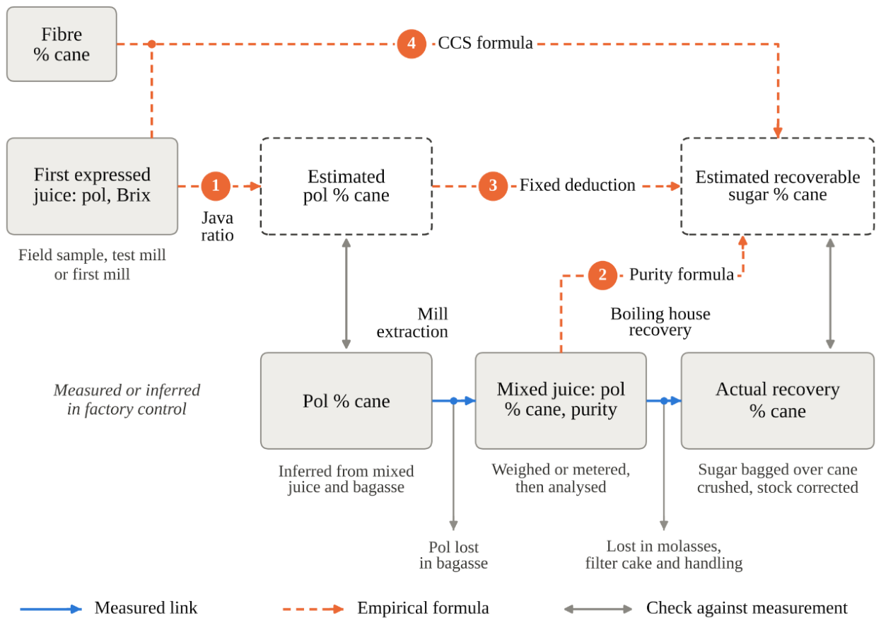
Figure 2.
The Java ratio: theoretical sensitivity and published factory averages. (a) The juice to cane coefficient implied by two fibre conventions, a cane of uniform juice, j = (100 − F)/100, and the Australian CCS convention, j = (100 − (F + 5))/100, set against the guide range of 0.80 ± 0.02 given by Singh (2017). Open circles are the season averages of the twenty South African factories in 1970-71 and open squares those of three other Southern African factories, from Lamusse (1971) as reproduced in Table A1. The dashed line is the least squares fit to the South African factories made for this review (Section 5.4). These observed ratios have the sucrose % cane as numerator and the pol of first expressed juice as denominator, whereas the conventions and the guide range are stated for pol in both terms. The comparison indicates an association with fibre and does not establish that the two bases are equivalent. (b) Pol % cane estimated from the pol of first expressed juice with three assumed coefficients. The shaded band covers coefficients from 0.78 to 0.82. The value 0.72 is an illustrative low coefficient and is not documented in industrial use. The lines in both panels are calculated from the formulas and show how estimates respond to assumptions. They are not measurements of error.
Figure 2.
The Java ratio: theoretical sensitivity and published factory averages. (a) The juice to cane coefficient implied by two fibre conventions, a cane of uniform juice, j = (100 − F)/100, and the Australian CCS convention, j = (100 − (F + 5))/100, set against the guide range of 0.80 ± 0.02 given by Singh (2017). Open circles are the season averages of the twenty South African factories in 1970-71 and open squares those of three other Southern African factories, from Lamusse (1971) as reproduced in Table A1. The dashed line is the least squares fit to the South African factories made for this review (Section 5.4). These observed ratios have the sucrose % cane as numerator and the pol of first expressed juice as denominator, whereas the conventions and the guide range are stated for pol in both terms. The comparison indicates an association with fibre and does not establish that the two bases are equivalent. (b) Pol % cane estimated from the pol of first expressed juice with three assumed coefficients. The shaded band covers coefficients from 0.78 to 0.82. The value 0.72 is an illustrative low coefficient and is not documented in industrial use. The lines in both panels are calculated from the formulas and show how estimates respond to assumptions. They are not measurements of error.
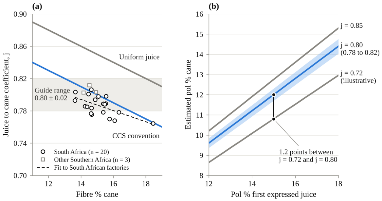
Figure 3.
Illustrative sucrose balance for an Indian plantation white sugar factory, per 100 units of sucrose in cane. Losses in the boiling house are restated on cane. Calculated from the stage figures of Singh (2017).
Figure 3.
Illustrative sucrose balance for an Indian plantation white sugar factory, per 100 units of sucrose in cane. Losses in the boiling house are restated on cane. Calculated from the stage figures of Singh (2017).
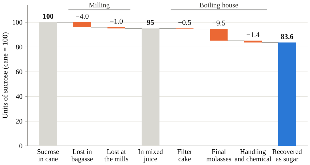
Figure 4.
Recovery estimated from cane pol by two rules, expressed as pol in sugar % cane: a proportional sucrose balance that recovers 83.6% of the pol in cane (Figure 3), and a fixed deduction of 2.5 points, the allowance used by Mehdi et al. (2023). The two agree only near 15.2% pol. Expressed as sugar of 99.8 pol, the balance line would lie less than 0.03 points higher (Section 6.4). Both lines are illustrations calculated from stated assumptions, and neither is fitted to factory data.
Figure 4.
Recovery estimated from cane pol by two rules, expressed as pol in sugar % cane: a proportional sucrose balance that recovers 83.6% of the pol in cane (Figure 3), and a fixed deduction of 2.5 points, the allowance used by Mehdi et al. (2023). The two agree only near 15.2% pol. Expressed as sugar of 99.8 pol, the balance line would lie less than 0.03 points higher (Section 6.4). Both lines are illustrations calculated from stated assumptions, and neither is fitted to factory data.
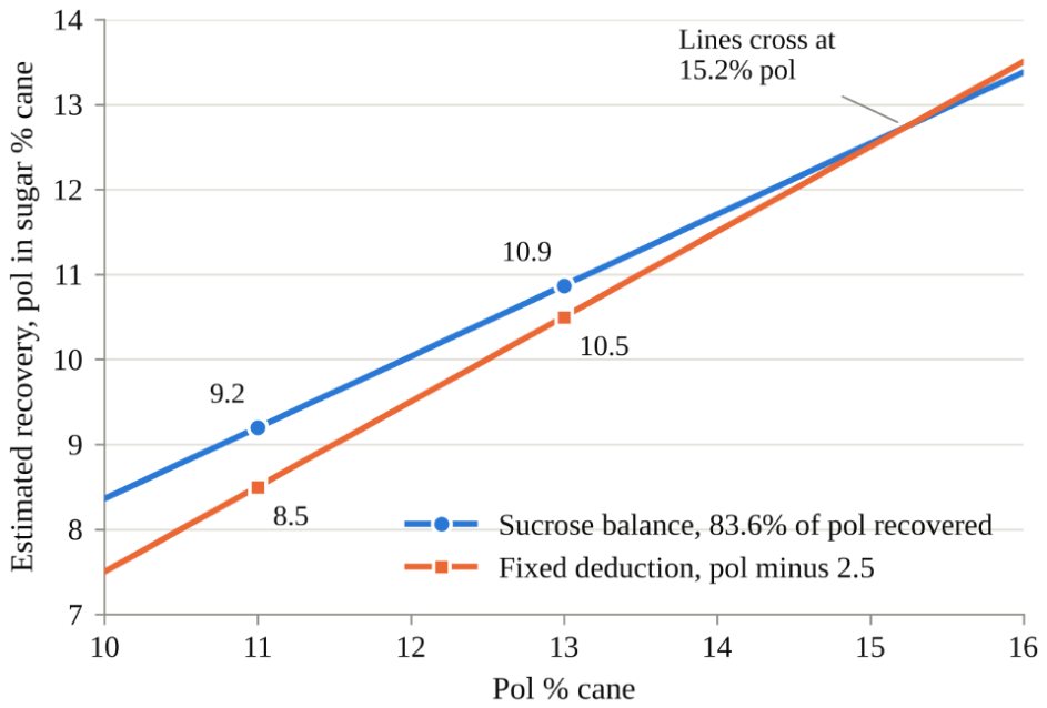
Table 1.
Guide values for cane quality and factory performance in an Indian plantation white sugar factory (Singh 2017). These are a practitioner’s reference points and not industry averages.
Table 1.
Guide values for cane quality and factory performance in an Indian plantation white sugar factory (Singh 2017). These are a practitioner’s reference points and not industry averages.
| Quantity | Guide value |
| Pol % cane | 13.0 ± 0.5 |
| Fibre % cane | 13.5 ± 0.5 |
| Java ratio, % | 80 ± 2 |
| Dry milling factor | 70 ± 2 |
| Sucrose reaching mixed juice, % of sucrose in cane | about 95 |
| Sucrose recovered as sugar, % of sucrose in mixed juice | 88 to 90 |
| Boiling house losses, % of sucrose in mixed juice | 10 to 12 at most |
Table 2.
Fraction of the pol in juice expected as sugar under two purity formulas. The SJM column is the factor in the official Indian formula before multiplication by K. The Winter factor is algebraically identical to the SJM expression with S = 100 and an equivalent parameter of 28.57 in the place of M. The parameter is not an observed molasses purity, and Prinsen Geerligs (1917) applied the factor to raw sugar on a basis of 96 polarisation, so the two columns are not on the same sugar basis.
Table 2.
Fraction of the pol in juice expected as sugar under two purity formulas. The SJM column is the factor in the official Indian formula before multiplication by K. The Winter factor is algebraically identical to the SJM expression with S = 100 and an equivalent parameter of 28.57 in the place of M. The parameter is not an observed molasses purity, and Prinsen Geerligs (1917) applied the factor to raw sugar on a basis of 96 polarisation, so the two columns are not on the same sugar basis.
| Juice purity | SJM factor (S = 100, M = 35.6) | Winter factor (1.4 − 40/purity) |
| 76 | 0.825 | 0.874 |
| 78 | 0.844 | 0.887 |
| 80 | 0.862 | 0.900 |
| 82 | 0.879 | 0.912 |
| 84 | 0.895 | 0.924 |
| 86 | 0.910 | 0.935 |
Table 3.
CCS calculated for a first expressed juice of 16% pol and 19% Brix at three levels of fibre.
Table 3.
CCS calculated for a first expressed juice of 16% pol and 19% Brix at three levels of fibre.
| Fibre % cane | Pol % cane | Brix % cane | CCS |
| 12 | 13.28 | 16.15 | 11.84 |
| 14 | 12.96 | 15.77 | 11.56 |
| 16 | 12.64 | 15.39 | 11.27 |
Table 4.
The empirical methods compared: what each measures and estimates, the assumptions on which it rests, the bias known or expected, and the conditions that call for recalibration. The entries on bias are drawn from the sources cited and from the algebra of the formulas. Except where a measurement is cited, they are not measured errors.
Table 4.
The empirical methods compared: what each measures and estimates, the assumptions on which it rests, the bias known or expected, and the conditions that call for recalibration. The entries on bias are drawn from the sources cited and from the algebra of the formulas. Except where a measurement is cited, they are not measured errors.
| Method | Measured inputs | Quantity estimated | Assumptions | Known or expected bias | Recalibrate when |
| Java ratio with a fixed coefficient | Pol of first expressed juice | Pol % cane | The cane resembles the average on which the coefficient was set, in fibre, trash, maturity and preparation | Makes no allowance for fibre (Kelly 1974). A common ratio favours dirty cane and cane of high fibre over clean cane (Antonowitz 1957) | Variety mix, crop class, trash or season changes |
| Java ratio updated by factory and period | Pol of first expressed juice, with pol % cane from the factory balance of the preceding period | Pol % cane of the current supply | Supply and milling in the current period resemble those of the last | A period average applied to single consignments. It lags behind abrupt changes in the supply | Every period, as Prinsen Geerligs (1917) prescribed |
| Fibre based coefficient (uniform juice or CCS convention) | Pol of first expressed juice and fibre % cane | Pol % cane | A fixed relation between first expressed juice and the whole juice of the cane, with a constant allowance for water held by fibre | No fibre factor is exact (Prinsen Geerligs 1917). In press tests the relation differed between varieties (Brokensha et al. 1976). The error of the fibre figure passes into the estimate | Preparation, mill setting or varieties differ from those behind the allowance |
| Inferential pol % cane | Weights and analyses of mixed juice, imbibition water and bagasse | Pol % cane and fibre % cane of all cane crushed in a period | Each stream is weighed or metered and properly sampled | Reliable only as an average over a period. It carries the errors of bagasse sampling and juice weighing | Not a calibration. Instruments and sampling need routine checks |
| Winter formula | Pol and purity of raw juice | Available sugar of 96 polarisation | Final molasses is exhausted to a constant purity. The factor has the SJM form with an equivalent parameter of 28.57, which is not an observed molasses purity | Approximate. It shifts with the purity to which molasses is exhausted (Prinsen Geerligs 1917) | Molasses exhaustion or the grade of sugar differs from the convention |
| SJM formula in the official Indian form | Pol and purity of mixed juice | Estimated recovery % cane where B heavy molasses or the whole of the juice or syrup is diverted (DFPD 2023) | Sugar purity of 100 and molasses purity of 35.6, with no other loss after mixed juice | Overstates recovery where molasses purity is higher than assumed or other boiling house losses are material | Used outside the cases for which it is given. Under partial diversion the guidelines call for the actual purity of final molasses |
| CCS formula | Pol and Brix of first expressed juice and fibre % cane | Sugar recoverable by a mill of standard efficiency, % cane | The fibre allowances of the formula. Each unit of soluble impurity carries half a unit of sucrose to molasses | Not the recovery of a given factory. It differs with where in a block the sample is cut (Bramley et al. 2012) | Factory efficiency or cane composition departs from the standard behind the formula |
| Recoverable sugar formula with seasonal factors (ERC) | Pol, Brix and moisture of cane by direct analysis | Estimated recoverable crystal % cane | Losses per unit of non pol and of fibre equal those of the factories in the seasons from which the factors were derived | Provisional factors are averages of the two preceding seasons, so estimates differ from those made with the actual factors of the season until payments are adjusted (Mutatu 2023) | Every season, after the products have been reconciled |
| Fixed deduction | Pol % cane, measured or estimated | Recovery % cane | The same number of points is lost whatever the quality of the cane | Implies an overall recovery that rises with cane pol. The loss varies from mill to mill (Mehdi et al. 2023) | Applied outside the experiment or factory for which the allowance was chosen |
| Direct cane analysis (reference) | A weighed sample of prepared cane, analysed directly by a reference method | Pol, Brix and fibre % cane of the sample | The sample represents the consignment | Sampling error. A small sample represents a load or a field poorly. Duplicate standard deviations of 0.3 units for pol and 1.5 for fibre have been reported (Schäffler et al. 2003) | No factor to adjust. Common quality control between mills is needed |
Table 5.
Model classes for the two evaluations of conventional factors. Within each evaluation every model predicts the same target on the same samples or periods, at the same time and from the same information.
Table 5.
Model classes for the two evaluations of conventional factors. Within each evaluation every model predicts the same target on the same samples or periods, at the same time and from the same information.
| Model class | Evaluation 1: pol % cane of a sample or consignment (reference: direct cane analysis) | Evaluation 2: in process forecast of the recovery of a factory over a crushing period (reference: actual recovery) | What the step tests |
| Common time of estimate | When the juice of the sample, and its fibre where a model uses it, have been analysed. The direct analysis is withheld until the estimates are fixed | After the juice and bagasse analyses of the period are available, and before its sugar is bagged and its stock reconciled. Prediction before harvest is a separate task | That every class works from the same information |
| A. Fixed factor | One Java coefficient applied to the pol of first expressed juice | Estimated pol % cane less a fixed deduction, or multiplied by a fixed overall recovery | The baseline in its simplest form |
| B. Conventional correction | Fibre adjusted coefficient of the CCS type, from juice pol and fibre | Purity formula (SJM or Winter) applied to the pol and purity of mixed juice, with CCS as a benchmark estimate | Whether routine fibre and purity data are enough |
| C. Factory calibration | Regression on juice analysis, fibre, variety, crop class and date, fitted at one factory | Sucrose balance with extraction and boiling house terms estimated from earlier periods at the same factory | The value of local calibration, as Prinsen Geerligs prescribed |
| D. Hierarchical model across factories | As C, pooled over factories with an effect for each factory | As C, pooled over factories with an effect for each factory | Whether information transfers between factories. A factory held out of the calibration is predicted from the pooled relation, or with an effect estimated on a separate calibration set of its earlier periods |
Table 6.
Streams of the sucrose balance of a factory over a crushing period. Every quantity is entered in one row only. The last row is obtained by difference, so the rows sum to the input by construction. It is reported separately, as a percentage of the input, and judged against the uncertainty of the measured rows.
Table 6.
Streams of the sucrose balance of a factory over a crushing period. Every quantity is entered in one row only. The last row is obtained by difference, so the rows sum to the input by construction. It is reported separately, as a percentage of the input, and judged against the uncertainty of the measured rows.
| Stream | How it is obtained | Counted as |
| Sucrose in cane crushed | Pol in mixed juice plus pol in bagasse by the inferential method, or direct cane analysis | Input |
| Sugar bagged, by grade | Weighed, with the pol of each grade | Product |
| Change in stock in process | Syrup, massecuite and molasses in process at the end of the period less those at the start, measured and analysed | Stock change, positive or negative |
| Juice or syrup sent to the distillery | Metered and analysed | Ethanol feedstock |
| B heavy molasses sent to the distillery | Weighed and analysed | Ethanol feedstock, and not a molasses loss |
| Final molasses | Weighed and analysed | Loss |
| Bagasse | Quantity by difference, pol analysed | Loss |
| Filter cake | Weighed and analysed | Loss |
| Undetermined (residual) | Input less all the rows above | Residual by difference, reported with its sign as a percentage of the input. It holds unmeasured losses and the net error of every measurement |
Disclaimer/Publisher’s Note: The statements, opinions and data contained in all publications are solely those of the individual author(s) and contributor(s) and not of MDPI and/or the editor(s). MDPI and/or the editor(s) disclaim responsibility for any injury to people or property resulting from any ideas, methods, instructions or products referred to in the content. |
© 2026 by the authors. Licensee MDPI, Basel, Switzerland. This article is an open access article distributed under the terms and conditions of the Creative Commons Attribution (CC BY) license (http://creativecommons.org/licenses/by/4.0/).
Copyright: This open access article is published under a Creative Commons CC BY 4.0 license, which permit the free download, distribution, and reuse, provided that the author and preprint are cited in any reuse.