

Submitted:
14 November 2026
Posted:
18 November 2026
You are already at the latest version
Abstract
Classical preparation records enable conditional control of qubit states but can also make their labels distinguishable. An ideal conditional polarization advantage \( d \) imposes a sharp Helstrom-bias bound \( Q\ge d \); importantly, every source saturating this bound has commuting conditional states. We therefore fix the state-pair commutator norm \( c=\|[\rho_1,\rho_2]\|_1 \) and determine the strictly stronger sharp bound \( Q_{\min}(d,c) \) by optimizing jointly over the prior and both binary-qubit states. Crucially, the same sharp discrimination floor can be attained by distinct global minimizers with different label-blind mean-state purities, measurement decision gains, and Holevo information; at one certified coexistence point, their Holevo quantities differ by about \( 0.0647 \) bit. An analytic canonical reduction and exact computer-assisted comparisons establish a global phase diagram of canonical minimizing representatives, with mixed--pure reentrance and nonlocal exchanges between competing source structures. Thus two constrained source invariants determine an exact minimum-error discrimination floor without uniquely fixing the physical and information resources of its saturating ensembles.
Keywords:
quantum state discrimination
; Helstrom bound
; binary-qubit ensembles
; noncommutativity
; global optimization
1. Introduction
A classical measurement record can change what is achievable with a quantum system. In particular, a controller possessing a preparation label may apply a label-conditioned unitary, whereas a controller without that label is restricted to a common operation. A receiver of the same system, also lacking the individual label, may instead try to infer it by discriminating the conditional states. This raises a question linking control and quantum information: what does an advantage from knowing the record necessarily imply about the label’s distinguishability? Outcome-conditioned quantum control has been demonstrated in superconducting-qubit experiments [13,14]; these provide physical motivation, not an experimental realization of the particular constraints imposed below.
For a binary-qubit ensemble , let be the average length of the conditional Bloch vectors and that of the average state. The difference is the polarization advantage accessible by aligning the states with label-dependent rather than common unitaries. For a fixed qubit Hamiltonian, is also an ideal state-side ergotropy advantage under unrestricted unitary control [20,21,22]; it does not account for information-processing and feedback costs [23]. Two distinct information quantities are the Holevo correlation and the Helstrom bias , which gives the minimum-error success probability [1,2,25]. A nonzero does not, by itself, imply an improved minimum-error decision over guessing the more likely label.
The advantage d alone yields two sharp bounds, and , with in natural entropy units. For , equality requires the two weighted Bloch vectors to have equal lengths and cancel exactly ( in the notation below). Every such saturating state pair is therefore commuting. A symmetric antiparallel ensemble also saturates the Holevo bound. The d-only limits are thus genuinely sharp, but their saturating structures cannot describe how prior asymmetry, mixedness, and noncommuting state geometry compete once the commuting sector is excluded.
This motivates imposing an additional, nonredundant state-pair constraint: the commutator norm . For qubits, , so this rotation-invariant constraint vanishes precisely for commuting states and couples the individual purities to their relative orientation. Unlike overlap or distance measures of the states, it isolates noncommutativity without directly specifying the prior-dependent decision bias. Commutator-based ensemble quantumness has been studied using trace norms and other unitarily invariant norms [15,18], while an alternative measure uses commutators of square-root states [17]. For a binary qubit ensemble, the weighted squared-commutator measure of Song and Li reduces to [19]. We instead fix the unweighted state-pair norm c, so the preparation prior remains an independent optimization variable rather than entering the prescribed measure. State-pair noncommutativity also has operational consequences in other tasks, such as the no-broadcasting theorem [16], but c itself is not a broadcasting error or a universal quantumness measure. Its specific role here is sharper: fixing excludes every saturator of . The resulting strict improvement in the bound is not determined by the equality argument alone; its optimal value and saturating sources require a new constrained optimization. The same two invariants occur together in measurement-conditioned preparation: at fixed input polarization, varying the strength of a symmetric Lüders instrument changes both d and c (Sec. Section 2.3), providing a concrete preparation benchmark.
The relevant distinction from previous state-discrimination research is the outer optimization. Helstrom and geometric methods find optimal measurements or characterize equally distinguishable ensembles for specified discrimination tasks [1,3,4,5,6,9]. Recent structural discrimination bounds also concern measurements and distinguishability under different specified state data [7]. Inverse constructions for pure-state discrimination [10], prior-dependent contextuality in discrimination [8], and minimax optimization of measurement strategies or prior probabilities [11,12] address related but different variables. Here we jointly vary both source states and their prior probabilities while fixing d and c, and determine
The constraints specify a source class rather than a particular fully calibrated preparation device. The precise operational order of the source and measurement optimizations is given in Sec. Section 2.2.
The scope is specific: the receiver knows the realized ensemble but not its individual preparation label. The result therefore bounds ensemble-informed optimal discrimination across the source class, not the performance of a single unknown-source measurement or an adversary’s maximum success rate. The control advantage is an ideal state-side quantity, not a net work balance including implementation and memory costs; c characterizes the conditional states rather than the disturbance of a particular instrument. Critical features below concern the optimizing source family, not equilibrium thermodynamic transitions.
Our solution establishes the exact discrimination floor and shows that its globally minimizing sources need not be physically or informationally equivalent. At a certified B/A–C coexistence, distinct minimizers share but have different majority priors, mean-state polarizations and purities, measurement decision gains, and Holevo information (a difference of about bit at the cited point). Establishing that both sources are globally optimal requires an exact canonical reduction and computer-assisted global comparison. These yield a complete phase diagram of four classes of canonical minimizing representatives, I, B, A, and C. The selected source switches between prior-dominated and measurement-active decisions and between mixed and pure preparations; at the sequence is I–B–A–C–B–A–C as increases. The nonlocal exchanges and certified critical values , , and govern these changes; the narrow contact and annihilation laws are distinct from the broad exchange curves.
These results require a global comparison: at fixed nonzero c, prior, purity, and Bloch geometry generate competing stationary and boundary minima, and local stationarity cannot determine which branch is globally least distinguishable. We first establish canonical representative completeness analytically and then certify the ordering of all physical candidates using exact algebraic computer-assisted comparisons. The main text proceeds from the sharp baseline through the certified phase diagram to the physical and information-theoretic consequences; full root-count and connectivity certificates, mean-polarization-resolved analysis, critical scaling laws, and noise extensions appear in the appendices.
2. Operational Definition and Geometric Reduction
Let be a binary qubit ensemble with , . Set , and
The fixed constraints and discrimination bias are
Our optimization also varies the prior probabilities:
In the physical interior we have the exact identities
with the necessary and sufficient physical conditions
Proof. The Helstrom operator equals , whose trace norm is . The first identity follows by expanding the Euclidean norms. The second identity follows from and . Conversely, physical triples satisfying Eq. (6) reconstruct and ; the triangle inequalities construct their relative angle, while the third inequality guarantees that the Bloch radii do not exceed unity. □
The admissible noncommutativity is where, writing , , and ,
Throughout the phase analysis, c denotes the commutator norm, while is the nonnegative algebraic chart coordinate. We retain the notation when the second argument is the norm itself, and write when using C. For squared-bias singularity calculations we use
These two constraints are not freely independent: their joint feasible region is precisely bounded by Eq. (7). The exceptional points with must be handled directly from the original ensemble definition, not from formulas divided by d.
2.1. Commuting Saturation and the Additional Constraint
The reason for imposing c can be made exact, rather than inferred from a single saturating example. Using Eq. (5),
For , therefore holds if and only if
Indeed requires and follows; conversely these conditions together with the prior restriction give . The antiparallel Bloch vectors commute, hence . Bloch-radius feasibility additionally restricts the prior to ; the complete physical equality range is thus . At fixed d and nonzero c, no equality case survives: by compactness of the constrained physical source family,
This establishes strictness but not the value of the new sharp floor.
There is a parallel, though operationally different, entropy bound. Define with natural logarithms. For the binary ensemble , and convexity and monotonicity of g yield
The explicit commuting source , saturates both bounds. Equation (10) characterizes all discrimination-bound saturators; it does not imply that every one of them also saturates the entropy bound.
Coarse-grained source specification.
The two constraints can be expressed using rotationally invariant state-characterization data. For example, set and . Then
These identities describe what an auditor could calculate from a calibrated source. A two-scalar class report releases only ; all microscopic implementations realizing those values are then included in the family. Complete calibration data would determine Q for a particular source, but would not replace the sharp bound for the whole reported class.
2.2. A Sharp Worst-Source Guarantee
Let denote the compact family of physical binary-qubit ensembles satisfying the two equalities in Eq. (4). Because the optimal receiver may adapt to the realized ensemble, the operational order is
Consequently, every admissible ensemble has minimum achievable error
and the inequality is attained by at least one physical source. For fixed d without a constraint on c, the sharp baseline is . The equality analysis in Sec. Section 2.1 shows why fixing any feasible strictly improves the family-wide floor. Equation (14) fixes the ensemble-informed operational order underlying this class-wide guarantee.
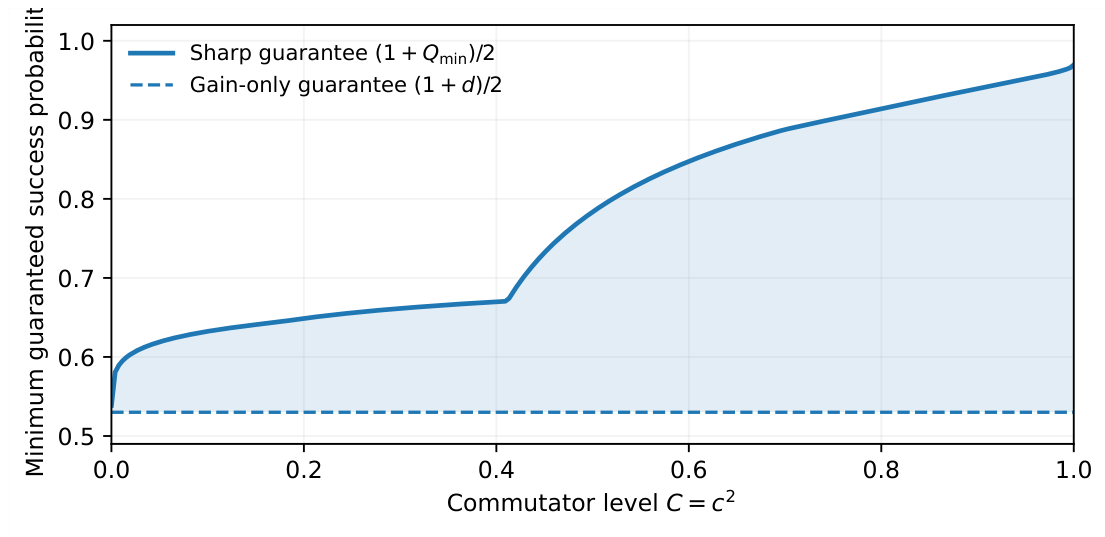
For example, the global equality at has . The control-only baseline is only , whereas the sharp joint-constraint floor is . Importantly, a worst-case B representative already has this success rate by guessing its majority prior; hence the improvement is a statement about total decodability, not necessarily about information gained from a nontrivial measurement. The global phase diagram identifies where the least-favorable source instead requires an active measurement.
Figure 1.
Improvement of the sharp source-family discrimination success floor at . The solid curve is , the dashed line is the sharp d-only floor , and the shading is their difference. The initial rise is linear in [Eq. (25)]. Curves are numerically rendered from the certified candidate equations. Plotting-code development received AI assistance.
Figure 1.
Improvement of the sharp source-family discrimination success floor at . The solid curve is , the dashed line is the sharp d-only floor , and the shading is their difference. The initial rise is linear in [Eq. (25)]. Curves are numerically rendered from the certified candidate equations. Plotting-code development received AI assistance.
2.3. A Physical Benchmark: Symmetric L Üders Conditioning
A simple measurement model illustrates that the constraints need not be assigned to abstract Bloch vectors. Apply the two-outcome Lüders instrument with effects to . Its outcomes have equal probabilities, and the conditional Bloch vectors are , where . Direct evaluation gives
and consequently . For any equal-prior binary-qubit ensemble, and , implying . The Lüders model saturates both geometric inequalities, yielding the sharp equal-prior bound throughout that subfamily’s physical domain. In our main problem the prior is also optimized; hence and the equality need not persist. For example, , , and (corresponding to ) give , , and . At the same constraints, optimization over both states and the prior yields , a reduction of approximately in optimal success probability (about percentage points). This example illustrates a realizable source family, without claiming that it implements all four global phases.
3. Completeness of Extremal Representatives
Theorem 1
(Canonical fixed-prior reduction). Fix , and an admissible . Put , and, after labeling ,
There exists a minimum-bias representative at fixed with
where is unique and
Consequently a minimizing representative has either equal weighted Bloch lengths (the balanced branch) or a pure minority-prior state (). The theorem claims existence of a canonical representative, not uniqueness of every optimum in a prior-dominated flat region.
Proof. For fixed s the exact commutator constraint is maximized by the physical ℓ closest to t; the envelope then decreases strictly in s. The largest admissible s minimizes the active squared bias because and . See Appendix A for the physical seam and attainability argument. □
Choose the label order so , and put . For fixed t, the commutator constraint gives
Hence the smallest physically admissible B is sufficient. Its two possible branches are (balanced weighted Bloch lengths) and saturation of one of the purity bounds, leading to one pure state; the two branches meet smoothly.
3.1. A Usable Sharp Bound
The canonical reduction gives a practical formula at every physically admissible interior pair . Put , , and let be the unique root of from Eq. (19). With
the sharp bound is the following one-variable minimization:
For practical evaluation, solve the strictly monotone equation for each admissible t, evaluate Eq. (22), and minimize over all admissible prior intervals rather than a single local branch. The inner root is monotone and unique; Eq. (22) requires neither a four-parameter state search nor prior knowledge of which I/B/A/C family minimizes. In two important regions it simplifies further:
The I formula uses the physical root in the globally I-dominated region; the C formula applies only where the best fully pure candidate is physical and globally minimal (in particular, and ). At and it gives . The B and A regions are evaluated by Eq. (22) or the boundary stationarity equations; a single globally valid closed elementary expression is not claimed.
A perturbative consequence makes the role of incompatibility explicit. For each fixed the global I family exists for all sufficiently small , and expansion of Eq. (23) yields
In terms of the chart coordinate , this is a rise, continuous at but with an infinite right derivative with respect to C. A natural scaled perturbation parameter is , since ; it is not the sole scaling variable at finite d and the expansion is not uniform as . This is a sharp floor for total minimum-error success, including the prior, not necessarily a minimum gain due to a nontrivial measurement.
Theorem 2
(Representative completeness). In the interior , the global minimum in Eq. (4) has a representative of one of the types I, B, A, C: the prior-dominated balanced branch (I); the prior/measurement threshold on the one-pure-state boundary (B); an active stationary point on that boundary (A); or the fully pure boundary (C). The result guarantees the existence and completeness of these canonical minimizing representatives; it does not classify every noncanonical minimizer in flat objective regions.
Proof. The canonical family has only a balanced and a minority-pure piece. Along the balanced piece an interior minimum occurs only at the prior/active threshold; on the one-pure piece it occurs at an active stationary point or a threshold. The seam is not an extra minimum, and feasible interval endpoints are fully pure. Appendix A treats the physical endpoints, seam derivatives, and compactness in detail. □
Here and in Table 1, and . For the displayed canonical representatives, the open I and B phases admit a prior-only optimal decision, whereas the A and C representatives require an active state measurement. The representative type is thus physically informative even when two types give the same .
On the one-pure-state boundary define , so
Define , and . Active A stationary points satisfy .
Theorem 3
(Global upper bounds for active candidate counts). Let count the physical stationary A candidates satisfying , , and . Separately, let count the physical one-pure B-threshold candidates satisfying and , at the prescribed . Then, on their respective physical domains,
The upper bound for is sharp at , . The B boundary isnotpart of the open active set .
Proof. The single-peaked B boundary gives ; the active A stationary set is split into two physical subdomains controlled by exact Bernstein/Sturm signs. A disjoint rational witness establishes sharpness. The full certificates and domain predicates are recorded in Appendix H. □
4. Global Comparison of Candidate Branches
The representatives in Table 1 are the starting point for the global comparison. Each class can contain stationary or boundary candidates, whose ordering requires more than local optimality. For example, on the fixed- slice the global winner runs through I–B–A–C–B–A–C as grows (Figure 3). A single local expansion or a comparison of one candidate pair cannot certify this sequence or rule out an unseen competitor.
Analytic reduction and connectivity establish candidate completeness; exact Bernstein/Sturm, root-isolation, and interval certificates establish their global ordering on the specified physical domains. Table 2 records the division of proof obligations. The archived PRA_manuscript_code_map.md identifies the corresponding exact predicates, physical parameter domains, executable source paths, and their use in the proof. Independent original-Bloch numerics serve only as crosschecks.
Theorem 4
(Computer-assisted global classification of optimal representatives). Let , , and . The algebraic critical values are isolated by the exact polynomials and physical-root certificates in Appendices Appendix H and Appendix L (certified); numerically,
In the low-noncommutativity region , the globally minimal representatives, in increasing order of C, are
In the nonempty high region (),
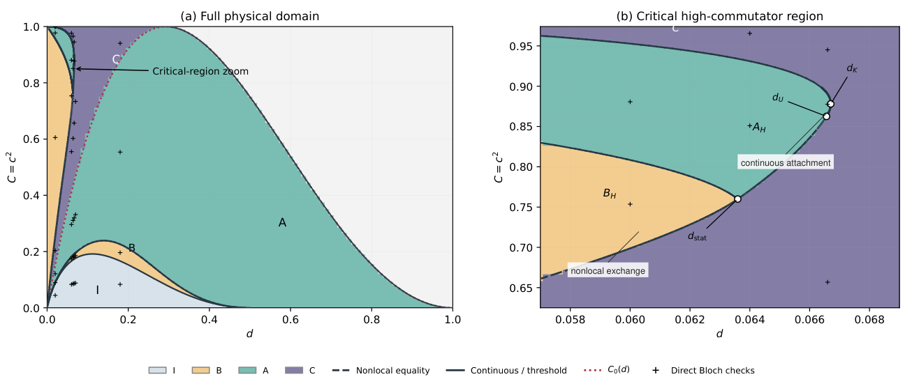
The first high-C transition is a nonlocal –C equality when and a nonlocal –C equality for ; at it becomes continuous. Both transitions in the regime are continuous pure-state attachments. At the open domain collapses. The nonlocal B–C exchange spans , while the nonlocal A–C exchange occurs for ; these phenomena are not confined to the narrow interval , whose width is approximately . The square-root annihilation law at and its local normal form do probe that narrow interval. Transition equalities and the closed physical boundary are classified in Appendix K.
Outline of proof. Theorems 1 and 2 exhaust the physical minimizing representatives. The exact candidate-count certificates and the analytic order-propagation lemma then reduce the global problem to certified candidate attachments, folds, and equal-value crossings. Appendix J.1 establishes the low-C ordering; Appendices Appendix J.2 and Appendix J.3 control the high-C B branch and its nonlocal exchange; and Appendix J.4 treats A–C reentry and annihilation. The closed-domain cases are handled in Appendix K. Each computational exclusion is applied only on its certified physical domain, with the analytic connectivity implications recorded in Appendix J.□
Figure 2.
Global phase diagram of canonical minimizing representatives in the full feasible domain (left) and a critical-region enlargement (right). Colors denote I, B, A, C. Dashed dark curves mark nonlocal exchanges between distinct minimizers, while solid dark curves mark continuous attachments or prior/measurement decision thresholds; the red dotted reference curve is . White circles locate the certified critical values ; plus signs show independent direct Bloch checks. The inset labels identify an exchange and a continuous attachment. Boundaries are numerically rendered from the certified candidate equations. Plotting-code development received AI assistance.
Figure 2.
Global phase diagram of canonical minimizing representatives in the full feasible domain (left) and a critical-region enlargement (right). Colors denote I, B, A, C. Dashed dark curves mark nonlocal exchanges between distinct minimizers, while solid dark curves mark continuous attachments or prior/measurement decision thresholds; the red dotted reference curve is . White circles locate the certified critical values ; plus signs show independent direct Bloch checks. The inset labels identify an exchange and a continuous attachment. Boundaries are numerically rendered from the certified candidate equations. Plotting-code development received AI assistance.
Unreduced-variable crosscheck.
We also optimized in the original physical Bloch variables without constraining the search to the canonical family. At 34 source-interior samples the maximum observed objective discrepancy was and the commutator-constraint residual was . Independently derived physical boundary equations reproduced 22 transition locations to within of numerical phase-label extractions. The direct optimization and comparison data are described in Appendix D; the global logical dependencies are given in Table 2.
5. Operational and Information-Theoretic Consequences
The fixed quantity d quantifies an ideal conditional-control opportunity, whereas the globally minimized Q quantifies the difficulty of identifying an unknown preparation label. They characterize different operational tasks. A controller who knows the label and can apply unrestricted conditional unitaries aligns the weighted Bloch vectors, increasing the mean polarization from B to R. Relative to the best label-blind unitary,
For the corresponding ideal available-energy advantage is . The label-blind observer instead has
The geometric bound implies , with a strict inequality for : .
Theorem 5
(Decision threshold versus acquired information). On nondegenerate global I/B representatives, ; on measurement-active A/C representatives, . Nevertheless a B-type representative can admit a Helstrom-optimal two-outcome measurement with positive mutual information despite . For a one-pure-state representative with majority prior , minority prior , and , the exact Holevo quantity (in bits) and the pure-C quantity are
where is the binary entropy. The Holevo quantity is defined as the entropy difference [25]. Thus the pure-C Holevo quantity at fixed d is constant in C, although the optimal prior and Helstrom success rate generally vary with C.
Proof. The Helstrom eigenvalues are . Hence ; I/B have the threshold , while A/C have on their active interiors. On the B threshold and its null projector yields a valid minimum-error-optimal measurement. Its null-outcome probability is , with posterior , and the other posterior is . Thus
for an interior B representative. The constant-majority rule has the same minimum error but zero measurement mutual information. This distinction is consistent with the wider separation between measurements maximizing accessible information and those minimizing error [27,31]. Recent work on information–error tradeoffs further exhibits changes of the optimal measurement at fixed source states [28]; the exchanges considered here are instead between different globally minimizing sources at fixed . Finally, the one-pure Bloch radii are , and the mean radius is . Their qubit spectra immediately give Eq. (35); taking proves the C formula. □
In fact, when is full rank and is pure, the max-relative-entropy decision threshold [26] has the exact form
Thus the condition is a threshold of the weighted hypothesis-test operator, not the disappearance of all information in the ensemble.
Proposition 1
(Distinct information resources on a global tie). At and the two physically distinct global minimizing representatives, B/A and pure C, have the same but strictly different average-state Bloch radii, average-state purities, decision gains, and Holevo quantities. Writing for the one-pure representative’s purity deficit, the mean-state difference is exactly
The information differences are
Proof. The exact C/D algebraic root isolation puts the physical B point inside , and . Because and , the mean radii are and ; the qubit purity formula yields Eq. (38) with strictly positive difference. Equality of the squared bias implies , hence . Differentiating Eq. (35) at fixed gives
The exact difference of denominator and numerator is , strictly positive throughout the root box. It remains positive for all ; integrating Eq. (40) proves . The displayed decimal values are numerical crosschecks, not the sign proof. □
The two global minimizers can also be exhibited directly as physical qubit preparations. In a common Bloch frame, taking , one realization is
Both reproduce up to rounding; the exact equality and global optimality rely on the algebraically isolated representatives of Theorem 4, not on the displayed decimals.
Table 3 makes the structural exchange visible without conditioning on a chosen measurement: the label-blind average state has a different Bloch radius and purity in the two sources, even though the optimal single-copy label success rate and the constraints agree. The B/A source is prior-dominated, while the pure-C source gains an additional in success probability from measurement. In the same way, the broader certified B–C exchange has and at a common . These values compare canonical global representatives; the full argmin-set distinction is made explicit below.
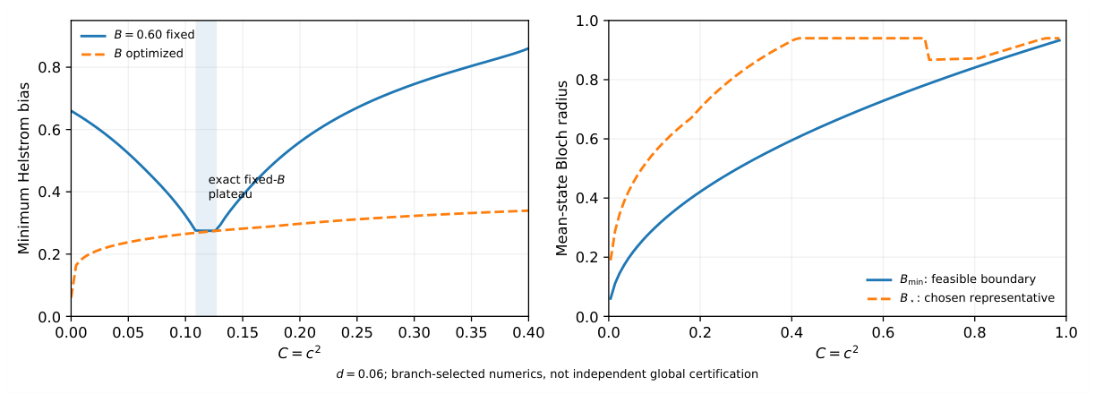
A related but distinct refinement fixes the average-state radius B itself. The resolved floor obeys over physical B. At fixed B, the floor can decrease or remain exactly constant as c changes, despite the strict improvement over in the free-B problem. The exact feasible region, fixed-B proposition, flat interval, and the corresponding figure are given in Appendix B. Fixing B constrains mean-state mixedness and cannot be interpreted as removing prior effects alone.
At a nonlocal tie the optimal information data are naturally set valued. Let denote the full set of physical ensembles satisfying and that attain , and define and . A branch-selected canonical value of or need not be shared by all minimizers, particularly in prior-dominated flat regions; a difference between selected branch values is not an intrinsically single-valued jump of either quantity.
The global reentrance has an operational consequence: for fixed and increasing , the selected minimizer passes through . Its decision advantage correspondingly follows on the respective open phases. In particular, increasing state-pair noncommutativity does not impose monotonicity of the decision advantage of the globally worst ensemble when the prior and both states are free to vary. At the nonlocal C–B equality, contains the two branch values; this is not an asserted single-valued jump.
Further information singularities.
The same global diagram controls how information differences vanish where distinct optimal branches meet: the A–C Holevo difference may have an law, although its decision-gain difference vanishes linearly. At the upper active-phase annihilation the entropy and decision scales differ again. These secondary asymptotics and the low-C spectral boundary law are stated and proved in Appendix O.
6. Discussion and Conclusions
The elementary control–discrimination inequality is sharp, but its equality cases require exactly cancelling weighted Bloch vectors and hence commuting conditional states. This is the specific limitation resolved here: once the additional commutator constraint forbids every saturator, the precise new minimum cannot be inferred from the original inequality or from a local candidate. Our canonical reduction and globally certified I/B/A/C classification give the sharp bound , the physical structures attaining it, and the exchange and attachment curves that select among them. The broad nonlocal exchanges should be distinguished from the much narrower upper critical window.
The phase structure is not merely a catalog of algebraic branches. In the prior-dominated I/B regions a source may attain the minimum bias without any decision improvement from measuring the quantum state; the measurement-active A/C regions are different. The mean-polarization-resolved comparison in Appendix B shows why this competition is not reducible to a prior-only bias: noncommutativity can decrease a fixed-B floor while the free-B sharp floor remains strictly above d. At a nonlocal exchange, the same can be realized by globally minimizing sources with different label-blind mean-state purities, decision gains, and Holevo information. Thus a pair of physical constraints fixes a sharp discrimination floor, but need not fix the information properties of the sources saturating that floor. The local critical laws describe changes in the optimized representative diagram.
Critical geometry and noise paths.
The three distinguished values have different roles in the certified classification (Theorem 4). At a nonlocal B/A–C coexistence yields a derivative kink in the squared minimum bias; at the nonlocal exchange terminates in a continuous pure-state attachment with a one-sided splitting; at the open one-pure active phase disappears, with its width vanishing as . The final narrow region should not be conflated with the broader nonlocal exchange curves. Exact local coefficients are given in Appendix O. Under common depolarization of a fixed source, and ; the actual Helstrom bias and the reoptimized source-family bound generally differ. Their monotonicity and strong-noise scaling are developed in Appendix E, without treating them as primary claims of the present work.
The symmetric Lüders instrument in Sec. Section 2.3 generates d and c jointly and saturates the sharp equal-prior bound; the freely optimized prior can yield a smaller bias at the same constraints. In finite-sample source characterization, confidence regions for would replace exact point specifications, and the corresponding guaranteed floor would be the infimum over that region. Device-specific control of both invariants remains a separate experimental question.
The binary-qubit setting is the minimal regime where noncommuting conditional states, variable preparation priors, and mixedness can compete while the two-eigenvalue Helstrom norm admits an exact Bloch-geometric reduction. The two-state cancellation principle is not intrinsically restricted to qubits: in any finite dimension, writing with traceless Hermitian , the equality implies . For three or more qubit states, in contrast, noncommuting weighted Bloch vectors can already cancel in their mean. The cancellation implication and the distinction between prior-only and measurement-assisted binary decisions can thus survive in higher dimensions, although neither the qubit-specific equality criterion for nor our I/B/A/C diagram has been established there. The present result is an exactly resolved minimal nontrivial regime, not a claim that its complete phase structure is universal.
The classification suggests three concrete extensions. Fixing or constraining the preparation prior would separate prior-only guessing from the additional decision value of quantum measurement and enable sharper comparisons with Holevo and accessible information. General noise channels, finite conditional-control budgets, and repeated measurement–feedback dynamics could connect the static polarization advantage to dynamical performance and actual resource expenditures; those quantities require new assumptions beyond the present model. Coherent quantum side information belongs to a further, distinct feedback-control setting [24]. Related recent approaches explore prior-dependent ensemble responses and different constrained distinguishability questions [29,30]. Extending the present classification to multistate or higher-dimensional sources would require new geometric and spectral methods; the surviving two-state cancellation identity alone does not imply an unchanged phase diagram. These are future questions rather than conclusions of the present classification.
AI-Assisted Research Disclosure: During the preparation of this work, OpenAI ChatGPT (GPT-6) was used to assist with exploring mathematical arguments and derivations, developing and debugging Python verification code, computational checks, literature searches, figure preparation, and manuscript drafting and editing. The research objectives and verification procedures were directed by the author. All mathematical proofs, computational results, and cited references were independently reviewed and verified by the author, who assumes full responsibility for the content.
Data Availability Statement
The source code, exact algebraic certificates, domain records, and reproducibility materials supporting the computer-assisted global classification (Theorem 4) are publicly available in the Zenodo version 0.2.1 archive [32], at https://doi.org/10.5281/zenodo.24013812. The archive includes the 25-suite A–E certificate driver PRA_verify_all_v5.py, the unified release verifier PRA_release_verify.py, the exact high-B inward verifier PRAG3Binwardcertificate.py, supplementary G2–G5 programs, execution instructions, proof-to-code correspondence records, and SHA-256 file-integrity manifests. The complete reproduction command is python PRA_release_verify.py –full, run from the extracted PRA_Zenodo_Release_0.2.1 directory. The analytic arguments connecting the computational certificates to the global classification are provided in Appendices Appendix H–Appendix J. Independent numerical crosschecks are described in the manuscript.
Conflicts of Interest
The author declares no conflicts of interest.
Appendix A. Full Proofs of the Canonical Reduction and Representative Completeness
The proof sketches in the main text have the following detailed algebraic and endpoint justifications. In particular, the seam cannot produce an unlisted canonical minimizer.
Appendix A.0.0.5. Canonical fixed-prior reduction.
Proof. With , the physical deficits satisfy , , , and
At fixed s, the right-hand side is maximized by choosing the physically allowed ℓ closest to t. The constraints on and show that this choice is , giving . For , both positive-factor pieces in Eq. (19) are strictly decreasing on their corresponding ranges and agree at ; . Thus the attainable target fixes a unique , and any other admissible state has . The canonical weighted lengths are nonnegative and obey , so a physical Bloch angle realizes precisely the target C.
Eliminating with the commutator equality yields
Since , maximizing the physically attainable s minimizes J and hence . This proves the claim. □
Appendix A.0.0.6. Representative completeness.
Proof. The fixed-prior canonical reduction (Theorem 1) first eliminates every noncanonical interior configuration and the majority-only-pure boundary as possible sources of a smaller value. It remains to minimize over the compact, physically admissible interval(s) of t after the canonical reconstruction. We classify all possible interior and endpoint minima, including the balanced/one-pure seam.
Balanced interior. On , the canonical state has and , with . At fixed the defining equation is
Writing its positive numerator as gives . Since on the physical interior, implicit differentiation yields
Thus the active term strictly decreases while t strictly increases. Any interior minimum of therefore lies at their equality , namely representative I. A prior-dominated balanced interval cannot provide a new interior minimum.
The seam. At the two canonical pieces meet. Both satisfy and (partials are evaluated at the seam), so from either side; the first derivatives also agree. On the one-pure side, , , whereas on the balanced side . Hence
If , the discrimination bias decreases through the seam; if , it equals the strictly increasing function t there. Neither case admits a local seam minimum. The remaining case is already an I/B threshold representative, not an additional family. The special seam at is addressed below.
One-pure interior. On , is smooth. In an active interior (), a minimum requires at fixed , producing type A. In a strictly prior-dominated interior (), the objective is and increases with t, so no interior minimum occurs. If the two terms meet (), the point is of type B; this includes any optimal kink separating the active and prior-dominated regimes.
Physical endpoints. For , the two weighted Bloch vectors are nonzero and noncollinear. Consequently , so ; the endpoint is never admissible. Any other endpoint of a feasible t-interval with must saturate , since otherwise the canonical construction stays admissible in a neighborhood. Such an endpoint has , hence both states are pure: type C. At , feasibility implies . If , then and for all sufficiently small the canonical branch stays balanced. The strict decrease of for excludes as a minimum. If , then and the endpoint is again pure (type C). For , is inadmissible.
Finally, the ensemble parameter space is compact, the two equalities and define a closed subset, and Q is continuous. A minimum therefore exists. The preceding interior, seam, and endpoint classification exhausts all its possible canonical locations, proving I/B/A/C completeness. This is an analytic proof conditional on the preceding canonical reduction; no stationary-root count or computer certificate is needed for this existence classification. □
Appendix A.0.0.7. Finite active candidate bounds.
Proof. For B, a rational one-parameter representation gives a single-humped noncommutativity curve, as shown by a global Bernstein sign-variation certificate; Rolle’s theorem gives at most two intersections with each level. For A, exact signs split the physical stationary set into a low and a high t regime, with and , respectively. The low regime has a single monotone graph. On the high regime, exact Bernstein/Sturm certificates bound the number of physical connected graph components (or critical points of the single algebraic graph) and show at most two intersections. Independent disjoint rational isolating rectangles establish the sharpness witness. Details of all algebraic domain reductions are in Appendix H and the reproducible source program. □
Appendix B. Fixed-Mean-Polarization Floor and Geometry
The following auxiliary result resolves the mean-state Bloch radius B rather than optimizing it away. It refines the global problem without changing the certified phase classification.
Appendix B.0.0.8. Exact resolved floor.
The average-state Bloch radius B is itself an operationally interpretable invariant: an observer without the preparation label sees mean-state polarization B, or equivalently a mean-state purity . It is useful to distinguish the present free-B problem from the mean-polarization-resolved floor
where is the physically realizable set. This is a refinement by the average state, not a restriction that fixes the preparation prior.
Proposition A1
(Fixed-mean-polarization discrimination floor). Let , , , and . For any physically admissible , the minimum in Eq. (A4) is attained at thesmallest physically admissibleprior bias . In particular, . At fixed , the function need not increase with c; indeed it has an exactly flat interval whenever . For , the allowed mean polarization obeys .
Proof. For choose the sign of K that minimizes its distance from t. Eliminating using Eq. (5) yields
its two entries are nondecreasing on . The exact physical domain, positivity of , and the flat-interval formula are established below. □
Appendix B.0.0.9. Full physical-domain proof.
Let , , , , , , and . Relabel the states so . Because the objective and commutator identity depend only on , and for , every feasible configuration has an equally good representative with . Equations (5)–(6) then give the following necessary and sufficient domain:
For , feasibility implies and . Eliminating k gives the equivalent scalar test
For a physical C this feasible set is compact; the objective
is nondecreasing in , since the derivative of its second entry squared is . Thus the smallest feasible t globally minimizes Q on a fixed- fiber, even when that fiber has disconnected scalar pieces. At , choose in Eq. (A6); then . The lower bound for follows directly from Eq. (5), proving the commuting formula.
At fixed , put
For each t the smallest feasible k is , which maximizes C. Therefore the exact commutator capacity is
The admissible polygon is compact and connected. The continuous image therefore fills the entire interval (the value 0 is attained at ). For fixed , the capacity numerator is for , and for . Both are strictly increasing in and D increases with B. Thus is continuous and strictly increasing from 0 at to the overall physical capacity at . In particular, for every physical there is a unique with , and the feasible mean polarizations are precisely . Because , this also gives a simple, generally nonsharp geometric bound:
The maximum in Eq. (A10) can be evaluated from its endpoints and its interior stationary roots. On the piece they satisfy
Finally, a nonzero commutator need not monotonically raise the fixed-B floor. The universal fixed-B geometric bound is saturated if and . Here requires , while the exact commutator condition gives . Consequently, for , throughout the exact interval
For example, at , , one has , , and the plateau runs from to approximately , with . Outside this interval the physical minimal prior and the geometric term may compete, producing a nonmonotone fixed-B floor without contradicting the global strict inequality .
Appendix B.0.0.10. Physical interpretation and numerical illustration.
This comparison exposes two distinct and competing effects. At fixed , a nonzero commutator can lower the geometric discrimination term in Eq. (A5); on the other hand it restricts the admissible B and prior. For instance, for and the exact fixed-B floor is at , approximately at , and approximately at . By contrast, the free-B floor is strictly larger than d for every admissible . The difference between these floors cannot be identified with a prior-only effect, since constraining B also constrains the mixedness of the average state. Figure A1 illustrates the two optimizations.
On the certified B–C exchange, near , the pure C representative has while the one-pure B representative has , although both attain . Their prior biases are respectively and , so the C representative receives an additional positive decision gain from measurement while the B representative does not. The exchange therefore changes not only source purity but also the mean state and the balance of prior guessing versus measurement. The crossing decimals illustrate a transition whose global existence and ordering follow from Theorem 4.
Figure A1.
Mean-polarization-resolved interpretation on the slice (numerical evaluation of the analytic one-variable reductions). Left: the sharp floor with fixed and the smaller floor with B optimized; the short horizontal segment marks the exactly derived fixed-B plateau. Right: the minimum physically permitted average polarization and a branch-selected minimizing representative . The latter can switch discontinuously at a nonlocal equal-value crossing. The curves illustrate, but do not certify, the global phase classification of Theorem 4. Plotting-code development received AI assistance.
Figure A1.
Mean-polarization-resolved interpretation on the slice (numerical evaluation of the analytic one-variable reductions). Left: the sharp floor with fixed and the smaller floor with B optimized; the short horizontal segment marks the exactly derived fixed-B plateau. Right: the minimum physically permitted average polarization and a branch-selected minimizing representative . The latter can switch discontinuously at a nonlocal equal-value crossing. The curves illustrate, but do not certify, the global phase classification of Theorem 4. Plotting-code development received AI assistance.
Appendix C. Exact Candidate-Comparison Lemmas
These lemmas form the input predicates for the global classification; strict physical-domain and root-selection conditions are part of each statement, and the unabridged rational records are supplied in the reproducibility data.
Appendix C.0.0.11. Candidate comparison setup.
We first certify the candidate comparisons, then use global topology, physical-domain enclosures, and strict derivative orientations to establish which equalities actually exchange the global minimizer.
Lemma A1
(Exclusion of the I branch for high noncommutativity). For , let and . Then ; hence I cannot minimize when .
Proof. The balanced-branch geometry and bound its noncommutativity by . The positivity of on is reduced to a 12th-degree exact rational polynomial whose Bernstein coefficients are all strictly positive. For , the nondegenerate I branch is absent. □
Lemma A2
(Exact B–C candidate comparison). Write , with , and impose the B-threshold condition . There is an integer polynomial of degrees and 193 nonzero terms such that the sign of the difference between B’s noncommutativity and that of a formal equally distinguishable pure candidate is determined by P. On the physical high-C branch, means that the best pure C candidate strictly improves the B candidate.
Proof. Insert and into
The identity shows the sign equivalence after all denominators have been checked positive. The polynomial identity and global root count are independently checked by exact rational arithmetic. □
Lemma A3
(Uniform small-d B–A crossing and stability levels). For , the B–A boundary stationarity polynomial has precisely two zeros in , with
The corresponding B-boundary noncommutativity satisfies
where is the upper pure-stability contact. In the same range, , and for .
Proof. Clearing the physical positive denominators in yields a polynomial with degrees and exactly 126 monomials. Under its z coefficients have a parameter-uniform sign pattern . Descartes’ bound is two, and exact Bernstein evaluations at establish exactly two roots in the stated intervals. Separate two-variable Bernstein coefficients establish the level bounds in those two strips. The pure-stability quartic has the parameter-uniform positive-root sign pattern and exact opposite endpoint signs at ; it therefore has precisely two positive roots in the relevant pure interval. Evaluating at these rational comparison points, and using the fact that has a single maximum, gives and the stated upper-contact margin. The exact polynomial sign checks and their full domains are implemented in the independent 26-check certificate. □
Lemma A4
(Removal of high-C B minima above ). For , , no B candidate is globally minimizing.
Proof. At one has a unique physical common root of with . For exact Bernstein signs show : the outside regions in x have , while and in the central regions. A rational Krawczyk map gives root existence and uniqueness, rather than just a numerical approximation. If , moving into the interior reduces J; if , the pure C candidate reduces Q. For , exact Bernstein signs certify over all physically relevant x. The intervals overlap at , and cover .
The inward-decrease implication requires a separate direction test; by itself does not select the physically active side. Along a regular fixed-C curve on the one-pure boundary, , and the boundary identity gives
For and , the separately distributed exact Bernstein check proves : after , the factorized rational derivative has a bidegree- polynomial factor with all 130 rectangular Bernstein coefficients strictly positive. Its remaining factors have certified signs (see Appendix N and PRA_G3_B_inward_certificate.py). The original certificate separately proves there; its outer-strip tests confine every relevant boundary point to . Thus implies and . Decreasing ℓ at fixed C moves into while lowering J and hence the active Helstrom bias. These signs supply the local physical descent claimed above, not a global-minimality conclusion in isolation. □
Lemma A5
(Pure C wins below the high-C reentry strip). For and , the best fully pure representative is globally optimal, conditional on Theorem 2.
Proof. The mixed/pure comparison at equal candidate squared bias is reduced to
The apparent ℓ denominator cancels exactly, leaving a polynomial of degrees with 78 terms. We first prove that the box used by the 113-node Bernstein comparison includes every candidate that could possibly beat the best pure state, rather than every physically admissible mixed state.
Set and let for the best pure representative with . For , exact rational univariate Bernstein coefficients give . Since and for in this band, the specified implies .
For any non-pure one-pure candidate with , put , so . If , then . Writing and using gives
The second upper bound follows from , which makes the middle expression nonincreasing in ; the lower bound uses . Also . Hence every possible non-pure competitor with lies in the exact rational box , , .
The 113-node exact rational Bernstein tree then gives throughout that box. Since all displayed prefactors are positive for , this requires . But and is strictly increasing there, a contradiction. Thus no non-pure one-pure candidate can tie or beat C; I was already excluded by . The rational enclosure inequalities are independently reproduced by the five-check PRA_G4_physical_cover_checks.py verifier. □
Appendix D. Direct Original-Variable Optimization Checks
The following independent numerical reconstruction starts from the physical Bloch parameters and not the canonical mixing variables.
Appendix D.0.0.12. Independent optimization in the unreduced physical ensemble space.
To check that the plotted regions are not artifacts of the canonical reduction, we separately optimized the physical Bloch parameters without imposing any I/A/B/C representative restriction. At fixed , set , , and . The fixed-d equation directly fixes . Writing and , the original commutator constraint is
For any admissible , the equation for has a unique positive root. Thus one can impose both constraints exactly while optimizing over the entire remaining physical parameter domain, without using canonical mixing variables or a preferred purity face. A differential-evolution search supplemented by separate checks of all physical boundary faces reproduces the candidate objective at 34 independent phase-interior sample points: the maximum observed is and the maximum C-constraint residual is . Seven additional constrained local optimizations in all three original parameters provide a second crosscheck.
For representative d-slices, the physical one-pure face can be evaluated directly without canonical variables. Its conditions and isolate the B–A contacts; comparison with a fully pure competitor isolates nonlocal B–C and A–C ties; and the one-sided pure-face derivative isolates continuous A–C attachments. These direct physical equations reproduce 22 independently computed transition locations at . The largest difference from numerically extracted canonical phase boundaries is , attributable to the finite-resolution numerical phase-label classifier. The exact physical-derivative contact values agree with their independently evaluated stability-quartic roots to about in the sampled cases. For illustration, the six physically derived transition levels at , in increasing order, are
The corresponding representative sequence is . These optimization experiments are numerical crosschecks, not additional global optimality certificates; at equality curves the argmin may be set-valued and a numerical minimizer need not have a unique representative label.
Appendix E. Depolarization and Reoptimization: Secondary Extension
To test the phase structure along a standard physical noise family, consider the same isotropic depolarizing channel acting on both signal states,
The prior is unchanged and each Bloch vector contracts by . Therefore a fixed initial ensemble with is carried to
A fixed physical ensemble and a newly optimized ensemble at the transformed are different experiments. In the former, remains fixed and, writing ,
In the latter the prior and both states may be redesigned at each , so . The dimensionless ratio
is invariant for : the noise trajectory is a parabola in the constrained-ensemble plane.
Proposition A2
(Monotone reoptimized discrimination under depolarization). For and every initially feasible pair ,
Proof. For , apply to any ensemble feasible at the second constraint pair. Equation (A23) proves feasibility at the first pair, and the corresponding Helstrom norm changes from to , which cannot increase. Taking the infimum proves the result. The case is immediate. □
This elementary data-processing consequence should not be confused with a monotonicity theorem for the selected prior, the selected Holevo quantity, or every fixed-ensemble measurement advantage.
Theorem A1
(Strong-noise canonical scaling). Fix and set , . There exists a sufficiently small λ interval on which the global canonical minimizer is of type I. Let be the unique real solution on of
Then
For thecanonicalI representative, whose Holevo information is measured in bits,
These relations do not assert the same limit forallminimum-error-optimal ensembles in a prior-dominated flat set.
Proof. Along Eq. (A23), , whereas the I–B contact has . The global low-C phase theorem thus places the canonical optimum in I for sufficiently small . On I, , and the exact level equation is
Put . Then . At the cubic is negative at , strictly increasing for , and has one zero . Because , the implicit-function theorem expands z analytically in and gives , proving Eq. (A28).
The I branch has , , and . Expanding for these three Bloch lengths produces . The limit follows by division. Equivalently, if , then the strong-noise scaling function obeys the dimensionless equation
□
Proposition A3
(Leading Holevo comparison for a pure initial pair). Suppose the two initial states are pure and . For thefixed noisy ensemble,
If , the sign for sufficiently small is
The equality case requires higher-order comparison.
Proof. The initial mean-state radius is , hence the two state spectra give . To compare the leading coefficients, note that the cubic increases for . At it equals . Therefore has the sign of , equivalently . □
This is a comparison between different ensembles, not a monotonicity of information along a single evolving source. The ideal conditional polarization advantage contracts linearly, whereas the two Holevo quantities in this comparison contract quadratically; neither scaling measures an implementation’s net work cost.
Figure A2.
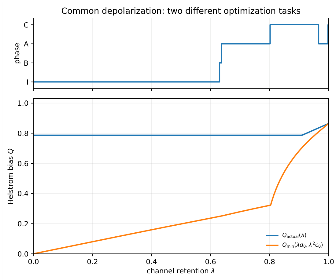
Numerically reoptimized ensemble phases (upper panel) and Helstrom biases (lower panel) along a common-depolarization path starting from a pure representative at , . The actual source retains its initial prior and states, so ; the reoptimized curve minimizes anew at each transformed constraint pair. The phase labels concern reoptimized representatives, not transitions undergone by the same physical state. The plotted phase change positions are numerical illustrations. Plotting-code development received AI assistance.
Figure A2.
Numerically reoptimized ensemble phases (upper panel) and Helstrom biases (lower panel) along a common-depolarization path starting from a pure representative at , . The actual source retains its initial prior and states, so ; the reoptimized curve minimizes anew at each transformed constraint pair. The phase labels concern reoptimized representatives, not transitions undergone by the same physical state. The plotted phase change positions are numerical illustrations. Plotting-code development received AI assistance.
Appendix F. Numerical Illustrations and Canonical Reconstruction
Figure 3 and Figure A2 are generated by minimizing the single-variable canonical objective at each physically permitted prior bias. For fixed one may scan over intervals where , invert the monotone map , and minimize
The formula directly reconstructs each selected prior, purity, and geometric objective without accessing an unconstrained Bloch-angle search. The figures use floating-point root bracketing; certification of physical root counts and branch exchange is supplied separately in the exact source programs and in the proof of Theorem 4. For the strong-noise equation, the statement is uniform on a sufficiently small neighborhood for each fixed nondegenerate initial ; no uniformity is claimed as or approaches zero.
Appendix G. Scope of Analytic and Computer-Assisted Statements
Theorem 1 and the representative-completeness Theorem 2 have analytic geometric proofs that do not rely on root-count certificates. The finite stationary-root bounds and the signs of the algebraic comparison polynomials are computer-assisted: the cited rational Bernstein/Sturm tests certify specific inequalities on explicitly defined domains. Theorem 4 additionally uses analytic branch connectivity, physical boundary classification, and continuity of competitor values. The closed-domain endpoint identities and their equality sets are checked independently in PRA_G5_boundary_certificate.py; the strict interior transition equalities continue to depend on the global certificates. The critical singularity and information theorems depend on that global branch selection and on exact isolated critical-root certificates. The unconstrained Bloch numerics in Sec. Section 4 are independent checks, not a proof of global optimality.
Appendix G.0.0.13. AI-assisted development and validation procedure.
OpenAI ChatGPT (GPT-6) assisted mathematical exploration and the preparation, debugging, and documentation of selected symbolic and numerical Python programs used in this work. The author directed the mathematical questions and the choice of exact predicates and physical parameter domains, then reviewed the relevant derivations, executable assertions, source hashes, and verification outputs. In particular, AI-generated suggestions or program outputs were not treated as proof independently of the exact rational/algebraic checks and the analytic implications given in Appendix J. The use of AI for manuscript and figure preparation is also disclosed below.
Appendix H. Machine-Checkable Algebraic Certificates
The source program PRA_verify_all_v5.py contains plain readable source text for each underlying certificate and extracts uncompressed .py files automatically. Its default run executes the original Bernstein/Sturm/interval certificates for the geometric reduction, stationary point counts, branch comparisons, A–C connection, and reentry. Verification requires Python 3.11 or later, SymPy, NumPy, and mpmath; python -m pip install sympy numpy mpmath provides the declared packages. The retained full run used Python 3.13.5 and took about 241 s in sum of 25 subprocess timings (a machine-specific figure). The 25 suites comprise one A suite, four B suites, 18 C suites, one D suite, and one E suite; the E suite checks 45 symbolic/rational predicates and three separately labeled numerical crosschecks. The 65 SHA-256 values count distinct embedded source/input texts, not 65 independent theorems or test suites. A zero exit status and matching exact assertion signatures validate the stated sublemmas on their specified regions. The precise rational domains and assertion outputs are stored with the source scripts. The single-command suite executes 25 executable computational suites (including the 27-predicate global-closure bridge) and checks 65 source/input SHA-256 hashes. The global comparison uses these predicates as detailed in Appendix J.
Appendix I. Exact Comparison Polynomials and Parameter Covers
For reproducibility the one-pure-state rational level is
with , , and . The formal equal-bias pure comparator is . The normalized A–C tie and active stationarity polynomials are
Their degrees in are respectively , , and . A necessary condition for a nontrivial active nonlocal A–C equality is with ; the signs of the canceled physical denominators are part of the source checks. Resultant roots outside are never accepted as physical candidates.
The global rational certificate covers the following complementary domains: after , with , ; with , ; and the remainder , where four disjoint outer boxes and a single monotone inner box cover all the remaining physical high-A minima. The singular-limit inclusion, monotonicity and zero-count assertions are checked with exact rational coefficients rather than floating-point sampling.
For the upper contact comparison write . The exact resultant used to exclude a hidden B branch at is
where
The exact Sturm count is zero on ; an exact rational anchor and the regularity of the upper branch fix .
The certificate entry point is
python PRA_verify_all_v5.py
with the shorter independent command python PRA_verify_all_v5.py –stage B. A default execution expands hash-checked uncompressed original source/input texts and runs the complete A–E computational suites, including 27 exact predicates in the C-closure bridge, the D critical-point certificate, and the 45 exact plus three numerical Stage E checks. The exact sign, root-count, and enclosure statements verified by these programs are mathematical inputs to Theorem 4. Their use in the global classification is justified by the analytic arguments in Appendix J. Stored PASS logs and numerical crosschecks do not by themselves constitute this proof.
Appendix I.0.0.14. Targeted G2/G3 replay.
The additional exact symbolic bridge verifier PRA_G23_analytic_bridge.py establishes the polynomial identity in Eq. (A44) and the B-peak identity in Eq. (A45), among its 12 symbolic subchecks. An independent script PRA_G23_rerun.py reruns the named original G2/G3 root and sign certificates rather than accepting previous log files. The original A–E full driver remains a separate 25-suite dependency.
Appendix J. Detailed Proof of the Computer-Assisted Global Classification
This section gives the full logical bridge for Theorem 4. The labels [A] and [X] distinguish analytic deductions from exact computer-assisted rational sign/root predicates. The certificate files are inputs to the proof only through their stated inequalities or root-count conclusions. Numerical Bloch optimizations are independent corroboration [N], not premises of this theorem.
Lemma A6
(Propagation of candidate order). Let I be a connected interval of a parameter, and let be continuous objective values of all physically admissible candidate branches on that interval. If has no zero on I, its sign is constant on I. Consequently, if every potential candidate birth, endpoint, branch crossing, and physical-domain change has been excluded or explicitly identified, the global minimizer can change only at an equality between surviving candidate values or at a certified branch attachment.
Proof. The first assertion follows from the intermediate value theorem. The second follows by applying the first assertion on each connected cell of the candidate graph. At an attachment where two descriptions are the same physical representative, continuity joins the adjacent cells without generating a distinct optimizer. The premise that the candidate list and its physical endpoints are complete is essential: the lemma alone does not exclude hidden branches or isolated critical roots. Those are exactly the separate computational and geometric obligations in the proof below.□
Appendix J.0.0.15. Exact-certificate dependency map.
The archived manuscript–code map (PRA_manuscript_code_map.md) identifies the programs, certificate records, and proof components supporting the classification. In particular, the 828 intermediate A–C slabs cover only ; the two endpoint bridges are separate. The 113-node positivity tree proves a transformed polynomial positive on its stated rational box; enclosing all relevant physical competitors in that box is an independent premise.
Appendix J.1. G1: Low- C Branch Ordering
[A] A fully pure C state is strictly excluded throughout the low-C interior by a direct comparison, before any candidate-root certificate is invoked. For and , choose in the balanced canonical family. Its unique solves
Every fully pure source at the same d has , regardless of which pure prior realizes C. Hence . In particular, no C candidate is globally optimal on this entire domain. This comparison does not by itself establish the I–B–A order or exclude additional physical active stationary points.
[A] The remaining balanced and one-pure candidate curves can be compared using the canonical geometry; their eligible transitions are the B threshold and the active A stationary contact. [X] The one-peak and low-A derivative inequalities have their exact sign and root counts in the indicated suites. The exact low-C I/B/A branch theorem, the one-peak B-level curve, and the L1–L4 monotone stationary graph certify the first line of the theorem. For , the I branch is ruled out by the earlier lemma; the low active-A component has throughout because its level strictly decreases from the pure contact at . The only competitors in the high region are therefore a high B-threshold state, an active high-A minimum, and the best (smaller-t) fully pure state.
Lemma A7
(Desingularized A–C equality criterion). In the open one-pure physical interior , with , , and a feasible pure equal-bias competitor, let , and be the exact comparison and stationarity polynomials of Appendix I. The simultaneous conditions are equivalent to . In particular, no active nonlocal A–C tie can occur in a region where has no physical solution with .
Proof. The exact polynomial identity
shows that implies for . Conversely, implies and hence since . The factors cleared in constructing R and H are strictly nonzero in the stated open physical domain. This equivalence concerns the algebraic equations. Physical feasibility (), feasibility of the pure equal-bias comparator, and global minimality are checked separately.□
Appendix J.2. G2: Physical High-A Branches and Early-Tie Exclusion
[A] The sign of the constrained second derivative selects the local minimum among the stationary candidates, once the certified graph components and their physical endpoints are established. [X] The small-d and near-critical enclosures rule out any unexamined active nonlocal A–C equality before . The exactly certified H2/H4/H5/H8 stationary-graph decomposition contains at most two high-A components before . The first is a local maximum of the fixed-C objective and cannot minimize globally; the second is the only active high-A local minimum. Its component endpoints are the high B–A boundary and the upper pure attachment at . Its level is strictly monotone, so every intermediate C admits exactly one such A minimum. The orientation is anchored by exact rational-root counts at and propagated by the certified absence of folds and physical-boundary crossings.
For , every possible competing high-A minimum obeys , . The exact transformed exclusion proves there is no physical nonlocal A–C tie in this strip. For , a certified barrier at , together with , encloses every such A minimum in , . The rational Bernstein exclusion covers . In the remaining narrow band up to , four exact sign boxes exclude all roots outside , . Within this core and , so has at most one root for each d: an increase of t forces a decrease of ℓ along , which strictly increases E. The exact local continuation has and , so any root below has and is inactive. This closes all without assuming a priori that every physical root is near the critical one.
Appendix J.2.2.16. Three exact coverage cells.
To clarify what is being excluded, the proof uses the following separate certificate domains (the endpoints overlap):
- : the globally competitive high-A component lies at ; on , . With , , the exact Bernstein certificate makes on , .
- : an exact stationary-graph barrier gives and for every potentially minimizing high-A state. The rational subdivision excludes any , in the entire enclosing box.
- : the wider certified box extends to . Four complementary outer boxes exclude ; the remaining core , has strict and . On , , hence , proving at most one common zero per fixed d. The isolated equality branch has and ; therefore it is inactive for .
The compact upper bounds and the stationary component topology are [X] premises supplied by the original and orientation programs; Lemma A7 is the analytic [A] implication connecting their exact algebraic exclusions to nonlocal ties.
Lemma A8
(A strict B-peak transversality identity). On the open one-pure B threshold with , and , write
Define , , and . Then
At any regular local extremum of , one has and therefore . In particular the B–A stationary contact cannot occur at a peak of the B noncommutativity level curve.
Since , the claim follows. The existence of precisely one B-level peak is not inferred from this identity; that separate root-count statement is an [X] premise. □
Appendix J.3. G3: Stable High-B Crossing and Its Boundary Order
[A] Root order and inward stability are distinct tests: an algebraic B–C equality is a global transition only when its B representative is a physically stable minimum and the competitor ordering changes. [X] Uniform separation and no-common-root tests propagate the ordering from its rational anchor up to the isolated critical point. On the B boundary write and . The globally certified B–C comparison polynomial has precisely two relevant zeros before the critical collision. The exact rational anchor distinguishes their physical meaning: the smaller-x equality is inward-unstable, whereas the larger-x equality is the stable B–C crossing. The B-level curve has one peak, and the stable descending branch has the smaller and hence smaller at fixed C. The high B–A contact cannot silently switch to the ascending B branch: along one has , while implies . If simultaneously , then and hence , contradicting the strict physical sign . Thus B–A contacts never meet the B peak. The two B–A contact roots are similarly separated by derivative orientation. Exact Bernstein–Descartes signs certify for . For a rational no-common-root certificate excludes . The remaining narrow interval up to the uniquely isolated is covered by strict comparison derivatives and a rational Krawczyk root isolation. These exclusions preserve the anchored stable-branch order, proving until .
The last inequality can also be checked globally without numerical continuation. In fact, each nondegenerate physical B satisfies the strict analytic bound
Indeed gives ; the physical inequality implies . Since , necessarily (and thus ). The majority-state Bloch radius for the one-pure B representative is ; the minority radius is one. Because , we obtain
which proves Eq. (A46). The resultant of the pure-contact quartic and factors into elementary factors times an eleventh-degree polynomial with no root on . The exact anchor at fixes the strict sign . Thus no B exists at or above . At the stable B and active A are the same boundary representative and both beat C; in the remaining A interval a nonlocal A–C equality is impossible by part (ii). By continuity, A remains globally below C until its continuous merger at . This proves the first line of Eq. (32), including the entire singular limit .
Appendix J.3.3.17. Why the branch ordering propagates.
The exact verification is divided at the rational values and . For , uniform Bernstein–Descartes signs prove two B–A roots and their strict placement relative to , the relevant B–C crossing, and the upper pure contact. For a direct bivariate Bernstein subdivision rules out simultaneous B–C equality and B–A stationary contact (). For , the exact Krawczyk isolation of the unique collision, and its strict derivative signs, propagate the order to the critical endpoint. The peak exclusion in Lemma A8 is the independent [A] step preventing a hidden exchange of the two B branches. The physical counts, strict inequality signs, isolated critical root, and resultant exclusion are separate [X] premises: the absence of a common polynomial root by itself would not prove global dominance.
Appendix J.4. G4: Postcritical A–C Branch, Reentry, and Annihilation
[A] Once B and hidden A candidates are excluded, a connected A–C equality curve with a certified strict comparison slope fixes the global envelope on the adjacent cells, by Lemma A6. [X] The exact A–C tube continuation and the upper-contact root counts are separate premises. The 113-node polynomial positivity proves the needed low-C comparison only after the analytic competitor-enclosure inequality (A19), derived in Lemma A5, is applied. For the connected A–C equality graph, the 828 rational slabs certify only the middle interval . The separate lower and upper connections are executed by the embedded RAWZ04/ACcompletebridge/AClowerbridgeverify.py and RAWZ04/ACcompletebridge/ACupperbridgeregular.py through the C_AC_full_connection suite. The interval coverage, physical stability, and shared-face injectivity form separate exact premises; the middle slab count alone does not establish global connectivity. For the re-certified mixed/pure B-comparison and inward-direction signs imply that any high-C B state is either strictly inferior to C or is unstable towards the active A interior. The exact A–C graph and 828-piece rational continuation then show exactly one nonlocal A–C crossing for , between the initial pure C and the final pure attachment ; the strict crossing slope fixes the two sides. For , the original rational reentry certificate proves a unique active A minimum between for . An independent exact mixed/pure Bernstein comparison over 113 nodes eliminates every mixed improvement for . Hence the two continuous pure attachments delimit the entire high-C A interval. At and above , the physical pure contacts coalesce or disappear, while the exact global active-A exclusion and high-B comparison leave C alone.
All changes in globally winning representatives have now been exhausted, because the proof began with a complete list of candidates, used exact connected-component and boundary counts, and did not identify algebraic equality roots with global crossings before checking physicality and inward stability. The equality cases follow from these strict branch comparisons and their exact physical boundary limits, as specified in Appendix K.
Appendix J.4.4.18. G5: Equality and closed-domain gluing.
The strict comparisons on the open cells determine one-sided limits of the minimizing representative. The distinct nonlocal ties and contacts representing the same ensemble must be classified separately; this is done in Appendix K. The endpoint cases , , , and are treated by the original physical constraints, not by dividing through the open-domain equations. In particular, has an entire flat minimizing fiber, whereas a positive-C point at requires a zero prior. This completes the proof of Theorem 4 only in conjunction with the stated analytic representative theorem and the cited exact certificates.
Appendix K. Closed-Domain Fibers and Transition Equalities
The computer-assisted classification (Theorem 4) on the open domain concerns globally minimizing representatives; it does not claim that every minimizer is unique modulo a common rotation and a label exchange. In particular, the prior-dominated objective can be flat at fixed prior, and the commuting boundary has a continuous minimizing fiber. We close the exceptional faces directly in the original Bloch variables. Throughout this section , , , , and .
Proposition A4
(The commuting fiber and its equality cases). For every , the exact boundary optimum is
For , every ensemble attaining the value has
Conversely these conditions reconstruct physical minimizers (with Bloch radii and ), up to their common spatial orientation and relabeling. At the complete minimum-bias condition is and .
Proof. For the exact unweighted Bloch identity gives
so . The antiparallel equal-weight witness , , with , attains equality. If , both nonnegative terms on the right must vanish, proving and the weighted antiparallel geometry. The remaining conditions are from the prior term of Q and from the Bloch-radius bounds. Together they are exactly . For the operator equality needed for gives by taking the trace, then .□
Proposition A5
(The maximal-commutator face). For the physical maximum is
At (), every physical ensemble is a pair of pure Bloch vectors at right angles, with
For the maximal-C fiber has, up to label and common rotation, the unique pure symmetric representative
At the two characterizations coincide.
Proof. By the analytic fixed-prior canonical bound, C cannot exceed its value at two pure radii at the same :
Writing gives
If the unique interior maximum occurs at and equals 1. The equality independently forces each Bloch radius to be 1 and the mutual cosine to vanish; then gives Eq. (A52). If the right side of Eq. (A55) is strictly negative for , and its maximum is at . Equality also requires no mixing deficit, so and both states are pure. Their mean Bloch radius fixes the displayed cosine and . The case follows by continuity or by the unique equality point .□
Proposition A6
(The internal seam). For , the level lies strictly inside the physically allowed range. A minimizing representative is
This representative is the continuous meeting point of the low-C A branch and the high-C C branch. This proposition asserts the value and a canonical minimizer, not uniqueness of all optimal ensembles at this internal constraint level.
Proof. The symmetric pure ensemble in Eq. (A53) exists at every , supplying the upper bound in Eq. (A56). The already certified low-C phase theorem identifies the one-sided minimizing A branch, whose pure contact as is precisely ; hence its objective tends to . To exclude an isolated new competitor with strictly smaller objective appearing only at , note that any canonical state at with fixed admissible prior t can be approached by canonical states at : the function is continuous and strictly decreasing in s, so its unique inverse at converges to that at . Their objective values converge as well. A hypothetical lower-valued state at would therefore contradict the certified left-hand limiting minimum. This use of the low-C global branch theorem is an analytic continuity implication plus a computer-assisted premise, not an independent direct global inequality. For reference, the second feasible pure prior solving when has , hence ; it is not another pure minimizing representative.□
Appendix K.4.4.19. The d=0 and d=1 degeneracies.
When , equality in forces the two weighted Bloch vectors to be positively collinear if ; then . Thus the fiber is empty for strictly positive priors. If zero-probability priors are admitted, that fiber can contain any pair of physical states with the prescribed but an unused state: it has and no meaningful positive-probability two-label discrimination interpretation. When , and are forced, hence both priors are equal, both states pure and antipodal, and .
Appendix K.4.4.20. Interior transition equalities.
The following classification is conditional on the exact G1–G4 physical-root and branch-comparison certificates. A limiting contact of named branches is one canonical representative; a nonlocal exchange consists of two distinct canonical representatives. This distinction matters when interpreting the set of attainable Holevo informations at :
| Parameter level | Canonical minimizing representatives and contact |
| , | I/B coincide at a balanced/one-pure seam |
| coincide at the active decision threshold | |
| symmetric pure representative (the internal seam for ) | |
| , | distinct and C: nonlocal tie |
| , | coincide |
| /C continuous contact | |
| , | distinct and C: nonlocal tie |
| , | continuous contact |
| B/A coincidence plus distinct pure C (two, not three) | |
| collapse of nonlocal A–C tie to one pure contact | |
| coincident pure contacts, no open mixed-A phase |
The and values should never be confused when ; the former is an internal reference level while the latter is 1. The algebraic B–C comparison fold at is different from and does not produce an additional global transition. These are not statements of uniqueness of all prior-flat or symmetry-related minimizers.
Appendix L. Exact Critical-Point Algebra and Reproducibility
The pure contact quartic is
For the upper critical point, define to be the reduced numerator of . Its degree in is . The exact symbolic calculation and the linear subresultant satisfy
where
The exact Sturm enclosure of the relevant physical root and the linear subresultant fix ; the retained rational interval test establishes and on the entire containing rectangle, not only at a sampled approximate root.
At the annihilation point,
The penultimate linear subresultant of and is with
Hence the double contact is exactly . Exact fractional interval evaluation proves positivity of the nondegeneracy derivatives and bounds and .
The interval enclosures for ’s slope jump, the full rational root isolation, ’s Sturm isolation, and the -jet bounds are all executable in PRA_D_criticality_certificate.py. The single-command suite python PRA_verify_all_v5.py runs Stages A–E; –stage D performs this set of tests alone. All arithmetic used to certify signs is exact; the high-precision values merely report approximations after the exact certificates pass. The optimizer identity and first-critical root enclosure are imported from the independently certified Stage C global classification rather than asserted by the local discriminant computation.
Appendix M. Information Identities and Rational Critical Certificates
The results of Sec. Section 5 require no new branch-selection assumptions beyond the computer-assisted classification (Theorem 4). They are consequences of the Bloch spectra and the already isolated algebraic critical points. For the mixed majority and pure minority, write , . The majority-weighted Bloch length is , the minority-weighted length is , and . Let . The largest generalized eigenvalue of relative to the invertible equals
This proves Eq. (37) and preserves the exact support qualification . At the B threshold, the zero Helstrom eigenvalue has projector and . The posterior identity and Eq. (36) follow by Bayes’ rule; this is an explicit informative measurement, not a claim that its mutual information achieves accessible information.
The nonlocal two-ensemble information gap has a particularly simple exact expression. At the same ,
For , its leading term is , with a finite linear correction . The right side tends to zero at a continuous pure contact, whereas it has a strictly positive value at a nonlocal tie when .
To certify the nonlocal-tie tangent at , use the exact polynomials and in Appendix I. The independent E certificate reconstructs from the rational physical constraints and verifies their multidegrees , , . It then evaluates on the Stage-D rational isolating rectangle for at . The exact fractional interval test verifies
No historical PASS text or fitted derivative is used. This quantity is a derivative along the nonlocal equality curve, not an independent derivative of the pure-contact quartic.
For the normal form define and , and put . A separate strict fractional-interval calculation on the exact Stage-D isolating box gives , , . Its positive normal-form coefficients satisfy
with the associated competing-pure Helstrom coefficient in . These are exact rational bounds, not uncertainty estimates from numerical sampling. The critical root’s existence and uniqueness are inherited from the Stage-D subresultant and Sturm certificate.
Reproduction. The independent entry point is python PRA_E_information_certificate.py; the unified A–E entry point is python PRA_verify_all_v5.py. The exact predicates are counted separately from the 65-digit numerical illustrations in the E JSON report. For the C/D global phase dependencies, use the same versioned one-command driver rather than copying old output strings into the proof.
Appendix N. Explicit Exact Coefficient and Domain Records
For the computationally assisted portions of the proof, the accompanying machine-readable supplement provides the complete sparse coefficient lists, not merely polynomial degree counts. The files PRApolynomialcoefficients.json and PRAcertificatedomainsSUPPLEMENT.md specify the definitions, variable order, exact coefficients, rational domains, denominator signs, and the distinction between domain enclosure and global dominance. The integer polynomials and have degrees and , with 126 and 193 nonzero monomials, respectively. Their exact coefficient lists are reproducible from PRAcertificatedomainaudit.py; the construction identities used to generate them are given in Appendix I.
Appendix N.4.4.21. Exact 113-node positivity tree.
The mixed–pure comparison polynomial is evaluated after on the exact rational box
The Bernstein tensor has shape in the variable order . Repeated exact midpoint subdivisions use the coordinate cycle , until every coefficient in each leaf is strictly positive. This procedure visits 113 nodes, terminates in 57 strictly positive leaves at maximum depth 12, and yields a positive minimum Bernstein coefficient. PRA113bernsteintree.json contains the exact rational endpoints and coefficient lower bound for every node. This certificate proves positivity on its stated box; the separate physical-domain lemmas place all relevant competitors inside that box.
Appendix N.4.4.22. Exact high-B inward-direction check.
The supplementary verifier PRA_G3_B_inward_certificate.py computes the exact rational factorization of on
Writing and , it verifies
All exact Bernstein coefficients of on the rational box are positive; , , and there, so . Since , this proves . The companion symbolic identities in Eq. (A16) and the separate original certificate then give the physical descent direction at the B threshold. This is an added exact check, not one of the original 25 A–E computational suites.
Appendix N.4.4.23. Exact 828-slab continuation.
For the nonlocal A–C tie, the certified middle interval is
with 14 initial rational slabs and adaptive exact bisection. The unchanged source ACmiddlephasecertificate.py produces 828 certified slabs, maximum bisection depth 14, including rational interval-Newton contraction and injection across shared slab faces. The accompanying PRA828ACtubes.csv supplies each slab’s exact rational endpoints and tube predictors. Its decimal sign margins are diagnostic displays; the asserted inequalities come from the original outward-rounded integer interval code. The short left and right endpoint continuations are certified separately and are not counted among the 828 middle slabs.
Appendix N.4.4.24. Scope and one-command reproduction.
The full A–E driver verifies 65 source hashes and executes 25 computational suites. The E suite includes 45 exact predicates and three separately identified numerical crosschecks; these numbers are not added to the count of 25 suites. Running python PRA_verify_all_v5.py –extract-only followed by python PRA_certificate_domain_audit.py with the extracted source root regenerates the complete polynomial, 113-node, and 828-slab records. The mathematical conclusion of Theorem 4 additionally depends on the analytic comparison and boundary arguments; no individual PASS string is presented as a proof of global optimality.
Appendix O. Critical and Information Singularities: Detailed Proofs
The following laws are consequences of the certified global representative diagram. Exact critical-root and derivative certificates are recorded in Appendix L.
Appendix O.1. Critical Signatures of Global Minima
The computer-assisted classification (Theorem 4) fixes which local branches are genuine minimizers. We now derive three different nonanalytic signatures without confusing a stationary algebraic root with a global phase transition. Use and the squared-bias function defined in Eq. (8).
Theorem A2
(Three critical signatures). As consequences of the computer-assisted classification (Theorem 4), the globally minimized bias has the following critical behavior at the physical algebraic points
- At , is continuous but has a nonzero jump in its first C-derivative at :
-
At the optimal pure and one-pure candidates meet with a one-sided -power splitting. With ,Thus is but not at this contact.
-
As , the interval of C on which the one-pure active state is the global minimizer shrinks according toThis last statement concerns the width of a global phase region; it does not assert a first-derivative kink of at . All three exponents persist when is used as the control variable. In particular, the first derivative jump in c is , the coefficient in the variable is , and the contact-band width in c has coefficient .
Proof. (i) Nonlocal optimizer exchange. At the unique physical B/A–C coexistence point isolated in the branch-comparison certificates, the B activation equation and the same-bias C constraint hold. Along B,
whereas along pure C, . The enclosed physical common root obeys the exact rational slope bounds
The slopes are strictly unequal, with a jump of magnitude for V; division by gives Eq. (A79). The B/A contact is one optimizer and the pure C branch a distinct optimizer, as asserted in the computer-assisted classification (Theorem 4).
(ii) Degenerate continuous attachment. On the one-pure boundary, solve the level constraint for and define . Exact root isolation and rational sign tests give
Here , so the implicit function and the Taylor expansion are valid. The nonnegative stationary branch for therefore satisfies
Integration of along this branch yields
Exact rational bounds certify . By the computer-assisted classification (Theorem 4) on both adjacent open d-intervals and the continuity lemma below, C and A are indeed the global representatives on their respective sides at precisely . Dividing Eq. (A87) by gives , with . Therefore
proving the claimed but not regularity.
(iii) Nondegenerate contact fold. The polynomial defining pure stability has a double physical root at , where , , and . Taylor expansion in gives
The contact levels are , and . Their odd-part expansion in gives Eq. (A81) with . The computer-assisted classification (Theorem 4) identifies exactly this interval with the active one-pure minimizing phase for . □
Lemma A9
(Continuity across the upper critical slice). For fixed in a physical neighborhood of , is continuous in d across .
Proof. Write and let be their Bloch-vector angle. From we obtain , , , and . With , , , we have
For this yields . Furthermore
whose numerator has absolute value strictly exceeding . Thus varying the prior locally varies d in both directions while preserving C. The implicit-function theorem and continuity of the Helstrom norm give upper semicontinuity of the constrained minimum; compactness of the ensemble set gives lower semicontinuity. □
Appendix O.2. Critical Information Mismatches
Theorem A3
(Critical information mismatch and phase-annihilation laws). For the distinct global A–C minimizers at their nonlocal equality curve, let and write . Then the exact nondegenerate continuation from Theorems 4 and A2 has and
Consequently .
At the annihilation point , put . For the global A phase that exists when , the maximum mixed weight and the maximum difference from thefeasible, nonoptimalpure-C comparator (evaluated at the same ) satisfy
The phase width itself is by Theorem A2.
Proof. On an A–C tie, . Thus . The one-pure entropy has the universal boundary expansion . The stationary and equal-bias polynomials have a nonzero Jacobian at . The exact rational enclosure of puts it strictly between and , proving Eq. (A92).
For , write the fixed-C constrained derivative of the one-pure objective as , where . At the isolated pure contact, and the exact interval signs give , , . Set , , . The constrained normal form is , , with interior minimizing . The maximum is ; entropy expansion gives . The squared-bias reduction is , hence the minimum-error success reduction relative to pure C equals at leading order. The exact rational interval certificate bounds these three coefficients away from zero and within the displayed ranges. □
The low-C I–B contact yields another recognizable spectral signature. The minority eigenvalue in I is , vanishing at . The exact I-level is strictly increasing on its physical branch. Therefore, for ,
On the low B–A contact, instead turns on linearly: on the active side, and is zero on B. These different laws arise from distinct causes: the entropy of a vanishing state eigenvalue versus activation of a negative Helstrom eigenvalue.
References
- C. W. Helstrom, Quantum Detection and Estimation Theory; Academic Press: New York, 1976.
- Barnett, S. M.; Croke, S. Quantum state discrimination. Adv. Opt. Photon. 2009, 1, 238. [Google Scholar] [CrossRef]
- Bae, J.; Kwek, L.-C. Quantum state discrimination and its applications. J. Phys. A 2015, 48, 083001. [Google Scholar] [CrossRef]
- Bae, J.; Hwang, W.-Y. Minimum-error discrimination of qubit states: Methods, solutions, and properties. Phys. Rev. A 2013, 87, 012334. [Google Scholar] [CrossRef]
- Bae, J. Structure of minimum-error quantum state discrimination. New J. Phys. 2013, 15, 073037. [Google Scholar] [CrossRef]
- Weir, G.; Barnett, S. M.; Croke, S. Optimal discrimination of single-qubit mixed states. Phys. Rev. A 2017, 96, 022312. [Google Scholar] [CrossRef]
- Cha, H.; Lee, J. Structural perspectives from quantum states and measurements in optimal state discrimination. Quantum Inf. Process. 2026, 25, 310. [Google Scholar] [CrossRef]
- Shin, J.; Ha, D.; Kwon, Y. Quantum contextual advantage depending on nonzero prior probabilities in state discrimination of mixed qubit states. Entropy 2021, 23, 1583. [Google Scholar] [CrossRef]
- Rouhbakhsh N, M.; Ghoreishi, S. A. Geometric Bloch vector solution to minimum-error discriminations of mixed qubit states. Quantum Inf. Process. 2023, 22, 323. [Google Scholar] [CrossRef]
- Samsonov, B. F. Minimum error discrimination problem for pure qubit states. Phys. Rev. A 2009, 80, 052305. [Google Scholar] [CrossRef]
- D’Ariano, G. M.; Sacchi, M. F.; Kahn, J. Minimax quantum-state discrimination. Phys. Rev. A 2005, 72, 032310. [Google Scholar] [CrossRef]
- Kim, J.; Ha, D.; Kwon, Y. Uniqueness of minimax strategy in view of minimum error discrimination of two quantum states. Entropy 2019, 21, 671. [Google Scholar] [CrossRef]
- Ristè, D.; Bultink, C. C.; Lehnert, K. W.; DiCarlo, L. Feedback Control of a Solid-State Qubit Using High-Fidelity Projective Measurement. Phys. Rev. Lett. 2012, 109, 240502. [Google Scholar] [CrossRef]
- Vijay, R.; Macklin, C.; Slichter, D. H.; Weber, S. J.; Murch, K. W.; Naik, R.; Korotkov, A. N.; Siddiqi, I. Stabilizing Rabi oscillations in a superconducting qubit using quantum feedback. Nature 2012, 490, 77–80. [Google Scholar] [CrossRef]
- Ma, T.; Zhao, M.-J.; Wang, Y.-K.; Fei, S.-M. Non-commutativity and local indistinguishability of quantum states. Sci. Rep. 2014, 4, 6336. [Google Scholar] [CrossRef]
- Barnum, H.; Caves, C. M.; Fuchs, C. A.; Jozsa, R.; Schumacher, B. Noncommuting mixed states cannot be broadcast. Phys. Rev. Lett. 1996, 76, 2818. [Google Scholar] [CrossRef]
- Li, N.; Luo, S.; Mao, Y. Quantifying the quantumness of ensembles. Phys. Rev. A 2017, 96, 022132. [Google Scholar] [CrossRef]
- Qi, X.-F.; Gao, T.; Yan, F.-L. Quantifying the quantumness of ensembles via unitary similarity invariant norms. Front. Phys. 2018, 13, 130309. [Google Scholar] [CrossRef]
- Song, H.; Li, N. Quantumness and dequantumness power of quantum channels. Entropy 2022, 24, 1146. [Google Scholar] [CrossRef]
- Allahverdyan, A. E.; Balian, R.; Nieuwenhuizen, Th. M. Maximal work extraction from finite quantum systems. Europhys. Lett. 2004, 67, 565. [Google Scholar] [CrossRef]
- Francica, G.; Goold, J.; Plastina, F.; Paternostro, M. Daemonic ergotropy: enhanced work extraction from quantum correlations. npj Quantum Inf. 3 2017, 12. [Google Scholar] [CrossRef]
- Koshihara, K.; Yuasa, K. Quantum ergotropy and quantum feedback control. Phys. Rev. E 2023, 107, 064109. [Google Scholar] [CrossRef]
- Sagawa, T.; Ueda, M. Second law of thermodynamics with discrete quantum feedback control. Phys. Rev. Lett. 2008, 100, 080403. [Google Scholar] [CrossRef]
- Ji, K.; Gour, G.; Wilde, M. M. Fundamental limits for thermodynamic control with quantum feedback. Phys. Rev. Lett. 2026. [Google Scholar] [CrossRef]
- Holevo, A. S. Bounds for the quantity of information transmitted by a quantum communication channel. Probl. Inf. Transm. 9 1973, 177. Available online: https://www.mathnet.ru/eng/ppi903.
- Datta, N. Min- and max-relative entropies and a new entanglement monotone. IEEE Trans. Inf. Theory 2009, 55, 2816. [Google Scholar] [CrossRef]
- Varga, Á.; Adam, P.; Bergou, J. A. Maximum information measurement for qubit states. Sci. Rep. 2024, 14, 11888. [Google Scholar] [CrossRef]
- Wang, J.; Wang, Q.; Hou, P.; Chen, K. Beyond Shor’s conjecture: Optimal quantum measurements at fixed error. arXiv 2026, arXiv:2609.27992v2. [Google Scholar]
- Zhang, Y.-X.; Kwek, L.-C.; Chen, J.-L. Quantum ensembles as waves on state space. arXiv 2026, arXiv:2609.14272v2. [Google Scholar]
- Siddiqui, M. A. Path-distinguishability gaps at fixed visibility in noisy qubit interferometers. arXiv 2026, arXiv:2610.33632v1. [Google Scholar]
- Jo, S. Shor’s conjecture is true: Projective measurements suffice for binary accessible information. arXiv 2026, arXiv:2609.19003. [Google Scholar]
- Son, H. Zenodo computational verification archive, version 0.2.1. 2026. [Google Scholar] [CrossRef]
Figure 3.
Decision activation along the slice. The upper phase strip shows the representative sequence ; transition markers are numerical renderings of certified boundaries. The solid curve is , the dashed branches are the selected prior bias , and the shaded gap equals . At the nonlocal B–C exchange, the open and filled markers denote distinct coexisting minimizing priors; no intervening prior values are implied. Plotting-code development received AI assistance.
Figure 3.
Decision activation along the slice. The upper phase strip shows the representative sequence ; transition markers are numerical renderings of certified boundaries. The solid curve is , the dashed branches are the selected prior bias , and the shaded gap equals . At the nonlocal B–C exchange, the open and filled markers denote distinct coexisting minimizing priors; no intervening prior values are implied. Plotting-code development received AI assistance.
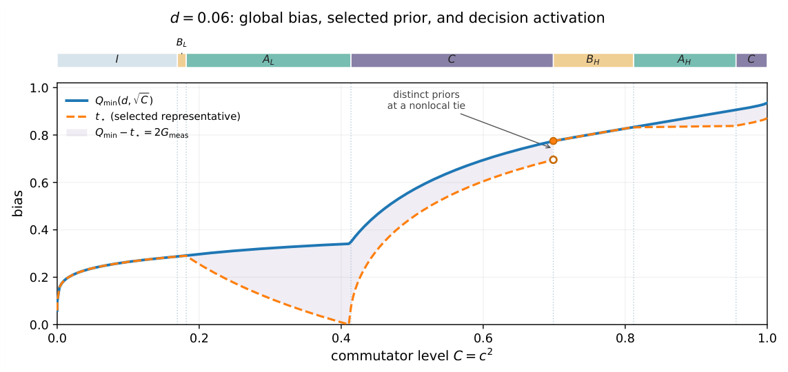

Table 1.
Roadmap of canonical minimizing representatives. The criterion denotes a prior-only optimal decision; means an active measurement improves minimum-error success. Names refer to representatives and need not distinguish physically different sources at continuous attachment points.
Table 1.
Roadmap of canonical minimizing representatives. The criterion denotes a prior-only optimal decision; means an active measurement improves minimum-error success. Names refer to representatives and need not distinguish physically different sources at continuous attachment points.
| Class | Representative geometry | Decision | Physical interpretation |
|---|---|---|---|
| I | Balanced weighted Bloch lengths () | Prior-dominated least-distinguishable source | |
| B | One pure component, threshold | Boundary where measurement becomes useful | |
| A | One pure component, active stationary point | Measurement-active mixed–pure source | |
| C | Both components pure | Pure-state geometric limit |
Table 2.
Proof-dependency roadmap for the global classification. “Exact certificate” means rational/algebraic sign and root assertions over specified domains, not a floating-point phase plot.
Table 2.
Proof-dependency roadmap for the global classification. “Exact certificate” means rational/algebraic sign and root assertions over specified domains, not a floating-point phase plot.
| Logical step | Evidence | Location |
|---|---|---|
| Complete canonical candidate list | Analytic geometry | Theorems 1 and 2; Appendix A |
| Stationary-root and candidate counts | Exact certificates | Theorem 3; Appendix H |
| Ordering and absence of extra transitions | Analytic continuation + exact certificates | Comparisons in Appendices Appendix J.1–Appendix J.4; global synthesis in Appendix J |
| Closed boundaries and equality cases | Analytic endpoint arguments + certified interior order | Appendix K |
Table 3.
Physical information at the isolated global B/A–C equality . The two columns are distinct minimizing ensembles at the same . Along with decision gain and Holevo information, the mean-state purity reveals inequivalent label-blind average states.
Table 3.
Physical information at the isolated global B/A–C equality . The two columns are distinct minimizing ensembles at the same . Along with decision gain and Holevo information, the mean-state purity reveals inequivalent label-blind average states.
| Quantity | One-pure B/A | Two-pure C |
|---|---|---|
| Majority prior p | ||
| Majority Bloch radius | 1 | |
| Minority Bloch radius | 1 | 1 |
| Mean-state radius B | ||
| Mean-state purity | ||
| Decision gain | 0 | |
| Holevo (bit) |
Disclaimer/Publisher’s Note: The statements, opinions and data contained in all publications are solely those of the individual author(s) and contributor(s) and not of MDPI and/or the editor(s). MDPI and/or the editor(s) disclaim responsibility for any injury to people or property resulting from any ideas, methods, instructions or products referred to in the content. |
© 2026 by the authors. Licensee MDPI, Basel, Switzerland. This article is an open access article distributed under the terms and conditions of the Creative Commons Attribution (CC BY) license (http://creativecommons.org/licenses/by/4.0/).
Copyright: This open access article is published under a Creative Commons CC BY 4.0 license, which permit the free download, distribution, and reuse, provided that the author and preprint are cited in any reuse.