

Submitted:
16 November 2026
Posted:
17 November 2026
You are already at the latest version
Abstract
Municipal solid waste incineration (MSWI) represents an important waste-to-energy technology. However, its nitrogen oxide emissions create environmental risks, and accurate NOx prediction remains a challenging task. This challenge arises from variable waste properties, strong nonlinearity in the combustion process, and time-varying operating conditions. Most existing data-driven models are trained under a stationary data distribution. They may produce physically inconsistent predictions, and their performance tends to degrade when process operating conditions shift. This study proposes a physics-informed spatiotemporal graph forecasting framework equipped with drift-triggered continual learning for NOx prediction in MSWI plants. The framework contains three core components. The first is a plant-specific spatiotemporal graph network, which captures spatial coupling across process compartments and temporal dependencies within sensor measurements. The second is a differentiable physical module. It imposes process consistency constraints on the incineration system and steers the network to generate physically plausible predictions. Third, a drift-triggered continual learning mechanism adapts the model online when operating conditions change, while replay and protection strategies reduce catastrophic forgetting and preserve physical and historical consistency. Comparative experiments against state-of-the-art time-series forecasting models verify the effectiveness of the proposed method.
Keywords:
municipal solid waste incineration
; waste-to-energy
; NOx prediction
; spatiotemporal graph neural network
; physics-informed learning
; continual learning
1. Introduction
Municipal solid waste incineration (MSWI) is an important waste-to-energy technology because it can reduce the volume of municipal solid waste while recovering energy for electricity and heat production. However, the combustion process is accompanied by the formation and emission of air pollutants, including nitrogen oxides (NOx) which can cause considerable harm to the environment and human health. Therefore, accurate and timely prediction of NOx concentration is important for emission supervision, reagent control, process optimization, and the safe operation of waste-to-energy plants [1].
The MSWI process is difficult to model because the composition and calorific value of municipal solid waste vary continuously [2]. In addition, the combustion process involves strong nonlinearities, large time delays, multivariable coupling, and interactions among waste feeding, grate movement, primary air, secondary air, furnace temperature, oxygen concentration, and flue-gas treatment [3,4]. The measured NOx concentration is also affected by both the upstream combustion state and the downstream denitrification process, such as selective non-catalytic reduction or selective catalytic reduction [5,6]. Consequently, the relationship between operating variables and NOx emissions is time-dependent and may vary across operating conditions.
Data-driven methods have recently been applied to pollutant and process-variable prediction [7,8,9,10]. For example, Meng et al. developed a brain-inspired modular neural network that integrates task decomposition, self-organizing radial basis function modules, and competitive module selection to improve the accuracy and computational efficiency of NOx prediction in MSWI processes [11]. Qiao et al. proposed an improved interval type-2 fuzzy neural network that combines neighborhood rough-set-based structure determination, adaptive membership functions, and hierarchical parameter learning to enhance NOx prediction accuracy and uncertainty handling in MSWI processes [12]. CNN-LSTM models have been used to extract local feature patterns and temporal dependencies for transient NOx prediction in diesel engines [13]. Graph-based models have also been investigated for transient NOx emission prediction because graph structures can represent relationships among multiple system variables and physical components [14,15,16]. These studies demonstrate the potential of deep neural networks for learning nonlinear emission dynamics [17]. However, most existing models are trained offline on a fixed data distribution. Their predictions may violate material balance and reaction consistency constraints, and their performance tends to degrade under time-varying plant operating conditions.
Physics-informed learning provides a possible solution to the problem of physically inconsistent predictions [18,19]. Instead of relying only on the statistical relationship between input variables and target concentrations, physical information can be introduced through differentiable residuals or conservation constraints [20,21]. Recent studies have demonstrated that physics-informed forecasting models can combine data-driven representation learning with system-level constraints [22,23]. Nevertheless, existing physics-informed forecasting studies have mainly focused on energy systems, production systems, or other engineered processes. A plant-specific framework that represents both the spatial organization of an MSWI plant and the formation, transport, and removal of NOx has not been sufficiently investigated.
Another challenge is that an MSWI plant operates in a nonstationary environment. Temporal changes in the plants operational environment may lead to covariate shift or concept drift, thereby reducing the forecasting accuracy of a static model [24,25]. Continual learning has been proposed to update forecasting models when the data distribution changes while reducing catastrophic forgetting of previously learned knowledge [26,27,28]. For industrial emission prediction, however, model updates must also respect the constraints imposed by online deployment.
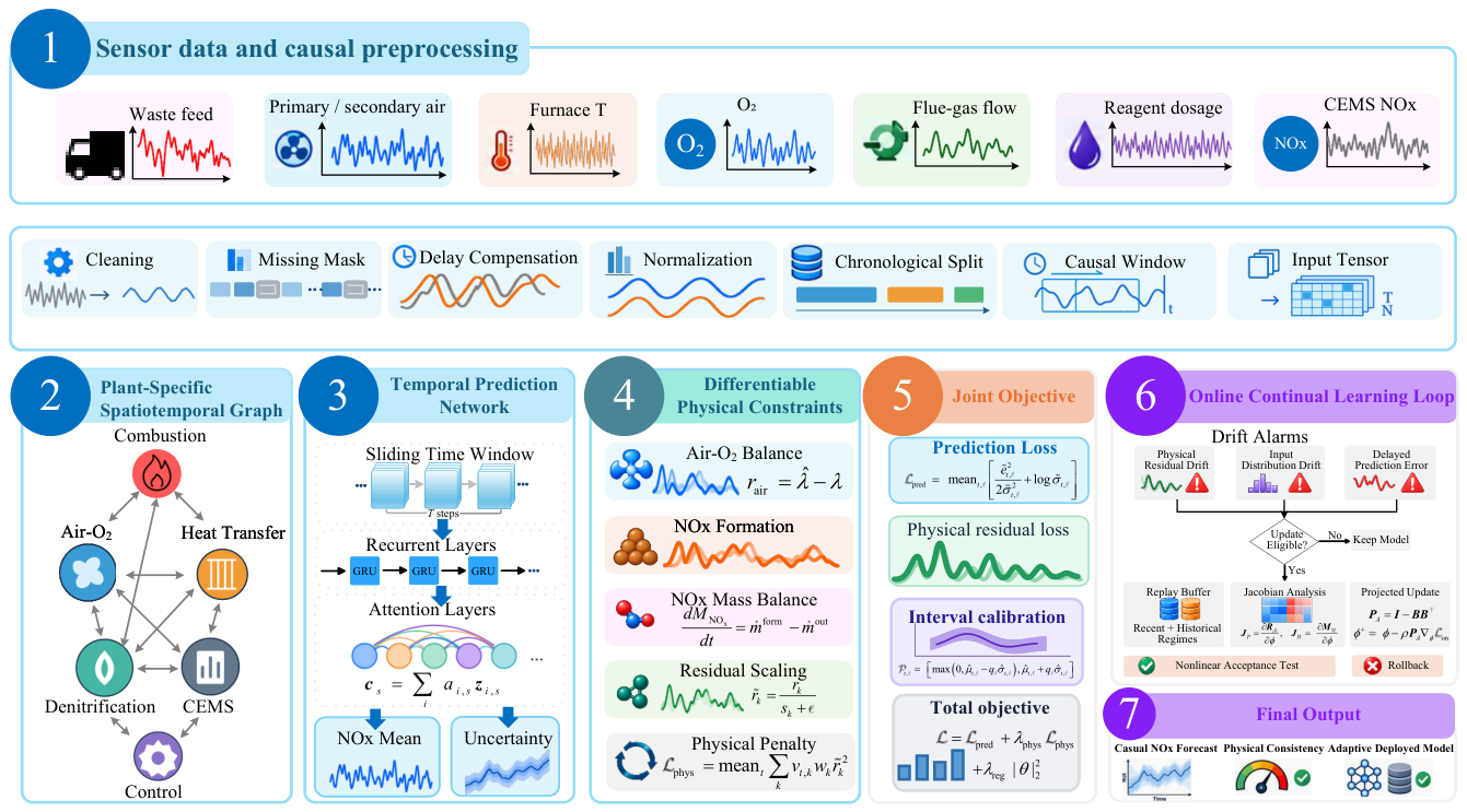
To address these issues, this study proposes a physics-informed spatiotemporal graph forecasting framework with drift-triggered continual learning for NOx prediction in MSWI plants. The proposed method contains three closely related components. First, a plant-specific spatiotemporal graph is constructed to represent gas-flow, solid-feed, heat-transfer, and control relationships among process compartments. A temporal encoder and attention mechanism are then used to extract dynamic dependencies from masked and delayed sensor measurements. Second, a differentiable reduced-order physical module is introduced to impose consistency constraints on oxygen and air balance, fuel-related stoichiometry, NOx formation, denitrification removal, and pollutant mass balance. The physical module works with a probabilistic prediction objective. It outputs NOx concentration estimates together with predictive uncertainty. Third, a drift-triggered continual learning mechanism is designed for online model adaptation. This mechanism detects process shifts by integrating alarms from covariates, physical residuals and delayed prediction errors. In the adaptation phase, only selected trainable directions are updated. The directions linked to physical-residual sensitivities and historical prediction sensitivities are preserved [29]. A replay strategy and a nonlinear acceptance test are additionally adopted. They mitigate catastrophic forgetting and filter out risky parameter updates [30].
The main contributions of this study are as follows: (1) A plant-specific spatiotemporal graph model is developed for representing the coupled combustion, transport, and flue-gas-treatment processes involved in MSWI NOx prediction; (2) The differentiable reduced-order physical module bridges neural predictions and fundamental process conservation rules for incineration; (3) The Drift-triggered continual learning strategy is proposed to adapt the forecasting model to changing operating conditions while protecting physical consistency and historical predictive performance; (4) A causal evaluation protocol is established using chronological data splitting, delayed-label updating, drift detection, replay, ablation analysis, and comparison with non-adaptive baselines.
2. Methods
The framework comprises a physics-informed spatiotemporal graph predictor and a drift-triggered continual learning mechanism. The predictor represents combustion and flue-gas transport through a plant-specific graph and differentiable reduced-order residuals. The continual learner constructs protected directions from physical-residual sensitivities and historical prediction sensitivities in the same trainable parameter space. New data update only the complementary directions, subject to a subsequent nonlinear acceptance check.
2.1. Target Definition
The data used in this study were collected from the No. 1 incineration line of the Lujiashan municipal solid waste incineration plant. The prediction target is the pre-denitrification NOx concentration measured at the economizer outlet. Given the historical operating measurements and available NOx observations, the model predicts the NOx concentration over a future horizon. For a historical window of W samples and a prediction horizon of H samples, the forecasting task is formulated as
where denotes the information available at prediction time t over the historical window, is the plant-specific process graph, and denotes the calibrated physical coefficients. The outputs and represent the predicted mean and conditional standard deviation of the NOx concentration at time , respectively.
Figure 1.
The framework diagram of the proposed method.
2.2. Plant-Specific Spatiotemporal Graph
The graph is with N nodes. Nodes represent instrumented or independently estimable process compartments, such as bed sections, furnace gas volumes, a post-combustion volume, and the boiler gas-path sections up to the target sampling plane. Edges have explicit types:
Gas edges follow documented flue-gas transport, solid edges follow the grate/feed path, heat edges describe justified thermal coupling, and control edges connect actuators to affected compartments. Each edge has a direction, type, estimated delay , and attributes . Node inputs are
where gives time since the last observation and encodes node type and geometry. Global steam flow or load may be supplied as global context. Unobserved temperature, oxygen, or residence-time states are inferred with bounded decoders or supplied by an independently validated estimator. For graph layer , a causal message is
The initial embedding is . The encoder and type-specific message functions are two-layer MLPs with GELU activation. The update function concatenates the node embedding and aggregated message, applies an MLP, and adds a residual connection followed by layer normalization. Layer widths and dropout are reported with the implementation settings. Noninteger delays may be represented by a causal interpolation of buffered states, with interpolation weights identified offline. An edge quality gate uses only observable transport/sensor consistency at time s:
Equation (5) applies when is nonempty; otherwise . Here is the unit-transition Huber function, is a fixed training-derived scale, and prevents complete message suppression. Each must be specified in the edge specification. A global air residual is not arbitrarily assigned to all edges. Input-only gates can modulate the forward computation, but their input-only residuals are not claimed to be differentiable training penalties. Temporal dynamics are represented by
A low-rank adapter is , with rank and flattened parameter vector . Parameters are shared across nodes of the same type. Attention pooling provides context:
The decoder receives and predicts physically bounded local states. Future recurrent inputs comprise previously predicted states, observation masks, and the declared future control scenario.
2.3. Differentiable Physical Residuals
The data-driven predictor is supplemented with a differentiable reduced-order physical module. The purpose of this module is not to reproduce the complete combustion and flue-gas-transport process, but to impose physically meaningful consistency constraints that can be evaluated using the available plant measurements. The physical module considers air–oxygen consistency, fuel-related stoichiometry, NOx formation, transport, and the NOx mass balance within the specified process boundary.
2.3.1. Units, Measured Variables, and Latent States
All measurements are first converted to a common time base and consistent physical units. The oxygen concentration, flue-gas flow rate, waste-feed rate, furnace temperature, and target NOx concentration are denoted by , , , , and , respectively. When a process quantity is not directly measured, it is represented by a latent state estimated by the neural encoder or by a calibrated surrogate relation. The uncertainty of unmeasured or weakly observed quantities is incorporated through confidence weights in the physical residuals. The primary and secondary air flows are denoted by and . The total combustion air flow is calculated as
When a calibrated theoretical air-flow estimate is available, the excess-air ratio is defined as
where is the estimated stoichiometric air requirement and is a small positive constant used for numerical stability. The corresponding air–oxygen consistency residual is
where is the latent excess-air ratio predicted by the physical decoder.
2.3.2. NOx Formation
NOx formation during waste combustion involves the conversion of fuel-bound nitrogen and the oxidation of atmospheric nitrogen. Its net production depends on furnace temperature, oxygen availability, fuel feeding, and mixing conditions. These effects are represented by a reduced-order formation function:
where contains the feeder speed and feeder stroke setting, and denotes the grate speed. The formation term serves as the NOx source in the mass-balance equation described below.
2.3.3. NOx Transport and Mass Balance
Let denote the total NOx mass within the aggregate modeled gas volume, extending from the combustion region to the target sampling plane. The source term represents the net NOx formation within this volume, and the outlet is the target sampling plane. Internal transport between graph compartments cancels in this aggregate balance. External NOx inflow is assumed negligible. Under the negligible-inflow assumption, the reduced-order balance is written as
The outlet mass flow is related to the predicted concentration and flue-gas flow rate:
Using a differentiable time discretization, the pollutant-balance residual at time t is defined as
The physical residual vector for one sample is
where measures consistency between the decoded net formation rate and the reduced-order formation model:
Measured states may replace decoded states when valid observations are available. The predicted concentration and the flue-gas flow at the target sampling plane must use the same wet/dry and reference-volume basis, with an explicit unit conversion when necessary. An oxygen-corrected reporting concentration is converted back to the matching physical concentration before the mass-flow product is evaluated. Because the residuals have different units and numerical ranges, they are normalized using fixed training-set scales. The physical loss is defined as
where is the scale of residual type k, is its prescribed weight, and is a confidence factor determined from sensor quality, missingness, and uncertainty in the corresponding physical relation. Invalid or unavailable measurements are masked rather than imputed as physically valid observations.
2.3.4. Joint Prediction and Physical-Consistency Objective
The supervised prediction loss is combined with the physical loss:
where is the probabilistic NOx forecasting loss, denotes the regularization term, and controls the contribution of the physical constraints.
The physical module therefore acts as a soft constraint. It guides the neural predictor to produce results consistent with the measured process states and NOx mass balance at the target sampling plane. Minor deviations are permitted, which stem from measurement noise, unmeasured waste properties and simplifications in the reduced-order model.
2.4. Offline Training and Predictive Uncertainty
2.4.1. Training Objective
For each prediction horizon, the network outputs the predicted mean and a positive conditional standard deviation:
where ensures numerical stability and is the context representation provided by the spatiotemporal network. The target and prediction outputs are standardized as
where and are the training-set mean and standard deviation. The prediction loss is the Gaussian negative log-likelihood:
where denotes a minibatch of valid training windows. The constant Gaussian term is omitted because it does not affect optimization. Following the joint objective defined above, the offline training loss is
where aggregates the physical residuals defined in the preceding subsection, and . The coefficients and are selected using validation data and remain fixed during offline training. Physical residuals are evaluated in physical units and normalized using training-set scales.
The spatiotemporal backbone, adapters, physical-state decoder, and prediction heads are trained jointly. The model checkpoint is selected according to the validation prediction loss. After offline training, the trained model provides the reference parameters for constructing the protected subspaces used in online adaptation.
2.4.2. Prediction-Interval Calibration
A separate chronological calibration set is used to adjust the prediction intervals after model training and selection. For each horizon ℓ, the normalized absolute prediction errors are
For a nominal miscoverage level , let denote the empirical quantile of the calibration scores at horizon ℓ. The prediction interval is
The calibration quantiles remain fixed during offline evaluation. Interval coverage and width are evaluated separately for each prediction horizon. The offline training and prediction-interval calibration procedures are summarized in Algorithm 1.
| Algorithm 1Offline Training and Interval Calibration |
|
2.5. Continual Learning and Causal Online Adaptation
After offline training, only the adapter parameters are updated online; all other parameters remain fixed. A physical anchor set and a historical replay set retain representative operating samples. The deployed adapter parameters at the beginning of each adaptation event serve as the reference .
2.5.1. Sensitivity-Based Protection
Physical and historical sensitivities are evaluated in the same adapter parameter space:
where contains the normalized, weighted residuals used in , and contains standardized historical prediction means.
The leading right singular vectors of form the physical protection basis . Historical protection directions are extracted from and orthogonalized against to obtain . The combined basis and update projector are
where . The selected ranks leave a nonempty adaptable subspace.
2.5.2. Projected Adaptation
For newly available labeled samples and replay samples , the online objective is
where the prediction and physical losses follow their offline definitions. The physical loss is evaluated on the new and replay samples, and and retain their offline values. The projected update is
where is the step size. The protection basis is fixed within each adaptation event. A nonlinear acceptance test limits deterioration in physical consistency and historical accuracy:
where is the physical loss on and is the standardized prediction mean squared error on valid replay targets. Rejected candidates are retried with a smaller step size; after a limited number of unsuccessful attempts, the reference model remains deployed.
2.5.3. Triggering and Interval Recalibration
Adaptation is triggered by persistent physical-residual or input-distribution alarms, or by increased prediction errors after labels become available:
where is obtained from a training-fitted kernel principal component analysis model, and indicates satisfactory data quality and applicability of the physical constraints. Trigger settings and protection ranks are selected using validation data.
Each forecast is archived before its labels become available. Eligible events reconstruct the protection bases and perform a limited number of projected updates, followed by a cooldown period after acceptance. Prediction intervals are recalibrated using the previously defined normalized-error quantiles on a separate recent calibration buffer with available labels. Updated quantiles apply only to subsequent forecasts. The drift-triggered online adaptation procedure is summarized in Algorithm 2.
| Algorithm 2Drift-Triggered Protected Online Adaptation |
|
3. Experiments and Results
3.1. Experiments Settings
Historical operational data from the Lujiashan Waste-to-Energy Power Plant are adopted for NOx concentration prediction experiments. The sampling interval is 10 s. The dataset covers key operational variables of combustion, air distribution, steam-water and other relevant processes. For missing records, neither interpolation nor backward filling is performed; samples failing to satisfy the validity requirements of input history and prediction targets are discarded. Input variables cover combustion status, air distribution, steam-water conditions, flue gas states, flue gas purification processes, as well as historical NOx measurements available up to the prediction start time. Combustion status variables include furnace temperature, furnace outlet flue gas temperature and grate-related signals. Air distribution variables comprise furnace oxygen content, primary and secondary air flow rates, air pressure and damper opening. Steam-water variables include main steam flow rate.
A direct prediction strategy is adopted in the experiments. Using 60 consecutive minutes of observations up to the current time step as inputs, the NOx concentrations at future horizons of 10, 30 and 60 minutes are predicted separately. Individual models are trained for the three prediction horizons to output single-point predictions at the corresponding future time instants. The dataset is chronologically split into training, validation and test sets at ratios of 60%, 15% and 25%, which are used for model parameter learning, model selection with early stopping, and final performance evaluation, respectively. The target timestamps of training and validation samples maintain a 60-minute gap from the boundary of the subsequent data partition to prevent prediction labels from crossing partition boundaries. All methods are compared using identical test starting points, yielding 13,994 valid test samples.
To mitigate the influence of variable dimensional differences and numerical ranges, inputs and prediction targets are standardized using the median and interquartile range derived from the training set. The transformation parameters obtained from the training set are applied to the validation and test sets. After inverse transformation of model outputs, evaluation metrics are calculated on the original concentration scale.
AdamW optimizer is employed for all models, with an initial learning rate of , weight decay coefficient of , batch size of 128, and a maximum training epoch of 40. Training is terminated early if the validation loss shows no improvement for seven consecutive epochs, and the model parameters corresponding to the minimum validation loss are restored. To reduce computational overhead, one training sample is selected from every two valid prediction starting points in the training set, while all valid samples are retained for the validation and test sets. The experiments are implemented in PyTorch and run on an NVIDIA GeForce RTX 5060 GPU.
Predictive performance was evaluated using root mean square error (RMSE), mean absolute error (MAE), and Mean Absolute Percentage Error (MAPE).
where and denote the measured value and predicted value, respectively, and N is the number of evaluation samples. Smaller values of these metrics correspond to lower prediction errors.
3.2. Model Prediction Performance Analysis
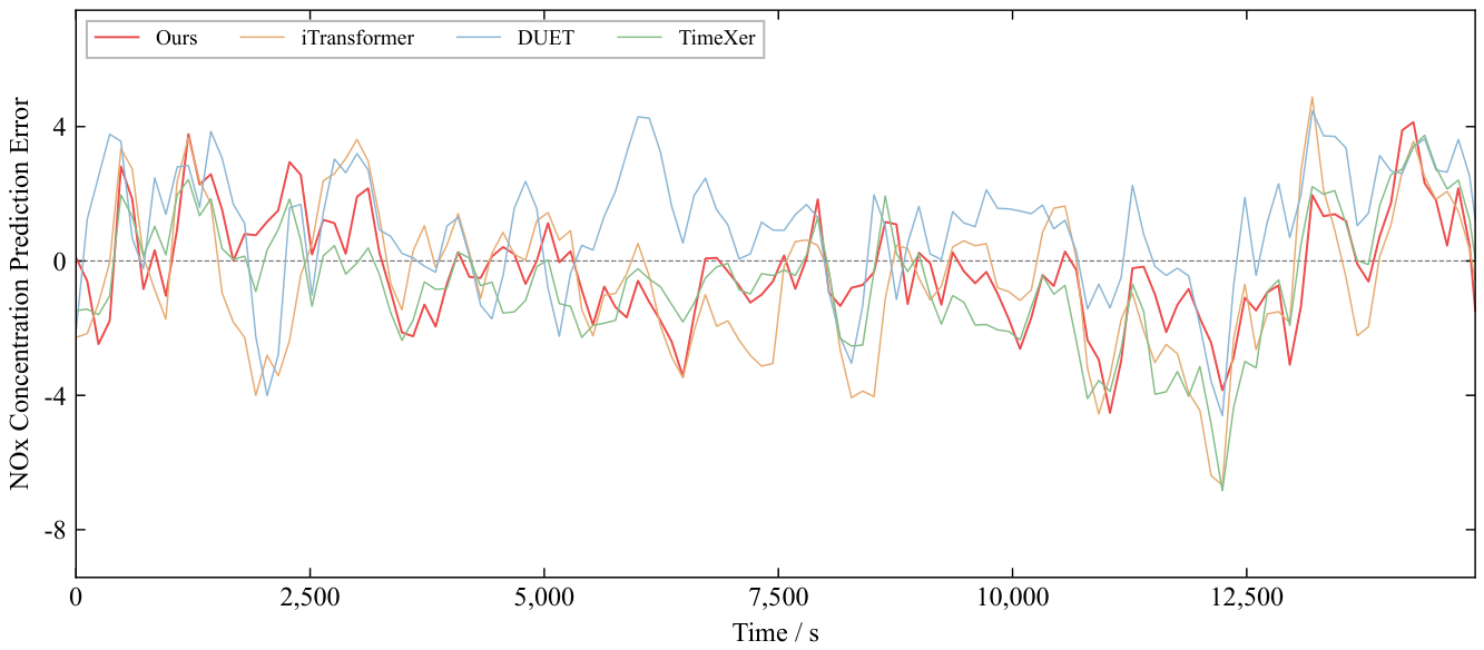
Three state-of-the-art models including iTransformer, DUET and Timexer are adopted for comparison with our method under identical experimental settings. Figure 2 to 7 show the prediction and error curves for different models. As shown in the figures, under the three prediction horizons, the prediction curve of our method achieves the optimal performance in both trend and magnitude compared with the other three approaches. Particularly for segments where the raw data fluctuate violently, the proposed approach is capable of detecting trend variations promptly and following them closely.
Figure 3.
Prediction errors of different models under the 10-min prediction horizon.
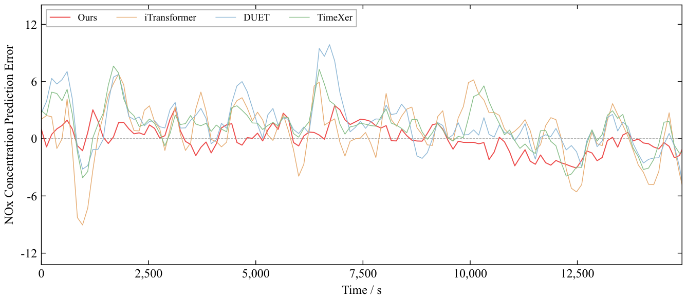
Figure 4.
Prediction results of different models under the 30-min prediction horizon.
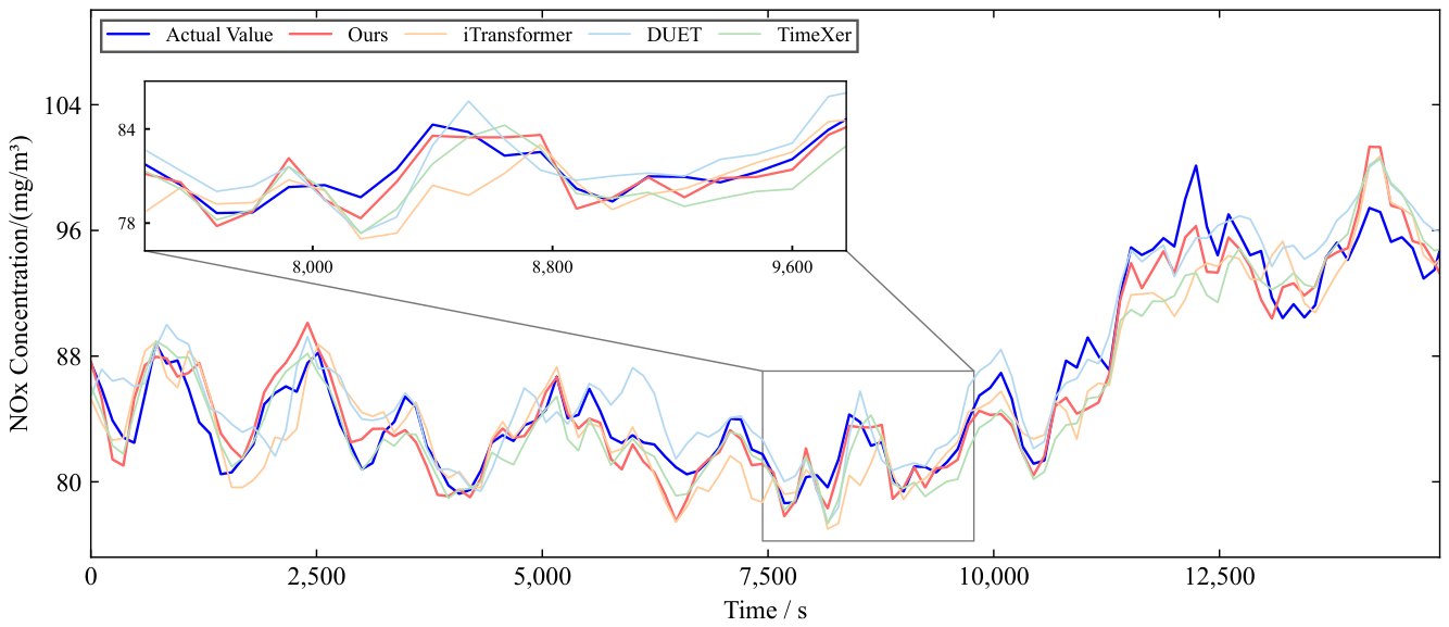
Figure 5.
Prediction errors of different models under the 30-min prediction horizon.
Three performance metrics of models under the three prediction horizons are summarized in Table 1. As can be seen from the table, the proposed method achieves the lowest values of the three evaluation metrics under all three prediction horizons. Moreover, the prediction errors of all models increase to varying degrees as the prediction horizon grows, while the proposed method exhibits a smaller error increment and stronger robustness for long-horizon forecasting.
To better show the prediction performance of each model, Figure 8 uses box plots to display the distribution of their prediction errors. The box plot results show that, compared to other methods, the proposed method has lower overall absolute errors across different prediction timeframes, with a more concentrated distribution, and can better control large prediction deviations, showing better prediction accuracy and stability.
To further evaluate the performance of the proposed method under different load levels of the system, prediction experiments were conducted for rising, falling, and relatively stable power generation load conditions, respectively. As shown in Figure 9, under falling, stable, and rising load conditions, the prediction results of this method maintained good agreement with the measured nitrogen oxide concentrations. During load decline, the proposed method successfully captured the overall downward trend in concentration, and its absolute error distribution was more concentrated compared to the benchmark model, although the median error of the DUET model was slightly lower. Under steady-state load conditions, the advantages of the proposed method were most pronounced: it exhibited a lower median absolute error and a narrower interquartile range, whereas the benchmark method showed greater deviations or higher error dispersion. When the load increases, this method can track the rising concentration trend, with errors remaining at a low level and exhibiting a concentrated distribution. Overall, the above results indicate that this method possesses stable and excellent predictive accuracy under various load conditions, with generally lower error dispersion, making it suitable for variable operating conditions.
Table 2 compares the forecasting performance under decreasing, steady, and increasing load conditions for the three prediction horizons. Under steady load, the proposed method outperforms all competing methods consistently across all horizons and metrics. It achieves an RMSE reduction of 19.43%-28.08% compared with the best baseline at each horizon. Under increasing load, its advantage is particularly pronounced at the 60-min horizon, where RMSE and MAE are reduced by 34.80% and 39.07%, respectively, compared with the strongest corresponding baselines. Under decreasing load, the proposed method achieves the lowest errors at the 10- and 60-min horizons, while DUET performs slightly better at 30 min. Overall, these results support the effectiveness of the proposed framework across different load conditions, while indicating that its relative advantage varies with the operating condition and prediction horizon.
Figure 6.
Prediction results of different models under the 60-min prediction horizon.
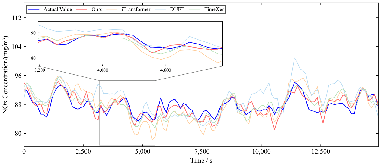
Figure 7.
Prediction errors of different models under the 60-min prediction horizon.
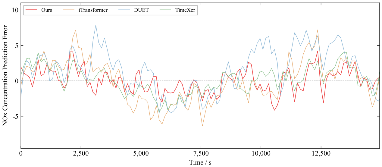
Figure 8.
Boxplot of prediction errors across models under different prediction horizons.
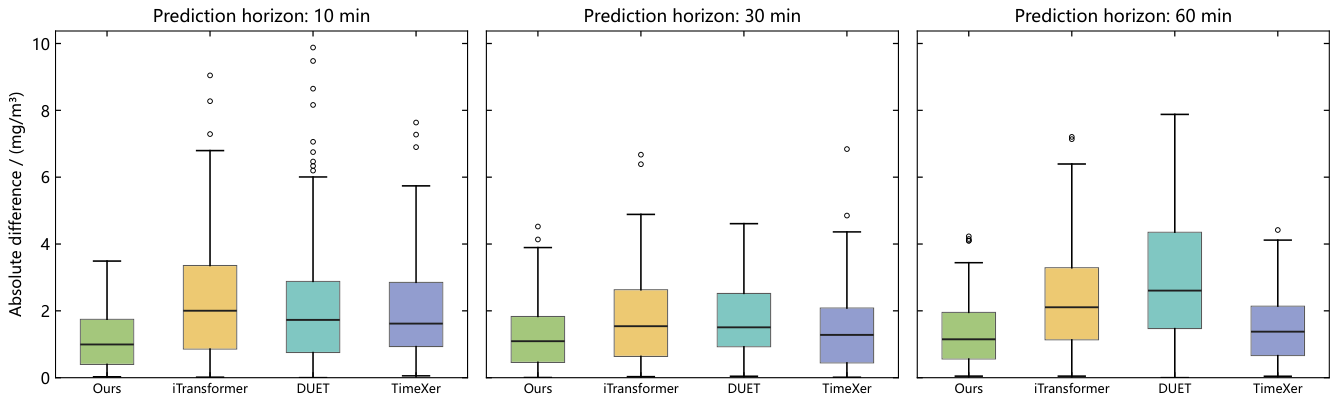
Figure 9.
Comparison of Prediction Performance under 10-min Prediction Horizon of Different Models under Various Load Levels. (a) Prediction performance of different models under decreasing load. (b) Prediction errors distribution for different models under decreasing load. (c) Comparison of prediction performance of different models under steady load. (d) Prediction errors distribution for different models under steady load. (e) prediction performance of different models under increasing load. (f) Distribution of prediction errors for different models under increasing load.
Figure 9.
Comparison of Prediction Performance under 10-min Prediction Horizon of Different Models under Various Load Levels. (a) Prediction performance of different models under decreasing load. (b) Prediction errors distribution for different models under decreasing load. (c) Comparison of prediction performance of different models under steady load. (d) Prediction errors distribution for different models under steady load. (e) prediction performance of different models under increasing load. (f) Distribution of prediction errors for different models under increasing load.
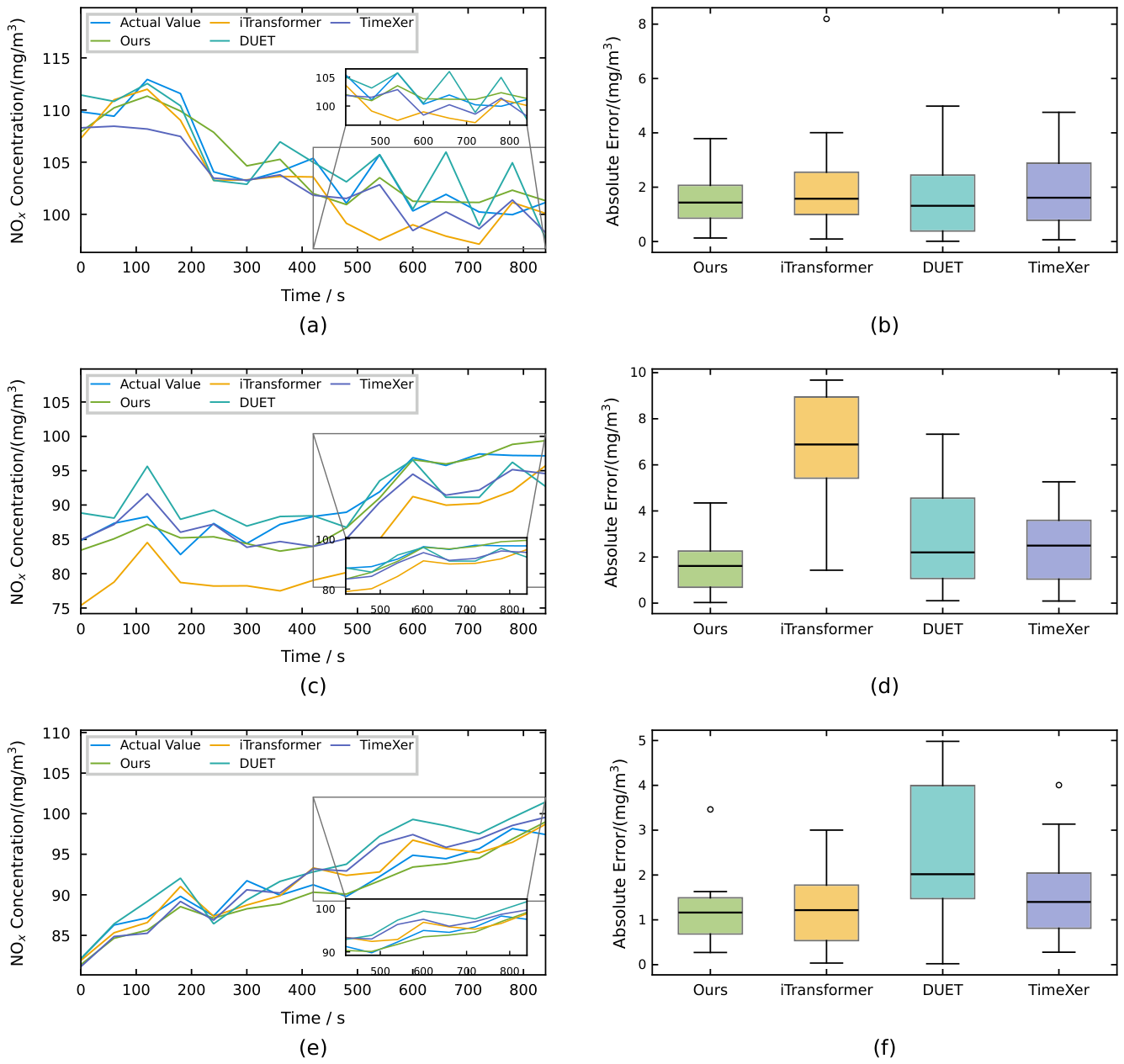

Table 1.
Evaluation Index of Different Models for the Forecasting Task
| Model | 10 minutes | 30 minutes | 60 minutes | ||||||
|---|---|---|---|---|---|---|---|---|---|
| RMSE | MAE | MAPE | RMSE | MAE | MAPE | RMSE | MAE | MAPE | |
| Ours | 1.44 | 1.16 | 1.35 | 1.62 | 1.28 | 1.47 | 1.67 | 1.35 | 1.55 |
| iTransformer | 3.02 | 2.36 | 2.77 | 2.22 | 1.78 | 2.04 | 2.92 | 2.42 | 2.78 |
| DUET | 3.01 | 2.22 | 2.71 | 2.07 | 1.73 | 2.01 | 3.45 | 2.88 | 3.29 |
| TimeXer | 2.58 | 2.06 | 2.46 | 1.91 | 1.47 | 1.67 | 1.88 | 1.55 | 1.77 |
The best results have been bold.
Table 2.
Comparison of Forecasting Performance under Different Load Conditions
| Model | Horizon | Decreasing Load | Steady load | Increasing load | ||||||
|---|---|---|---|---|---|---|---|---|---|---|
| RMSE | MAE | MAPE | RMSE | MAE | MAPE | RMSE | MAE | MAPE | ||
| Our | 10 | 1.86 | 1.55 | 1.47 | 2.10 | 1.70 | 1.91 | 1.40 | 1.19 | 1.30 |
| 30 | 2.60 | 2.03 | 2.73 | 2.53 | 2.21 | 2.36 | 1.22 | 1.05 | 1.18 | |
| 60 | 1.78 | 1.55 | 1.70 | 2.04 | 1.70 | 1.28 | 2.23 | 1.84 | 1.51 | |
| iTransformer | 10 | 2.84 | 2.10 | 2.01 | 3.34 | 2.74 | 3.53 | 1.48 | 1.19 | 1.29 |
| 30 | 4.74 | 3.86 | 5.14 | 3.14 | 2.67 | 3.09 | 1.61 | 1.32 | 1.49 | |
| 60 | 1.85 | 1.58 | 1.73 | 2.61 | 2.44 | 1.53 | 3.42 | 3.34 | 3.69 | |
| DUET | 10 | 2.23 | 1.67 | 1.62 | 3.63 | 2.90 | 3.22 | 2.82 | 2.38 | 2.57 |
| 30 | 2.45 | 2.01 | 2.72 | 3.70 | 3.09 | 3.32 | 2.81 | 2.26 | 2.58 | |
| 60 | 2.91 | 2.12 | 2.53 | 2.93 | 2.75 | 1.56 | 3.81 | 3.02 | 2.49 | |
| TimeXer | 10 | 2.36 | 1.92 | 1.81 | 2.92 | 2.43 | 2.65 | 1.88 | 1.58 | 1.72 |
| 30 | 2.66 | 2.29 | 3.13 | 3.73 | 3.27 | 3.50 | 2.40 | 1.99 | 2.23 | |
| 60 | 2.00 | 1.75 | 1.92 | 2.92 | 2.62 | 1.98 | 4.70 | 3.94 | 3.28 | |
The best results have been bold. The second-best results have been underlined.
3.3. Ablation Study of Model Components
To comprehensively quantify the individual contribution of each component within the proposed model, we design four sets of ablation experiments, with the results summarized in Table II. The full end-to-end model is retained as the control group, while variants G1-G4 correspond to ablated model configurations obtained by removing one single component from the complete pipeline, respectively.
Table 3 presents the quantitative analysis results across all ablation groups. The analysis yields the following key findings:
- 1.
- G1(w/o SGM): Removing spatiotemporal graph modeling increases the 10-min RMSE from 1.44 to 5.32 and MAE from 1.16 to 3.56. Similar performance degradation occurs at the longer prediction horizons, with RMSE reaching 6.41 at 60 min. These results support the importance of representing process interactions and temporal dynamics for accurate NOx prediction.
- 2.
- G2(w/o PCC): Without physical consistency constraints, the 10-min RMSE increases to 5.03, while the 60-min RMSE and MAPE rise to 6.23 and 4.81%, respectively. This indicates that physical regularization contributes to prediction accuracy by incorporating process knowledge into model learning.
- 3.
- G3(w/o CLUA): Removing continual learning and update acceptance produces the largest errors at the 60-min horizon, with RMSE, MAE, and MAPE reaching 6.49, 4.57, and 5.25%, respectively. This suggests that the combined adaptation and acceptance mechanism is particularly important for maintaining predictive performance at longer horizons under the evaluated conditions.
- 4.
- G4(w/o DTAM): Removing drift-triggered adaptation mechanism increases the 10-min RMSE to 4.92 and the 60-min MAE to 4.32. The consistent degradation across prediction horizons supports the contribution of drift-aware update scheduling to maintaining forecasting accuracy.
Table 3.
Ablation Study of Model Components
| Group | 10 minutes | 30 minutes | 60 minutes | ||||||
|---|---|---|---|---|---|---|---|---|---|
| RMSE | MAE | MAPE | RMSE | MAE | MAPE | RMSE | MAE | MAPE | |
| Full Model | 1.44 | 1.16 | 1.35 | 1.62 | 1.28 | 1.47 | 1.67 | 1.35 | 1.55 |
| w/o SGM | 5.32 | 3.56 | 4.14 | 5.83 | 3.79 | 4.35 | 6.41 | 4.28 | 4.91 |
| w/o PCC | 5.03 | 3.21 | 3.74 | 5.39 | 3.47 | 3.99 | 6.23 | 4.19 | 4.81 |
| w/o CLUA | 5.29 | 3.58 | 4.17 | 5.73 | 4.10 | 4.71 | 6.49 | 4.57 | 5.25 |
| w/o DTAM | 4.92 | 3.23 | 3.76 | 5.01 | 3.81 | 4.38 | 6.17 | 4.32 | 4.96 |
The best results have been bold. SGM denotes spatiotemporal graph modeling, PCC refers to physical consistency constraints,
CLUA represents continual learning and update acceptance, and DTAM corresponds to the drift-triggered adaptation
mechanism.
Overall, the full model achieves the lowest RMSE, MAE, and MAPE across all three prediction horizons, demonstrating the complementary contributions of graph modeling, physical constraints, continual adaptation, and drift-triggered updating. These findings support the effectiveness of their integration for accurate multihorizon NOx forecasting.
3.4. Robustness and Stability Verification
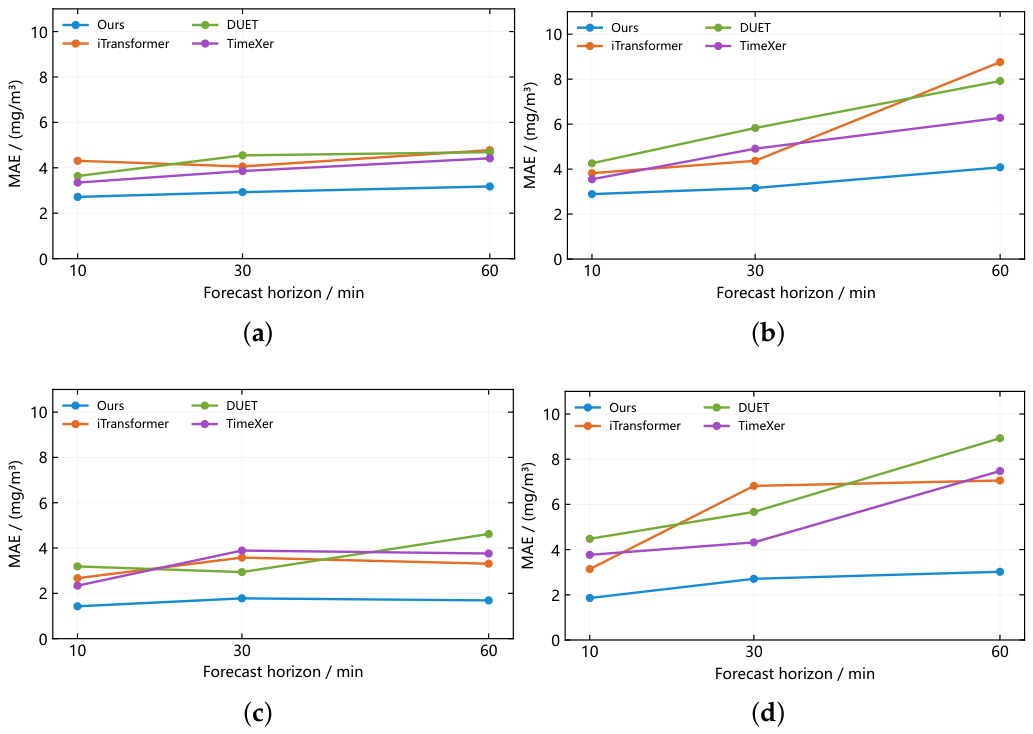
MSWI is a process that constantly faces frequent and complex disturbances, including changes in waste composition, sensor malfunctions, and environmental changes. To verify the robustness and stability of the proposed model, we introduce four types of perturbations, including Gaussian noise, Brownian noise, random missing values, and continuous missing values, into the datasets to simulate the above working conditions. We compare our model with other baselines to evaluate its performance under noisy environments.
Figure 10 presents the prediction errors of several models under four perturbation conditions across three prediction horizons. As illustrated in the figure, the proposed method achieves the lowest prediction errors across three prediction horizons under all four perturbation conditions when compared with other approaches. In addition, the prediction errors of other models accumulate as the prediction horizon increases. By contrast, our model maintains strong stability even for long-horizon prediction tasks.
4. Discussion
The experimental results indicate that the proposed framework improves NOx forecasting performance. Compared with the evaluated baselines, the proposed method yields lower overall prediction errors for different forecasting horizons. It also maintains competitive performance under different load conditions. The ablation results further support the contributions of the main components. Together, these findings suggest that integrating process knowledge with adaptive learning offers an effective approach to forecasting under varying MSWI operating conditions.
Several limitations should be acknowledged. First, the evaluation is based on data from a single incineration line, which limits conclusions regarding generalization to other plants and operating environments. Second, the reduced-order physical constraints rely on the quality of field measurements and state estimation. Accordingly, their applicability changes with the waste properties and operating scenarios. Third, the current prediction metrics and component-level ablations are insufficient to fully validate the model desirable properties throughout online adaptation. The protection provided by the adaptation mechanism also depends on the representativeness of the anchor and replay samples.
Our next research will extend the evaluation to longer operating periods and multiple incineration lines to examine generalization and transferability. Further efforts will focus on improving physical-module calibration, quantifying the effects of individual protection mechanisms, and evaluating predictive uncertainty and robustness under realistic disturbances. Computational efficiency and long-term online performance will also be investigated.
5. Conclusions
This study developed a physics-informed spatiotemporal graph forecasting framework with drift-triggered continual learning for predicting NOx concentrations arising from municipal solid waste incineration for power generation. The framework combines a plant-specific process graph, differentiable reduced-order physical constraints, and online adapter updates guided by physical-residual and historical prediction sensitivities. A nonlinear acceptance procedure further evaluates candidate updates before deployment.
Results demonstrate that the proposed method achieves superior overall NOx prediction accuracy across all horizons. Experiments under decreasing, steady, and increasing load conditions demonstrated broadly competitive performance, while the ablation results supported the contributions of graph modeling, physical regularization, and continual adaptation. These findings indicate that integrating process knowledge with constrained online learning is a promising approach to industrial NOx forecasting. Future work will explore the integration of the proposed framework into emission control and operational optimization in municipal solid waste incineration power generation.
Author Contributions
A short paragraph specifying our individual contributions is provided as follows: “Conceptualization, Yuntao Tang and Haixu Ding; methodology, Yuntao Tang and Tao Yu; software, Guangwei Chen and Tao Yu; validation, Yuntao Tang, Tao Yu and Haixu Ding; formal analysis, Guangwei Chen; investigation, Junfei Qiao; resources, Junfei Qiao; data curation, Haixu Ding and Yuntao Tang; writing—original draft preparation, Yuntao Tang; writing—review and editing, Haixu Ding and Guangwei Chen; visualization, Tao Yu; supervision, Junfei Qiao; project administration, Haixu Ding; funding acquisition, Junfei Qiao. All authors have read and agreed to the published version of the manuscript.”
Funding
This work was supported in part by the National Natural Science Foundation of China under Grant 62503021, in part by the China Postdoctoral Science Foundation under Grant GZC20251167 and Grant 2025M781625, in part by the Beijing Postdoctoral Research Foundation under Grant 2025-ZZ-38.
Data Availability Statement
The datasets generated and analyzed in this study are available from the corresponding author upon reasonable request.
Conflicts of Interest
The authors declare no conflicts of interest.
Abbreviations
The following abbreviations are used in this manuscript:
| MSWI | Municipal Solid Waste Incineration |
| NOx | Nitrogen Oxides |
| RMSE | Root Mean Square Error |
| MAE | Mean Absolute Error |
| MAPE | Mean Absolute Percentage Error |
References
- Tao, J.; Li, Z.; Chen, C.; Liang, R.; Wu, S.; Lin, F.; Cheng, Z.; Yan, B.; Chen, G. Intelligent technologies powering clean incineration of municipal solid waste: A system review. Sci. Total Environ. 2024, 935, 173082. [Google Scholar] [CrossRef] [PubMed]
- Zhuang, J.; Tang, J.; Aljerf, L. Comprehensive review on mechanism analysis and numerical simulation of municipal solid waste incineration process based on mechanical grate. Fuel 2022, 320, 123826. [Google Scholar] [CrossRef]
- Magnanelli, E.; Tranås, O. L.; Carlsson, P.; Mosby, J.; Becidan, M. Dynamic modeling of municipal solid waste incineration. Energy 2020, 209, 118426. [Google Scholar] [CrossRef]
- Li, Z.; Fan, T. W.; Lun, M. S.; Li, Q. Optimization of municipal solid waste incineration for low-NOx emissions through numerical simulation. Sci. Rep. 2024, 14, 19309. [Google Scholar] [CrossRef] [PubMed]
- Hu, Z.; Jiang, E.; Ma, X. Numerical simulation on operating parameters of SNCR process in a municipal solid waste incinerator. Fuel 2019, 245, 160–173. [Google Scholar] [CrossRef]
- Yan, Q.; Yang, R.; Zhang, Y.; Umar, A.; Huang, Z.; Wang, Q. A comprehensive review on selective catalytic reduction catalysts for NOx emission abatement from municipal solid waste incinerators. Environ. Prog. Sustain. Energy 2016, 35, 1061–1069. [Google Scholar] [CrossRef]
- Duan, H.; Meng, X.; Tang, J.; Qiao, J. Prediction of NOx concentration using modular long short-term memory neural network for municipal solid waste incineration. Chin. J. Chem. Eng. 2023, 56, 46–57. [Google Scholar] [CrossRef]
- Duan, H.; Meng, X.; Tang, J.; Qiao, J. NOx emissions prediction for MSWI process based on dynamic modular neural network. Expert Syst. With Appl. 2024, 238, 122015. [Google Scholar] [CrossRef]
- Wang, R.; Li, F.; Yan, A. Modular stochastic configuration network based prediction model for NOx emissions in municipal solid waste incineration process. Eng. Appl. Artif. Intell. 2024, 127, 107315. [Google Scholar] [CrossRef]
- Wang, R.; Yan, A. R-SCN based model predictive control for NOx emissions of MSWI process. 2023 CAA Symposium on Fault Detection, Supervision and Safety for Technical Processes (SAFEPROCESS), 2023; pp. 1–5. [Google Scholar]
- Meng, X.; Tang, J.; Qiao, J. NOx emissions prediction with a brain-inspired modular neural network in municipal solid waste incineration processes. IEEE Trans. Ind. Inform. 2021, 18, 4622–4631. [Google Scholar] [CrossRef]
- Qiao, J.; Sun, Z.; Meng, X. A comprehensively improved interval type-2 fuzzy neural network for NOx emissions prediction in MSWI process. IEEE Trans. Ind. Inform. 2023, 19, 11286–11297. [Google Scholar] [CrossRef]
- Shen, Q.; Wang, G.; Wang, Y.; Zeng, B.; Yu, X.; He, S. Prediction model for transient NOx emission of diesel engine based on CNN-LSTM network. Energies 2023, 16, 5347. [Google Scholar] [CrossRef]
- Li, Y.; Yu, R.; Shahabi, C.; Liu, Y. Diffusion convolutional recurrent neural network: Data-driven traffic forecasting. arXiv 2017, arXiv:1707.01926. [Google Scholar]
- Wu, Z.; Pan, S.; Long, G.; Jiang, J.; Zhang, C. Graph wavenet for deep spatial-temporal graph modeling. arXiv 2019, arXiv:1906.00121. [Google Scholar]
- Chen, Y.; Liang, C.; Liu, D.; Niu, Q.; Miao, X.; Dong, G.; Li, L.; Liao, S.; Ni, X.; Huang, X. Embedding-graph-neural-network for transient NOx emissions prediction. Energies 2022, 16, 3. [Google Scholar] [CrossRef]
- Wu, Z.; Pan, S.; Long, G.; Jiang, J.; Chang, X.; Zhang, C. Connecting the dots: Multivariate time series forecasting with graph neural networks. In Proceedings of the 26th ACM SIGKDD International Conference on Knowledge Discovery & Data Mining, 2020; pp. 753–763. [Google Scholar]
- Karpatne, A.; Atluri, G.; Faghmous, J. H.; Steinbach, M.; Banerjee, A.; Ganguly, A.; Shekhar, S.; Samatova, N.; Kumar, V. Theory-guided data science: A new paradigm for scientific discovery from data. IEEE Trans. Knowl. Data Eng. 2017, 29, 2318–2331. [Google Scholar] [CrossRef]
- Karniadakis, G. E.; Kevrekidis, I. G.; Lu, L.; Perdikaris, P.; Wang, S.; Yang, L. Physics-informed machine learning. Nat. Rev. Phys. 2021, 3, 422–440. [Google Scholar] [CrossRef]
- Raissi, M.; Perdikaris, P.; Karniadakis, G. E. Physics-informed neural networks: A deep learning framework for solving forward and inverse problems involving nonlinear partial differential equations. J. Comput. Phys. 2019, 378, 686–707. [Google Scholar] [CrossRef]
- Jagtap, A. D.; Kharazmi, E.; Karniadakis, G. E. Conservative physics-informed neural networks on discrete domains for conservation laws: Applications to forward and inverse problems. Comput. Methods Appl. Mech. Eng. 2020, 365, 113028. [Google Scholar] [CrossRef]
- Liu, W.; Pyrcz, M. J. Physics-informed graph neural network for spatial-temporal production forecasting. Geoenergy Sci. Eng. 2023, 223, 211486. [Google Scholar] [CrossRef]
- Sayghe, A.; Mousa, M. A.; Batiyah, S.; Husawi, A.; Almuwallad, M. GridFM: A physics-informed foundation model for multi-task energy forecasting using real-time NYISO data. Energies 2026, 19, 357. [Google Scholar] [CrossRef]
- Gama, J.; Žliobaitė, I.; Bifet, A.; Pechenizkiy, M.; Bouchachia, A. A survey on concept drift adaptation. ACM Comput. Surv. 2014, 46, 1–37. [Google Scholar] [CrossRef] [PubMed]
- Lu, J.; Liu, A.; Dong, F.; Gu, F.; Gama, J.; Zhang, G. Learning under concept drift: A review. IEEE Trans. Knowl. Data Eng. 2018, 31, 2346–2363. [Google Scholar] [CrossRef]
- Besnard, Q.; Ragot, N. Continual learning for time series forecasting: A first survey. Eng. Proc. 2024, 68, 49. [Google Scholar] [CrossRef]
- Kirkpatrick, J.; Pascanu, R.; Rabinowitz, N.; Veness, J.; Desjardins, G.; Rusu, A. A.; Milan, K.; Quan, J.; Ramalho, T.; Grabska-Barwinska, A.; et al. Overcoming catastrophic forgetting in neural networks. Proc. Natl. Acad. Sci. 2017, 114, 3521–3526. [Google Scholar] [CrossRef] [PubMed]
- Lopez-Paz, D.; Ranzato, M.-A. Gradient episodic memory for continual learning. Adv. Neural Inf. Process. Syst. 2017, 30. [Google Scholar]
- Farajtabar, M.; Azizan, N.; Mott, A.; Li, A. Orthogonal gradient descent for continual learning. International Conference on Artificial Intelligence and Statistics, 2020; pp. 3762–3773. [Google Scholar]
- Saha, G.; Garg, I.; Roy, K. Gradient projection memory for continual learning. arXiv 2021, arXiv:2103.09762. [Google Scholar]
Figure 2.
Prediction results of different models under the 10-min prediction horizon.
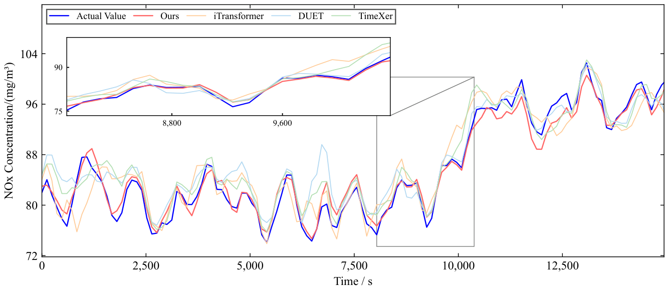
Figure 10.
Model Performance Comparison Across Different Perturbation Scenarios. (a) Gaussian noise. (b) Brownian noise. (c) Random missingness. (d) Continuous missingness.
Figure 10.
Model Performance Comparison Across Different Perturbation Scenarios. (a) Gaussian noise. (b) Brownian noise. (c) Random missingness. (d) Continuous missingness.
Disclaimer/Publisher’s Note: The statements, opinions and data contained in all publications are solely those of the individual author(s) and contributor(s) and not of MDPI and/or the editor(s). MDPI and/or the editor(s) disclaim responsibility for any injury to people or property resulting from any ideas, methods, instructions or products referred to in the content. |
© 2026 by the authors. Licensee MDPI, Basel, Switzerland. This article is an open access article distributed under the terms and conditions of the Creative Commons Attribution (CC BY) license (http://creativecommons.org/licenses/by/4.0/).
Copyright: This open access article is published under a Creative Commons CC BY 4.0 license, which permit the free download, distribution, and reuse, provided that the author and preprint are cited in any reuse.