

Submitted:
17 November 2026
Posted:
17 November 2026
You are already at the latest version
Abstract
Advanced clay models capture anisotropy and stress history but are hard to calibrate and implement; compact bounding-surface models are practical but miss the anisotropic undrained response. This study distils knowledge from an advanced model into a compact one that remains a plasticity model. The teacher is MIT-S1 with published Boston Blue Clay parameters, whose own plastic strains are recorded; the student is the AJOP-T bounding-surface model with a fabric variable, written in a differentiable framework. Two closed forms are learned: a kinematic, fabric-dependent Nova-type plastic potential, identified by an inverse dilatancy analysis, and the exponent of the bounding plastic modulus. Splits, selection rule and pass criteria were fixed before fitting. Trained on 96 paths and selected by validation loss, the student reproduced all 32 held-out undrained paths with normalized error below 10%, predicted undrained strength within 10% for 94% of isotropic and 100% of K0 test paths, with a mean flow-direction mismatch of 7.8° against the teacher. Extension of K0 clay was not learned from compression data; two extension tests reduce the strength error on 17 unseen paths from about 47% to 11%. Trained only where the teacher matches laboratory data, a student predicted the unseen isotropic strength of Lower Cromer Till with a mean error of 12%, against 20% for the teacher. Trained on twelve synthetic MIT-S1 clays, it reproduced five laboratory clays about as well as the single-teacher student.
Keywords:
knowledge extraction
; teacher–student distillation
; plastic potential
; bounding-surface plasticity
; clay anisotropy
; differentiable simulation
; MIT-S1
; symbolic model discovery
1. Introduction
Soft clay controls the design of embankments, excavations, foundations and storage reservoirs [1,2,3]. Its undrained strength depends on how it was consolidated and in which direction it is sheared [1,4]. K0-consolidated clay is much weaker in triaxial extension than in compression [4,5]. A model that ignores this anisotropy can misjudge strength by tens of percent [4,6].
Advanced effective-stress models capture these effects. MIT-E3 and MIT-S1 reproduce the anisotropic, OCR-dependent response of Boston Blue Clay (BBC) closely [4,7,8,9]. Other anisotropic models, such as S-CLAY1 and SANICLAY, add rotational hardening to critical-state plasticity [5,6,10,11]. The cost is high. MIT-S1 has 13 clay parameters, some from non-standard tests [8,12]. Its integration needs reversal memory and careful intersection logic [9,13,14]. Few practitioners can calibrate or implement such a model.
Compact bounding-surface models are the practical alternative [15,16,17]. Our group has developed one such line. It started from the arc compression equation of the simplified silty sand model [18], was refined for settlement analysis [19], and was embedded in a teardrop bounding surface with transformed stress [20,21,22]. AJOP-T then made the compression slope a smooth, differentiable function of the hardening variable [23]. Fractional extensions studied how geometry, flow and compression interact [24,25,26,27]. Robust integration was addressed separately [14]. These models are easy to calibrate and fast to run [2,3,19]. However, like most compact models, they do not reproduce the anisotropic undrained response of an advanced model.
Machine learning (ML) offers a way to close this gap. Neural networks have modelled material behaviour for three decades [28,29]. Recurrent networks now learn path-dependent plasticity [30,31]. Data-driven solvers can even bypass the constitutive model [32]. For soils, reviews document rapid growth of such models [33], and applications range from stress–strain curves to consolidation and slope surrogates [34,35,36]. Most of these models are black boxes. They predict well inside their training range, but an engineer cannot inspect them, transfer them to another code, or check them against mechanics [33,37,38].
Physics-informed learning reduces this problem. Some methods enforce thermodynamics [39,40]. Others learn a yield function or a hardening law inside a plasticity structure [41,42,43], or constrain the network architecture itself [44,45,46,47,48]. Another line seeks interpretable equations directly. Sparse regression and symbolic regression recover closed-form laws from data [49,50,51]. Symbolic distillation of a trained network is a related route [52]. In knowledge distillation, a compact student learns from a large teacher [53,54]. Recent work asks which knowledge actually transfers in such schemes [55], and how knowledge can be extracted from simulators [56,57,58].
These strands have not been combined for clay plasticity. Three gaps remain. First, distillation has not been used between two plasticity models, where the teacher is an advanced model and the student is a compact model that must stay a plasticity model [33,53]. Second, learned constitutive components are rarely checked against the teacher’s internal quantities, such as its plastic strains; agreement of stress paths is usually taken as enough [30,31,41]. Third, reports seldom state what fails: unseen loading modes, training pathologies and parameter non-uniqueness are often left out [59,60].
This paper addresses these gaps. The teacher is MIT-S1 with the published BBC parameters [8]. The student is AJOP-T with a scalar fabric variable [20,23]. Only two mechanisms of the student may learn: the plastic potential g and, from stage S7, the exponent of the bounding plastic modulus with the starting fabric. g is the main target because it sets the dilatancy, and in undrained shear the dilatancy sets the effective stress path and the strength [10,61,62]. Every other part of the student keeps its form. The result is still a bounding-surface model, now with a closed-form, differentiable g and a closed-form hardening exponent.
The novelty lies in six points. (i) This is, to our knowledge, the first teacher–student extraction of a plastic potential between two clay plasticity models. (ii) The teacher’s own plastic strains are recorded, so the learned flow is checked against the teacher’s flow, not only against its stresses. (iii) A neural potential trained end-to-end failed, and an inverse dilatancy analysis pointed to a closed form; the paper reports both. (iv) The extracted potential is a fabric-dependent Nova-type law that reproduces held-out paths and the teacher’s flow direction. (v) The limits are measured, not assumed: a held-out loading mode and the non-uniqueness of the fitted constants. (vi) The extracted potential is tested beyond its teacher: on a second MIT-S1 clay, on laboratory strengths, and on laboratory stress paths of five clays with published parameters, following the re-calibration protocols used to extend constitutive models to new soils [63,64].
2. Materials and Methods
2.1. Overview of the Learning Pipeline
Figure 1 summarizes the study. The teacher, MIT-S1 [8], is used in three ways. As a single teacher, it is run with the BBC parameters and the student learns to imitate it (splits A–D). Restricted to its accurate part, it is run with the LCT parameters and only the paths on which it agrees with laboratory data are kept (split K). As a data generator, it is run with many parameter sets and the student learns what these synthetic clays have in common. In every design the student is the same AJOP-T model with a fabric variable (Section 2.4), and only two components are learned: the plastic potential g and the hardening exponent n, both as closed forms. All other forms stay those of a plasticity model. The constants are fitted in stages S1–S8 by CMA-ES on training paths only (Section 2.5.4), and every model is selected by the lowest validation loss, a rule fixed before the runs. Table 1 lists the question that each design answers and the data used for training and for testing.
2.2. Teacher Model and Its Reproduction Check
The teacher is the MIT-S1 model of Pestana and Whittle [9], in the formulation of [8]. Table 2 lists the BBC parameters [8]. Stress is expressed in units of atmospheric pressure, pa = 100 kPa, as the small-strain stiffness law requires [8].
The preconsolidation stress of the simulated tests is not stated in [8]. We used σ′p = 4 pa, the SHANSEP consolidation stress given for the BBC data in the same chapter [1,8]. The void ratio e₀ = 0.845 was read from the compression curve. Both inputs are therefore approximate.
Before generating data, we checked the teacher against the model curves printed in [8]. For K0-consolidated undrained compression (CK0UC), su/σ′vc at OCR = 1, 2, 4 and 8 was within 0.9–2.9% of the digitized values. The stress–strain curves coincided from 0.001% to 10% axial strain. During K0 swelling, K0 was within 1% of the closed form in [8] at OCR = 2 and 4, and 4% higher at OCR = 8.
To obtain the teacher’s own flow, we recorded the plastic part of its response. At every plastic sub-increment, MIT-S1 computes a plastic multiplier λ and a flow vector with volumetric part P and deviatoric part p [9]. We accumulated λP and λp and converted them to Cartesian strains after every increment. Recording them leaves the computed stresses unchanged, with a maximum difference of 0.0 over all 82 trajectories. These plastic strains do not depend on any assumption about the student. One side result is useful: the teacher produces no plastic strain during K0 swelling to OCR = 4. Its swelling is purely hysteretic-elastic.
2.3. Data and Pre-Declared Splits
All trajectories are strain-driven element tests (Table 3). Each specimen is consolidated either along K0 (CK0U) or isotropically (CIU) to σ′p. It is then swelled to the target OCR and sheared undrained in triaxial compression (C) or extension (E) to |εa| = 10%. At σ′p = 4 pa we ran eleven OCR values from 1 to 10. At σ′p = 2 and 8 pa we ran OCR = 1, 2, 4 and 8. Six oedometer paths were also generated but not used. There are 82 trajectories in total. Each was resampled at points spaced logarithmically in strain, giving 129–164 points per path.
The split was fixed in a time-stamped file before the data existed. In split A, training uses σ′p = 4 pa with OCR = 1, 1.5, 2, 3, 4 and 8, plus all σ′p = 2 pa paths. Validation uses OCR = 6 and serves only for early stopping and model selection. Three test sets follow: OCR = 1.25, 2.5 and 5 (test-I, interpolation); OCR = 10 (test-X, extrapolation in OCR); and σ′p = 8 pa (test-S, extrapolation in stress level). Split B is identical, except that every CK0UE path is removed from training and validation. Extension of K0 clay is then a loading mode the student never sees. No test path was used for calibration, training or model selection. The test sets were, however, inspected between stages: Table 4 reports every stage, and two later additions followed intermediate test results, the learned hardening exponent (Section 2.5.5) and the domain continuation of the potential (Section 2.5.3), added after one candidate produced non-finite values on a test path. The test sets are therefore held out from fitting and selection, not from the development of the model.
For the final stages the training set was enlarged before any further fitting, again in a time-stamped declaration: 56 additional paths at σ′p = 3 and 6 pa, OCR = 1, 1.5, 2, 3, 4, 6 and 8, for all four families, were added to training. Every validation and test path is unchanged. σ′p = 8 pa therefore remains an extrapolation in stress level and OCR = 10 an extrapolation in OCR. Split A then has 96 training paths. Two further splits test how much extension data of K0 clay is needed: split C adds one CK0UE path (σ′p = 4 pa, OCR = 1) to the training set of split B, and split D adds two (OCR = 1 and 4). The remaining CK0UE paths of each split are its unseen-mode test set. Each test set asks one question: test-I, interpolation in OCR at the training stress level; test-X, extrapolation beyond the largest training OCR; test-S, extrapolation in stress level. Validation uses one OCR at the training stress level, so it cannot favour a model for its behaviour on any test set, and from stage S8 every loading family has the same weight in the loss (Section 2.5.4).
2.4. Student Model
The student is AJOP-T [23] with a scalar fabric variable α. It is written here for triaxial conditions, with mean effective stress p, deviator stress q and the transformed stress ratio η̃ = q̃/p of the SMP criterion [20,21,22]. The loading surface and the bounding surface share a teardrop shape [20]:
where PL and P̄ are the sizes of the loading and bounding surfaces, Ψ and Ω set the shape, and M is the critical stress ratio in compression. R is the similarity ratio; R = 1 on the bounding surface, and 1/R acts as a current OCR [15,17]. The image point is found by radial mapping, σ̄ = σ/R [15]. The bounding surface hardens with plastic volumetric strain through the AJOP tangent slope [18,23]:
The plastic modulus is interpolated between the bounding surface and the current state [16]:
where p̄ is the mean stress at the image point. The fabric variable rotates the surfaces with plastic strain [5,6]:
with c = 1 in compression and c = cE in extension (Section 2.5.3). Elasticity is isotropic, with a constant Poisson ratio ν and bulk modulus K = (1 + e₀)p/κeff. One swelling index cannot match both small-strain stiffness and larger shear strains [9]. We therefore let κeff grow with the deviatoric strain εs accumulated since shearing began:
κeff also replaces κ in Equations (2) and (3).
The flow direction is the gradient of a plastic potential at the image point:
so the dilatancy is d = dεvp/dεqp = (1 − ηφ′)/φ′, with φ′ = ∂φ/∂η. With φ = |η|/(MR), this is the flow rule of the AJOP-T implementation in our in-house code, where the phase-transformation ratio is M·R [23,24]. We use it as the reference potential g₀. φ is learned, and from stage S7 also the hardening exponent and the starting fabric (Section 2.5.5). Elasticity, surfaces and rotation keep the forms above; their constants are re-fitted together with φ.
The model was coded in JAX [65], so the whole stress path is differentiable with respect to every parameter [66]. Increments are integrated explicitly in substeps of at most 2 × 10⁻⁴ strain [13]. The loading index passes through a smoothed Macaulay bracket. The plastic multiplier is limited to between zero and twice the elastic predictor; this prevents a runaway step when the hardening denominator nears zero [14,23]. With the flow rule of the original student code, the JAX code reproduces that code on compression paths to within 3 × 10⁻⁴ σ′p. Shearing starts from the teacher’s stress after swelling (p, q) and from the student’s own normally consolidated internal variables (P̄, α). This mirrors a laboratory test, where the consolidation stress is known. It also removes K0 swelling from the comparison (Section 4.3).
2.5. Learning the Plastic Potential
2.5.1. Neural Potential Trained End-to-End
We first represented φ by a small neural network with inputs η/M, α/M and R and two hidden layers of 24 units. It was trained with the student constants by back-propagation through the whole stress path [66,67], in the spirit of physics-constrained constitutive learning [39,41,44]. The gradients were verified against finite differences. Training did not reduce the validation loss. The loss along a path is rough: the switch between elastic and plastic increments and the integration safeguards make it only piecewise smooth. The optimiser stalled after a few dozen steps, a pathology also reported for physics-informed training elsewhere [59]. We abandoned this route.
2.5.2. Inverse Dilatancy Analysis
We then compared the teacher’s dilatancy along its own paths with the student’s (Figure 2). The teacher’s dilatancy comes from its own plastic strains (Section 2.2). Before learning (stage S1), the student dilates far too early on overconsolidated isotropic paths. On overconsolidated K0 paths in compression, it is almost dilatancy-free, while the teacher is strongly contractive. Over most of each path, the teacher’s dilatancy falls almost linearly with η and reaches zero near the critical ratio. This is the pattern of a Nova-type stress–dilatancy relation [61,62], whose slope and zero-dilatancy ratio may depend on state. The same near-linear relation between dilatancy and stress ratio was measured on Fujinomori clay and on Lower Cromer Till and was used as the plastic potential of the teardrop model on which AJOP-T is built [20]. The extracted form therefore generalises a relation that laboratory data already support. A neural potential fitted to these local labels matched the flow direction closely. Run forward, however, it gave mixed stress paths. Local fit does not guarantee path accuracy [30,31]. We therefore used the labels to choose the functional form, in the spirit of equation discovery [49,50,52], and fitted the form on whole paths. The labels came from training paths only; Figure 2 shows three test paths for illustration. Because the labels are the teacher’s own plastic strain increments, the analysis tests the direction of plastic flow directly, not through its effect on the stresses, and it does not depend on the hardening law, which sets only the magnitude of the increments. The chosen form has one slope and one critical ratio per branch, the two features that the dilatancy curves of Figure 2 resolve.
2.5.3. Closed-Form Potential
The extracted potential prescribes the dilatancy
with fabric-dependent coefficients
where ME is the critical ratio in extension for the same friction angle [21]. Integrating d = (1 − ηφ′)/φ′ for each branch gives the closed form
which tends to |η|/Mdi as Ai → 1. As computed, |η| in Equation (9) is replaced by the smooth s = (η*² + 0.02²)1/2, and the two branches are joined as φ = w φC(s) + (1 − w) φE(s), with w = ½(1 + η*/s), so that g is differentiable everywhere; η* = η − cα α is the kinematic stress ratio of Equation (12), and η* = η before stage S8. With cα = 0, A = 1, β = 1, kE = 1, γ = 0 and the round critical ratio M in extension, the potential reduces to the reference potential g₀ regularized with the same s; the absolute-value form is its limit as the smoothing constant 0.02 tends to zero. A variant that enforces this reduction at α = 0 is reported for comparison. In stage S6, cE in Equation (4) lets the fabric rotate toward a different target in extension. Together, the potential and cE add ten constants. For Ai > 1, Equation (9) is defined only for s < Ai Mdi/(Ai − 1), because the argument of the logarithm must stay positive. As R → 0, Mdi → 0 and this domain shrinks. Below an argument x = 0.05 the logarithm is therefore continued as ln 0.05 + x/0.05 − 1, which matches its value and slope at x = 0.05. The continuation is never reached on the teacher paths; it was needed for laboratory clays at high OCR (Section 3.10).
2.5.4. Objective and Fitting Protocol
For each training path, the loss is
where e is the error in (p, q)/σ′p at each output point, clipped to [−1, 1], and the overbar is the mean over the output points and both components. The subscript L marks the second, large-strain half of the path, which the second term weights again. su is the undrained strength (half the largest deviator in the loading direction) of student (S) and teacher (T); its relative error is also clipped to [−1, 1]. Δθ is the angle between the student’s and the teacher’s plastic strain increments (dεqp, dεvp), weighted by the square root of the teacher’s increment. Because the path loss is rough, gradient descent [67] was used only to pre-calibrate the student constants (stages S1–S2). All later stages used the covariance matrix adaptation evolution strategy (CMA-ES) [68], which needs no gradient and copes with rough objectives. Evolutionary search is also used to calibrate other soil models [69]. Each CMA-ES stage starts from the previous best point. Stage S3 used 240 evaluations, S4 used 900 + 1400, and S5 and S6 used 1400 each, all on the training set (Table 4). The Poisson ratio was bounded to 0.15–0.35 from stage S5. Between S5 and S6 the choice was made by validation loss (0.00198 for S6 against 0.00212 for S5). Split B used the same protocol.
From stage S8 the loss is averaged first within each loading family (CIUC, CIUE, CK0UC, CK0UE) and then across families, so that a family with few training paths, as in splits C and D, is not outweighed by the others.
2.5.5. Learned Hardening Exponent and Starting Fabric
After stage S6, the strength errors of K0-consolidated compression drifted with OCR (Section 3.1). The cause is the fixed exponent of the bounding plastic modulus in Equation (3), n = 0.5 + 2R, which sets how the peak develops in overconsolidated states [16,23]. In stage S7 this exponent is learned as a closed form:
with the reference AJOP-T law recovered for h₀ = 0.5, h₁ = 2 and h₂ = h₄ = 0. The fabric at the start of shearing may also differ from its normally consolidated value αK0, through α₀ = αK0 (p₀/pc)h₃, where p₀ is the mean stress after swelling and pc that at the end of consolidation; h₃ = 0 leaves it unchanged. Together, S7 adds five constants.
In stage S8 the potential becomes kinematic. Its stress ratio is measured from the fabric axis, as in the dilatancy rules of SANICLAY and S-CLAY1 [5,6]:
The dilatancy still follows from d = (1 − ηφ′)/φ′, with φ′ now evaluated at η*. One constant, cα, replaces the three fabric constants of the extension branch (γA,E, γβ,E and cE, now held at their reference values), so the effect of fabric on extension follows from the geometry learned in compression instead of from constants that compression data cannot fix. S7 and S8 were fitted as a campaign on the enlarged training set: three seeds each, 3000 CMA-ES evaluations, the loss of Equation (10) with family balance. The run with the lowest validation loss is the final model. During an earlier campaign one candidate produced non-finite values on a test path; the cause was the domain of Equation (9), and with the continuation of Section 2.5.3 every run stays finite on every path.
2.6. Metrics
Three metrics are reported for each test path. The first is the root-mean-square error of (p, q) normalized by σ′p (NRMSE). The second is the relative error in su. The third is the mean flow-direction mismatch, the weighted mean of 1 − cos Δθ in Equation (10) converted to an angle. A path passes if NRMSE < 10% and |su error| < 10%. Results are given separately for isotropically (CIU) and K0-consolidated (CK0U) paths.
2.7. Validation Beyond the Teacher
Agreement with one teacher does not show that the extracted potential is useful for other clays. Five further checks were therefore made. In checks (1)–(3) the potential and hardening exponent of the final split-A model (stage S8) are frozen; checks (4) and (5) fit new students with the same forms. None of them was used to choose the forms.
(1) Second teacher. MIT-S1 was run with the Lower Cromer Till (LCT) parameters of Table 6.2 in [8] on the same 76-path grid and split A as BBC. The table and the text of [8] differ for two parameters (r = 0.80 against 0.85; ω = 0.60 against 0.61); the table values were used. The void ratio was taken from the K0 compression curve of the same source. Students were fitted on the training paths only and selected by validation loss: (a) the reference AJOP-T (g₀ and reference hardening) with re-fitted constants; (b) the BBC potential and hardening exponent frozen, with the other constants re-fitted; (c) all constants re-fitted.
(2) Laboratory strength. The undrained strengths su/σ′vc of BBC (CK0UC; data of Sheahan and of Fayad) and of LCT (CK0UC, CIUC and CIUE; data of Gens) were digitized from the compilation in [8]. They were compared with the teacher and with the student of each clay. su was taken from the shearing stage only.
(3) Four clays with published parameters. Laboratory undrained stress paths were taken for Fujinomori clay [22], kaolin (data of Banerjee and Stipho as compiled in [64]), Eastern Osaka clay [70] and weathered Bangkok clay [71]. For each clay only published constants were used: λ, κ, the critical-state friction angle, e₀ and a Poisson ratio of 0.3. The fabric variable was switched off, because no clay has a published fabric constant for this model. The two shape constants Ψ and Ω were calibrated on one normally consolidated compression test; every other test was predicted. The same protocol was applied with the reference AJOP-T and with the extracted model. The two differ in the potential and the hardening exponent, and Ψ and Ω are calibrated separately for each; a third variant, the extracted potential with the reference hardening exponent, separates the two components (Section 3.10). For Bangkok clay the axial strains are affected by creep, so the calibration used the stress path only. Two metrics are reported: the error of the effective stress path (ESP-RMSE: for each measured point, the distance to the nearest point of the predicted path, normalized by the consolidation stress) and, where strains were reported, the RMSE of the whole q–εa curve, normalized by the consolidation stress (for weathered Bangkok clay, of the η–ε curve as reported in the source). The peak strength error is given as a secondary measure; a single end-point value can hide a wrong curve.
(4) Training only where the teacher is accurate. For LCT, MIT-S1 matches the laboratory CK0UC strengths within 0–7% but under-predicts the isotropically consolidated strengths by 9–32% (Section 3.9). In split K, every CIUC and CIUE path is removed from training and validation; the K0 paths keep their split-A roles. The student never sees an isotropic path or any laboratory value. Its isotropic strengths are then compared with the laboratory data and with the teacher. The exclusion was chosen from the teacher–data comparison, and we report it as such. Two variants were fitted (BBC potential and hardening frozen; all constants re-fitted), two seeds each, and selected by validation loss.
(5) Many clays from one generator. MIT-S1 is used as a data generator rather than as a model of BBC (Figure 3). Twelve synthetic clays were sampled by Latin hypercube over ranges that span and extend the BBC and LCT parameter sets of [8] (compressibility, small-strain stiffness and Poisson ratio, critical-state and peak friction angles, yield-surface shape, rotational hardening, swelling parameters and void ratio; K0NC from Jaky’s relation), with 16 paths each (four families, OCR = 1, 2, 4 and 8). Their paths and the teacher’s plastic strains are produced exactly as for BBC. The student constants are split into two groups. The per-clay group holds the eleven constants of Table 5 (Ψ, Ω, κ₀, ν and the others), which differ from clay to clay. The shared group holds the closed-form potential, the hardening exponent and the kinematic constant cα, which are the same for every clay. Training has two levels. At the inner level, the shared group is held fixed and the eleven constants of each clay are fitted to that clay alone, by CMA-ES with the loss of Equation (10). At the outer level, the per-clay constants are held fixed and the shared group is fitted to all clays together; the outer loss is the mean of the clay losses, so every clay has the same weight. M, ME, e₀ and K0NC of each clay are inputs, as for a laboratory clay. BBC keeps its split-A roles, and its validation loss selects the model; the synthetic paths are all training paths. Round 1 is one inner and one outer pass over the twelve clays. Round 2 adds eight clays with OCR up to 16 and 20 paths each and repeats both levels, starting from the round-1 shared laws. The five laboratory clays are never used.
2.8. Use of Generative AI
Generative AI tools (Claude Opus 5.5, Anthropic; ChatGPT, GPT-6.1 Sol Ultra, OpenAI) were used to assist with drafting the scripts for the simulations, the optimisation runs, figure preparation and numerical cross-checking, and with language refinement. The research design, the plasticity framework, the mechanism allowed to learn, the success criteria and the data splits were set by the authors before the runs. All reported numbers were regenerated from the archived code and verified by the authors (Supplementary File S1).
3. Results
3.1. Contribution of Each Stage
Table 4 lists the test performance of split A after each stage. Re-fitting the student constants alone (S1) leaves large strength errors: 28% for isotropic and 41% for K0 paths on average. Strain-dependent swelling (S2) lowers the path error to 0.065 and 0.050, but the isotropic strength error barely changes. The reason lies in the end point of the path. In undrained shear, it is governed by the ratio κ/(λA − κ) [10,11]. In the teacher, the critical-state mean stress of CK0UC paths falls from 0.366σ′p at OCR = 1 to 0.256σ′p at OCR = 8, which implies a ratio of roughly 0.3. The re-fitted student has a ratio of order 0.03, so its paths end at almost the same critical state for every OCR.
The Nova-type potential without fabric terms (S3) lowers the mean isotropic strength error from 25% to 15%. Fabric terms and a joint fit of all constants (S4) bring the mean strength errors to 6.6% and 7.2%. The flow direction, however, still differs from the teacher’s by about 21°. The flow-direction term (S5) halves this mismatch to about 10°, with little change in path accuracy. The extension terms (S6) remove the remaining bias of CK0UE strength (Section 3.3). One bias survived S6. On CK0UC paths at σ′p = 4 pa, the strength error fell steadily with OCR, from +21% at OCR = 1 to −23% at OCR = 10, through the training range. Learning the hardening exponent (S7) removed this trend; in the final model the same errors lie between −8% and +4%. A control run that only raised the weight of the strength term in the loss, without the new mechanism, did not remove it. On the enlarged training set, S7 and the kinematic potential (S8) both bring the strength pass rate to 94% for isotropic and 100% for K0 paths. S8 has two fewer constants, a lower validation loss (0.00114 against 0.00130) and a smaller flow mismatch (7.8° against 8.4°), and is the final model.
3.2. Held-Out Stress Paths
Figure 4 shows the test-I and test-X paths at σ′p = 4 pa for the final model (S8). None of these paths was used in fitting or selection. Over all test sets of split A, NRMSE is below 10% for all 32 paths (means 0.036 for isotropic and 0.029 for K0 paths). Undrained strength is within 10% for 94% of isotropic and 100% of K0 paths, with mean absolute errors of 4.8% and 4.3% (Figure 5a). The single failure is CIUE at σ′p = 8 pa and OCR = 8 (+12.1%), an extrapolation in stress level. The result does not depend on the seed: all six runs of the final campaign pass 94% of isotropic and 94–100% of K0 test paths. At σ′p = 4 pa every test path passes both criteria. The agreement holds along the whole path, not only at its end: the student follows the turn of each path towards the critical state and the location of its peak deviator stress.
3.3. Flow Direction and Extension
With the flow-direction term, the mean mismatch between student and teacher plastic strain directions is 7.8° on test paths (7.0° on training paths). Without it, the mismatch is about 18–21° (Table 4); runs fitted without this term reached lower strength errors but doubled the mismatch, and were discarded. Figure 2 compares the dilatancy. The learned potential follows the teacher closely on the overconsolidated K0 path in compression; in extension and on the overconsolidated isotropic path, it captures the trend but remains less contractive. For CK0UE at σ′p = 4 pa, the strength error lies between −7.8% and −0.7% at every OCR.
The flow term is a consistency requirement, not an accuracy device. In an undrained test the volume is fixed, so a student can match the stresses with a wrong flow direction while its hardening law compensates for the potential. The error then appears only under drained or partly drained loading, which the teacher could not supply here (Section 4.3). Keeping the mean mismatch below 10° is a consistency check; it does not by itself show accuracy outside the undrained paths on which the model was trained, which needs drained validation. The cost is visible in Table 4: the runs without the flow term had lower strength errors, and they were rejected for this reason alone. The mismatch is the angle between the student’s and the teacher’s plastic strain increments in the plane of volumetric and deviatoric strain, averaged along the path. It is computed from the teacher’s own plastic strains, so it does not depend on any assumption about the teacher’s elasticity. The term therefore separates two students that reproduce the same stresses for different reasons, and keeps the one whose reasons agree with the teacher’s.
3.4. Unseen Loading Mode and the Extension Data Needed
In split B, the student never sees extension of K0 clay. It predicts every other test path within both criteria (isotropic: mean NRMSE 0.033, mean strength error 3.8%). On the 19 CK0UE paths, however, strength is under-predicted by 39–54% on every path, while the path shape stays reasonable (Figure 5b and Figure 7). Neither the kinematic potential nor holding the extension fabric terms at their reference values changed this. In the tested configurations, compression data did not identify the response of K0 clay in extension. Figure 6 asks how much extension data is needed. With one test at OCR = 1 (split C), the error stays small at OCR = 1 at every stress level but grows with OCR, to a mean of 27% over the 18 unseen paths. With two tests, at OCR = 1 and 4 (split D), the mean error on the 17 unseen paths falls to 11.5% (largest 21%), and 41% of them are within 10%. The price of the family balance in split D is a lower strength accuracy on the other families (69% of isotropic test paths within 10%). In our tests, two extension tests of K0-consolidated clay, one normally and one overconsolidated, were needed to bring the mean error near 10%, and even then only 7 of the 17 unseen paths were within 10%. The direction of the error matters: without extension data the student under-predicts the extension strength, which is conservative, but by a margin that no calibration would accept. Figure 6 also shows that with one test the error grows with OCR, so a normally consolidated test alone cannot replace an overconsolidated one.
Figure 6.
Strength error of CK0UE paths at σ′p = 4 pa against OCR for students trained with no extension test of K0 clay (split B, red squares), one test at OCR = 1 (split C, orange triangles) and two tests at OCR = 1 and 4 (split D, blue circles). Filled markers: the training paths; open markers: unseen paths. Grey band: ±10%.
Figure 6.
Strength error of CK0UE paths at σ′p = 4 pa against OCR for students trained with no extension test of K0 clay (split B, red squares), one test at OCR = 1 (split C, orange triangles) and two tests at OCR = 1 and 4 (split D, blue circles). Filled markers: the training paths; open markers: unseen paths. Grey band: ±10%.
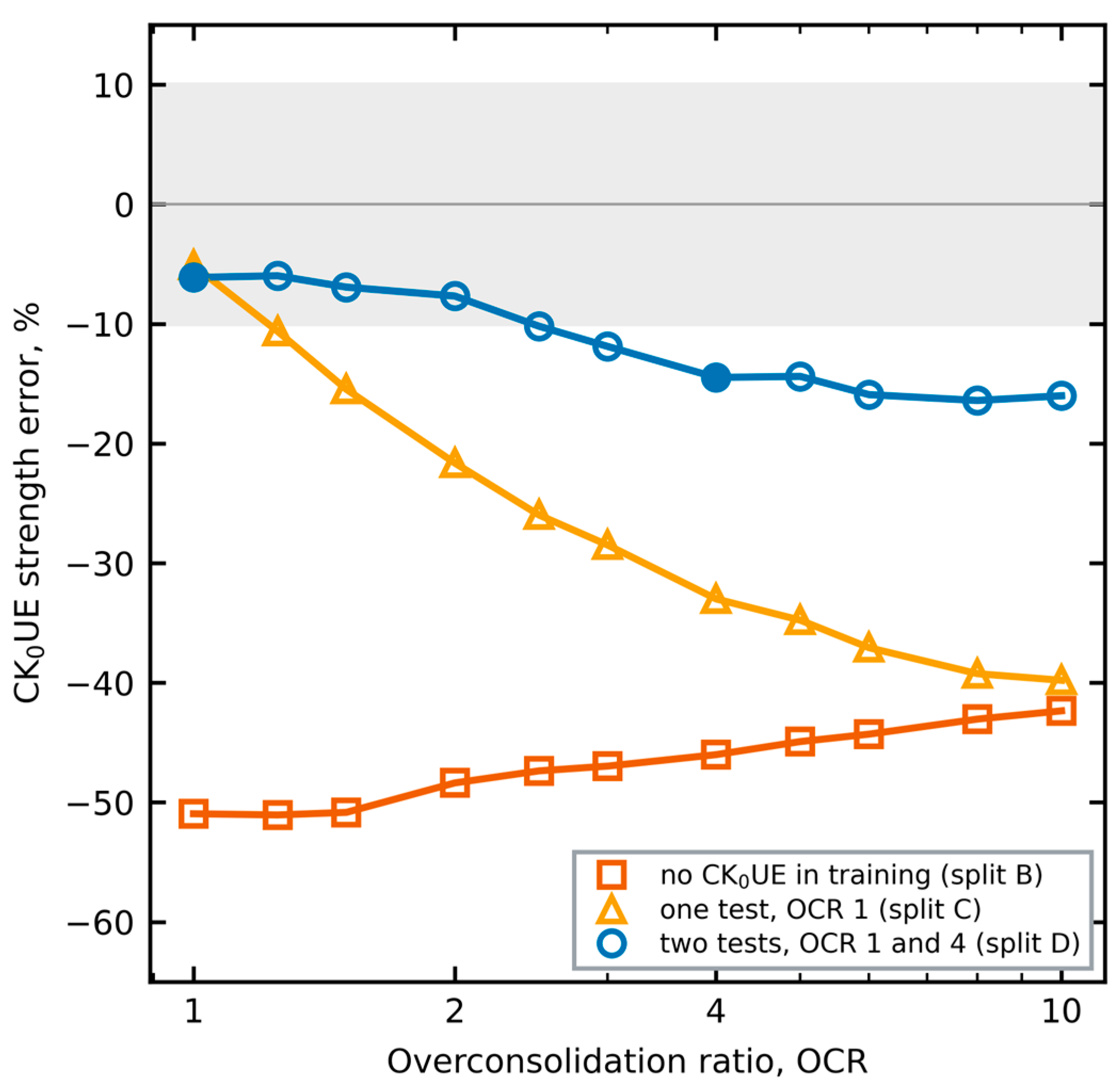
Figure 7.
Split B: CK0UE paths at σ′p = 4 pa predicted by a student that never saw extension of K0-consolidated clay. Open translucent markers: MIT-S1, thirteen points spaced evenly along each path; solid lines: student. Colours and marker shapes identify OCR = 1, 2, 4 and 8. Dotted grey line: critical stress ratio in extension.
Figure 7.
Split B: CK0UE paths at σ′p = 4 pa predicted by a student that never saw extension of K0-consolidated clay. Open translucent markers: MIT-S1, thirteen points spaced evenly along each path; solid lines: student. Colours and marker shapes identify OCR = 1, 2, 4 and 8. Dotted grey line: critical stress ratio in extension.
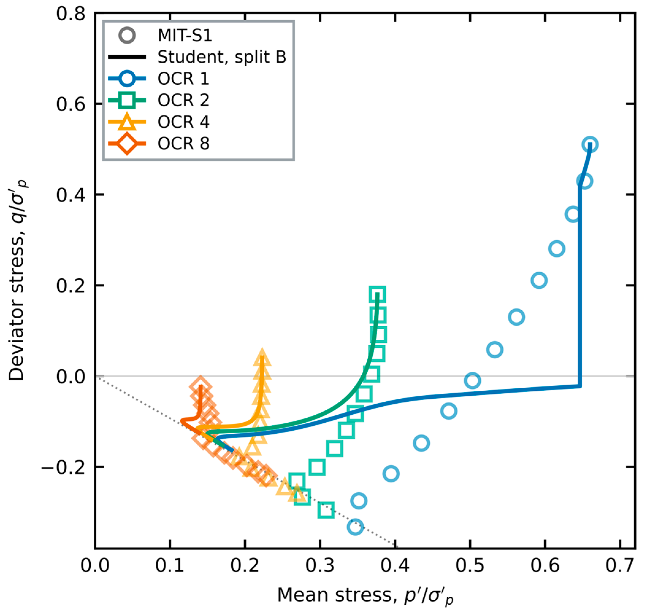
We attribute this to the structure of the model. In compression of K0 clay, the fabric and the stress ratio point the same way, and the potential, the fabric terms and the hardening exponent are exercised together. In extension the stress ratio reverses while the initial fabric does not, so the response depends on the extension branch of the potential and on how the fabric rotates towards extension, and neither appears in compression data. Isotropic extension does not fill the gap, because its fabric starts isotropic: split B contains every CIUE path and still fails on CK0UE.
3.5. The Extracted Potential and Its Uniqueness
Figure 8 shows the dilatancy of the final potential. With isotropic fabric, the zero-dilatancy ratio in compression falls as R decreases, so overconsolidated states start to dilate at a lower stress ratio. With K0 fabric, the compression branches move closer together and become steeper. The potential is a well-defined, differentiable function within the domain stated in Section 2.5.3. The constants that produce it, however, are not unique (Table 5).
Three observations show this. First, runs of the same configuration from different seeds reach validation losses within about 20% of each other, with different constants. Second, the potential constants changed markedly as the hardening exponent and the kinematic shift were learned (AC0 = 1.61 at S6, 1.29 at S7 and 1.23 at S8): part of what the potential had absorbed at S6 was a hardening error. Third, splits A and B give different calibrations of similar accuracy on the shared paths (Table 5). The problem is multimodal. What has been extracted is a functional form with one admissible calibration, not a unique parameter set [60].
For a user, the non-uniqueness has two consequences. First, the constants in Table 5 are not material properties of BBC: they are one admissible set for the extracted form, and another seed would return a different set with nearly the same predictions. Second, transfer to a new clay should keep the form and re-calibrate only the constants that a standard test controls, as done with Ψ and Ω in Section 3.10, rather than reuse every constant. What transfers is the functional form; how far its constants can be fixed by fewer, better chosen tests is a question for a calibration study. The non-uniqueness is also a property of the data. Undrained triaxial paths constrain combinations of constants rather than each constant, because a path depends on the balance between plastic and elastic stiffness and on the direction of flow, and several combinations of Ψ, Ω, the hardening exponent and the potential give nearly the same path. Drained paths and oedometer unloading would separate some of these combinations; they were not used here (Section 4.3).
3.6. Peak and Post-Peak Softening
MIT-S1 predicts a peak followed by softening in undrained compression of normally consolidated K0 clay: the deviator at the end of the path is 23% below the peak at σ′p = 4 pa (peak-to-end ratio 1.300) and 21% below at 8 pa (1.267). The final model places the peak at the right strain but softens much less (ratio 1.069 at both stresses), because the validation loss rewards the end of the path only weakly. The plastic modulus has one term that controls this, Mk − ξ⟨α⟩R8 for η > 0, which lowers the bounding modulus near the normally consolidated state of K0 fabric only. With ξ = 1.5 and all other constants re-fitted, the ratio becomes 1.331 at 4 pa and 1.302 at the held-out 8 pa (Figure 9), with a validation loss 6% above the final model and 88% (isotropic) and 94% (K0) of test paths still within 10% in strength. When ξ was left free from this start, the optimizer returned values of 0.12–1.15 at higher validation loss. Softening is therefore available in the extracted model, as in the base teardrop model [20], but it is not selected by a loss that weights the whole path. The choice between the two is a choice of purpose: the final model for strength and the whole stress path, the softening variant where the post-peak response of normally consolidated K0 clay matters.
3.7. Reduction to the Reference Potential
A constrained variant enforces g = g₀ at α = 0. The reference AJOP-T potential is then recovered exactly for isotropic fabric, and all corrections act through the fabric. With the same protocol up to stage S4, it keeps the path accuracy: NRMSE is below 10% for 94% of paths in both groups. The strength accuracy of K0 paths, however, falls from 81% to 44% of paths passing (Table 4, S4-O). The reference potential is too dilative for this teacher. Corrections that act only through the fabric cannot fully compensate.
3.8. Second Teacher
Table 6 compares the students on Lower Cromer Till. With the reference model (a), every path passes the NRMSE criterion, but only 38% of isotropic and 25% of K0 paths are within 10% in strength. With the BBC potential and hardening frozen (b), the mean strength error falls from 16.9% to 7.5% for isotropic and from 19.9% to 8.6% for K0 paths. Re-fitting everything (c) gives no further gain at this budget; row (a) used a smaller budget (one seed, 1400 evaluations), so part of the difference may reflect the unequal optimization budgets. The weak mode is again extension of K0 clay, which is under-predicted on every test path.

Table 6.
Transfer to a second teacher, Lower Cromer Till: test performance of students fitted on the training paths. Mean NRMSE and mean |su error| over the test sets; pass rate in parentheses.
Table 6.
Transfer to a second teacher, Lower Cromer Till: test performance of students fitted on the training paths. Mean NRMSE and mean |su error| over the test sets; pass rate in parentheses.
| Student | CIU NRMSE | CIU |su| error | CK0U NRMSE | CK0U |su| error |
| (a) reference AJOP-T, constants re-fitted | 0.058 (100%) | 16.9% (38%) | 0.041 (100%) | 19.9% (25%) |
| (b) BBC potential and hardening frozen | 0.032 (100%) | 7.5% (69%) | 0.031 (100%) | 8.6% (56%) |
| (c) all constants re-fitted | 0.032 (100%) | 7.4% (75%) | 0.029 (100%) | 9.7% (50%) |
16 isotropic and 16 K0 test paths. Pass rates: NRMSE < 10% and |su error| < 10%, counted separately. Rows (b) and (c): S8 model, 2000 evaluations, two seeds, lowest validation loss; row (a): 1400 evaluations, one seed.
3.9. Laboratory Strength
Figure 10 compares undrained strengths with laboratory data. For BBC in CK0UC, the teacher is within 5% of the data of Sheahan (Figure 10a). The data of Fayad are higher at OCR ≥ 2, and the teacher follows Sheahan. For LCT, the teacher under-predicts CK0UC by only 0–7%, but CIUC by 15–32% and CIUE by 9–28%, increasingly with OCR (Figure 10b). The source reports the same under-prediction for isotropically consolidated LCT [8]. The student inherits these biases. On BBC CK0UC, the final student is within 5% of the teacher at every OCR and within 10% of the data of Sheahan; the OCR trend of stage S6 (+21% to −19% against the teacher) is gone. Against the LCT data its error ranges over −11% to +1% (CK0UC), −36% to −10% (CIUC) and −18% to −3% (CIUE). A student that imitates its teacher where the teacher is biased inherits the bias; the LCT isotropic data show where this matters, and Section 3.11 shows how it can be avoided.
3.10. Five Clays with Published Parameters
Table 7 and Figure 11 and Figure 12 give the results for five clays calibrated from one test each, with the reference AJOP-T and with the model extracted from BBC. London Clay (data of Gasparre, as compiled in [20]; λ, κ, M and e₀ from the same source) is added to the four clays of Section 2.7 with the same protocol: Ψ and Ω are calibrated on the test at OCR = 1, and the tests at OCR = 2, 6 and 18.7 are predicted. The peak strength is compared within the measured range of each test, because a model path that continues beyond the last measured point is not a prediction of a measured quantity. The extracted model lowers the mean stress path error for kaolin and Eastern Osaka clay, and raises it for Fujinomori clay, Bangkok clay and London Clay.
Per clay, the mean ESP-RMSE changes from Fujinomori clay 0.051 to 0.063; kaolin 0.042 to 0.025; Eastern Osaka clay 0.096 to 0.088; Bangkok clay 0.050 to 0.051; London Clay 0.018 to 0.029 (reference to extracted). For Fujinomori clay the whole increase comes from the extension test: after the deviator stress reaches about −0.5 p′ref, the extracted model turns towards larger mean stress, whereas the measured path continues at nearly constant p′ (Figure 11a). Eastern Osaka clay remains a stress test: both models under-predict the strength of its overconsolidated tests, which points to the structure of this natural clay [70]. For Bangkok clay, the measured paths end at a stress ratio of about 0.76, below the critical ratio M = 0.90 used here, and the strains include creep; neither effect is in either model. London Clay has the largest κ/λ of the five clays (0.38) and the highest OCR (18.7), far beyond the training range of the teacher (OCR ≤ 8); there the extracted model over-predicts the strength of the tests at OCR = 6 and 18.7 by +34% and +21%, against +10% and +7% for the reference.
The picture is mixed. Where strains were reported, the extracted model lowers the q–ε error for Fujinomori clay (0.124 to 0.045) and kaolin (0.060 to 0.033) and raises it for Bangkok clay (0.071 to 0.088); it lowers the mean strength error for Fujinomori clay and Eastern Osaka clay, and its stress path error is higher for Fujinomori clay, Bangkok clay and London Clay. With the extracted potential and the reference hardening exponent, the mean ESP-RMSE is Fujinomori clay 0.064; kaolin 0.028; Eastern Osaka clay 0.093; Bangkok clay 0.051; London Clay 0.024, so neither component alone accounts for the differences. The model was extracted from one teacher, with one κ/λ and OCR ≤ 8, and never saw these data. The evidence supports it as an alternative default to be checked against one or two tests of the clay at hand, not as a calibrated law for any clay.
Comparing the three variants separates the two learned components. For kaolin, the extracted potential alone lowers the stress path error from 0.042 to 0.028, and the learned hardening exponent adds a smaller gain (0.025); the improvement is mainly a matter of flow direction. For Fujinomori clay the error is almost the same with and without the learned hardening (0.064 and 0.063), so the extension response described above comes from the potential. For London Clay both components add to the error: 0.018 for the reference, 0.024 with the extracted potential and 0.029 with both. This agrees with where the errors occur: the learned hardening raises the strength at high OCR, and the London tests lie far outside the OCR range of the teacher.
For a user, this suggests a simple procedure. For a clay whose κ/λ and OCR range are close to those of the teacher, the extracted model can serve as a default after Ψ and Ω are calibrated on one normally consolidated test. Where κ/λ is much larger or the OCR much higher, as for London Clay, the extracted potential with the reference hardening exponent was closer to the data. In either case a second test, preferably an overconsolidated or an extension test, should be predicted before the model is used.
The two clays that neither model predicts well mark the limits of what this teacher can pass on. Eastern Osaka clay is a natural clay whose overconsolidated strength depends partly on structure, and MIT-S1 has no mechanism for structure or its destruction, so no student of MIT-S1 can learn it. Weathered Bangkok Clay creeps during shearing, and its measured paths stop below the critical ratio used here. Both gaps call for a different teacher, or one extended with structure and rate effects, rather than more data from the present one.
3.11. Training Only Where the Teacher Is Accurate
Figure 13 compares the isotropic strengths of LCT. The teacher under-predicts the laboratory values at every OCR, by a mean of 20% over the ten measurements. The student of split K with all constants re-fitted, selected by validation loss, has a mean error of 12% (CIUC 19%, CIUE 5%); the other seed gives 9%. It never saw an isotropic path, so this is a prediction from the K0 paths and the structure of the model, and it is closer to the laboratory than its teacher. The gain is not uniform: the selected run over-predicts CIUC at OCR = 10 by +38%. With the BBC potential and hardening frozen, the student follows the teacher’s bias (mean error 24%). The evidence rests on ten measurements of one clay; it shows that a student can correct a teacher where the teacher is known to be wrong, not that it always will.
3.12. Many Synthetic Clays from One Generator
Table 8 gives the whole-curve errors. Relative to the single-teacher model, round 1 of the generator raised the stress path error of no clay and lowered it by at most 0.006. These changes are small. Its stress–strain error was the same for kaolin, slightly lower for Fujinomori clay (0.044 against 0.045) and higher for Weathered Bangkok Clay (0.106 against 0.088). Against the reference AJOP-T, its stress path error is lower for three of the five clays (kaolin, Eastern Osaka clay, Weathered Bangkok Clay) and higher for Fujinomori clay and London Clay. For London Clay the learned hardening still over-predicts strength at OCR = 6 (mean strength error 23%, against 12% for the reference). On the BBC test paths it keeps NRMSE below 10% for every path, with strength within 10% for 94% of isotropic and 81% of K0 paths, against 94% and 100% for the single-teacher model.
Round 2 tested whether more and wider training data would help. With eight more clays and OCR up to 16, the stress path error was at or below the reference for two of the five clays, London Clay did not improve (strength error 24%), and on BBC the K0 strength was within 10% for only 69% of test paths. Its BBC validation loss was also higher (0.00153 against 0.00137 for round 1), so the selection rule fixed before the runs keeps round 1. That more clays and a wider OCR range did not reduce the error suggests a limitation of the hardening form. The optimization budget, the distribution of the synthetic clays and the alternating scheme are alternative explanations that this study did not separate.
Table 8 also shows what the generator does not change. The order of the clays from best to worst predicted is the same for the single-teacher model and round 1, and nearly the same for round 2. The errors are set mainly by the clay, its structure, creep and stress history relative to the range of the teacher, rather than by which teacher data the student saw. This is expected when the form of the model is fixed and only its constants move: more varied data may help only a form that is flexible enough to use them.
4. Discussion
4.1. What Was Extracted
The extraction returns two forms: a kinematic Nova-type stress–dilatancy relation [6,62] with a fabric-dependent slope and zero-dilatancy ratio, written as a smooth plastic potential inside a bounding-surface model [15,23], and a closed-form exponent of the bounding plastic modulus. Together they reproduce every held-out undrained path of both consolidation types within the NRMSE criterion, including the OCR and stress-level extrapolations, and match the teacher’s flow direction with a mean mismatch of 7.8° (largest 21°, on one extrapolated CK0UE path). The forms were chosen from training labels and selection used validation loss only, although intermediate test results guided which mechanism was added next (Section 2.3). Unlike a black-box surrogate [33,36,47], the result can be read, implemented and checked like any other flow and hardening rule [24,72]. Two lessons are general. A potential learned with a wrong hardening law absorbs part of the hardening error (Section 3.5), so the two must be learned together. And more teacher data helps only where it covers the loading mode: 56 more compression and extension paths raised the strength pass rate, while the tested training sets without CK0UE paths did not identify its extension response (Section 3.4).
The teacher need not be treated as ground truth. Used as a data source, it can be restricted to where it agrees with laboratory data (Section 3.11) or sampled over many parameter sets (Section 3.12). The first design moved the student closer to laboratory data than its teacher. The second changed the laboratory errors only slightly, in both directions, and adding clays did not help. Restricting the teacher to where it is accurate is therefore the design we recommend; the generator design may need a more flexible hardening law before more data can pay off.
The constants should not be read as material properties. Two splits give different calibrations of equal quality, and some constants move to the edge of their range. This is a known risk when a model with many interacting parameters is fitted to a limited set of paths [37,60,69]. Adding drained or oedometric paths, which constrain κ and ν separately [12,19], is the clearest next step.
4.2. Why the Neural Route Failed and the Closed Form Worked
Two features of the problem favour a low-dimensional closed form. First, the loss along a full path is only piecewise smooth. Gradient training of a network with hundreds of weights stalls on such a loss [59], while an evolution strategy over about twenty-five constants copes with it [68]. Second, local flow labels are cheap to fit but do not fix the path. A small error in flow direction early on changes the state, and hence every later increment [30,31]. The labels were most useful as evidence for choosing the form [49,52].
Measuring flow consistency has a trap. One may compute the teacher’s plastic strains by subtracting the student’s elastic strains from the teacher’s total strains. The comparison then depends on the student’s own elastic constants. An optimiser can lower the apparent mismatch by changing elasticity rather than flow. In our trials, this circular measure reported 9° for a model whose mismatch against the teacher’s own plastic strains was about 22°. Recording the teacher’s own plastic strains removes the circularity at negligible cost. We recommend it for any distillation between constitutive models.
4.3. Limits
The model was extracted from undrained triaxial shear of one clay with one teacher. Its transfer was checked on a second teacher and on seven laboratory clays, but only for undrained paths and with the fabric switched off for the five clays without a fabric constant. Drained paths were not generated, because the lateral-stress control of the teacher’s driver did not converge at the elastic–plastic switch. Oedometer paths were generated but not used. Shearing starts from the measured stress after swelling, so the student does not predict K0 during swelling. This matters: the teacher’s swelling is purely hysteretic-elastic, whereas the student would need a stress-ratio-dependent elastic law or plastic strains on unloading to match it [9,16]. Strength in extension of K0 clay must be present in the training data. Finally, two teacher inputs (σ′p and e₀) are approximate. The teacher is therefore a consistent reference model, not a calibrated description of BBC [4]. The laboratory checks also show what the student cannot learn from this teacher: structure and its destruction (Eastern Osaka), creep (Bangkok), and any bias of the teacher itself (isotropic LCT). The hardening exponent learned from BBC added a small gain for kaolin and raised the error for London Clay; it should be re-checked for clays with a much larger κ/λ or a higher OCR than BBC.
5. Conclusions
A plastic potential and a hardening exponent for a compact bounding-surface model were learned from an advanced clay model and distilled to closed forms. The main findings are as follows:
- Recording the teacher’s own plastic strains, which leaves its stresses unchanged, gives an unbiased measure of flow consistency. Decomposing the teacher’s strains with the student’s elastic law does not;
- A neural potential trained end-to-end did not improve held-out predictions. An inverse dilatancy analysis instead identified a Nova-type stress–dilatancy form, consistent with the linear dilatancy measured on two clays, that becomes kinematic when measured from the fabric axis;
- A systematic OCR bias of undrained strength was traced to the fixed hardening exponent and removed by learning it as a closed form. Trained on 96 teacher paths, the final student reproduced all 32 held-out undrained paths with NRMSE below 10%, undrained strength within 10% for 94% of isotropic and 100% of K0 test paths, and a mean flow-direction mismatch of 7.8°;
- Peak and post-peak softening of normally consolidated K0 clay are reproduced by a constrained variant (peak-to-end ratio 1.30 on a held-out stress level, against 1.27 for the teacher);
- Extension of K0 clay was not learned from compression data in the tested configurations; two extension tests (OCR = 1 and 4) reduced the mean strength error on 17 unseen extension paths to 11%, with 7 of them within 10%;
- Used as a data source rather than as ground truth, the teacher can give a student that is closer to laboratory data than the teacher: trained only where MIT-S1 matches laboratory data, a student predicted unseen isotropic strengths of Lower Cromer Till with a mean error of 12% against 20% for the teacher. Trained on twelve synthetic clays instead, the student reproduced the laboratory clays about as well as the single-teacher student, and twenty clays did not help, which suggests, but does not prove, that the hardening law limits the transfer;
- Frozen and moved to other clays, the extracted model improved strength prediction on a second MIT-S1 clay. On five laboratory clays calibrated from one test each it improved the q–ε curves of two of the three clays with reported strains and the stress paths of two clays; it inherits the κ/λ and OCR range of its teacher. The fitted constants are not unique.
Supplementary Materials
The following supporting information can be downloaded at the website of this paper posted on Preprints.org, File S1: source code of the differentiable student model and fitting protocol, the generated teacher dataset with its pre-declared split, the synthetic-clay generator settings, the fitted models and the scripts that reproduce all tables and figures.
Author Contributions
Conceptualization, N.K. and T.C.; methodology, N.K. and T.C.; software, T.C.; validation, N.K., T.C., Phongsakorn W. and Phongsatorn W.; formal analysis, N.K.; investigation, T.C., Phongsakorn W. and Phongsatorn W.; resources, S.E.-a., A.K., Phongsakorn W. and Phongsatorn W.; data curation, T.C.; writing—original draft preparation, N.K., Phongsakorn W. and Phongsatorn W.; writing—review and editing, N.K., A.K., S.E.-a. and S.S.; visualization, S.S., A.K. and S.E.-a.; supervision, A.K. and S.E.-a.; project administration, N.K.; funding acquisition, N.K. All authors have read and agreed to the published version of the manuscript.
Funding
This research project was financially supported by Mahasarakham University.
Data Availability Statement
The data generated and analysed in this study (teacher trajectories, plastic strain labels, split declaration and fitted models) and the code of the student model and the fitting are provided in Supplementary File S1. The teacher model, MIT-S1, is described in [8,9]; its code is not part of this work and is not distributed. Further inquiries can be directed to the corresponding author.
Acknowledgments
The student model and the fitting were implemented with the open-source libraries JAX [65], Optax [73], NumPy [74], SciPy [75] and pycma [76], and the figures were prepared with Matplotlib [77]. Generative AI tools (Claude Opus 5.5, Anthropic; ChatGPT, GPT-6.1 Sol Ultra, OpenAI) were used for language editing and to help prepare simulation, optimisation, data-processing and plotting scripts. The authors designed the study, formulated the constitutive model, selected the data and the checks reported, interpreted the results, and reviewed all AI-assisted material and outputs, which are provided in Supplementary File S1. The authors take full responsibility for this publication.
Conflicts of Interest
The authors declare no conflicts of interest.
References
- Ladd, C.C.; Foott, R. New design procedure for stability of soft clays. J. Geotech. Eng. Div. 1974, 100, 763–786. [Google Scholar] [CrossRef]
- Chotetanorm, C.; Kaewhanam, N.; Chatwong, T.; Inthidech, S.; Kampala, A.; Eua-apiwatch, S.; Sultornsanee, S. When is a constant compression index sufficient for pile downdrag? Joint drag and settlement criteria with laboratory and field checks. Buildings, submitted, 2026. [Google Scholar]
- Kaewhanam, N.; Chatwong, T.; Kampala, A.; Eua-apiwatch, S.; Sultornsanee, S. Evaluating compressibility assumptions for geological CO2 storage using linear and nonlinear compression evidence. Energies, submitted, 2026. [Google Scholar]
- Whittle, A.J.; DeGroot, D.J.; Ladd, C.C.; Seah, T.-H. Model prediction of anisotropic behavior of Boston Blue Clay. J. Geotech. Eng. 1994, 120, 199–224. [Google Scholar] [CrossRef]
- Wheeler, S.J.; Näätänen, A.; Karstunen, M.; Lojander, M. An anisotropic elastoplastic model for soft clays. Can. Geotech. J. 2003, 40, 403–418. [Google Scholar] [CrossRef]
- Dafalias, Y.F.; Manzari, M.T.; Papadimitriou, A.G. SANICLAY: Simple anisotropic clay plasticity model. Int. J. Numer. Anal. Methods Geomech. 2006, 30, 1231–1257. [Google Scholar] [CrossRef]
- Whittle, A.J.; Kavvadas, M.J. Formulation of MIT-E3 constitutive model for overconsolidated clays. J. Geotech. Eng. 1994, 120, 173–198. [Google Scholar] [CrossRef]
- Pestana-Nascimento, J.M. A Unified Constitutive Model for Clays and Sands. Sc.D. Thesis, Massachusetts Institute of Technology, Cambridge, MA, USA, 1994. [Google Scholar]
- Pestana, J.M.; Whittle, A.J. Formulation of a unified constitutive model for clays and sands. Int. J. Numer. Anal. Methods Geomech. 1999, 23, 1215–1243. [Google Scholar] [CrossRef]
- Roscoe, K.H.; Burland, J.B. On the generalised stress–strain behaviour of ‘wet’ clay. In Engineering Plasticity; Heyman, J., Leckie, F.A., Eds.; Cambridge University Press: London, UK, 1968; pp. 535–609. [Google Scholar]
- Schofield, A.N.; Wroth, C.P. Critical State Soil Mechanics; McGraw-Hill: London, UK, 1968. [Google Scholar]
- Pestana, J.M.; Whittle, A.J. Compression model for cohesionless soils. Géotechnique 1995, 45, 611–631. [Google Scholar] [CrossRef]
- Sloan, S.W. Substepping schemes for the numerical integration of elastoplastic stress–strain relations. Int. J. Numer. Methods Eng. 1987, 24, 893–911. [Google Scholar] [CrossRef]
- Kaewhanam, N.; Chatwong, T.; Sangiamsak, N.; Ladbut, N.; Chaiduangsri, N.; Inthidech, S.; Kampala, A.; Eua-apiwatch, S.; Sultornsanee, S. Safeguarded yield surface intersection under finite precision and discontinuous stress transformations; Mathematics, 2026. [Google Scholar]
- Dafalias, Y.F. Bounding surface plasticity. I: Mathematical foundation and hypoplasticity. J. Eng. Mech. 1986, 112, 966–987. [Google Scholar] [CrossRef]
- Dafalias, Y.F.; Herrmann, L.R. Bounding surface plasticity. II: Application to isotropic cohesive soils. J. Eng. Mech. 1986, 112, 1263–1291. [Google Scholar] [CrossRef]
- Hashiguchi, K. Subloading surface model in unconventional plasticity. Int. J. Solids Struct. 1989, 25, 917–945. [Google Scholar] [CrossRef]
- Kaewhanam, N.; Chaimoon, K. A simplified silty sand model. Appl. Sci. 2023, 13, 8241. [Google Scholar] [CrossRef]
- Phonchamni, N.; Chatwong, T.; Udomchai, A.; Sultornsanee, S.; Angkawisittpan, N.; Sangiamsak, N.; Kaewhanam, N. Refined consolidation settlement calculation based on the oedometer tests for normally and overconsolidated clays. Appl. Sci. 2025, 15, 5777. [Google Scholar] [CrossRef]
- Chatwong, T.; Kaewhanam, N.; Kaewplang, S.; Phonchamni, N.; Inthidech, S.; Kampala, A.; Sultornsanee, S. A robust constitutive model for clays over a wide range of plasticity and overconsolidation ratio (OCR) with symmetric, continuous curvature control of a teardrop yield surface. Symmetry 2026, 18, 215. [Google Scholar] [CrossRef]
- Matsuoka, H.; Nakai, T. Stress-deformation and strength characteristics of soil under three different principal stresses. Proc. Jpn. Soc. Civ. Eng. 1974, 232, 59–70. [Google Scholar] [CrossRef]
- Matsuoka, H.; Yao, Y.-P.; Sun, D. The Cam-clay models revised by the SMP criterion. Soils Found. 1999, 39, 81–95. [Google Scholar] [CrossRef]
- Chatwong, T.; Kaewhanam, N.; Kampala, A.; Eua-apiwatch, S.; Sultornsanee, S. AJOP-T: A high-order hardening law for continuous teardrop bounding surface plasticity. Mathematics 2026, 14, 2975. [Google Scholar] [CrossRef]
- Kaewhanam, N.; Chatwong, T.; Kampala, A.; Eua-apiwatch, S.; Sultornsanee, S. Continuous geometry, continuous flow, continuous compression: A numerical component-interaction assessment for fractional clay plasticity. Fractal Fract. 2026, 10, 501. [Google Scholar] [CrossRef]
- Kaewhanam, N.; Chatwong, T.; Kampala, A.; Eua-apiwatch, S.; Sultornsanee, S. Closed-form critical-state Caputo flow for a teardrop bounding surface: Operator semantics and factorial consequences. Fractal Fract. 2026, 10, 585. [Google Scholar] [CrossRef]
- Kaewhanam, N.; Chatwong, T.; Kampala, A.; Eua-apiwatch, S.; Sultornsanee, S. Terminal compatibility and admissibility of a meridional Caputo flow rule in transformed-stress clay plasticity. Fractal Fract. 2026, 10, 704. [Google Scholar] [CrossRef]
- Sangiamsak, N.; Kaewhanam, N.; Chatwong, T.; Inthidech, S.; Kampala, A.; Eua-apiwatch, S.; Sultornsanee, S. Compatibility-constrained fractional AJOP-T bounding-surface plasticity: Work conjugacy, complete consistency and plastic power. Fractal Fract, submitted, 2026. [Google Scholar]
- Ghaboussi, J.; Garrett, J.H.; Wu, X. Knowledge-based modeling of material behavior with neural networks. J. Eng. Mech. 1991, 117, 132–153. [Google Scholar] [CrossRef]
- Lefik, M.; Schrefler, B.A. Artificial neural network as an incremental non-linear constitutive model for a finite element code. Comput. Methods Appl. Mech. Eng. 2003, 192, 3265–3283. [Google Scholar] [CrossRef]
- Mozaffar, M.; Bostanabad, R.; Chen, W.; Ehmann, K.; Cao, J.; Bessa, M.A. Deep learning predicts path-dependent plasticity. Proc. Natl. Acad. Sci. USA 2019, 116, 26414–26420. [Google Scholar] [CrossRef]
- Bonatti, C.; Mohr, D. On the importance of self-consistency in recurrent neural network models representing elasto-plastic solids. J. Mech. Phys. Solids 2022, 158, 104697. [Google Scholar] [CrossRef]
- Kirchdoerfer, T.; Ortiz, M. Data-driven computational mechanics. Comput. Methods Appl. Mech. Eng. 2016, 304, 81–101. [Google Scholar] [CrossRef]
- Zhang, P.; Yin, Z.-Y.; Jin, Y.-F. State-of-the-art review of machine learning applications in constitutive modeling of soils. Arch. Comput. Methods Eng. 2021, 28, 3661–3686. [Google Scholar] [CrossRef]
- Rezazadeh Eidgahee, D.; Shiri, H. Machine learning–enhanced modeling of stress–strain behavior of frozen sandy soil. Geotechnics 2024, 4, 1228–1245. [Google Scholar] [CrossRef]
- Lu, Y.; Mei, G. A deep learning approach for predicting two-dimensional soil consolidation using physics-informed neural networks (PINN). Mathematics 2022, 10, 2949. [Google Scholar] [CrossRef]
- Mitelman, A.; Yang, B.; Elmo, D. Implementation of surrogate models for the analysis of slope problems. Geosciences 2023, 13, 99. [Google Scholar] [CrossRef]
- Lourenço, R.; Andrade-Campos, A.; Georgieva, P. The use of machine-learning techniques in material constitutive modelling for metal forming processes. Metals 2022, 12, 427. [Google Scholar] [CrossRef]
- Vilone, G.; Longo, L. Classification of explainable artificial intelligence methods through their output formats. Mach. Learn. Knowl. Extr. 2021, 3, 615–661. [Google Scholar] [CrossRef]
- Masi, F.; Stefanou, I.; Vannucci, P.; Maffi-Berthier, V. Thermodynamics-based artificial neural networks for constitutive modeling. J. Mech. Phys. Solids 2021, 147, 104277. [Google Scholar] [CrossRef]
- González, D.; García-González, A.; Chinesta, F.; Cueto, E. A data-driven learning method for constitutive modeling: Application to vascular hyperelastic soft tissues. Materials 2020, 13, 2319. [Google Scholar] [CrossRef]
- Vlassis, N.N.; Sun, W. Sobolev training of thermodynamic-informed neural networks for interpretable elasto-plasticity models with level set hardening. Comput. Methods Appl. Mech. Eng. 2021, 377, 113695. [Google Scholar] [CrossRef]
- Shang, H.; Niu, L.; Tian, Z.; Fan, C.; Zhang, Z.; Lou, Y. Multi-scale anisotropic yield function based on neural network model. Materials 2025, 18, 714. [Google Scholar] [CrossRef]
- Mouratidou, A.D.; Stavroulakis, G.E. A neural network constitutive model and automatic stiffness evaluation for multiscale finite elements. Appl. Sci. 2025, 15, 3697. [Google Scholar] [CrossRef]
- Linka, K.; Hillgärtner, M.; Abdolazizi, K.P.; Aydin, R.C.; Itskov, M.; Cyron, C.J. Constitutive artificial neural networks: A fast and general approach to predictive data-driven constitutive modeling by deep learning. J. Comput. Phys. 2021, 429, 110010. [Google Scholar] [CrossRef]
- Raissi, M.; Perdikaris, P.; Karniadakis, G.E. Physics-informed neural networks: A deep learning framework for solving forward and inverse problems involving nonlinear partial differential equations. J. Comput. Phys. 2019, 378, 686–707. [Google Scholar] [CrossRef]
- Zhou, M.; Mei, G.; Xu, N. Enhancing computational accuracy in surrogate modeling for elastic–plastic problems by coupling S-FEM and physics-informed deep learning. Mathematics 2023, 11. [Google Scholar] [CrossRef]
- Zhang, G.; Xu, T.; Xu, J.; Wang, H. A graph-structured, physics-informed DeepONet neural network for complex structural analysis. Mach. Learn. Knowl. Extr. 2025, 7, 137. [Google Scholar] [CrossRef]
- Jurj, S.L. Physics structure-informed neural networks in the TinyML pipeline: Antisymmetry preservation, deployment accounting, and training-budget sensitivity. Mach. Learn. Knowl. Extr. 2026, 8, 267. [Google Scholar] [CrossRef]
- Schmidt, M.; Lipson, H. Distilling free-form natural laws from experimental data. Science 2009, 324, 81–85. [Google Scholar] [CrossRef]
- Brunton, S.L.; Proctor, J.L.; Kutz, J.N. Discovering governing equations from data by sparse identification of nonlinear dynamical systems. Proc. Natl. Acad. Sci. USA 2016, 113, 3932–3937. [Google Scholar] [CrossRef]
- Flaschel, M.; Kumar, S.; De Lorenzis, L. Unsupervised discovery of interpretable hyperelastic constitutive laws. Comput. Methods Appl. Mech. Eng. 2021, 381, 113852. [Google Scholar] [CrossRef]
- Cranmer, M.; Sanchez-Gonzalez, A.; Battaglia, P.; Xu, R.; Cranmer, K.; Spergel, D.; Ho, S. Discovering symbolic models from deep learning with inductive biases. Adv. Neural Inf. Process. Syst. 2020, 33, 17429–17442. [Google Scholar]
- Hinton, G.; Vinyals, O.; Dean, J. Distilling the knowledge in a neural network. arXiv 2015, arXiv:1503.02531. [Google Scholar] [CrossRef]
- Buciluă, C.; Caruana, R.; Niculescu-Mizil, A. Model compression. In Proceedings of the 12th ACM SIGKDD International Conference on Knowledge Discovery and Data Mining, Philadelphia, PA, USA, 20–23 August 2006; pp. 535–541. [Google Scholar] [CrossRef]
- Krčmar, T.; Šabanović, D.; Švarcmajer, M.; Lukić, I. What knowledge transfers in tabular anomaly detection? A teacher–student distillation analysis. Mach. Learn. Knowl. Extr. 2026, 8, 60. [Google Scholar] [CrossRef]
- Limhengha, S.; Sudsawat, S. Explainable surrogate-based knowledge extraction from DEM simulations: Cross-system algorithm selection and SHAP interpretability for granular material handling optimization. Mach. Learn. Knowl. Extr. 2026, 8, 229. [Google Scholar] [CrossRef]
- Rabbi, M.F. Optimizing carbon capture efficiency: Knowledge extraction from process simulations of post-combustion amine scrubbing. Mach. Learn. Knowl. Extr. 2026, 8, 87. [Google Scholar] [CrossRef]
- Barletta, G.; Trezza, G.; Chiavazzo, E. Learning effective good variables from physical data. Mach. Learn. Knowl. Extr. 2024, 6, 1597–1618. [Google Scholar] [CrossRef]
- Kenzhebek, Y.; Imankulov, T.; Bekele, S.D.; Mukhambetzhanov, S. Physics-informed neural networks for coupled non-isothermal two-phase flow in porous media: Training pathologies, remedies, and the role of gradient conflict. Mach. Learn. Knowl. Extr. 2026, 8, 266. [Google Scholar] [CrossRef]
- Ladbut, N.; Kaewhanam, N.; Chatwong, T.; Inthidech, S.; Kampala, A.; Eua-apiwatch, S.; Sultornsanee, S. Benchmarking fractional and Prony memory in viscoplasticity with directional hardening. Fractal Fract, submitted, 2026. [Google Scholar]
- Rowe, P.W. The stress-dilatancy relation for static equilibrium of an assembly of particles in contact. Proc. R. Soc. Lond. A 1962, 269, 500–527. [Google Scholar] [CrossRef]
- Nova, R.; Wood, D.M. A constitutive model for sand in triaxial compression. Int. J. Numer. Anal. Methods Geomech. 1979, 3, 255–278. [Google Scholar] [CrossRef]
- Lashkari, A. Recommendations for extension and re-calibration of an existing sand constitutive model taking into account varying non-plastic fines content. Soil Dyn. Earthq. Eng. 2014, 61–62, 212–238. [Google Scholar] [CrossRef]
- Xu, B.; Chen, K.; Pang, R. A bounding surface model for overconsolidated clays with unified plastic potential function in triaxial and general stress state. Comput. Geotech. 2024, 172, 106429. [Google Scholar] [CrossRef]
- Bradbury, J.; Frostig, R.; Hawkins, P.; Johnson, M.J.; Leary, C.; Maclaurin, D.; Necula, G.; Paszke, A.; VanderPlas, J.; Wanderman-Milne, S.; et al. JAX: Composable Transformations of Python+NumPy Programs, 2018. Available online: http://github.com/jax-ml/jax (accessed on 1 November 2026).
- Baydin, A.G.; Pearlmutter, B.A.; Radul, A.A.; Siskind, J.M. Automatic differentiation in machine learning: A survey. J. Mach. Learn. Res. 2018, 18, 1–43. [Google Scholar]
- Kingma, D.P.; Ba, J. Adam: A method for stochastic optimization. In Proceedings of the 3rd International Conference on Learning Representations (ICLR), 2015. [Google Scholar]
- Hansen, N.; Ostermeier, A. Completely derandomized self-adaptation in evolution strategies. Evol. Comput. 2001, 9, 159–195. [Google Scholar] [CrossRef]
- Zhang, Y.; Song, H.; Yang, Y. Intelligent calibration of the cycle liquefaction constitutive model parameter using a genetic algorithm-based optimization framework. Geosciences 2026, 16, 18. [Google Scholar] [CrossRef]
- Adachi, T.; Oka, F.; Hirata, T.; Hashimoto, T.; Nagaya, J.; Mimura, M.; Pradhan, T.B.S. Stress–strain behavior and yielding characteristics of Eastern Osaka clay. Soils Found. 1995, 35, 1–13. [Google Scholar] [CrossRef]
- Balasubramaniam, A.S.; Hwang, Z.-M. Yielding of weathered Bangkok clay. Soils Found. 1980, 20, 1–15. [Google Scholar] [CrossRef]
- Inthidech, S.; Kaewhanam, N.; Chatwong, T.; Kampala, A.; Eua-apiwatch, S.; Sultornsanee, S. Defining function dependence of Riemann–Liouville plastic flow on a common convex yield surface. Fractal Fract, 2026, submitted. [Google Scholar]
- DeepMind; Babuschkin, I.; Baumli, K.; Bell, A.; Bhupatiraju, S.; Bruce, J.; Buchlovsky, P.; Budden, D.; Cai, T.; Clark, A.; et al. The DeepMind JAX Ecosystem, 2020. Available online: http://github.com/google-deepmind (accessed on 2 November 2026).
- Harris, C.R.; Millman, K.J.; van der Walt, S.J.; Gommers, R.; Virtanen, P.; Cournapeau, D.; Wieser, E.; Taylor, J.; Berg, S.; Smith, N.J.; et al. Array programming with NumPy. Nature 2020, 585, 357–362. [Google Scholar] [CrossRef]
- Virtanen, P.; Gommers, R.; Oliphant, T.E.; Haberland, M.; Reddy, T.; Cournapeau, D.; Burovski, E.; Peterson, P.; Weckesser, W.; Bright, J.; et al. SciPy 1.0: Fundamental algorithms for scientific computing in Python. Nat. Methods 2020, 17, 261–272. [Google Scholar] [CrossRef]
- Hansen, N.; Akimoto, Y.; Baudis, P. CMA-ES/pycma on Github; Zenodo, 2019. [Google Scholar] [CrossRef]
- Hunter, J.D. Matplotlib: A 2D graphics environment. Comput. Sci. Eng. 2007, 9, 90–95. [Google Scholar] [CrossRef]
Figure 1.
Overview of the learning pipeline: the three uses of the teacher (left), the data (second column), the student and its fitting stages (third column), and the selection rule and the checks beyond the teacher (right). The small glyphs are schematic: sampled clays, the data split, the CMA-ES population contracting towards its mean, and the training and validation losses.
Figure 1.
Overview of the learning pipeline: the three uses of the teacher (left), the data (second column), the student and its fitting stages (third column), and the selection rule and the checks beyond the teacher (right). The small glyphs are schematic: sampled clays, the data split, the CMA-ES population contracting towards its mean, and the training and validation losses.
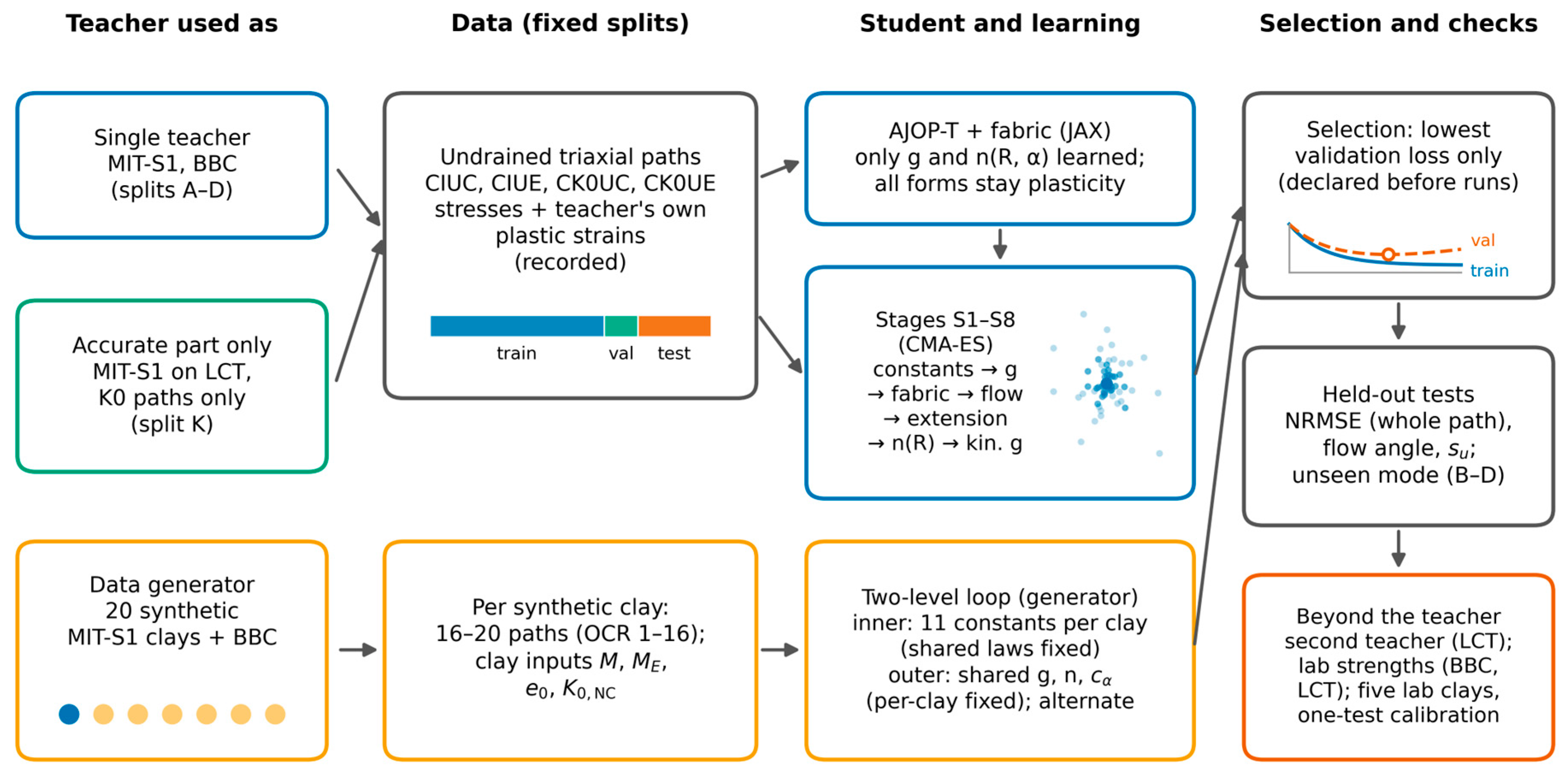
Figure 2.
Dilatancy d = dεvp/dεqp against the stress ratio η along three test paths at σ′p = 4 pa: MIT-S1, computed from its own plastic strain increments (black solid line); the student before learning, stage S1 (red dotted line); and the student with the learned potential, stage S8 (blue dashed line). (a) CIUC, OCR = 5; (b) CK0UC, OCR = 2.5; (c) CK0UE, OCR = 5.
Figure 2.
Dilatancy d = dεvp/dεqp against the stress ratio η along three test paths at σ′p = 4 pa: MIT-S1, computed from its own plastic strain increments (black solid line); the student before learning, stage S1 (red dotted line); and the student with the learned potential, stage S8 (blue dashed line). (a) CIUC, OCR = 5; (b) CK0UC, OCR = 2.5; (c) CK0UE, OCR = 5.
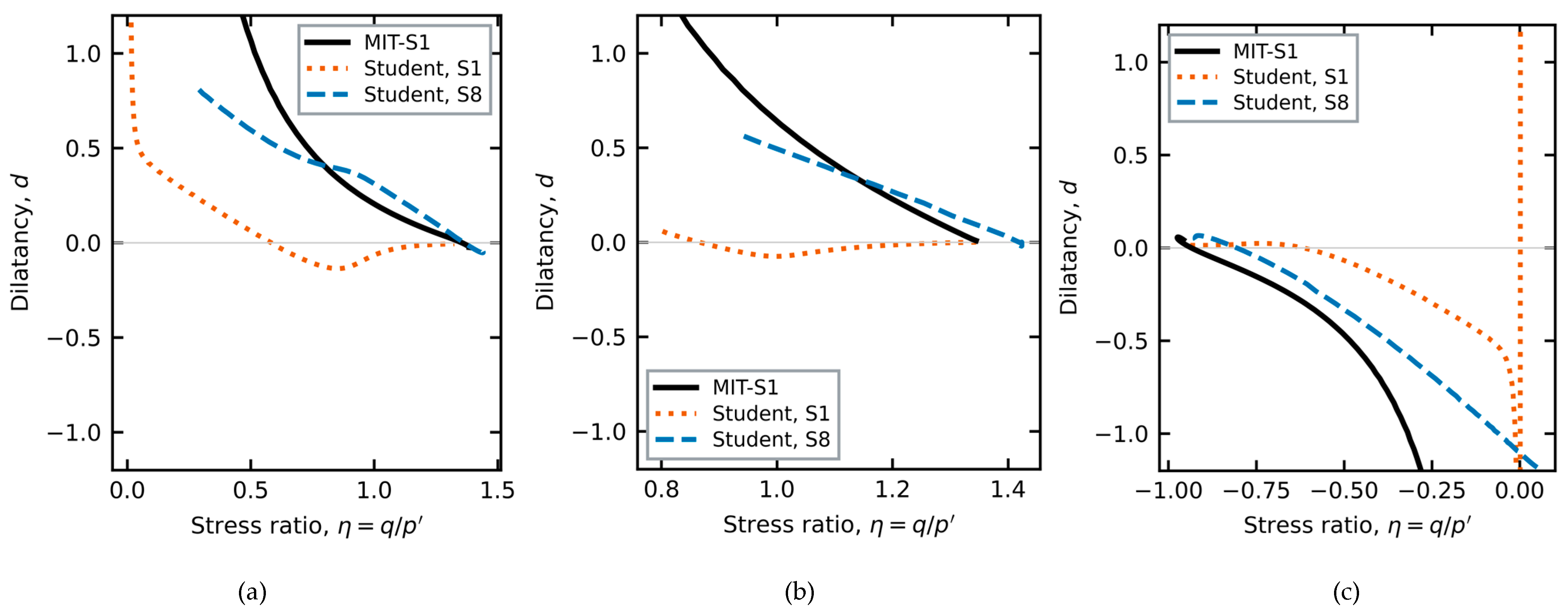
Figure 3.
Two-level training on many clays generated with MIT-S1. Inner level: the constants of each clay, with the shared laws fixed. Outer level: the shared laws (potential, hardening exponent and kinematic constant), with the per-clay constants fixed. BBC keeps its training, validation and test roles; the laboratory clays are used only for testing.
Figure 3.
Two-level training on many clays generated with MIT-S1. Inner level: the constants of each clay, with the shared laws fixed. Outer level: the shared laws (potential, hardening exponent and kinematic constant), with the per-clay constants fixed. BBC keeps its training, validation and test roles; the laboratory clays are used only for testing.
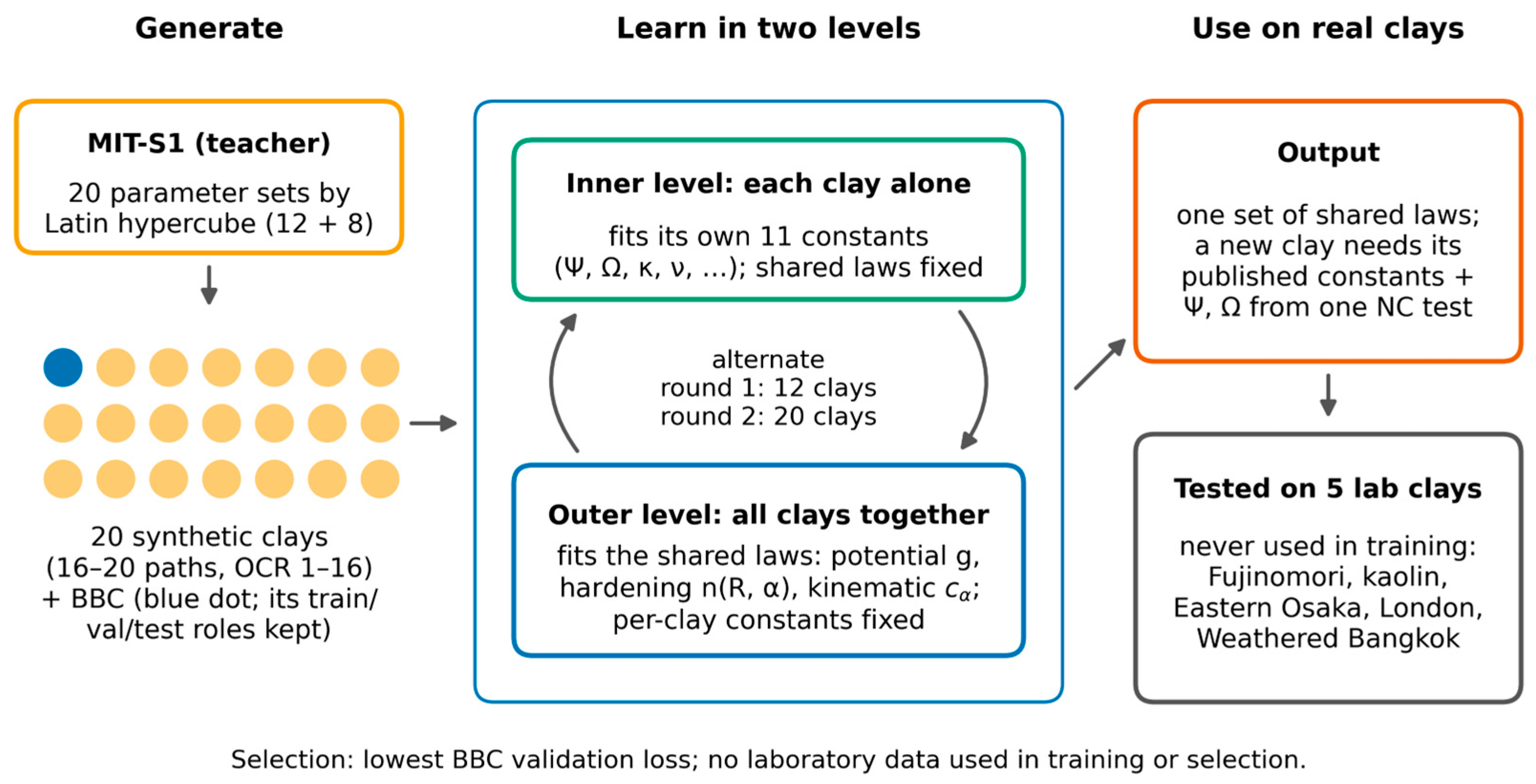
Figure 4.
Undrained effective stress paths of held-out trajectories at σ′p = 4 pa (none used in fitting or model selection). Open translucent markers: MIT-S1, thirteen points spaced evenly along each path; solid lines: student with the learned potential (stage S8). Colours and marker shapes identify OCR = 1.25, 2.5, 5 and 10; each OCR has a compression (q > 0) and an extension (q < 0) path. (a) Isotropic consolidation; (b) K0 consolidation. Dotted grey lines: critical stress ratios in compression and extension.
Figure 4.
Undrained effective stress paths of held-out trajectories at σ′p = 4 pa (none used in fitting or model selection). Open translucent markers: MIT-S1, thirteen points spaced evenly along each path; solid lines: student with the learned potential (stage S8). Colours and marker shapes identify OCR = 1.25, 2.5, 5 and 10; each OCR has a compression (q > 0) and an extension (q < 0) path. (a) Isotropic consolidation; (b) K0 consolidation. Dotted grey lines: critical stress ratios in compression and extension.
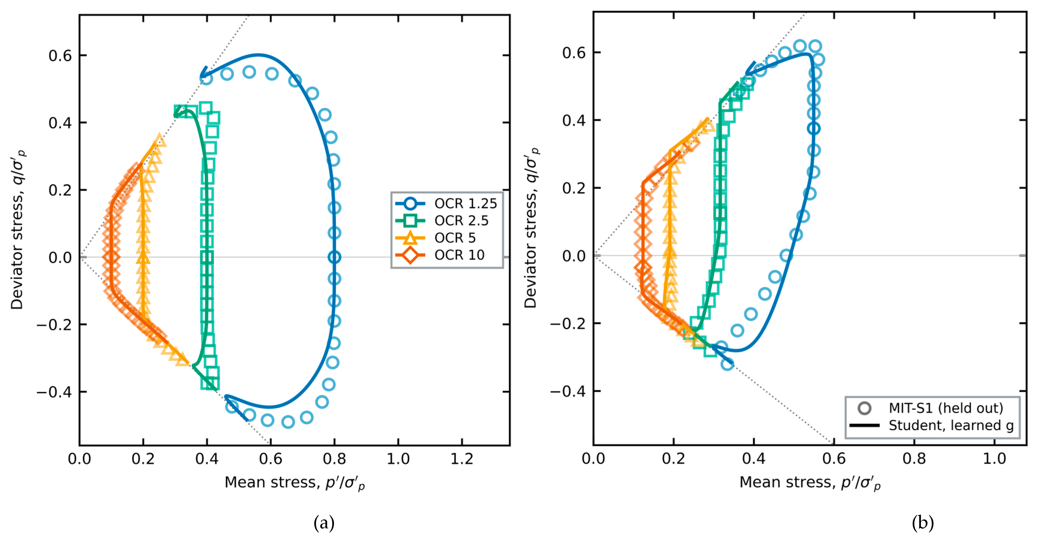
Figure 5.
Undrained strength, student against MIT-S1, normalized by σ′p. Open markers: test paths; small filled markers: training paths. Blue circles: isotropic consolidation (compression and extension); green triangles: K0 consolidation, compression; red squares: K0 consolidation, extension. Solid line: equality; dotted lines: ±10%. (a) Split A; (b) split B, in which no CK0UE path was used in fitting.
Figure 5.
Undrained strength, student against MIT-S1, normalized by σ′p. Open markers: test paths; small filled markers: training paths. Blue circles: isotropic consolidation (compression and extension); green triangles: K0 consolidation, compression; red squares: K0 consolidation, extension. Solid line: equality; dotted lines: ±10%. (a) Split A; (b) split B, in which no CK0UE path was used in fitting.
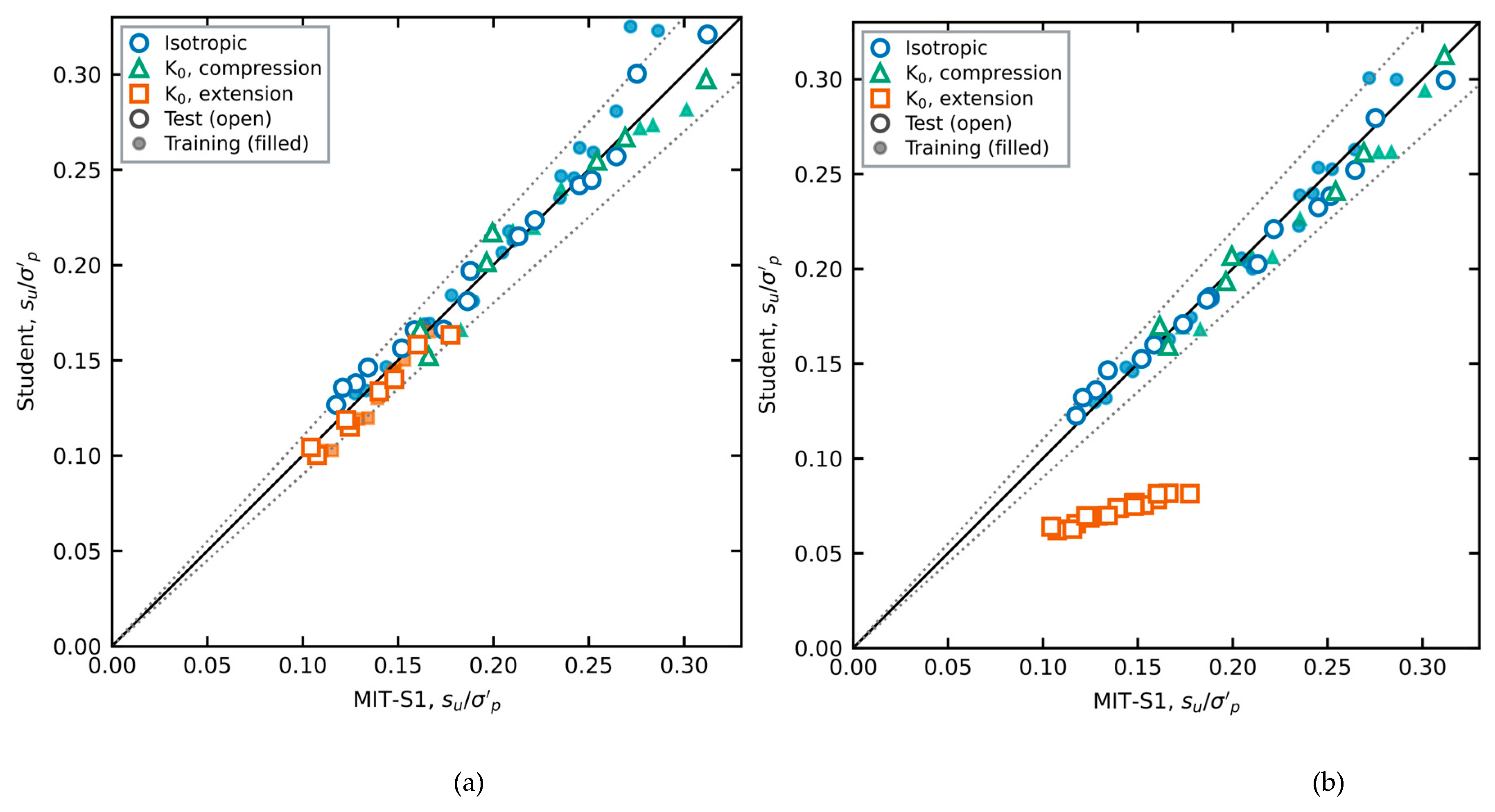
Figure 8.
Dilatancy prescribed by the learned potential (split A, stage S8) against η for R = 1 (blue solid line), 0.5 (green dashed line) and 0.25 (orange dash-dotted line). (a) Isotropic fabric, α = 0; (b) K0 fabric, α = 0.77. The region |η*| < 0.06 (η* = η − cα α), where the two branches are blended, is omitted; for K0 fabric it lies near η = 0.49.
Figure 8.
Dilatancy prescribed by the learned potential (split A, stage S8) against η for R = 1 (blue solid line), 0.5 (green dashed line) and 0.25 (orange dash-dotted line). (a) Isotropic fabric, α = 0; (b) K0 fabric, α = 0.77. The region |η*| < 0.06 (η* = η − cα α), where the two branches are blended, is omitted; for K0 fabric it lies near η = 0.49.
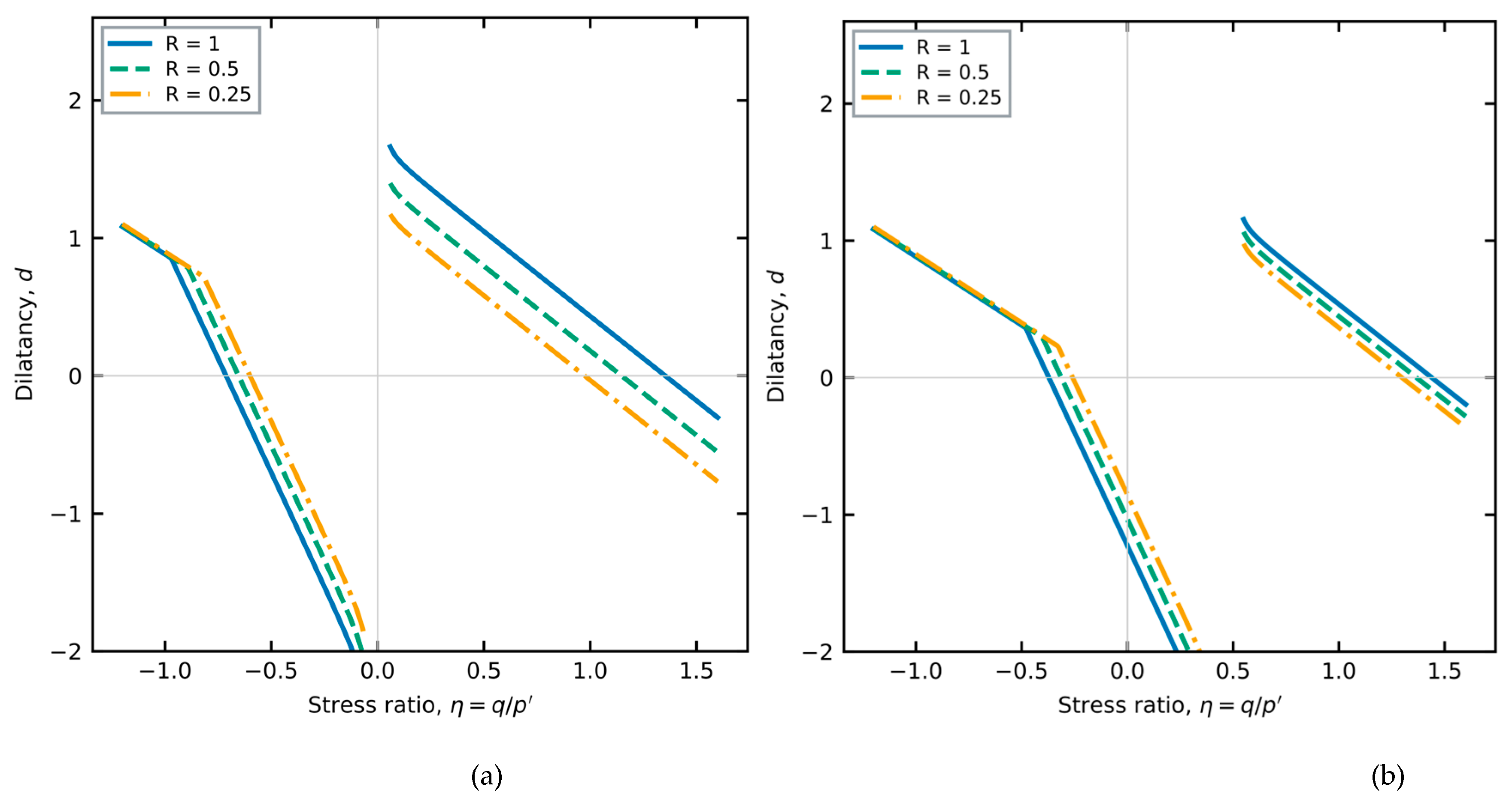
Figure 9.
Peak and post-peak softening in undrained compression of normally consolidated K0 clay: MIT-S1 (open circles), final model (blue solid line) and the softening variant with ξ = 1.5 (red dashed line). (a) σ′p = 4 pa (training path); (b) σ′p = 8 pa (held out).
Figure 9.
Peak and post-peak softening in undrained compression of normally consolidated K0 clay: MIT-S1 (open circles), final model (blue solid line) and the softening variant with ξ = 1.5 (red dashed line). (a) σ′p = 4 pa (training path); (b) σ′p = 8 pa (held out).
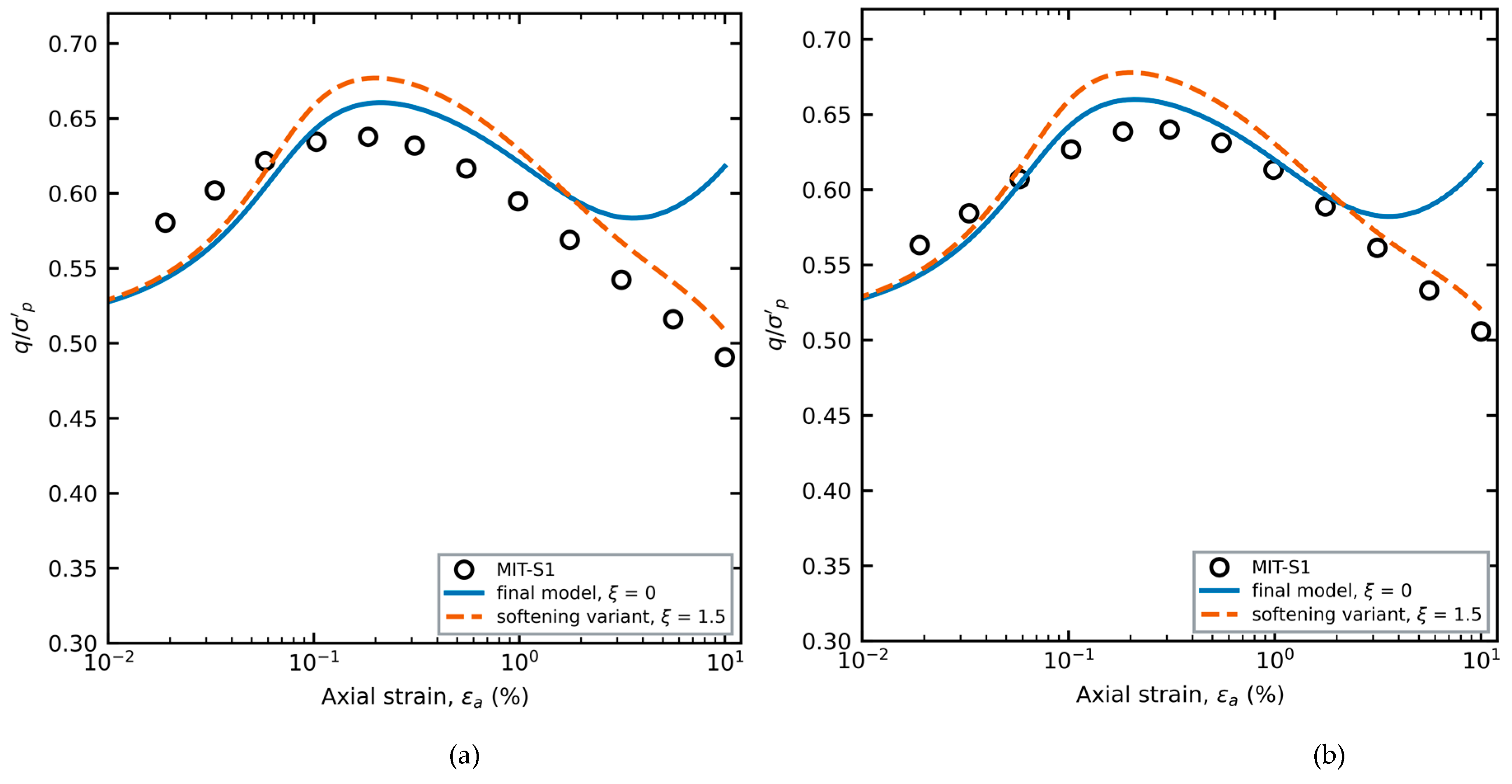
Figure 10.
Undrained strength against OCR, laboratory data (open markers), MIT-S1 (teacher) and the student. (a) Boston Blue Clay, CK0UC: data of Sheahan (circles) and Fayad (squares) as compiled in [8]; teacher (green line); final student of split A (blue line with triangles). (b) Lower Cromer Till: data of Gens compiled in [8] for CK0UC (blue circles), CIUC (red squares) and CIUE (orange triangles); teacher (dotted lines); student with the BBC potential and hardening exponent frozen (solid lines).
Figure 10.
Undrained strength against OCR, laboratory data (open markers), MIT-S1 (teacher) and the student. (a) Boston Blue Clay, CK0UC: data of Sheahan (circles) and Fayad (squares) as compiled in [8]; teacher (green line); final student of split A (blue line with triangles). (b) Lower Cromer Till: data of Gens compiled in [8] for CK0UC (blue circles), CIUC (red squares) and CIUE (orange triangles); teacher (dotted lines); student with the BBC potential and hardening exponent frozen (solid lines).
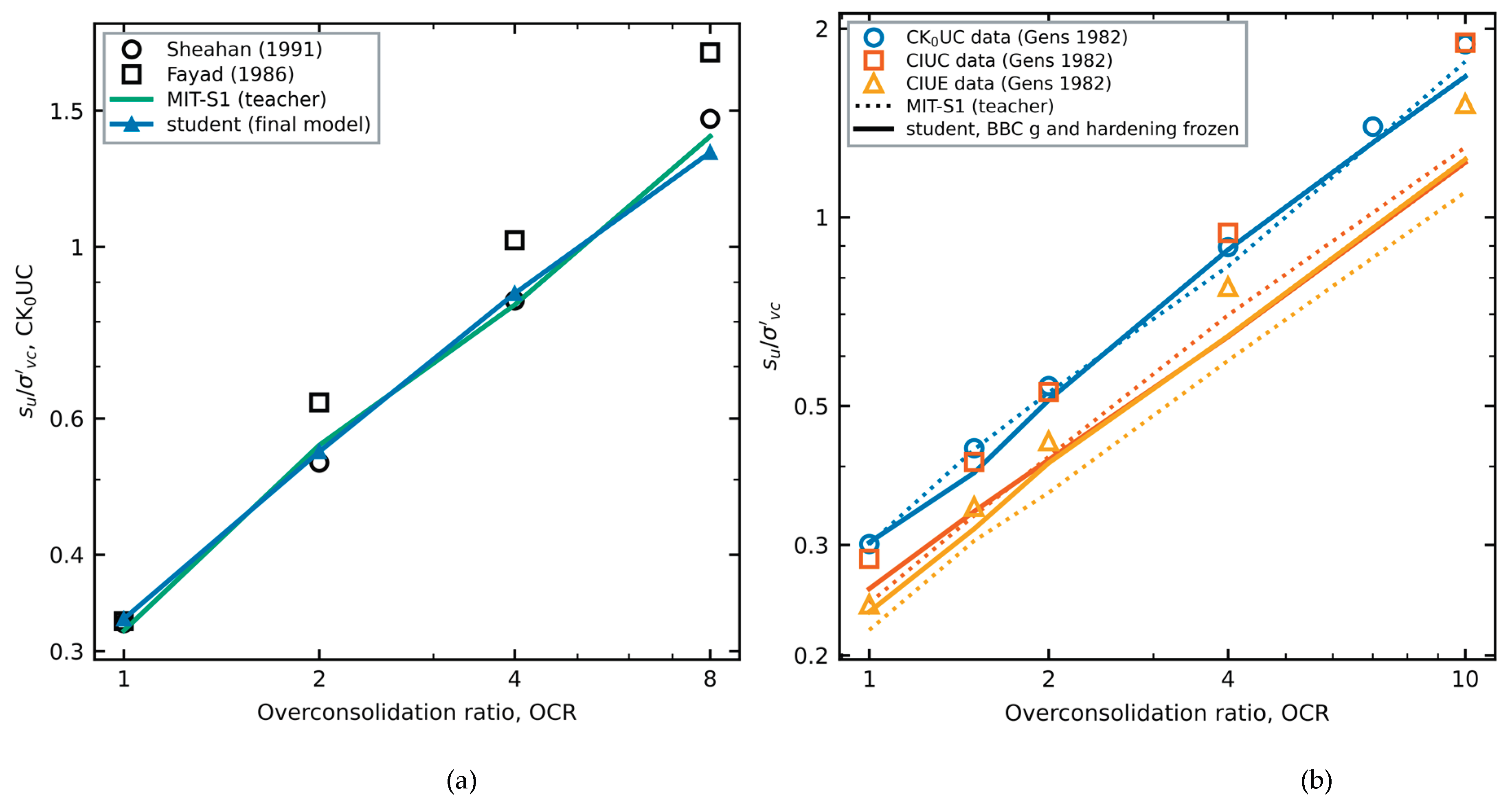
Figure 11.
Four clays: laboratory undrained effective stress paths and predictions with published constants, normalized by the consolidation stress. Markers: data (filled: the one test used to calibrate Ψ and Ω; open: predicted). Solid lines: model extracted from BBC (S8 potential and hardening exponent, frozen); dashed lines: reference AJOP-T. Model curves are drawn to the largest measured strain or, where strains were not reported, to the point nearest the last measurement, as in the error measures. (a) Fujinomori clay; (b) kaolin (five of ten tests shown); (c) Eastern Osaka clay; and (d) weathered Bangkok clay, where the normalized paths of the four tests coincide and one line per model is drawn.
Figure 11.
Four clays: laboratory undrained effective stress paths and predictions with published constants, normalized by the consolidation stress. Markers: data (filled: the one test used to calibrate Ψ and Ω; open: predicted). Solid lines: model extracted from BBC (S8 potential and hardening exponent, frozen); dashed lines: reference AJOP-T. Model curves are drawn to the largest measured strain or, where strains were not reported, to the point nearest the last measurement, as in the error measures. (a) Fujinomori clay; (b) kaolin (five of ten tests shown); (c) Eastern Osaka clay; and (d) weathered Bangkok clay, where the normalized paths of the four tests coincide and one line per model is drawn.
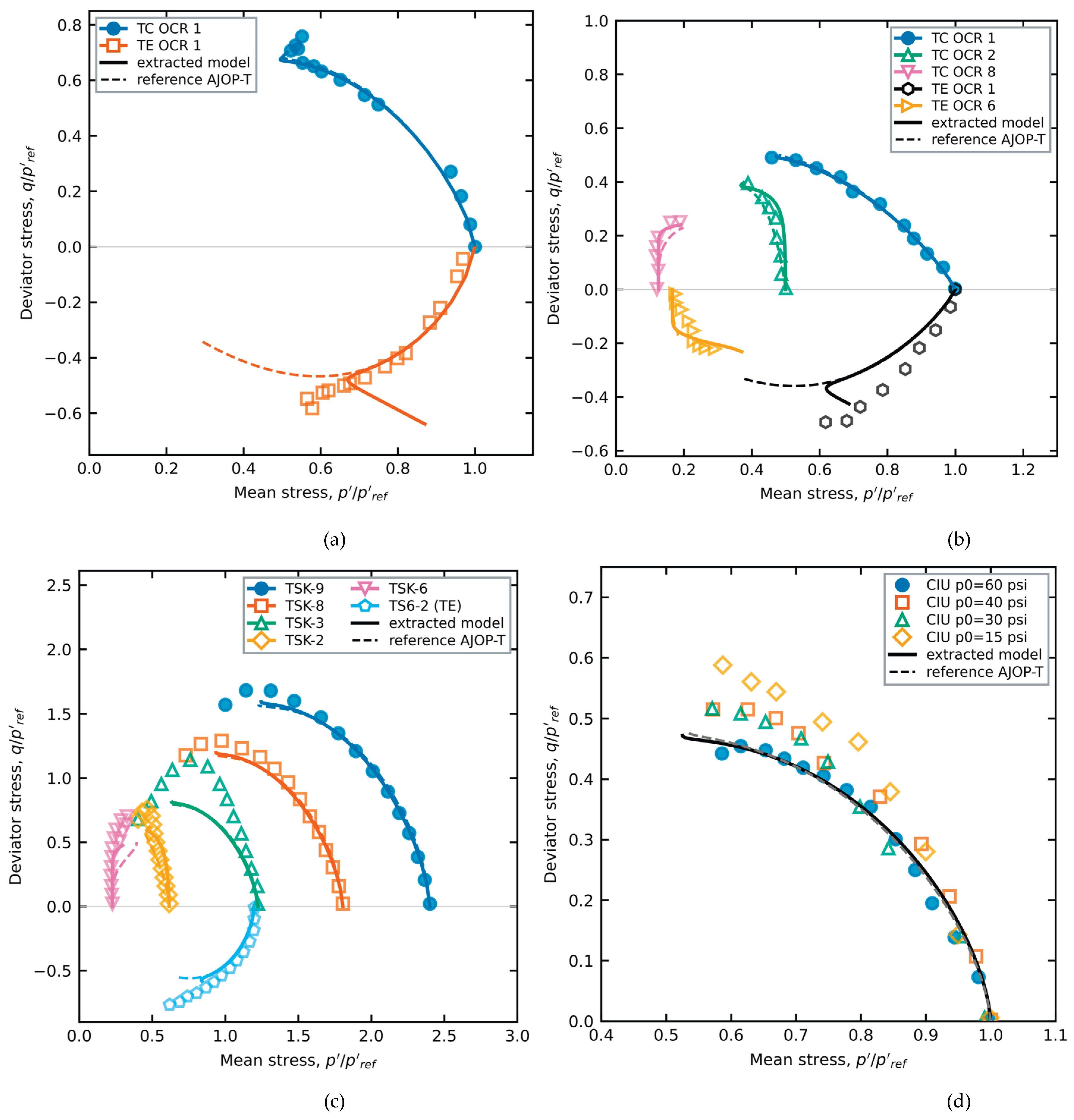
Figure 12.
London Clay: laboratory undrained effective stress paths (data of Gasparre, as compiled in [20]) and predictions, normalized by the consolidation stress. The test at OCR = 1 (filled markers) calibrates Ψ and Ω; the tests at OCR = 2, 6 and 18.7 (open markers) are predicted. Solid lines: model extracted from BBC; dashed lines: reference AJOP-T; curves drawn as in Figure 11.
Figure 12.
London Clay: laboratory undrained effective stress paths (data of Gasparre, as compiled in [20]) and predictions, normalized by the consolidation stress. The test at OCR = 1 (filled markers) calibrates Ψ and Ω; the tests at OCR = 2, 6 and 18.7 (open markers) are predicted. Solid lines: model extracted from BBC; dashed lines: reference AJOP-T; curves drawn as in Figure 11.
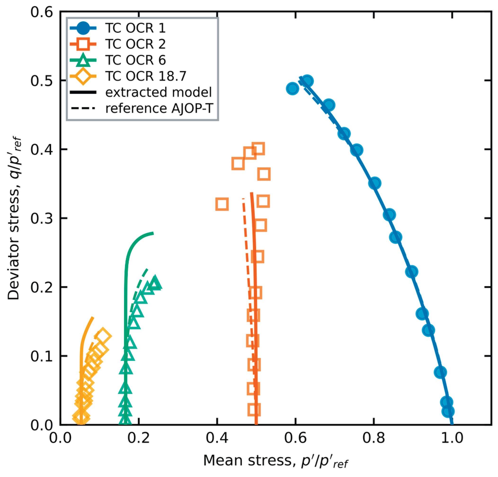
Figure 13.
Undrained strength of isotropically consolidated Lower Cromer Till against OCR: laboratory data of Gens compiled in [8] (open markers), MIT-S1 (dotted lines) and the student of split K (solid lines), which was trained without any isotropic path. Red squares: CIUC; orange triangles: CIUE.
Figure 13.
Undrained strength of isotropically consolidated Lower Cromer Till against OCR: laboratory data of Gens compiled in [8] (open markers), MIT-S1 (dotted lines) and the student of split K (solid lines), which was trained without any isotropic path. Red squares: CIUC; orange triangles: CIUE.
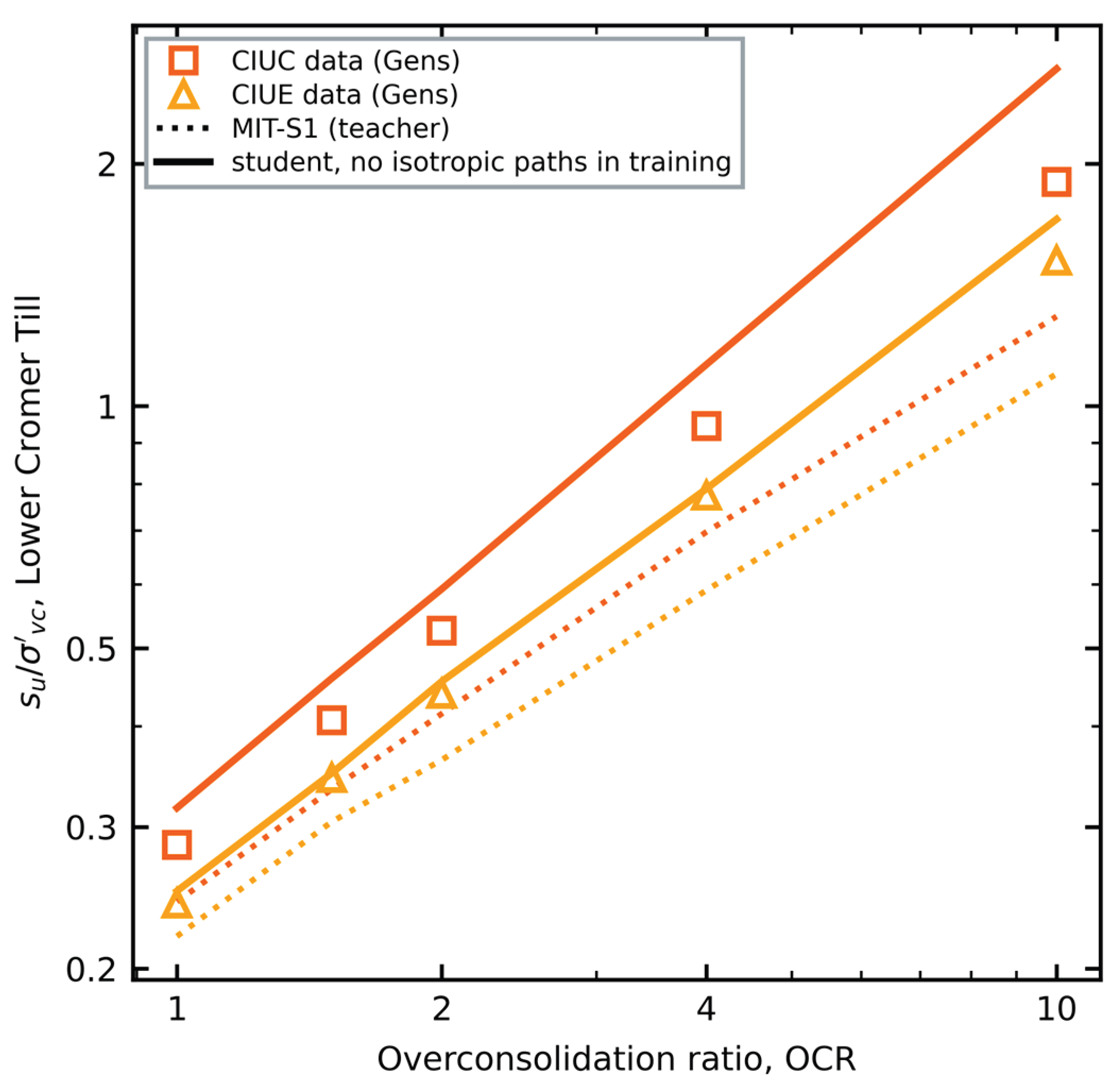
Table 1.
Designs of the study: the question each answers, and its training and test data.
| Design | Question | Training data | Test data | Section |
| Split A | Can the student reproduce the teacher? | MIT-S1/BBC, 96 paths, four families, σ′p = 2, 3, 4, 6 pa | 32 paths: OCR 1.25–5 and 10, σ′p = 8 pa | 3.1–3.7 |
| Split B | Is extension of K0 clay identifiable from compression data? | Split A without any CK0UE path | 19 CK0UE paths | 3.4 |
| Splits C, D | How many extension tests are needed? | Split B plus one (C) or two (D) CK0UE paths | 18 (C) or 17 (D) other CK0UE paths | 3.4 |
| Second teacher | Does the extracted model transfer to another clay? | MIT-S1/LCT, split A roles | LCT test paths | 3.8 |
| Laboratory clays | Does it transfer to real clays? | Model of split A, frozen; Ψ, Ω from one NC test per clay | Laboratory paths of BBC, LCT and five clays | 3.9, 3.10 |
| Split K | Can a student correct its teacher? | MIT-S1/LCT, K0 paths only | Laboratory CIUC, CIUE strengths of LCT | 3.11 |
| Generator | Does learning from many clays transfer better? | 12 synthetic MIT-S1 clays + BBC split A (round 1); 20 clays (round 2) | Five laboratory clays; BBC test paths | 3.12 |
Families: CIUC, CIUE, CK0UC, CK0UE. Selection in every design: lowest validation loss.
Table 2.
MIT-S1 input parameters for Boston Blue Clay (from Table 6.2 of [8]) and simulation inputs.
| Symbol | Meaning | Value |
| ρc | Compressibility at large stresses | 0.178 |
| Cb | Small-strain bulk stiffness constant | 450 |
| 2G/K (μ′₀) | Elastic stiffness ratio (Poisson ratio at small strain) | 1.258 (0.24) |
| K0NC | K0 in normally consolidated state | 0.49 |
| φ′cs | Critical-state friction angle | 33.5° |
| m | Yield-surface shape | 0.80 |
| φ′m | Peak-surface friction angle | 46.0° |
| ψ | Rotational hardening rate | 15 |
| r, D | Swelling (unloading) parameters | 0.85, 0.04 |
| ω, ωs | Small-strain non-linearity | 1.0, 8.0 |
| h | Bounding-surface hardening exponent | 6.0 |
| σ′p, e₀ | Preconsolidation stress, initial void ratio (approximate) | 4 pa, 0.845 |
pa = 100 kPa. The parameter meanings follow [8]; σ′p and e₀ are not stated for the simulated tests and were taken as described in Section 2.2.
Table 3.
Teacher dataset and pre-declared splits (82 original trajectories and 56 added before the final stages).
Table 3.
Teacher dataset and pre-declared splits (82 original trajectories and 56 added before the final stages).
| Family | σ′p (pa) | OCR | Split A role | Split B role |
| CK0UC, CIUC, CIUE | 4 | 1, 1.5, 2, 3, 4, 8 | train | train |
| CK0UC, CIUC, CIUE | 4 | 6 | validation | validation |
| CK0UC, CIUC, CIUE | 4 | 1.25, 2.5, 5 | test-I | test-I |
| CK0UC, CIUC, CIUE | 4 | 10 | test-X | test-X |
| CK0UC, CIUC, CIUE | 2 | 1, 2, 4, 8 | train | train |
| CK0UC, CIUC, CIUE | 8 | 1, 2, 4, 8 | test-S | test-S |
| All four | 3, 6 | 1, 1.5, 2, 3, 4, 6, 8 | train (added) | train (CK0UE: not used) |
| CK0UE | 2, 4, 8 | as above | as above | test (unseen mode) |
| Oedometer | 16 → 32 | 1.5–8 | not used | not used |
Undrained shearing to |εa| = 10%. CK0U: K0 consolidation and swelling; CIU: isotropic. C, E: triaxial compression, extension.
Table 4.
Test performance after each stage of the fitting protocol (split A unless stated). Pass: percentage of test paths with NRMSE < 10% or |su error| < 10%, respectively.
Table 4.
Test performance after each stage of the fitting protocol (split A unless stated). Pass: percentage of test paths with NRMSE < 10% or |su error| < 10%, respectively.
| Stage | Change | CIU NRMSE (pass) | CIU |su err| (pass) | CK0U NRMSE (pass) | CK0U |su err| (pass) | Flow mismatch |
| S1 | Student constants re-fitted (Adam) | 0.085 (75%) | 27.8% (31%) | 0.078 (81%) | 41.2% (12%) | 17° |
| S2 | + strain-dependent swelling index, Eq. (5) | 0.065 (100%) | 24.9% (31%) | 0.050 (94%) | 16.4% (31%) | 17° |
| S3 | + Nova-type potential, AC0, AE0, βC0, βE0 | 0.069 (94%) | 15.4% (31%) | 0.058 (100%) | 14.7% (31%) | 27° |
| S4 | + fabric terms γ; all constants by CMA-ES | 0.036 (100%) | 6.6% (81%) | 0.042 (94%) | 7.2% (81%) | 21° |
| S4-O | as S4, g = g0 at α = 0 (constrained) | 0.042 (94%) | 10.3% (81%) | 0.049 (94%) | 13.1% (44%) | 19° |
| S5 | + flow-direction term (w = 0.1), ν ∈ [0.15, 0.35] | 0.041 (100%) | 5.9% (75%) | 0.039 (100%) | 8.5% (75%) | 10° |
| S6 | + kE, cE | 0.042 (100%) | 7.7% (69%) | 0.041 (94%) | 7.5% (75%) | 10° |
| S6-B | S6 protocol, split B (excluding unseen CK0UE) | 0.044 (100%) | 2.6% (100%) | 0.041 (100%) | 6.8% (62%) | 9° |
| S7 | + learned hardening exponent and starting fabric, Eq. (11); 96 training paths; lowest validation loss of three seeds | 0.037 (100%) | 4.0% (94%) | 0.031 (100%) | 4.1% (100%) | 8° |
| S8 | kinematic potential, Eq. (12); 96 training paths; family-balanced loss; lowest validation loss | 0.036 (100%) | 4.8% (94%) | 0.029 (100%) | 4.3% (100%) | 8° |
| final-B | split B, 72 training paths, lowest validation loss (S7 configuration); unseen CK0UE excluded | 0.033 (100%) | 3.8% (100%) | 0.028 (100%) | 3.3% (100%) | 7° |
All test sets (I, X, S) pooled; 16 CIU and 16 CK0U paths in split A. Flow mismatch: mean angle between student and MIT-S1 plastic strain increments on the same test paths. S6-B row: 16 CIU and 4 CK0UC test paths; the 19 unseen CK0UE paths are reported in Section 3.4.
Table 5.
Fitted constants of the final model (stage S8) for split A and of the final split-B model.
| Constant | Role | Split A | Split B |
| Ψ | surface shape | 3.324 | 2.37 |
| Ω | surface shape | 0.2049 | 0.6751 |
| κ0 | swelling index, small strain | 0.01901 | 0.01446 |
| κ1 | swelling index, large strain | 0.02803 | 0.04559 |
| εr | degradation strain | 0.0623 | 0.02563 |
| ν | Poisson ratio | 0.15 | 0.15 |
| ac | AJOP slope | 0.1202 | 0.06574 |
| θc | AJOP roundness | 55.49 | 0.5143 |
| pr (pa) | AJOP reference stress | 0.8776 | 0.3579 |
| ω | rotation rate | 120.4 | 26.55 |
| ωd | deviatoric rotation | 10.18 | 0.1332 |
| AC0 | dilatancy slope, compression | 1.228 | 1.018 |
| AE0 | dilatancy slope, extension | 3.303 | 2.028 |
| βC0 | R-exponent, compression | 0.2371 | 0.1069 |
| βE0 | R-exponent, extension | 0.124 | 0.09783 |
| γA,C | fabric effect on AC | −0.01852 | 0.1661 |
| γA,E | fabric effect on AE | 0 | 0.2777 |
| γβ,C | fabric effect on βC | −0.2775 | −0.6783 |
| γβ,E | fabric effect on βE | 0 | 0.2921 |
| kE | extension critical ratio factor | 0.764 | 0.9207 |
| cE | extension rotation target | 1 | 1.376 |
| cα | kinematic shift of the potential, Eq. (12) | 0.636 | – |
| h0 | hardening exponent, constant | 1.718 | 1.582 |
| h1 | hardening exponent, R term | 8.396 | 4.718 |
| h2 | hardening exponent, fabric term | 1.044 | −0.6111 |
| h3 | starting fabric exponent | −0.04734 | 0.4587 |
| h4 | hardening exponent, (1 − R)² term | −0.7277 | 1.411 |
M = 1.353 (from φ′cs = 33.5°) and e0 = 0.845 are fixed. The two calibrations predict the shared test paths with similar accuracy, which shows that the constants are not uniquely identified (Section 3.5).
Table 7.
Laboratory stress paths of five clays: published constants, Ψ and Ω calibrated on one normally consolidated compression test, all other tests predicted. Reference: AJOP-T with g₀ and the reference hardening exponent. Extracted: S8 potential and hardening exponent from BBC, frozen. Means over predicted tests.
Table 7.
Laboratory stress paths of five clays: published constants, Ψ and Ω calibrated on one normally consolidated compression test, all other tests predicted. Reference: AJOP-T with g₀ and the reference hardening exponent. Extracted: S8 potential and hardening exponent from BBC, frozen. Means over predicted tests.
| Clay (source) | Tests predicted | Model | Ψ, Ω | ESP-RMSE | q–ε RMSE | |peak su| error |
| Fujinomori [22] | 1 | reference | 1.35, 1.10 | 0.051 | 0.124 | 19.7% |
| extracted | 1.35, 1.10 | 0.063 | 0.045 | 9.6% | ||
| Kaolin [64] | 9 | reference | 1.13, 0.85 | 0.042 | 0.060 | 13.3% |
| extracted | 1.13, 0.85 | 0.025 | 0.033 | 13.4% | ||
| Eastern Osaka [70] | 5 | reference | 1.58, 1.25 | 0.096 | – | 23.3% |
| extracted | 1.50, 1.30 | 0.088 | – | 22.3% | ||
| Weathered Bangkok [71] | 3 | reference | 1.50, 1.25 | 0.050 | 0.071 | 10.7% |
| extracted | 1.54, 1.25 | 0.051 | 0.088 | 11.6% | ||
| London [20] | 3 | reference | 1.28, 1.19 | 0.018 | – | 11.9% |
| extracted | 1.24, 1.25 | 0.029 | – | 24.0% |
ESP-RMSE and q–ε RMSE normalized by the consolidation stress; q–ε RMSE only for tests with reported strains; for weathered Bangkok clay the column gives the RMSE of η = q/p′ against shear strain, as reported in the source. Peak strength compared within the measured range of each test. Fabric off.
Table 8.
Whole-curve errors on the laboratory clays: mean ESP-RMSE / mean q–ε RMSE (where strains were reported) over the predicted tests.
Table 8.
Whole-curve errors on the laboratory clays: mean ESP-RMSE / mean q–ε RMSE (where strains were reported) over the predicted tests.
| Clay | Reference AJOP-T | Single teacher (BBC) | Generator, round 1 | Generator, round 2 |
| Fujinomori | 0.051 / 0.124 | 0.063 / 0.045 | 0.057 / 0.044 | 0.052 / 0.042 |
| Kaolin | 0.042 / 0.060 | 0.025 / 0.033 | 0.025 / 0.033 | 0.025 / 0.033 |
| Eastern Osaka | 0.096 | 0.088 | 0.087 | 0.086 |
| Weathered Bangkok | 0.050 / 0.071 | 0.051 / 0.088 | 0.048 / 0.106 | 0.052 / 0.102 |
| London | 0.018 | 0.029 | 0.028 | 0.029 |
Disclaimer/Publisher’s Note: The statements, opinions and data contained in all publications are solely those of the individual author(s) and contributor(s) and not of MDPI and/or the editor(s). MDPI and/or the editor(s) disclaim responsibility for any injury to people or property resulting from any ideas, methods, instructions or products referred to in the content. |
© 2026 by the authors. Licensee MDPI, Basel, Switzerland. This article is an open access article distributed under the terms and conditions of the Creative Commons Attribution (CC BY) license (http://creativecommons.org/licenses/by/4.0/).
Copyright: This open access article is published under a Creative Commons CC BY 4.0 license, which permit the free download, distribution, and reuse, provided that the author and preprint are cited in any reuse.