

Submitted:
13 November 2026
Posted:
17 November 2026
You are already at the latest version
Abstract
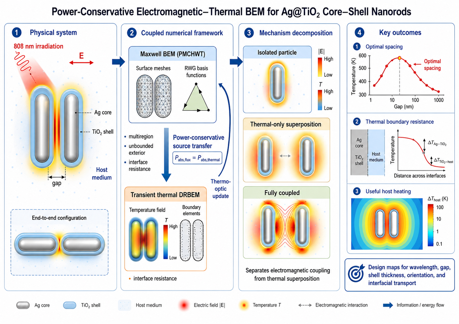
Thermoplasmonic core shell nanostructures provide an effective platform for localized optical heating, but accurate prediction of their thermal response requires a computational framework capable of distinguishing electromagnetic interactions from thermal field superposition while accounting for heat transfer across material interfaces. This study develops a three dimensional multiregion boundary element formulation and verification protocol for silver titanium dioxide core shell nanostructures embedded in an unbounded host medium. The electromagnetic problem is formulated using a surface integral representation with Rao Wilton Glisson discretization, allowing multiple material interfaces and exterior radiation conditions to be treated directly. Optical absorption is independently evaluated through volumetric electromagnetic loss and boundary Poynting flux, providing a consistent and auditable transfer of absorbed optical energy to the thermal model. Transient heat conduction is formulated through a modified Helmholtz representation and solved using a dual reciprocity boundary element approach that incorporates finite thermal boundary resistance at the silver titanium dioxide and titanium dioxide host interfaces. A controlled decomposition procedure is introduced to distinguish temperature changes caused by thermal field overlap from those associated with electromagnetic modification of optical absorption. Verification is supported through sphere based electromagnetic controls, analytical transient thermal benchmarks, interface resistance assessment, and reconstruction of a published reference geometry. The study establishes a reproducible and conservation based computational framework for the rigorous analysis of coupled electromagnetic and thermal transport in coated plasmonic nanostructures, with emphasis on numerical consistency, energy conservation, interfacial effects, source transfer accuracy, and systematic verification before predictive nanoscale simulations are undertaken.
Keywords:
boundary element method
; thermoplasmonics
; core shell nanorods
; optical thermal coupling
; thermal boundary resistance
; verification protocol
1. Introduction
Thermoplasmonic nanomaterials harvest optical energy as localized heat and thus provide a controlled means of photothermal treatment, catalytic activity, nanoscale chemistry, optical manipulation, and localized thermal sensing. The usefulness of a plasmonic heater is not just because a metallic nanoparticle can absorb light; rather, it is that resonant field concentration can deposit energy within a volume far smaller than the free-space wavelength. The temperature response, however, is governed by a chain of coupled processes: electromagnetic excitation establishes the internal loss density, electron and lattice subsystems equilibrate, heat crosses material interfaces, and thermal diffusion redistributes the deposited energy into the surrounding medium. Foundational thermoplasmonic analyses established the relation between morphology, optical absorption, and nanoscale heating [1,2], while later work on nanoparticle arrays demonstrated that the experimentally observed temperature can be dominated by collective thermal accumulation rather than by the response of an isolated particle [3]. Transient analyses further showed that pulse duration, array size, observation time, and interparticle spacing jointly determine whether a nanoparticle ensemble behaves as a set of independent heat sources or as a collective thermal body [4]. These observations make clear that a useful model must conserve optical power, resolve material interfaces accurately, and distinguish local absorption changes from subsequent thermal-field overlap.
Interparticle separation is especially important because electromagnetic and thermal interactions obey different length and time scales. Plasmonic coupling is highly sensitive to polarization, particle orientation, resonance detuning, and the normalized gap, and its distance dependence has been quantified through the plasmon-ruler concept [5]. By contrast, temperature fields diffuse beyond the optical near-field region and can overlap even when the particles are too widely separated for appreciable electromagnetic hybridization. Recent finite-element calculations for Ag–TiO₂ core–shell nanorods reported a non-monotonic spacing dependence that was attributed to competition between electromagnetic coupling and thermal superposition [6]. A related study of TiN–Au core–shell nanorods showed that the photothermal response of a coated anisotropic particle is controlled by both the optical resonance of the composite structure and heat transfer through the shell [7]. The central difficulty is therefore interpretive as well as numerical: two particle configurations can produce similar peak temperatures while arriving there through fundamentally different changes in absorbed power, thermal resistance, or heat-field overlap. Without an explicit decomposition, a temperature-versus-gap curve alone cannot identify the physical mechanism responsible for an apparent optimum.
The core–shell architecture introduces additional design freedom but also additional uncertainty. A TiO₂ coating can protect silver from chemical degradation, alter colloidal stability, tune the local dielectric environment, increase the minimum Ag–Ag separation, and modify the spatial distribution of the electric field. The same shell also creates Ag–TiO₂ and TiO₂–host interfaces across which heat must pass. At nanometer dimensions, the temperature drop at an interface need not be negligible, because thermal boundary conductance depends on bonding, roughness, disorder, vibrational mismatch, interfacial chemistry, and the nature of the adjacent liquid or solid [8]. Modern studies of coupled interfacial energy transduction have further emphasized that electrons, phonons, molecules, and polaritonic excitations can contribute on different time scales [9]. Consequently, the hottest metal configuration is not necessarily the configuration that delivers the greatest or most spatially uniform temperature rise to the target medium. A predictive model should therefore report the metal temperature, the shell temperature, the host temperature, the interfacial temperature jumps, and the net outward heat flux rather than relying on a single maximum-temperature metric.
Reliable optical input data are equally important. The Johnson–Christy measurements remain the most widely used reference for the complex permittivity of silver [10], but later ellipsometric measurements and systematic re-evaluations have shown that film quality, grain structure, surface roughness, deposition history, and interpolation procedure can produce meaningful differences in both the real and imaginary parts of the dielectric function [11,12]. These differences influence the wavelength, bandwidth, and absorbed power of resonance. TiO₂ is another factor that contributes to the variability since its optical parameters are dependent on the crystalline form, porosity, stoichiometry, fabrication process, and size of nanocrystals, which may differ from those of bulk anatase/rutile [13]. In a core–shell calculation, an apparently small change in either constituent can shift the composite resonance relative to the prescribed laser wavelength and can change the sign of the electromagnetic contribution to the temperature response. For that reason, optical-property provenance and interpolation must be treated as part of the numerical method, not as incidental input preparation.
Several analytical and numerical frameworks are available for nanoparticle optics. Mie-type solutions provide indispensable verification for homogeneous and concentric spheres, whereas differential and volume-discretization methods are flexible for general geometries [14,15]. Surface-integral formulations are particularly attractive for piecewise homogeneous nanoparticles because they replace volumetric electromagnetic unknowns with equivalent currents on material interfaces and impose the radiation condition through the Green function. The MNPBEM framework demonstrated the practical value of this approach for plasmonic nanoparticles [16], and later hierarchical-matrix and iterative-solver developments extended it to much larger surface systems [17]. Boundary-integral studies of single and coupled metallic nanoparticles also showed that retardation, shape, and particle interaction can be treated directly within a surface formulation [18]. For a coated nanorod assembly embedded in an unbounded host, these features eliminate the artificial exterior truncation and absorbing layers required by most domain methods, while concentrating spatial resolution on the core–shell boundary, the shell–host boundary, and the narrow interparticle gap.
A full-wave treatment of penetrable metallic and dielectric regions requires careful multiregion assembly. The Poggio–Miller–Chang–Harrington–Wu–Tsai formulation combines tangential electric- and magnetic-field integral equations and provides a common representation for composite dielectric–metallic structures. Its extension to general junctioned configurations has been developed within surface-integral equation frameworks [19]. Nevertheless, direct discretization can become poorly conditioned as the mesh is refined or as multiple absorbing particles interact; Calderón-based and strong-form preconditioners have therefore been investigated for single- and multiple-particle PMCHWT systems [20,21]. The surface currents are commonly expanded with Rao–Wilton–Glisson basis functions on pairs of triangular elements [22], and the resulting dense nonsymmetric systems are solved efficiently with Krylov methods such as GMRES [23]. In practical implementations, the most common failures are not abstract theoretical issues but sign and orientation errors at internal interfaces, insufficient treatment of nearly singular gap integrals, inconsistent material-side traces, and power expressions that do not use the same time convention as the field solver. A publication-grade formulation must make these choices explicit and must include optical-theorem and energy-balance tests as routine regression checks.
The thermal problem poses a different challenge because electromagnetic loss is volumetric even when the field problem is solved on surfaces. Dual-reciprocity boundary element methods provide a systematic way to approximate nonhomogeneous source terms by radial basis functions and convert their effect into boundary quantities [24]. Isogeometric and higher-order developments have demonstrated the applicability of this strategy to transient heat conduction with distributed sources [25]. Classical time-dependent boundary integral formulations remain valuable for analytical verification and for understanding the treatment of the initial condition [26], while nonlinear extensions show how temperature-dependent properties and nonhomogeneous heat sources can be incorporated [27]. For thermoplasmonic particles, the key implementation requirement is a conservative transfer of the electromagnetic loss field to the thermal source representation. If the transferred source does not reproduce the independently computed absorbed power, excellent-looking temperature contours can still be quantitatively wrong. Source fitting, regional power conservation, time-step convergence, and interfacial flux continuity must therefore be verified separately.
Additional formulations become relevant when particles approach the extreme nanoscale. Parallel advances in boundary-integral heat-transfer modelling have demonstrated that nonclassical transport mechanisms, including multi-term fractional heat conduction in heterogeneous media and size-dependent micropolar porous thermoelasticity with non-Fourier heat conduction, can be incorporated without abandoning the boundary-based computational framework [28,29]. Field-only surface integral equations can remove explicit surface-current unknowns and provide alternative regularization strategies for dielectric scattering [30]. Mesoscopic boundary conditions based on surface-response parameters allow nonclassical interface effects to be incorporated into a BEM without volumetric quantum calculations [31]. For subnanometre metallic gaps, quantum-corrected models can represent tunnelling-mediated charge transfer and the associated modification of plasmon modes [32]. The present reference geometries lie predominantly in the local classical regime because the metal surfaces are separated by the dielectric shell and the investigated shell-to-shell gaps are much larger than a tunnelling distance. Nevertheless, clearly stating the validity range is essential: a classical local-response result should not be extrapolated to atomic-scale gaps merely by refining the mesh.
Despite substantial progress in thermoplasmonic modeling, a unified boundary-based formulation remains useful for coated anisotropic particles when the exterior optical and thermal domains are unbounded, all material interfaces are represented explicitly, optical power is evaluated by independent expressions, transient volumetric heating is transferred without uncontrolled gain or loss, thermal boundary resistance is permitted at both interfaces, and electromagnetic coupling is separated conceptually from thermal superposition. Existing finite-element studies provide valuable physical benchmarks [6,7], whereas a surface formulation offers a complementary route in which interface quantities and exterior radiation or decay conditions are represented directly. The contribution pursued here is therefore methodological: it defines the coupled equations, the region–interface assembly, the source-transfer audit, and the verification sequence required before predictive design calculations are attempted.
In this paper, a three-dimensional multiregion boundary-element formulation is specified for thermoplasmonic Ag–TiO₂ core–shell nanostructures. The electromagnetic problem is written in region–interface incidence form using PMCHWT operators intended for RWG Galerkin discretization with singular and near-singular quadrature. Optical absorption is defined independently by volumetric loss and boundary Poynting flux so that electromagnetic-to-thermal source transfer can be audited. The transient heat equation is recast as a fixed-step BDF2 modified-Helmholtz problem with a dual-reciprocity representation of volumetric heating, and imperfect Ag–TiO₂ and TiO₂–host thermal contact is imposed through explicit temperature-jump conditions. A three-calculation decomposition is defined to distinguish thermal-field overlap from electromagnetic modification of absorption. Thermo-optic feedback is retained only as a prospective extension.
The evidence status is explicit throughout this revision: Section 3, Section 4, Section 5, Section 6, Section 7 and Section 8 define the mathematical formulation, reference implementation choices, and required verification workflow, whereas Section 9 reports only the controls that were actually executed. Full-wave PMCHWT–RWG sphere and nanorod calculations, numerical transient DRBEM validation, dimer gap sweeps, measured power-balance residuals, and thermo-optic iterations are not presented as completed results.
The remainder of the article is organized as follows. Section 2 defines the geometry, material data, illumination, scale separation, and evidence scope. Section 3 states the governing equations and coupling definitions. Section 4 and Section 5 derive the multiregion electromagnetic and transient thermal BEM formulations. Section 6 distinguishes the one-way baseline from the prospective thermo-optic extension. Section 7 and Section 8 provide a reference implementation specification and the verification requirements for a complete solver. Section 9 contains the reported analytical, low-frequency, and benchmark-reconstruction controls. Section 10 and Section 11 discuss only conclusions supported by those reported data.
2. Materials and Methods
The study is organized so that geometry, material data, boundary-integral assembly, source transfer, and verification obligations can be audited independently. The finite-element configuration of Pu et al. [6] is reconstructed as an external reference geometry and source of validation targets; no BEM–FEM agreement is claimed in the absence of completed full-wave and transient-BEM output. The calculations actually reported in this article are limited to the electrostatic sphere control, analytical transient-thermal control, equivalent-resistance screening, and benchmark-geometry reconstruction. The remaining numerical procedures are presented as a reference implementation and verification protocol for a complete solver.
Table 1 compares the computational implications of the principal numerical strategies and identifies the specific capabilities required for the present core–shell thermoplasmonic problem.
2.1. Geometry and Material Regions
Each particle consists of an Ag core occupying Ω1 and a TiO2 shell occupying Ω2. The unbounded surrounding medium occupies Ω0. The core–shell interface is Γ12 and the shell–host interface is Γ20. For multiple particles, the same notation is augmented by a particle index. The reference Ag core is a spherocylinder of total length L = 62 nm and diameter
with shell thickness ts = 10 nm. The corresponding outer dimensions are Lo = L + 2ts = 82 nm and Do = D + 2ts = 42.14 nm. The geometric convention is shown in Figure 1. The reported distance in all calculations is the minimum shell-to-shell gap. This convention removes an ambiguity that otherwise arises in dimer studies, where “distance” may refer to center spacing, metal-to-metal spacing, or outer-surface spacing.
Figure 1 establishes the geometric and illumination conventions used throughout the study, including the Ag core, TiO2 shell, reference normals, and the distinct shell-to-shell gaps for side-by-side and end-to-end configurations.
Figure 2 illustrates the surface-discretization strategy used for close particle pairs. The opposing surfaces are refined independently of the remote particle surfaces so that gap accuracy is not determined by the global mesh density.
For side-by-side rods, the center-to-center distance is dc = Do + g. For end-to-end rods, it is dc = Lo + h. Arbitrary orientations are described by a rotation matrix Rp ∈ SO(3) for particle p and a translation vector xp. No symmetry plane is assumed in the general implementation.
2.2. Optical and Thermal Properties
Each region is homogeneous, isotropic, and nonmagnetic, with μr = μ0 unless otherwise stated. The complex electric permittivity is
For the baseline optical definition, silver is referenced to the Johnson–Christy optical constants [10], and TiO₂ is referenced to the experimentally characterized data source cited as Ref. [13]. The host refractive index used in the reconstructed reference problem is n0 = 1.44, following Ref. [6]. Because no full wave optical result is reported in Section 9, the present article does not infer missing phase specific or temperature dependent optical data. For a future full wave implementation following this protocol, the exact sampled optical tables must be archived; the reference interpolation prescription is piecewise linear in wavelength for n and κ separately, with no extrapolation outside the tabulated range.
The baseline thermal properties follow Ref. [6] and are summarized in Table 2. They reproduce the reference-model inputs rather than universal nanoscale values. The Ag–TiO₂ and TiO₂–host thermal boundary resistances are treated as uncertain parameters. The interval explored in Section 9.5 is deliberately a broad screening interval, not a measured interface-specific prior. References [8,9] support the sensitivity of nanoscale thermal boundary conductance to bonding, roughness, disorder, chemistry, and adjacent media, but the present paper does not assign a measured Ag–TiO₂ or TiO₂–host resistance distribution.
Table 2 consolidates the baseline thermophysical inputs used only to reproduce the reference configuration; the values should be replaced by measured or uncertainty-bounded properties when predictive nanoscale claims are made.
2.3. Illumination and Initial State
The incident field is a monochromatic plane wave with angular frequency ω = 2πc0/λ0,
where , , and the time convention is e−iωt. The irradiance is
The particular choice of parameters for the reference problem takes the values of λ0 = 808 nm, I0 = 2.5 × 10⁸ W m−2, n0 = 1.44 and T0 = 310 K. The laser envelope p(t) is normalized to the condition 0 ≤ p(t) ≤ 1. Constant heating corresponds to p(t) = H(t)
2.4. Scale Separation and Model Validity
The optical period at 808 nm is a few femtoseconds, whereas the thermal evolution considered in the reference study occurs over nanoseconds to microseconds. The electromagnetic problem can therefore be solved in the frequency domain and its cycle-averaged dissipation passed to the thermal problem. The model begins after electron-electron and electron-phonon relaxation have produced a meaningful lattice temperature. A two-temperature metal model is required for ultrashort pulses when sub-picosecond electron and lattice temperatures are of interest; it is not required for the continuous-wave and nanosecond-scale regime addressed here.
At the particle scale, tissue perfusion and metabolic heat generation are negligible relative to conduction. A Pennes perfusion term at a characteristic length of 100 nm and a characteristic time of 1 μs changes the solution by an amount far below the material-property uncertainty and is therefore omitted. Perfusion becomes relevant only when the nanoparticle-scale solution is embedded in a larger tissue-domain model over millimeter and second scales. Convection at the particle surface is likewise not imposed as a separate coefficient because the host is solved explicitly as a conductive continuum.
The local classical dielectric model is appropriate for the reference gaps, which are tens of nanometers. If the shell-to-shell or metal-to-metal gap is reduced to roughly 1–2 nm, nonlocal response, electron spill-out, tunneling, ligand layers, and geometric uncertainty can dominate. Such cases cannot be considered quantitatively predictive using an unmodified local PMCHWT model.
Table 3 reports derived geometric and time-scale quantities calculated from the reference inputs. These values are used to select temporal resolution, far-field evaluation distances, and benchmark windows before any parameter sweep is performed.
3. Governing Equations
3.1. Frequency-Domain Maxwell System
In each region Ωr, the total fields satisfy
∇×Er = iωμrHr, ∇×Hr = −iωεrEr.
Eliminating the magnetic field in a homogeneous source-free region gives the vector Helmholtz equation
The square-root branch is chosen so that Imβr ≥ 0 in passive media. On every interface Γab without impressed surface charge or current, tangential fields are continuous:
nab × (Ea − Eb) = 0, nab × (Ha − Hb) = 0.
The exterior scattered field satisfies the Silver–Müller radiation condition,
3.2. Optical Dissipation and Cross-Sections
For the adopted time convention, the cycle-averaged volumetric electromagnetic heat source is
The magnetic-loss term vanishes for the present nonmagnetic media. The absorbed power in a bounded region can be evaluated either by volume integration,
or, more naturally in a boundary method, by the inward time-averaged Poynting flux,
Equation (11) is the preferred global power calculation because it uses only boundary traces. Equation (10) remains useful when a spatially resolved source must be transferred to the thermal solver. The absorption cross-section is
The extinction power follows from the interference of incident and scattered fields on a closed surface in the host, and the scattering power is the outward scattered Poynting flux. The numerical energy residual is
A visually plausible near-field plot is not a substitute for this balance. For a future converged production calculation, the electromagnetic energy residual should be reported over mesh and quadrature refinement and should normally be below 1%, with a more stringent target in the Mie-validation cases. No full-wave value of this residual is reported in the present results.
3.3. Transient Heat Conduction
The temperature in region r satisfies
For constant isotropic kr,
The source is
where Qother,r is zero in the nanoparticle-scale reference model. The initial condition is Tr(x,0) = T0. In the unbounded host,
Qr(x,t) = p(t)QEM,r(x,T) + Qother,r,
T0(x,t) → T∞(t) as |x| → ∞.
For the baseline case, T∞ = 310 K.
3.4. Thermal Interface Resistance
Let nab point from region a to region b, and define the positive heat flux from a to b as
qab = −ka∇Ta ⋅ nab = −kb∇Tb ⋅ nab
Energy conservation and a finite Kapitza resistance Rab give
Ta − Tb = Rabqab.
Perfect thermal contact is recovered with Rab = 0. Retaining separate interface temperatures is essential. A code that merges the Ag and TiO2 temperature degrees of freedom at mesh generation cannot later add thermal boundary resistance without restructuring the formulation.
3.5. Prospective Thermo-Optic Extension
Thermo-optic feedback is not activated in any numerical result reported in this article. Equation (20) is retained as a prospective extension: a future two-way implementation would update the optical material properties from the current temperature field according to
A measured tabulation of temperature-dependent optical data is preferable to a local linearization. Because no such dataset, iteration history, absorbed-power change, or temperature change is reported here, the manuscript makes no claim of demonstrated two-way thermo-optic coupling. When this extension is implemented, the data provenance, calibrated temperature interval, interpolation rule, under-relaxation factor, and convergence history must be reported.
3.6. Coupling-Decomposition Measures
Three simulations are used at each geometry. The isolated-particle case gives Qsingle and ΔTsingle. The thermal-only dimer uses the two isolated-particle sources placed at the dimer positions without recalculating the dimer electromagnetic field, giving ΔTth. The fully coupled dimer uses the actual dimer electromagnetic source, giving ΔTfull. At a specified observation functional [T], such as peak Ag temperature, midpoint host temperature, or heated host volume, define
and
Ψnet = Ψth + ΨEM
This controlled decomposition prevents the interpretive error of labeling every distance-dependent temperature change as “plasmonic coupling” when part of the change would occur even if each particle absorbed exactly the isolated-particle power.
For an eventual numerical demonstration, the three calculations must use the same particle geometry and orientation, incident propagation direction, polarization, phase reference, irradiance, initial and far-field temperatures, interface resistances, thermal discretization, and observation functional. In the thermal-only calculation, each isolated-particle heat source is translated and rotated with its particle but is not modified by dimer electromagnetic interaction. In the fully interacting calculation, the dimer electromagnetic source replaces the frozen isolated sources. For the one-way baseline, optical properties are held at the initial temperature in all three cases. The protocol is defined here but is not demonstrated by a numerical gap sweep in the present results.
4. Electromagnetic Boundary Element Formulation
4.1. Surface Orientation and Cauchy Traces
A frequent source of undetected error in a multiregion Maxwell BEM is an inconsistent surface-normal convention rather than the Green function itself. Each closed surface is stored once with a reference normal. For Γ12 the normal points from Ag to TiO2, and for Γ20 it points from TiO2 to the host. On a reference-oriented interface Γp, define the Cauchy vector
Equivalent scalings may be used; the implementation applies one scaling consistently in the operators, mass matrices, right-hand side, and post-processing. The formulation below follows the electric and magnetic potential notation used in modern PMCHWT analyses [20].
The stored reference normal controls both the orientation of the Cauchy trace and the sign of the incident-field right-hand side. The same trace scaling is used in the regional operators, Galerkin system, field reconstruction, and power post-processing; no ad hoc sign or impedance rescaling is introduced between stages. The coated-sphere full-wave benchmark in Section 8.2 is therefore a required validation of the complete convention. Because that calculation is not reported here, the present low-frequency sphere control must not be interpreted as validation of the vector PMCHWT–RWG system.
4.2. Helmholtz Kernel and Potential Operators
For region r,
For a tangential surface field v, define
Their averaged tangential traces define the electric and magnetic boundary operators
r = {γD}r, r = {γD}r.
For observation surface Γp and source surface Γq, the restricted operators are denoted and . Self blocks are singular or principal-value operators. Off-diagonal blocks are regular unless the surfaces are nearly touching, in which case they are numerically near-singular.
The local two-by-two Calderón operator is
4.3. Multiregion PMCHWT Assembly
For a single penetrable particle in an exterior medium, PMCHWT adds the interior and exterior Calderón operators on the same physical trace, producing the familiar diagonal block 𝒜int + 𝒜ext. For a core–shell particle, each interface is adjacent to two regions, and the shell region couples its inner and outer surfaces. The cleanest implementation is region based. Each region contributes an operator block between every pair of surfaces on its boundary; an incidence sign maps the region-oriented trace to the stored reference orientation.
Let brp = +1 when the reference normal on Γp agrees with the orientation used for region r and brp = −1 otherwise. The global block from source interface q to test interface p is assembled as
with the understood PMCHWT sum of the two adjacent media in each diagonal interface equation. The excitation is nonzero only for interfaces bounding the exterior host and is obtained from the incident Cauchy trace. Equation (30) is the practical multiregion rule: surfaces interact through a region only when both surfaces bound that region, and the Green function in that contribution is the Green function of that region.
For a single core–shell particle with unknowns on Γ12 and Γ20, the operator system has the form
The minus signs correspond to opposite boundary orientations of the shell at its inner and outer surfaces. A different mesh-normal convention changes these signs but not the physical solution. The implementation should not hard-code the signs shown in Equation (31); it calculates them from region-interface incidence data and verify them against a concentric core–shell Mie solution.
For a dimer, Equation (31) expands to four interfaces and eight trace components. Exterior-host blocks couple the two outer shell surfaces, while each TiO2 region couples only the core and shell belonging to the same particle. The matrix architecture is shown in Figure 3.
Figure 3 links the physical core–shell interfaces to the block structure of the multiregion PMCHWT operator, emphasizing that diagonal blocks contain the two adjacent-medium self contributions whereas off-diagonal blocks transmit fields through shared material regions.
4.4. Galerkin Discretization with RWG Functions
Each closed interface is tessellated by conforming triangular elements. For every interior mesh edge ej shared by the two supporting triangles Tj1 and Tj2, the Rao–Wilton–Glisson basis function is
fj(x) = 0.
The function vanishes outside the two supporting triangles. Where lj is the common edge length of the two triangles Aj1 and Aj2 are the areas of the two supporting triangles, and xj1 and xj2 are the free vertices of the triangles. The electric and magnetic trace components are expanded as
Galerkin testing with the same RWG space gives
A practical implementation also assembles the RWG mass matrix
because the strong-form system M−1ZEM is often better conditioned than the weak form. For larger multiparticle systems, block-diagonal Calderón preconditioning applied to self-interaction blocks is an effective option [20].
4.5. Singular and Near-Singular Integration
Self terms are not evaluated with ordinary Gaussian quadrature. The 1/R singularity in the single-layer operator is weakly singular and can be treated by analytic singularity subtraction, Duffy transformation, or specialized triangle-pair rules. The magnetic operator requires principal-value treatment. Adjacent triangles sharing an edge or vertex require dedicated quadrature classes. These cases are selected by topological relation, not by a geometric distance tolerance alone.
Near-singular integration becomes the dominant accuracy issue when two surfaces are separated by a distance comparable to the local element size. The robust procedure is adaptive subdivision of the source triangle until the ratio of element diameter to observation distance falls below a prescribed threshold, followed by high-order quadrature. In the gap region, a useful starting requirement is
but the first term usually controls. The gap mesh is refined symmetrically on opposing surfaces. A common failed workflow is to refine by optical wavelength only; that can produce an apparently converged far-field spectrum while the local gap field and absorbed power remain wrong.
This algorithm formalizes the triangle-pair integration decision used during matrix assembly. Its purpose is to prevent a fixed quadrature rule from being applied to topologically or geometrically distinct interactions.
Algorithm 1 Adaptive singular and near-singular triangle-pair quadrature
For every testing triangle Ti and source triangle Tj: Classify the pair as identical, edge-adjacent, vertex-adjacent, near-separated, or far-separated. For an identical pair, apply analytic singularity extraction or a Duffy transformation. For an edge- or vertex-adjacent pair, apply a topology-specific Duffy mapping. For a separated pair, evaluate the distance-to-size ratio. If the ratio is below the near-interaction threshold, recursively subdivide the source and testing triangles. Otherwise, apply the standard Gaussian rule. Increase local quadrature order until the relative integral change is below the prescribed quadrature tolerance. Store the selected rule for reuse with operators of the same kernel class.
4.6. Linear Solution and Acceleration
For a single nanorod or dimer with a few thousand RWG unknowns, a complex LU factorization is the most reliable reference solver. It is valuable during development because it separates formulation errors from iterative-solver errors. Parameter sweeps reuse geometry-dependent quadrature data, although the matrix changes with wavelength and temperature-dependent permittivity.
Restarted GMRES is applied to large systems using either mass matrix preconditioner or block Calderón preconditioner. Matrix vector product may be speeded up by adaptive cross approximation, hierarchical matrices or fast multipole method. The linear residual criterion is
for reference calculations. A looser algebraic tolerance is acceptable only after demonstrating that discretization error, not solver error, controls the reported observables.
4.7. Field Reconstruction and Optical Observables
After solving for the traces, the electric and magnetic fields at an interior or exterior point are reconstructed with the same potential operators used in the formulation. Evaluation points close to a surface require near-singular quadrature. Surface fields are obtained from the solved traces and jump relations, not by evaluating a volume representation at an arbitrarily small offset, which introduces an uncontrolled offset parameter.
The boundary Poynting-flux calculation in Equation (11) is the reference definition of total absorption for source transfer. A field-resolved heat-source map is reconstructed at adaptive interior cubature points in lossy regions, and the volume integral is compared independently with the boundary value. Equation (38) defines this global mismatch. The comparison is a required diagnostic of the electromagnetic solution and volume reconstruction; no numerical value of Equation (38) is reported in the present results.
For nanosecond heating of a 62 nm Ag core, Ag’s high conductivity makes a uniform core source a defensible reduced model after electron-lattice equilibration:
The field-resolved source is nevertheless retained as an option, especially when shell loss, tip hotspots, ultrashort pulses, or strongly asymmetric illumination are studied.
5. Transient Thermal Boundary Element Formulation
5.1. Time Discretization and Modified-Helmholtz Equation
Let θr = Tr − T∞. For the first time step, backward Euler is used. For subsequent steps, the second-order backward differentiation formula gives
Substitution into Equation (15) produces
where
For backward Euler scheme, while . The modified-Helmholtz approach will be less complicated to debug than the time-dependent fundamental solution approach since each step will resemble a steady BEM solution, and the history terms are explicit.
5.2. Boundary Integral Equation
The modified-Helmholtz fundamental solution in three-dimensional is
For a source point on a smooth boundary,
In cases where nodes exist on an edge or a vertex, the coefficient is the internal solid angle divided by 4π. In a collocation method using planar triangles, employing at all nodes along the boundaries is appropriate only if the geometric treatment is consistent.
5.3. Dual-Reciprocity Transformation
The nonhomogeneous term is approximated at Nb boundary nodes and Ni internal interpolation points:
The coefficient vector is obtained from
For each radial basis function, choose a particular solution ψj satisfying
After boundary discretization, Equation (44) becomes
where pr=∂θr/∂νr. Introducing the outward physical heat flux qr = −krpr gives
The right-hand side contains the current optical source and the previous temperature history. The internal points are interpolation points, not a finite-element mesh. They are concentrated in the lossy Ag region, across the shell thickness, and in the near host where temperature gradients are largest.
To remove ambiguity from the reference DRBEM specification, a region-wise cubic polyharmonic spline is prescribed, with linear polynomial augmentation by {1, x, y, z}. For a radial distance r and the fixed-step modified-Helmholtz parameter of Equation (41), the corresponding regular particular solution of Equation (47) is
The limit at r = 0 is evaluated analytically. Each material region uses a separate augmented interpolation system. Coordinates are scaled by a characteristic regional length before matrix assembly, with the modified Helmholtz parameter scaled consistently. Internal points are distributed quasi uniformly in the Ag core and host, with additional layers of points through the TiO₂ shell and near expected source gradients. The augmented system is solved by pivoted QR, with SVD used if near rank deficiency is detected; the condition number, point count, and regional scaling length must be archived. This paragraph defines a reproducible reference choice, but Section 9 does not report a transient DRBEM calculation using it.
5.4. Multiregion Thermal Assembly
The thermal unknowns are deliberately not merged across interfaces. For one core–shell particle, use
Here q12 is positive from Ag to TiO2 and q20 is positive from TiO2 to the host. The Ag BEM equation uses outward flux +q12. The shell equation uses −q12 on its inner boundary and +q20 on its outer boundary. The exterior-host equation uses −q20 because the reference interface normal points into the exterior domain while the exterior-domain outward normal points into the particle.
The interface equations are
θ1|12 − θ2|12 = R12q12,
θ2|20 − θ0|20 = R20q20.
Combining the three regional BEM equations with Equations (51)-(52) produces the global system
For constant thermal properties and fixed Δt, AT is constant and can be factorized once. This is a substantial computational advantage during long transient calculations and parameter studies.
5.5. Unbounded Exterior Treatment
No outer tissue sphere is introduced. The modified-Helmholtz kernel decays exponentially, and the integral over a sphere at infinity vanishes for θ → 0. The exterior BEM matrix therefore contains only the particle-host interfaces. This eliminates the arbitrary choices of host radius and fixed-temperature boundary that can influence short computational domains in FEM.
The absence of an outer mesh does not mean the host temperature is unavailable. Once boundary temperature and flux are known, the temperature at any exterior point is evaluated from the representation formula. A line, plane, or three-dimensional sampling grid can be post-processed without changing the solved system.
5.6. Transfer of Electromagnetic Absorption to the Thermal Solver
The safest transfer is power conservative. First calculate Pabs,r from the surface Poynting flux. Next construct QEM,r at the DRM interpolation points. Finally rescale the interpolated source so that
Without this step, field interpolation and volume quadrature can quietly create or destroy absorbed energy. For the uniform-core model, Equation (39) satisfies Equation (54) exactly by construction. Shell absorption is retained when the TiO2 optical dataset has a nonzero loss at the operating wavelength.
Global power normalization is necessary but is not sufficient to validate the spatial heat-source field. A field-resolved implementation must reserve independent quadrature points that are not used to fit the DRM coefficients, evaluate the RMS relative error of the reconstructed source at those withheld points, and demonstrate convergence of temperature observables as the number and placement of DRM points are refined. Both the integrated mismatch before normalization and the post-normalization residual must be reported. These spatial-projection and transient-DRBEM convergence data are not part of the present results.
Algorithm 2 Audited electromagnetic-to-thermal source-transfer protocol
Evaluate QEM at adaptive interior quadrature points in every absorbing region and reserve an independent validation subset. Integrate QEM to obtain the volumetric absorbed power and independently recover the boundary-flux absorbed power. Record the raw boundary-versus-volume mismatch and reject the optical solution when the electromagnetic energy residual exceeds its tolerance. Project QEM onto the dual-reciprocity basis using only the fitting points. Evaluate the spatial projection error at the withheld validation points. Integrate the unnormalized projected source and record its power mismatch. Rescale the projected coefficients so that the integrated thermal source equals the boundary-flux absorbed power. Reintegrate the transferred source and record the post-normalization residual. Accept a field-resolved source only when the electromagnetic balance, raw transfer, withheld-point spatial error, and post-normalization checks satisfy their stated tolerances.
5.7. Time-Step Selection and Temporal-Convergence Requirement
BDF2 is unconditionally stable for the linear constant-step problem, but stability is not accuracy. Equations (40)–(42) in this article use a single constant time step after the first backward-Euler step. The reference formulation therefore does not use logarithmically increasing or otherwise variable time steps within a run. Variable-step integration requires the corresponding variable-step BDF2 coefficients and is outside the formulation written in Equations (40)–(42). The characteristic thermal diffusion time remains
For the Ag core, the internal diffusion time is extremely short because the thermal diffusivity is large. If the scientific observable is the host temperature over tens of nanoseconds, the uniform-core source approximation can avoid resolving the earliest internal-metal transient. If interface temperature jumps during the first nanosecond are to be reported, a smaller constant time step must be selected and repeated as a separate temporal-refinement sequence. Temporal convergence is established by comparing complete temperature histories under successive reductions of the constant step, not by changing the step schedule while retaining the constant-step coefficients of Equations (40)–(42).
6. One-Way Coupling Framework and Prospective Thermo-Optic Extension
6.1. One-Way Baseline
The one-way formulation solves the electromagnetic problem at the initial temperature, transfers the resulting optical source to the thermal problem, and then advances temperature without updating optical properties. This is the baseline coupling level required to reproduce the assumptions of the source FEM study. A complete PMCHWT-to-DRBEM one-way calculation is not reported in Section 9; the present article provides the equations and audit conditions that such a calculation must satisfy.
6.2. Prospective Two-Way Picard Iteration
This subsection is a prospective extension and is not used to generate any result reported in Section 9. If temperature-dependent optical data are supplied, a two-way implementation may proceed as follows.
At thermal time step n + 1, initialize T(0) = Tn. For nonlinear iteration m, update εr(ω,T(m)), solve the electromagnetic BEM, reconstruct and normalize , solve the thermal BEM, and under-relax:
Convergence requires both temperature and absorbed power to stabilize:
The under-relaxation factor is a numerical convergence parameter rather than a material property. Any future two-way calculation must report its selected value, sensitivity to that value, the number of iterations per thermal step, and the histories of both temperature and absorbed-power residuals. No preferred under-relaxation interval is claimed from the present data.
Figure 4 summarizes the prospective two-way solution loop. It is a workflow schematic, not evidence that the thermo-optic iteration has been executed for the Ag–TiO₂ nanorod geometry.
6.3. Reference Workflow and Implementation Status
Algorithm 3 states the target workflow for a complete two-way implementation. Its ordering is deliberate because each conservation and convergence check precedes the next physical layer. In the present paper, only the analytical, low-frequency, resistance-screening, and benchmark-reconstruction components are executed; the complete workflow is not presented as an implemented production solver.
Algorithm 3 Reference workflow for a prospective two-way electromagnetic–thermal BEM implementation for Ag–TiO₂ nanorod assemblies
Input geometry, material tables, interface resistances, illumination, thermal time grid, and convergence tolerances. Generate closed, consistently oriented triangular meshes for every Ag–TiO₂ and TiO₂–host interface. Build region interface incidence data. Construct Rao Wilton Glisson basis functions, thermal interpolation functions, and singular and near singular triangle pair classifications. For each wavelength, geometry, and orientation: Initialize T = T0 and material properties. Assemble wavelength independent geometric quadrature data. For each thermal time step n + 1: Initialize nonlinear iterate T(0) = T(n). For m = 0, 1, … until converged: Interpolate ε(ω,T(m)) in every optical region. Assemble multiregion PMCHWT blocks from region contributions. Solve ZEMxEM = bEM. Check linear residual, reciprocity, and optical energy balance. Calculate Pabs by surface Poynting flux. Reconstruct QEM at thermal source points and enforce power balance. Form BDF and DRM history and source vector. Assemble or reuse the thermal modified Helmholtz matrix. Impose flux conservation and temperature jump equations. Solve ATxT = bT. Evaluate required interior and exterior temperatures. Under relax T and check both temperature and Pabs convergence. Store boundary traces, cross sections, temperatures, fluxes, interface jumps, heated volume, and coupling decomposition metrics. Repeat the thermal only and isolated particle control calculations using identical thermal meshes and time steps.
7. Reference Implementation Specification
7.1. Geometry and Mesh Generation
The core and shell should be generated from the same analytic centerline and cap construction but meshed as independent closed surfaces. Reusing identical node locations on offset surfaces is convenient, yet it can amplify near-singular quadrature correlations. A high-quality curved surface or sufficiently refined planar approximation is important at the nanorod tips because longitudinal plasmon modes are sensitive to curvature. The mesh preserves exact shell thickness as closely as possible; a nominal 10 nm shell represented by coarse faceted offsets can vary by several nanometers around the caps.
Every surface must pass three automated checks before assembly. The signed enclosed volume must have the expected sign, each mesh edge must belong to exactly two triangles, and the minimum distance between nonadjacent surfaces must agree with the requested gap. These checks catch more failures than visual inspection. A rod that looks correct in a plot can still have one flipped patch, an open seam, or a gap measured between the wrong surfaces.
7.2. Data Structures
A region table stores εr(ω,T), μr, ρr, cr, kr, and the list of bounding interfaces. An interface table stores the two adjacent region IDs, the reference-normal direction, the surface mesh, the electromagnetic basis map, the thermal node map, and thermal resistance. A region-interface incidence matrix B with entries −1, 0, or +1 drives both electromagnetic and thermal assembly. This graph-based design is more reliable than writing separate formulas for a single rod, side-by-side dimer, end-to-end dimer, and cluster.
The electromagnetic code stores geometry-only quadrature data separately from material-dependent Green-function values. The thermal code stores , Gr, the DRM interpolation matrix Fr, and particular-solution matrices for each λr. When Δt is unchanged, these matrices and the global thermal factorization are reused.
7.3. Reference Software Architecture (Prospective)
The module tree below is a reference MATLAB software architecture for a complete implementation. It separates geometry, electromagnetic BEM, thermal BEM, coupling, verification, and post-processing so that numerical responsibilities do not become entangled. The listing is a design specification, not evidence that every module has been implemented, validated, or archived for this article. In particular, the present results do not require a completed full-wave PMCHWT–RWG plus transient-DRBEM production solver.
Main driver Geometry module: spherocylinder generation; shell offsetting; closed mesh orientation; particle transformation; region interface graph. Electromagnetic module: Rao Wilton Glisson basis construction; triangle pair classification; electric and magnetic potential operator assembly; multiregion PMCHWT assembly; preconditioning; field reconstruction; Poynting absorption. Thermal module: modified Helmholtz assembly; dual reciprocity construction; thermal transmission assembly; time stepping; temperature evaluation. Coupling module: optical data interpolation; absorption transfer; nonlinear thermo optic update. Verification module: homogeneous sphere Mie comparison; core shell sphere Mie comparison; analytical transient sphere; energy and reciprocity checks. Postprocessing module: coupling decomposition; heated volume; convergence tables; publication figures.
7.4. Reference Numerical Settings for a Future Full Implementation
For a future reference implementation, direct complex LU is prescribed for the electromagnetic system and direct real LU for the thermal system, together with fixed-step second-order BDF time integration after a backward-Euler start. Field-resolved source transfer must be checked against the independent boundary absorption and the withheld-point spatial source error. The verification sequence proceeds from a homogeneous sphere to a concentric core–shell sphere, then to a single core–shell nanorod and finally to a dimer so that formulation errors are isolated before close-particle coupling is introduced.
A future nanorod study should sweep the complete longitudinal resonance rather than sample only 808 nm, because a single fixed wavelength cannot distinguish reduced oscillator strength from resonance detuning. The previously proposed 600–1100 nm interval is therefore retained as a study-design recommendation, with local refinement near spectral peaks. No such PMCHWT–RWG sweep is reported in the present results.
7.5. Performance Considerations
BEM reduces the geometric dimension but produces dense matrices. For a few thousand RWG unknowns, memory rather than arithmetic often becomes the first limitation. One complex double dense matrix requires approximately 16N2 bytes before auxiliary storage. A 10,000-unknown matrix is therefore about 1.6 GB. This is why a dimer reference calculation can be run directly, while orientation-averaged clusters require matrix compression or fast multipole acceleration.
The thermal system is smaller because scalar boundary unknowns are used. Its expensive part is repeated modified-Helmholtz assembly when Δt or thermal properties change. Fixed time steps and factorization reuse make the transient calculation comparatively inexpensive. In two-way coupling, the electromagnetic solve usually dominates.
8. Required Verification and Validation Protocol
8.1. Required Homogeneous-Sphere Full-Wave Electromagnetic Benchmark
A complete full-wave implementation must begin with a homogeneous Ag sphere in the host medium. Absorption, scattering, and extinction cross-sections must be compared with Mie theory over the wavelength range of interest, including peak location, peak magnitude, linewidth, off-resonance values, and the extinction identity. Mesh convergence must be evaluated on at least three RWG surface discretizations. This full-wave benchmark is required by the protocol but is not reported in Section 9.
The error for an observable C is
A small scale Cscale prevents meaningless relative errors near zeros. A target below 1% at the peak and below 2% over the spectral band is reasonable for the final mesh.
8.2. Required Core–Shell-Sphere Full-Wave Electromagnetic Benchmark
A concentric Ag–TiO₂ sphere must be used to validate the nested-interface signs, shell-region cross-blocks, trace scaling, and incident-field right-hand-side convention. The multilayer Mie solution must use the same optical data and host index as the numerical calculation. This benchmark is essential because a code can pass the homogeneous-sphere test while retaining the wrong inner-interface sign. The present paper does not report this full-wave comparison.
8.3. Required Numerical Transient-DRBEM Sphere Benchmark
A uniformly heated sphere in an infinite medium provides the analytical reference for the transient thermal solver. The analytical values reported in Section 9.4 test the expected time scale and source idealization, but they are not a numerical DRBEM validation. A complete implementation must solve the same problem with the DRBEM described in Section 5, use finite internal conductivity, and report temperature-history errors under DRM-point, boundary-mesh, and time-step refinement.
8.4. Required Finite-Interface-Resistance BEM Benchmark
A concentric two-layer sphere with prescribed steady heat generation and finite interfacial resistance has a radial analytical solution and is the required benchmark for the thermal transmission conditions. The complete thermal BEM must reproduce both flux continuity and the temperature jump on successive refinements. Section 9.5 reports only an equivalent-resistance screening calculation; it does not report this BEM benchmark.
The result also recovers continuous temperature as Rab → 0 and vanishing heat transfer as Rab becomes very large.
8.5. External Finite-Element Benchmark Targets
The finite-element study of Pu et al. [6] provides an external set of geometry and response targets for a future cross-method validation. The comparison uses the same geometry, optical datasets, thermal properties, irradiance, host index, initial temperature, and one-way coupling assumptions, and includes the single-rod absorption spectrum, transient temperature at published observation points, two-rod absorption at 808 nm, and side-by-side and end-to-end temperature trends. In the present formulation paper these quantities are treated as validation targets rather than as completed BEM results. This distinction prevents the analytical controls reported below from being misinterpreted as validation of the full-wave PMCHWT–RWG or modified-Helmholtz DRBEM implementation.
8.6. Required Reciprocity and Rotation Tests
A completed electromagnetic implementation must be tested by interchanging source and observation polarizations in reciprocal media and by rigidly rotating the complete geometry and incident field together. Cross-sections must be invariant under the latter transformation. These are prescribed regression tests for orientation, transformed basis vectors, and polarization definitions; numerical results for these tests are not reported here.
8.7. Required Independent Convergence Studies
For a completed solver, convergence must be assessed independently for surface mesh density, gap refinement, quadrature order or subdivision depth, DRM internal-point count and placement, constant time step, nonlinear tolerance, and iterative-solver tolerance. A production setting is accepted only when each reported observable changes by less than the stated study tolerance under one additional refinement of the corresponding numerical parameter. In the present article, actual discretization-convergence evidence is limited to the low-frequency electrostatic sphere result in Table 6; Table 4 is a requirements table rather than completed full-wave or DRBEM evidence.
Table 4 specifies the independent refinement studies required to prevent optical, quadrature, source-projection, temporal, and nonlinear errors from compensating for one another. It should be read as a verification checklist for the future complete solver.
Algorithm 4 defines the order in which the required verification, validation, and uncertainty analyses should be completed. The ordering is intended to identify the origin of a discrepancy rather than conceal it through simultaneous parameter adjustment.
Algorithm 4 Required hierarchical verification, validation, and uncertainty workflow
Verify geometry orientation, closedness, minimum gap, and region incidence. Verify scalar and low-frequency boundary operators against analytical sphere solutions. Verify full-wave cross-sections against homogeneous- and coated-sphere Mie theory. Verify transient conduction against the analytical heated-sphere solution. Verify thermal-interface jumps against a one-dimensional resistance benchmark. Perform independent surface-mesh, quadrature, source-point, and time-step convergence studies. Reproduce the published FEM reference configuration without changing material data. Only after these checks, activate thermo-optic feedback, uncertainty propagation, and geometry optimization. Document which steps are completed in the reported study; in the present article, the full-wave PMCHWT, transient DRBEM, source-projection, coupled-nanorod, and thermo-optic steps remain outstanding.
8.8. Experimental Validation Pathway
Experimental validation can be introduced by tying the geometry and optical response to measured particles. TEM supplies distributions of core length, diameter, shell thickness, end-cap shape, and aggregation gap, while UV–Vis–NIR spectroscopy supplies ensemble extinction in the actual solvent. Laser-heating comparisons require particle concentration, optical path length, beam profile, container losses, and uncertainty. The simulation can then average over measured geometry and orientation distributions rather than fit a single ideal rod to an ensemble experiment.
9. Reported Controls and External Benchmark Reconstruction
9.1. Reference Geometry and Time-Scale Analysis
Ag reference core is characterized by diameters D = 22.14 nm, Do = 42.14 nm, and outer length Lo = 82.00 nm, with Ag volume being 2.103 × 10⁻²³ m3. The host thermal diffusivity calculated from Table 2 is
At 808 nm, the optical period is
whereas the thermal diffusion length after 500 ns is
The corresponding Fourier number based on the outer particle length is Fo = 10.70. This scale separation supports frequency-domain electromagnetics and indicates that the local host temperature is close to its asymptotic value by 500 ns, although more distant observation points continue to evolve.
9.2. Reported Reconstruction of the Published Finite-Element Benchmark
The reference study parameterized the center distance as
for the side-by-side configuration and
For the end to end case, direct use of the published equation and dimensions gives the reported optimum center distance of 114.38 nm and a shell to shell gap of 32.38 nm. Over 0.2 ≤ N ≤ 1.9 the same equation gives 92.79–184.53 nm, whereas Ref. [6] prints 93.89–194.97 nm. The revision therefore uses the equation derived distances for internal consistency and treats this arithmetic discrepancy only as a benchmark reconstruction note; it is not evidence for the present BEM formulation.
Table 5 consolidates the published FEM quantities and the independently reconstructed geometric values that are used as external validation targets. Values labeled “recalculated” follow directly from the published equations and reference dimensions.
Figure 5 plots both center-distance definitions over the complete normalized spacing range and marks the two published optimum locations. The shaded region indicates the ranges used to define treatment-relevant temperatures in the reference study.
9.3. Reported Low-Frequency Boundary-Operator Control
Before assembling the full PMCHWT system, the surface orientation and scalar double-layer operator were verified in the electrostatic limit for a dielectric sphere with relative permittivity 4 in an exterior medium of relative permittivity 1 and unit radius. The exact polarizability is
The relative error of a constant-panel centroid-collocation BEM with row-sum correction decreases from 44.90% for 20 triangular elements to 1.00% for 1280 elements. Because quadrupling the panel count approximately halves the characteristic element size, the observed order approaches two on the two finest meshes. This is the only discretization-convergence result reported in the present article. It is useful for detecting low-frequency normal-orientation, kernel-sign, and surface-moment errors, but it does not validate the full-wave RWG Galerkin PMCHWT system.
This table reports the computed polarizability and observed convergence order for the electrostatic sphere verification.

Table 6.
Dielectric-sphere electrostatic BEM convergence used to verify surface orientation and low-frequency operator assembly.
Table 6.
Dielectric-sphere electrostatic BEM convergence used to verify surface orientation and low-frequency operator assembly.
| Triangles, NT | Computed polarizability | Exact polarizability | Relative error | Observed order |
|---|---|---|---|---|
| 20 | 3.46190 | 6.28319 | 44.90% | — |
| 80 | 5.36307 | 6.28319 | 14.64% | 1.617 |
| 320 | 6.03584 | 6.28319 | 3.94% | 1.895 |
| 1280 | 6.22017 | 6.28319 | 1.00% | 1.973 |
Figure 6 shows the relative polarizability error against the number of triangular panels. The computed curve approaches the trend expected when second-order convergence in characteristic element size is obtained.
9.4. Reported Analytical Transient-Thermal Control
For a sphere of radius a subject to constant absorbed power in an infinite host, the normalized exterior response is
When r = 40 nm and t = 500 ns, according to Equation (67), the result is 0.93697. On the other hand, the normalized responses when r = 20 nm and r = 80 nm are 0.97897 and 0.85360. These values explain why a near-particle monitoring point appears nearly stationary by 500 ns while the more distant thermal field remains transient.
Table 7 provides numerical values from the analytical transient solution for three observation radii and five time levels. The values are dimensionless and independent of absorbed power. They are analytical reference data for a future DRBEM comparison and must not be interpreted as numerical validation of the DRBEM formulation.
Figure 7 displays the normalized transient solution at three radii. The 500 ns marker demonstrates the strong dependence of apparent steady state on the observation position.
9.5. Reported Thermal-Interface Resistance Screening
A volume-equivalent spherical screening model was used to compare shell conduction with boundary resistance. The Ag and outer equivalent radii are aeq = 17.124 nm and ao,eq = 28.285 nm. The spherical-shell conduction resistance is
For the volume-equivalent spherical model, the interface resistance scales inversely with interface area. Across the deliberately broad screening interval used in Table 8, the interfacial contribution ranges from negligible relative to shell conduction to dominant. This calculation is a dimensional screening exercise only: it shows when a boundary resistance could matter, but it does not establish a measured resistance for either the Ag–TiO₂ or TiO₂–host interface and it is not a numerical BEM interface-jump validation.
Table 8 quantifies the interface resistances and their ratios to the equivalent-shell conduction resistance over a representative nanoscale range.
Figure 8 shows the interface-to-shell resistance ratios over four decades of RK. The crossing of unity identifies the range in which an interface becomes as important as conduction across the shell.
10. Discussion
The formulation changes the interpretation of distance-dependent photothermal behavior in three ways. First, absorbed power is treated as a quantity that must be independently audited rather than inferred from temperature. The reference study reports a five- to six-fold decrease in dimer absorption as normalized distance decreases from 5 to 0 [6] while thermal overlap increases, so an intermediate temperature maximum is physically possible without implying beneficial electromagnetic coupling at the fixed wavelength. The isolated-particle, thermal-only, and electromagnetically interacting calculations defined in Section 3.6 provide a way to separate those mechanisms, but the present article does not report the required gap-sweep demonstration.
Second, the geometry audit shows why center distance and shell-to-shell gap must be reported together. The only discrepancy found in reconstructing Ref. [6] is the printed end-to-end interval, which does not follow directly from its stated equation and dimensions. The revision therefore uses the equation-derived distances consistently and keeps this issue secondary to validation of the present method.
Third, the equivalent-sphere screening shows that interfacial resistance can become comparable to or larger than shell conduction within the broad parameter interval examined. This changes the potential optimization objective because a geometry that raises metal temperature need not maximize heat delivered to the host. The result should be interpreted only as sensitivity screening, not as evidence for a measured Ag–TiO₂ or TiO₂–host conductance.
The boundary-element formulation retains clear structural advantages for this class of piecewise-homogeneous problems: it represents the unbounded optical and thermal exterior analytically, avoids a volume mesh in homogeneous regions, and exposes interface traces directly. These advantages are offset by dense matrices, near-singular integration, trace-orientation sensitivity, and the need to reconstruct a volumetric heat source for DRBEM coupling. The reported electrostatic sphere result verifies only a low-frequency scalar operator limit, while the analytical thermal and resistance calculations verify physical scales rather than the numerical DRBEM. Full-wave homogeneous- and core–shell-sphere comparisons, measured optical energy balance, source-projection tests, finite-resistance BEM validation, independent refinement studies, and target-geometry calculations remain prerequisites for any predictive full-wave claim.
The local classical model is appropriate for the tens-of-nanometers gaps reconstructed here. It should not be extrapolated to subnanometer metal separations, where electron tunneling, nonlocal response, surface scattering, ligand layers, and atomistic geometry become dominant [29,30]. Biological translation also requires a second spatial scale. Perfusion is negligible in the nanoscale particle problem but becomes relevant when the computed nanoparticle heat source is embedded in a millimeter-scale tissue model. The two scales should be coupled hierarchically rather than mixed in a single nanoscale Pennes equation.
The principal limitation is therefore the absence of direct numerical validation of the central full-wave and transient-BEM solvers. No converged Ag–TiO₂ nanorod absorption spectrum, dimer field map, PMCHWT energy-balance residual, boundary-versus-volume absorption mismatch, withheld-point DRM source error, transient DRBEM convergence table, coupled temperature distribution, or thermo-optic iteration history is reported. The revised title, abstract, Methods, verification section, and conclusions consequently classify the work as a formulation and verification protocol. This prevents the executed controls from being overstated as evidence of a completed predictive solver.
11. Conclusions
A three-dimensional multiregion boundary-element formulation and verification protocol has been developed for coupled electromagnetic heating and transient heat transport in Ag–TiO₂ core–shell nanostructures. The formulation combines PMCHWT surface-integral operators intended for RWG discretization, independent boundary and volumetric definitions of optical absorption, a fixed-step modified-Helmholtz DRBEM thermal formulation, finite temperature-jump interface conditions, and an audited electromagnetic-to-thermal source-transfer procedure.
The methodological contribution is the explicit separation of mechanisms and numerical responsibilities: region–interface incidence controls the nested electromagnetic assembly; independent power expressions provide an audit path for source transfer; finite Ag–TiO₂ and TiO₂–host resistances remain explicit thermal unknowns; and the isolated-particle, thermal-only, and electromagnetically interacting calculations define a controlled decomposition of thermal overlap and absorption modification. Thermo-optic feedback is specified only as a prospective extension.
The quantitative evidence in this article is intentionally limited to reported controls. The low-frequency dielectric-sphere calculation shows convergence of a scalar boundary operator, the analytical heated-sphere solution supplies transient reference data, the equivalent-sphere calculation screens the possible importance of interface resistance, and the published FEM geometry is reconstructed consistently. These results support formulation checks and benchmark preparation, but they do not validate the full-wave PMCHWT–RWG system or the transient DRBEM.
Before the framework can support predictive nanorod design claims, a complete implementation must add homogeneous- and core–shell-sphere full-wave Mie comparisons, finite-resistance thermal-BEM validation, independent electromagnetic energy-balance and boundary-versus-volume absorption errors, withheld-point source-projection tests, mesh/quadrature/DRM/time-step convergence, at least one single-nanorod and dimer calculation, and—if retained—documented thermo-optic data with nonlinear convergence histories. The present revision therefore confines its claims to the mathematical formulation, reported controls, and verification protocol.
Supplementary Materials
The following supporting information can be downloaded at the website of this paper posted on Preprints.org.
Data Availability Statement
The data supporting the findings of this study, including the numerical results and supporting materials associated with the proposed DynaH-BEM framework, have been deposited in the Figshare repository under the persistent Digital Object Identifier (DOI): https://doi.org/10.6084/m9.figshare.33353646. These materials are intended to support the reproducibility and independent verification of the numerical experiments involving dynamic boundary element transport, hierarchical matrix compression, low-rank updates, and physics-constrained graph neural operators.
Nomenclature
| Symbol | Definition | SI unit |
| Aj1,Aj2 | Areas of the two triangles supporting RWG basis function j | m2 |
| AR | Ag-core aspect ratio | 1 |
| AT | Assembled thermal BEM matrix | problem-dependent |
| Calderón operator contribution of region r from interface q to interface p | dimensionless after stated scaling | |
| B | Region–interface incidence matrix | 1 |
| brp | Orientation incidence sign for region r and interface p | 1 |
| cr | Specific heat capacity of region r | J kg−1 K−1 |
| c0 | Speed of light in vacuum | m s−1 |
| c(x) | Free-term coefficient in a boundary integral equation | 1 |
| Cabs, Csca, Cext | Absorption, scattering, and extinction cross-sections | m2 |
| D,Do | Ag-core and outer particle diameters | m |
| dc | Particle center-to-center distance | m |
| E,H | Electric and magnetic fields | V m−1, A m−1 |
| E0 | Incident electric-field amplitude | V m−1 |
| r,r | Electric- and magnetic-potential operators in region r | operator dependent |
| ep,hp | Discrete electric and scaled magnetic tangential traces on interface p | basis dependent |
| ϵE | Electromagnetic power-balance residual | 1 |
| ϵP,ϵT,ϵQ | Power, temperature, and source-transfer residuals | 1 |
| εr,μr | Complex permittivity and permeability of region r | F m−1, H m−1 |
| ε0,μ0 | Vacuum permittivity and permeability | F m−1, H m−1 |
| η0 | Wave impedance of the host | Ω |
| ηhost | Fraction of absorbed energy delivered through the shell–host interface | 1 |
| fj | Rao–Wilton–Glisson basis function associated with edge j | m−1 under current normalization |
| [T] | Selected scalar temperature functional | metric dependent |
| Fr | Dual-reciprocity radial-basis interpolation matrix | basis dependent |
| Gr | Helmholtz or modified-Helmholtz fundamental solution | m−1 |
| g,h | Side-by-side and end-to-end shell-to-shell gaps | m |
| hgap | Characteristic surface-element size in the gap | m |
| I0 | Incident irradiance | W m−2 |
| i | Imaginary unit, i2 = −1 | 1 |
| kr | Thermal conductivity of region r | W m−1 K−1 |
| βr | Complex electromagnetic wave number in region r | m−1 |
| k0 | Incident propagation vector in the host | m−1 |
| κr | Extinction coefficient in the complex refractive index | 1 |
| L,Lo | Ag-core and outer particle lengths | m |
| lj | Length of the common edge supporting RWG basis function j | m |
| λ0 | Free-space optical wavelength | m |
| λr | Modified-Helmholtz parameter after time discretization | m−1 |
| M | RWG mass matrix | discretization dependent |
| nr | Refractive index of region r | 1 |
| νr,nab | Outward and interface unit normals | 1 |
| Np | Number of basis functions on interface p | 1 |
| p(t) | Normalized laser temporal envelope | 1 |
| Pabs, Psca, Pext | Absorbed, scattered, and extinguished optical powers | W |
| qab | Heat flux directed from region a to region b | W m−2 |
| QEM,r | Cycle-averaged electromagnetic volumetric heat source | W m−3 |
| Rab | Thermal boundary resistance between regions a and b | m2 K W−1 |
| Rp | Rigid rotation matrix of particle p | 1 |
| R = |x − y| | Source–observation distance | m |
| ρr | Mass density of region r | kg m−3 |
| r,r | Electric and magnetic boundary operators | operator dependent |
| t | Time | s |
| ts | TiO2 shell thickness | m |
| Tr,T0,T∞ | Regional, initial, and far-field temperatures | K |
| Δt | Thermal time step | s |
| τr | Characteristic thermal diffusion time in region r | s |
| up | Electromagnetic Cauchy trace vector on interface p | scaled field units |
| VAg | Ag-core volume | m3 |
| ω | Optical angular frequency | rad s−1 |
| x,y | Observation and source coordinates | m |
| xEM,xT | Electromagnetic and thermal algebraic unknown vectors | formulation dependent |
| ZEM | Discrete PMCHWT system matrix | formulation dependent |
| αr | Thermal diffusivity, kr/(ρrcr) | m2 s−1 |
| β | Picard under-relaxation factor | 1 |
| Γab | Interface separating regions a and b | m2 |
| Ωr | Material region r | m3 |
| Ψth,ΨEM,Ψnet | Thermal, electromagnetic, and net coupling indices | 1 |
| ∇s | Surface-gradient operator | m−1 |
| Complex conjugate | — | |
| ∥⋅∥2,∥⋅∥∞ | Euclidean and maximum norms | quantity-dependent |
References
- Baffou, G.; Quidant, R. Thermo-plasmonics: Using metallic nanostructures as nano-sources of heat. Laser Photonics Rev. 2013, 7, 171–187. [CrossRef]
- Baffou, G.; Quidant, R.; Girard, C. Heat generation in plasmonic nanostructures: Influence of morphology. Appl. Phys. Lett. 2009, 94, 153109. [CrossRef]
- Baffou, G.; Berto, P.; Bermúdez Ureña, E.; Quidant, R.; Monneret, S.; Polleux, J.; Rigneault, H. Photoinduced heating of nanoparticle arrays. ACS Nano 2013, 7, 6478–6488. [CrossRef]
- Xie, C.; Qin, Z. The spatiotemporal evolution of temperature during transient heating of nanoparticle arrays. J. Heat Transf. 2022, 144, 031204. [CrossRef]
- Jain, P.K.; Huang, W.; El-Sayed, M.A. On the universal scaling behavior of the distance decay of plasmon coupling in metal nanoparticle pairs: A plasmon ruler equation. Nano Lett. 2007, 7, 2080–2088. [CrossRef]
- Pu, B.; Tuersun, P.; Wang, J.; He, G.; Dou, F.; Zheng, Y. Electromagnetic–thermal coupling competition in Ag–TiO₂ core–shell nanorods under distance-dependent interaction. Nanomaterials 2026, 16, 837. [CrossRef]
- Luo, Q.; Liu, Y.; Chen, N.; Wu, X. The photothermal coupling of TiN–Au core–shell nanorods applied to near-infrared photothermal therapy. Int. J. Therm. Sci. 2024, 204, 109242. [CrossRef]
- Cahill, D.G.; Braun, P.V.; Chen, G.; Clarke, D.R.; Fan, S.; Goodson, K.E.; Keblinski, P.; King, W.P.; Mahan, G.D.; Majumdar, A.; Maris, H.J.; Phillpot, S.R.; Pop, E.; Shi, L. Nanoscale thermal transport. II. 2003–2012. Appl. Phys. Rev. 2014, 1, 011305. [CrossRef]
- Giri, A.; Walton, S.G.; Tomko, J.; Bhatt, N.; Johnson, M.J.; Boris, D.R.; Lu, G.; Caldwell, J.D.; Prezhdo, O.V.; Hopkins, P.E. Ultrafast and nanoscale energy transduction mechanisms and coupled thermal transport across interfaces. ACS Nano 2023, 17, 14253–14282. [CrossRef]
- Johnson, P.B.; Christy, R.W. Optical constants of the noble metals. Phys. Rev. B 1972, 6, 4370–4379. [CrossRef]
- Yang, H.U.; D’Archangel, J.; Sundheimer, M.L.; Tucker, E.; Boreman, G.D.; Raschke, M.B. Optical dielectric function of silver. Phys. Rev. B 2015, 91, 235137. [CrossRef]
- Jiang, Y.; Pillai, S.; Green, M.A. Re-evaluation of literature values of silver optical constants. Opt. Express 2015, 23, 2133–2144. [CrossRef]
- Sharma, R.; Sarkar, A.; Jha, R.; Sharma, A.K.; Sharma, D. Sol–gel-mediated synthesis of TiO₂ nanocrystals: Structural, optical, and electrochemical properties. Int. J. Appl. Ceram. Technol. 2020, 17, 1400–1409. [CrossRef]
- Myroshnychenko, V.; Rodríguez-Fernández, J.; Pastoriza-Santos, I.; Funston, A.M.; Novo, C.; Mulvaney, P.; Liz-Marzán, L.M.; García de Abajo, F.J. Modelling the optical response of gold nanoparticles. Chem. Soc. Rev. 2008, 37, 1792–1805. [CrossRef]
- Zhao, J.; Pinchuk, A.O.; McMahon, J.M.; Li, S.; Ausman, L.K.; Atkinson, A.L.; Schatz, G.C. Methods for describing the electromagnetic properties of silver and gold nanoparticles. Acc. Chem. Res. 2008, 41, 1710–1720. [CrossRef]
- Hohenester, U.; Trügler, A. MNPBEM—A Matlab toolbox for the simulation of plasmonic nanoparticles. Comput. Phys. Commun. 2012, 183, 370–381. [CrossRef]
- Hohenester, U. Making simulations with the MNPBEM toolbox big: Hierarchical matrices and iterative solvers. Comput. Phys. Commun. 2018, 222, 209–228. [CrossRef]
- Hohenester, U.; Krenn, J.R. Surface plasmon resonances of single and coupled metallic nanoparticles: A boundary integral method approach. Phys. Rev. B 2005, 72, 195429. [CrossRef]
- Ylä-Oijala, P.; Taskinen, M.; Sarvas, J. Surface integral equation method for general composite metallic and dielectric structures with junctions. Prog. Electromagn. Res. 2005, 52, 81–108. [CrossRef]
- Kleanthous, A.; Betcke, T.; Hewett, D.P.; Scroggs, M.W.; Baran, A.J. Calderón preconditioning of PMCHWT boundary integral equations for scattering by multiple absorbing dielectric particles. J. Quant. Spectrosc. Radiat. Transf. 2019, 224, 383–395. [CrossRef]
- Cools, K.; Andriulli, F.P.; Michielssen, E. A Calderón multiplicative preconditioner for the PMCHWT integral equation. IEEE Trans. Antennas Propag. 2011, 59, 4579–4587. [CrossRef]
- Rao, S.M.; Wilton, D.R.; Glisson, A.W. Electromagnetic scattering by surfaces of arbitrary shape. IEEE Trans. Antennas Propag. 1982, 30, 409–418. [CrossRef]
- Saad, Y.; Schultz, M.H. GMRES: A generalized minimal residual algorithm for solving nonsymmetric linear systems. SIAM J. Sci. Stat. Comput. 1986, 7, 856–869. [CrossRef]
- Partridge, P.W.; Brebbia, C.A.; Wrobel, L.C. Dual Reciprocity Boundary Element Method; Springer: Dordrecht, The Netherlands, 1991; 284 pp. [CrossRef]
- Yu, B.; Cao, G.; Huo, W.; Zhou, H.; Atroshchenko, E. Isogeometric dual reciprocity boundary element method for solving transient heat conduction problems with heat sources. J. Comput. Appl. Math. 2021, 385, 113197. [CrossRef]
- Rizzo, F.J.; Shippy, D.J. A method of solution for certain problems of transient heat conduction. AIAA J. 1970, 8, 2004–2009. [CrossRef]
- Mohammadi, M.; Hematiyan, M.R.; Marin, L. Boundary element analysis of nonlinear transient heat conduction problems involving non-homogenous and nonlinear heat sources using time-dependent fundamental solutions. Eng. Anal. Bound. Elem. 2010, 34, 655–665. [CrossRef]
- Fahmy, M. A. and Marin, M. Boundary-integral analysis of multi-term fractional heat conduction in heterogeneous media. ZAMM - Journal of Applied Mathematics and Mechanics 2026, 106, e70369.
- Fahmy, M. A., Marin, M. and. Srivastava, H. M. A Time-Domain Boundary Element Method for Size-Dependent Micropolar Porous Thermoelasticity with Non-Fourier Heat Conduction. International Journal of Applied Mechanics 2026, 18, 2650051. [CrossRef]
- Sun, Q.; Klaseboer, E.; Yuffa, A.J.; Chan, D.Y.C. Field-only surface integral equations: Scattering from a dielectric body. J. Opt. Soc. Am. A 2020, 37, 284–293. [CrossRef]
- Hohenester, U.; Unger, G. Nanoscale electromagnetism with the boundary element method. Phys. Rev. B 2022, 105, 075428. [CrossRef]
- Hohenester, U. Quantum corrected model for plasmonic nanoparticles: A boundary element method implementation. Phys. Rev. B 2015, 91, 205436. [CrossRef]
Figure 1.
Multiregion Ag–TiO₂ core–shell nanorod geometry, illumination convention, and definitions of lateral and axial shell-to-shell gaps.
Figure 1.
Multiregion Ag–TiO₂ core–shell nanorod geometry, illumination convention, and definitions of lateral and axial shell-to-shell gaps.
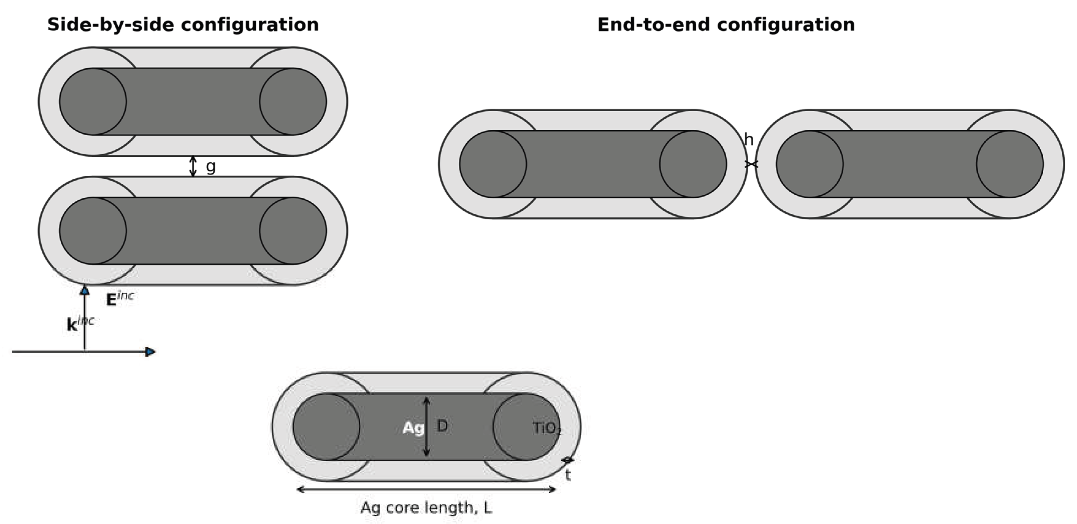
Figure 2.
Locally refined triangular boundary-element mesh for a close core–shell nanorod pair, with concentrated resolution on the opposing gap surfaces.
Figure 2.
Locally refined triangular boundary-element mesh for a close core–shell nanorod pair, with concentrated resolution on the opposing gap surfaces.
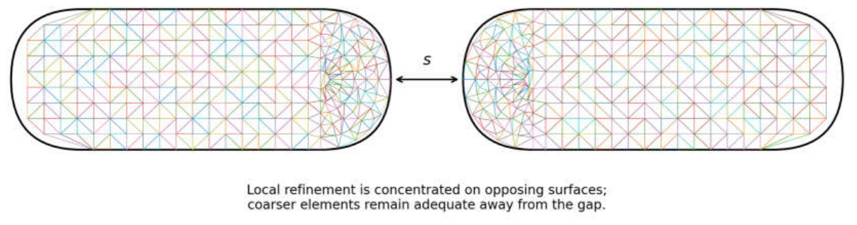
Figure 3.
Region-incidence architecture of the multiregion PMCHWT boundary-integral system for a penetrable Ag–TiO₂ core–shell particle.
Figure 3.
Region-incidence architecture of the multiregion PMCHWT boundary-integral system for a penetrable Ag–TiO₂ core–shell particle.
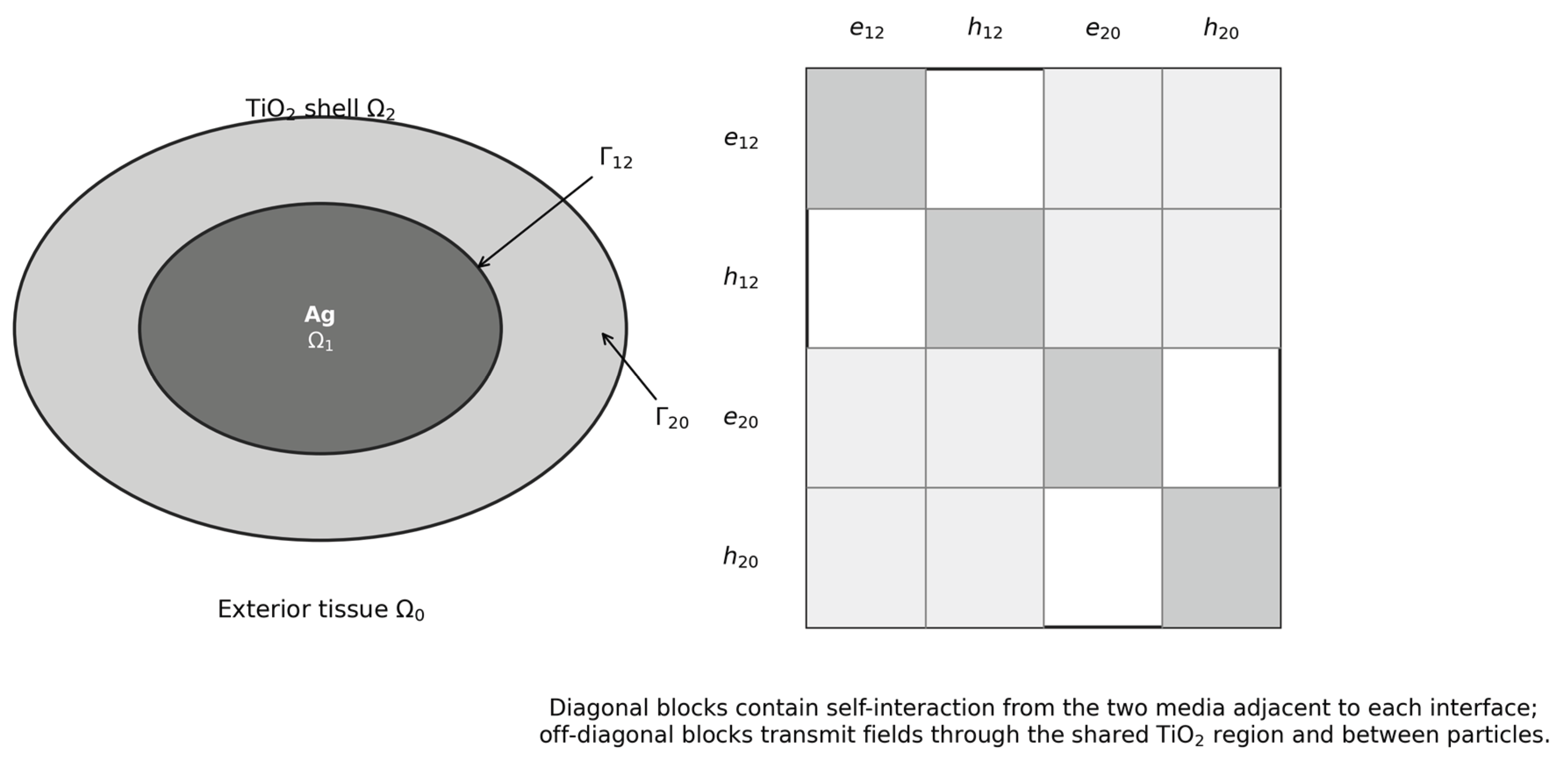
Figure 4.
Prospective two-way electromagnetic–thermal BEM workflow with Picard iteration and audited source transfer.
Figure 4.
Prospective two-way electromagnetic–thermal BEM workflow with Picard iteration and audited source transfer.
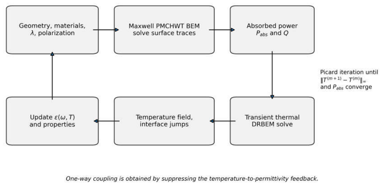
Figure 5.
Reconstruction of side-by-side and end-to-end center distances from the published spacing equations, including the reported optimum configurations.
Figure 5.
Reconstruction of side-by-side and end-to-end center distances from the published spacing equations, including the reported optimum configurations.
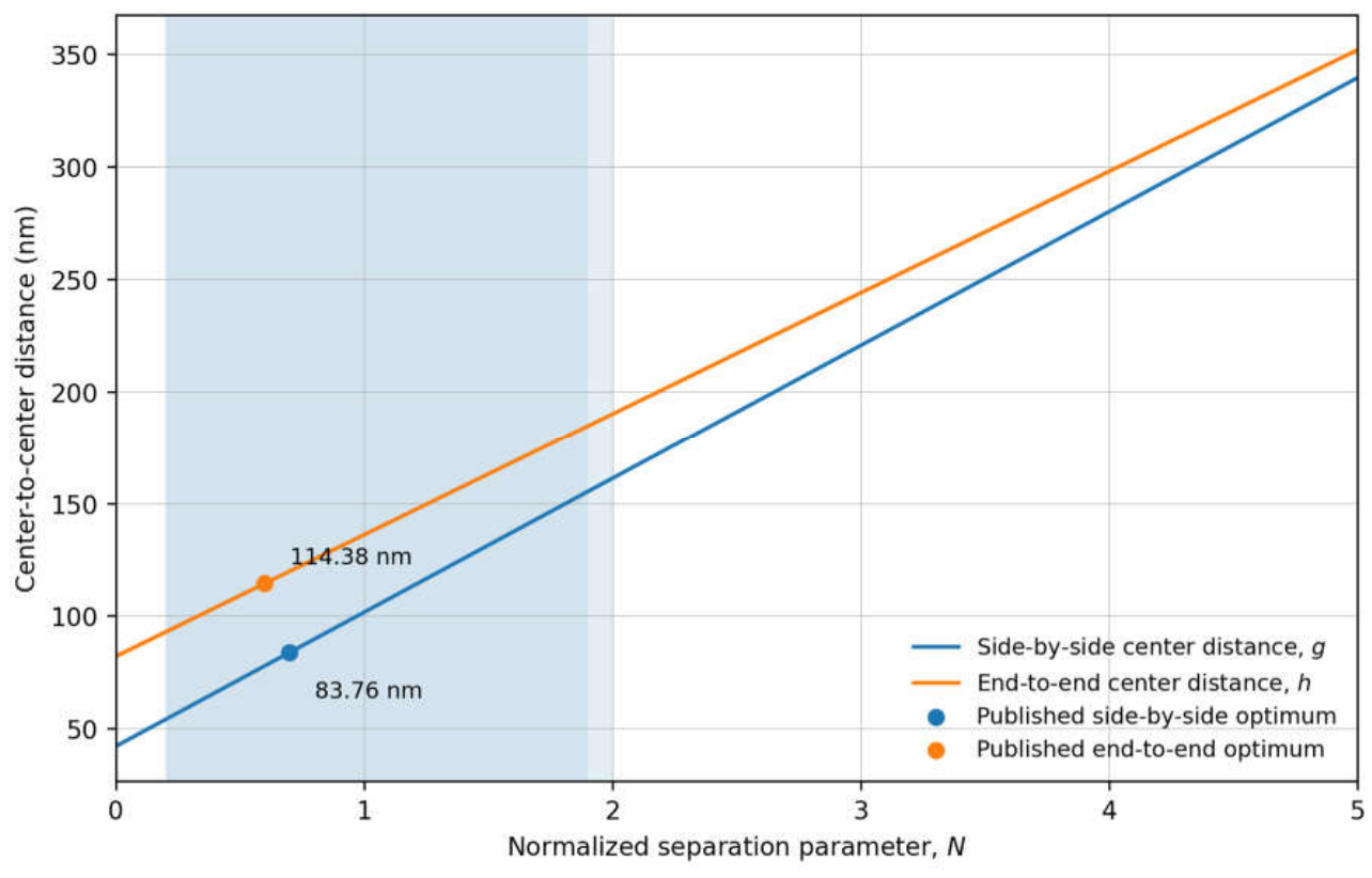
Figure 6.
Convergence of the electrostatic dielectric-sphere BEM polarizability toward the analytical solution under triangular-surface refinement.
Figure 6.
Convergence of the electrostatic dielectric-sphere BEM polarizability toward the analytical solution under triangular-surface refinement.
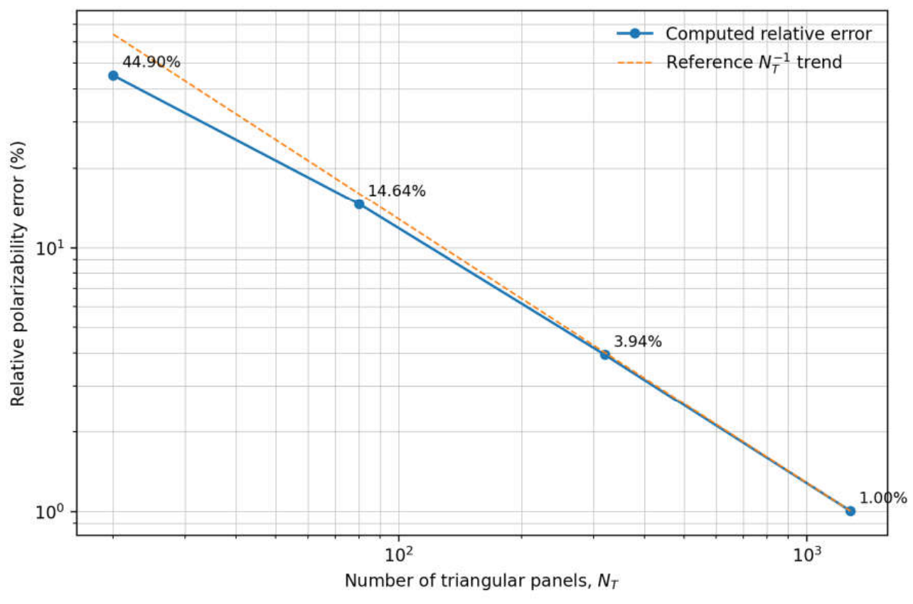
Figure 7.
Analytical transient temperature response around a uniformly heated nanosphere, normalized by the local steady-state temperature rise.
Figure 7.
Analytical transient temperature response around a uniformly heated nanosphere, normalized by the local steady-state temperature rise.
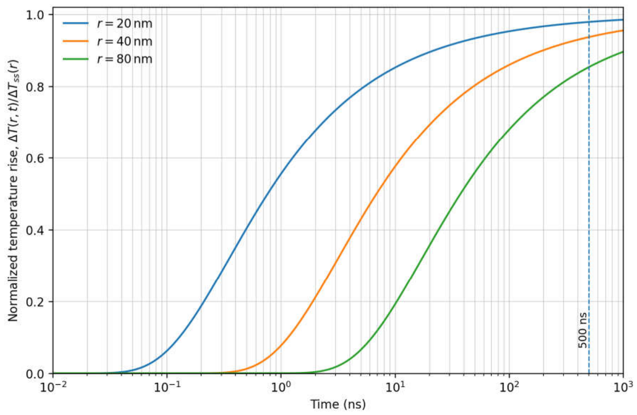
Figure 8.
Equivalent-sphere screening of Ag–TiO₂ and TiO₂–host interface resistance relative to TiO₂-shell conduction resistance.
Figure 8.
Equivalent-sphere screening of Ag–TiO₂ and TiO₂–host interface resistance relative to TiO₂-shell conduction resistance.
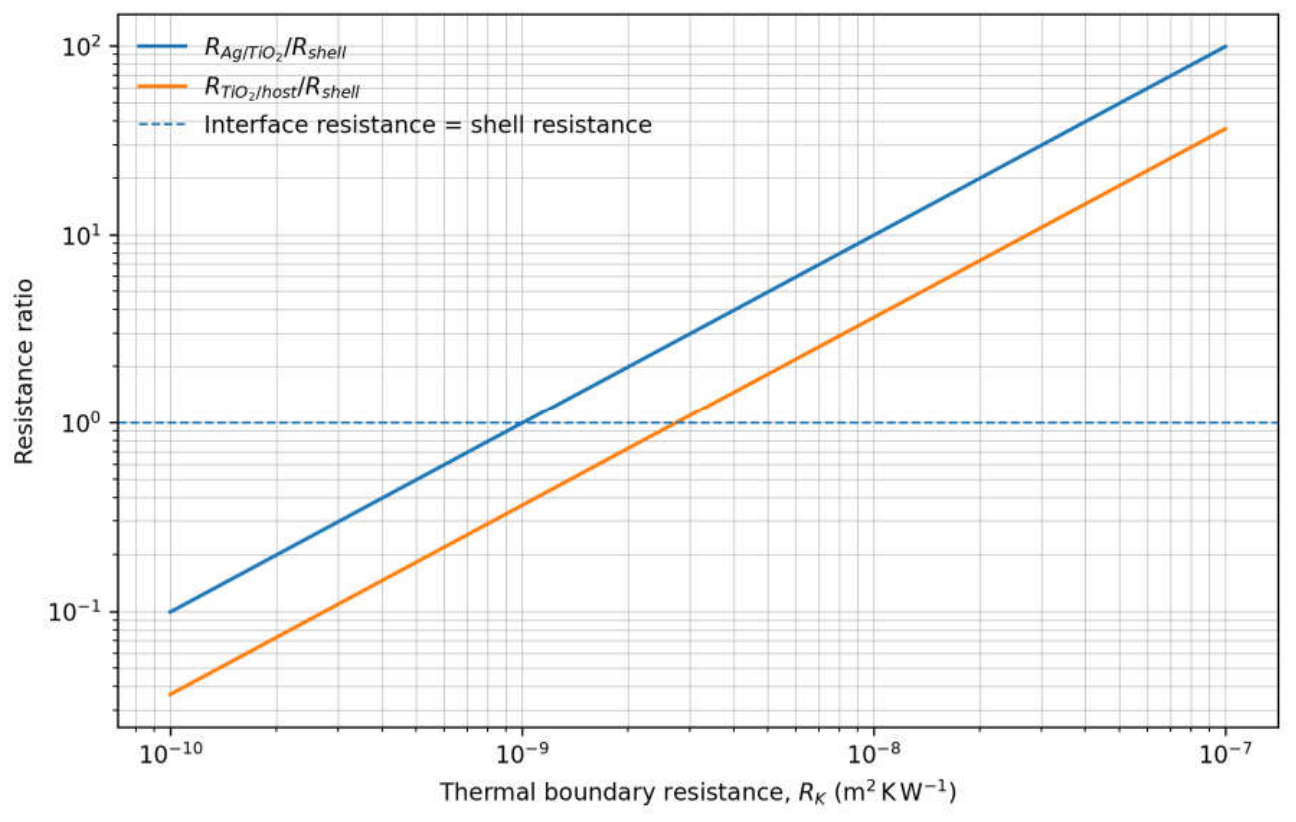
Table 1.
Comparison of domain and boundary methods for coupled thermoplasmonic analysis of core–shell nanoparticle assemblies.
Table 1.
Comparison of domain and boundary methods for coupled thermoplasmonic analysis of core–shell nanoparticle assemblies.
| Criterion | Conventional FEM/FDTD workflow | Electromagnetic surface BEM | Formulated electromagnetic–thermal BEM |
|---|---|---|---|
| Exterior optical domain | Truncated domain with absorbing or radiation boundary | Exact host radiation through the Green function | Exact host radiation through the Green function |
| Exterior thermal domain | Finite host domain with a remote boundary | Not included | Unbounded modified-Helmholtz exterior formulation |
| Discretization | Volume mesh in every region | Surface mesh | Surface mesh for both fields plus limited dual-reciprocity source points |
| Core–shell interfaces | Volume continuity constraints | Multiregion surface traces | Multiregion traces with finite thermal boundary resistance |
| Optical–thermal transfer | Interpolated volumetric loss | Boundary absorption available | Independent boundary/volume power definitions and conservative normalization prescribed; measured residuals not reported here |
| Close particles | Severe volume-mesh demand | Near-singular surface quadrature | Adaptive near-singular quadrature with independent gap refinement |
| Two-way feedback | Possible but costly | Optical update only | Prospective temperature-dependent optical update; not exercised in the reported results |
| Mechanism separation | Commonly inferred from final temperature | Electromagnetic interaction only | Three-calculation mechanism-separation protocol defined; not numerically demonstrated here |
| Primary numerical risk | Artificial-boundary and volume-mesh dependence | Dense matrices and orientation errors | Dense matrices, source transfer, interface jumps, and nonlinear convergence |
Table 2.
Baseline thermophysical properties for reconstruction of the reference Ag–TiO₂ nanorod configuration.
Table 2.
Baseline thermophysical properties for reconstruction of the reference Ag–TiO₂ nanorod configuration.
| Region | Density, ρr (kg m−3) | Heat capacity, cr (J kg−1 K−1) | Conductivity, kr (W m−1 K−1) |
|---|---|---|---|
| Ag core | 10,500 | 235 | 429 |
| TiO2 shell | 3,800 | 686 | 6.7 |
| Host/tissue surrogate | 997 | 4,182 | 0.6 |
Table 3.
Derived geometric, optical, and thermal scales for the reference Ag–TiO₂ nanorod problem.
| Derived quantity | Value | Interpretation |
|---|---|---|
| Ag-core diameter, D | 22.14 nm | Obtained from L/AR |
| Outer particle length, Lo | 82.00 nm | Includes two 10 nm shell layers |
| Outer particle diameter, Do | 42.14 nm | Includes two 10 nm shell layers |
| Ag-core volume, VAg | 2.103 × 10⁻²³ m3 | Spherocylinder volume |
| Host thermal diffusivity, α0 | 1.439 × 10⁻⁷ m2 s−1 | Calculated from k/(ρc) |
| Optical period at 808 nm | 2.695 fs | Establishes optical–thermal scale separation |
| Diffusion length at 500 ns, | 536.48 nm | Exceeds the particle length by a factor of 6.54 |
| Fourier number at 500 ns, | 10.70 | Indicates a near-asymptotic local thermal response |
| Normalized sphere response at r = 40 nm and 500 ns | 0.93697 | Analytical control used in Section 9.4 |
Table 4.
Required verification hierarchy for a complete full-wave electromagnetic–thermal implementation.
Table 4.
Required verification hierarchy for a complete full-wave electromagnetic–thermal implementation.
| Error source | Independent refinement variable | Required observables |
|---|---|---|
| Electromagnetic geometry | surface triangles/RWG unknowns | absorption cross-section, peak wavelength, gap field |
| Near-singular integration | subdivision depth/order | absorbed power, energy residual |
| Thermal boundary mesh | scalar elements/nodes | peak and host temperatures, interface flux |
| DRM source approximation | internal points/RBF choice | integrated source, peak temperature |
| Time integration | constant time step Δt | temperature histories at multiple points |
| Thermo-optic iteration | β and tolerances | converged absorbed power and temperature |
Table 5.
Published finite-element benchmark targets and independent reconstruction of the reference dimer spacing.
Table 5.
Published finite-element benchmark targets and independent reconstruction of the reference dimer spacing.
| Observable | Published value | Independent reconstruction | Use in BEM validation |
|---|---|---|---|
| Ag-sphere FEM/analytical temperature error | below 0.05% | Not recomputed from figure pixels | Thermal benchmark target |
| Approximate local steady time | 500 ns | Analytical response at 40 nm: 93.70% | Time-window check |
| Transverse thermal extent | 339.43 nm | Used in Δg | Side-by-side spacing scale |
| Axial thermal extent | 351.81 nm | Used in Δh | End-to-end spacing scale |
| Side-by-side optimum | N = 0.7, 55.60∘C | Center distance g = 83.76 nm Shell gap 41.62 nm |
Temperature and spacing target |
| End-to-end optimum | N = 0.6, 56.77∘C | Center distance h = 114.38 nm Shell gap 32.38 nm |
Temperature and spacing target |
| Side-by-side treatment interval | 54.03–161.06 nm | 54.03–161.06 nm | Consistent with stated equation |
| End-to-end treatment interval | 93.89–194.97 nm | 92.79–184.53 nm | Formula/text consistency check |
| Absorption reduction as N:5 → 0 | Approximately 5–6 fold | Retained as qualitative target | Spectral validation requirement |
Table 7.
Normalized analytical temperature response around a heated sphere in the reference host.
| Time | r = 20 nm | r = 40 nm | r = 80 nm |
|---|---|---|---|
| 1 ns | 0.55556 | 0.07700 | 0.00004 |
| 10 ns | 0.85213 | 0.57602 | 0.19196 |
| 100 ns | 0.95300 | 0.85964 | 0.67989 |
| 500 ns | 0.97897 | 0.93697 | 0.85360 |
| 1000 ns | 0.98513 | 0.95541 | 0.89619 |
Table 8.
Equivalent-sphere screening of Ag–TiO₂ and TiO₂–host thermal boundary resistances.
| RK (m2 K W−1) | (K W−1) | (K W−1) | ||
|---|---|---|---|---|
| 10−10 | 2.714 × 10⁴ | 0.099 | 9.947 × 10³ | 0.036 |
| 10−9 | 2.714 × 10⁵ | 0.992 | 9.947 × 10⁴ | 0.363 |
| 10−8 | 2.714 × 10⁶ | 9.916 | 9.947 × 10⁵ | 3.634 |
| 10−7 | 2.714 × 10⁷ | 99.158 | 9.947 × 10⁶ | 36.344 |
Disclaimer/Publisher’s Note: The statements, opinions and data contained in all publications are solely those of the individual author(s) and contributor(s) and not of MDPI and/or the editor(s). MDPI and/or the editor(s) disclaim responsibility for any injury to people or property resulting from any ideas, methods, instructions or products referred to in the content. |
© 2026 by the author. Licensee MDPI, Basel, Switzerland. This article is an open access article distributed under the terms and conditions of the Creative Commons Attribution (CC BY) license.
Copyright: This open access article is published under a Creative Commons CC BY 4.0 license, which permit the free download, distribution, and reuse, provided that the author and preprint are cited in any reuse.