

Submitted:
13 November 2026
Posted:
16 November 2026
You are already at the latest version
Abstract
Photovoltaic hosting capacity in low-voltage (LV) networks is usually assessed with balanced or three-wire models, although much of European rural distribution is four-wire with predominantly single-phase connections, where the neutral couples the phases and the voltage response to an injection depends on the phase of the injecting unit. This paper derives that dependence in closed form and builds a coordinated curtailment scheme on it. The test system is a 250 kVA rural substation in north-eastern Romania with 213 supply points, 95.3% of them single-phase, and 53 prosumers, whose feeder, pole and phase are taken from operator records. A four-wire power flow including the EN 50549-1 trip and reconnection sequence compares six inverter strategies with a proposed Trip-Aware Positive-Neighbour Control (PNC), in which the operator releases a per-inverter power ceiling at each averaging window and tightens it only on units with positive voltage sensitivity. The critical-node sensitivity is +3.294 V/kW on the injecting phase and negative on the other two, so only 35 of the 53 units can relieve it, and its sign depends on the power factor. Reactive absorption drives the non-generating phases to 202.0 V at midday. PNC and a local P(U) droop both reach 500 kWp, twice the transformer rating, but PNC curtails 23% less energy and keeps a Jain fairness index of 0.930 against 0.850. Prosumer phase allocation alone is worth 44% of the curtailed energy.
Keywords:
photovoltaic hosting capacity
; four-wire low-voltage network
; signed voltage sensitivity
; single-phase generation
; active power curtailment
; smart inverter control
; protection modelling
; voltage unbalance
; smart meter data
; grid connection rules
1. Introduction
Rooftop photovoltaic (PV) generation has grown faster than the low-voltage networks that host it. In Romania the growth has been particularly abrupt. The prosumer connection rules set out in ANRE Order 228/2018 [1] opened a route for category A generating installations, and rural substations dimensioned for a purely consuming population now carry installed PV capacity comparable to, or larger than, their own transformer rating. The binding constraint in these networks is almost never thermal. It is voltage, and specifically the overvoltage that appears at feeder ends around solar noon, when local demand is at its daily minimum and generation at its maximum.
The hosting capacity literature has converged on a well-tested set of tools for this problem: deterministic, time-series and stochastic assessment of the capacity limit [2,3,4,5,6,7]; reactive power control through a fixed power factor or a Q(U) droop [8,9]; and active power curtailment through a P(U) droop or coordinated set-points [10,11,12,13]. The fairness of curtailment has received sustained attention, because a purely local droop systematically penalises the units electrically farthest from the transformer [13,14,15,16].
Two features of the networks that most need this analysis are, however, routinely simplified away. The first is the neutral conductor. A rural Romanian LV feeder is a four-wire construction, typically twisted aerial bundled cable with a bare or insulated messenger acting as the neutral, whose resistance is comparable to or larger than that of a phase conductor. The second is the connection type: the overwhelming majority of supply points, and therefore of prosumers, are single-phase. Together these mean that an injection does not simply raise "the" voltage. It raises the voltage of the injecting phase by an amount governed by the sum of the phase and neutral path impedances, and it perturbs the other two phases through the neutral return. A three-wire model cannot represent this, and a balanced model cannot even pose the question.
The consequence for control is direct. If the sensitivity of a critical node to a given inverter carries a sign that depends on the phase to which that inverter is connected, then the set of inverters whose curtailment relieves that node is neither "all inverters that observe a high voltage" nor "all inverters upstream of the node". It is a strict subset determined by phase and by the relative magnitudes of the phase and neutral path impedances. Curtailing outside that subset spends energy without buying voltage headroom, and for part of the population it is actively counterproductive.
This paper makes that observation precise on a real network and builds a control strategy on it.
1.1. Novelty and Original Contributions
The six contributions below are labelled N1 to N6 and are referred to by those labels throughout the paper, so that each claim can be traced to the section that establishes it and to the table or figure that quantifies it. Section 2.4 states, against the closest published studies, what is new in each of them.
- N1. Closed-form signed sensitivity. An expression is derived for the sensitivity of the phase-to-neutral voltage magnitude at any node to active power injected at any other node and phase of a four-wire radial feeder, yielding +(R + Rn)/Un on the injecting phase and a negative, asymmetric value on the other two. Existing four-wire studies observe that a single-phase injection perturbs the other phases; none, to the authors’ knowledge, states the sign and magnitude in closed form or uses them.
- N2. Power-factor dependence of that sign, which resolves a contradiction in the literature. Reactive absorption rotates the perturbation, so one non-injecting phase rises instead of falling beyond a threshold power factor, located at cos φ = 0.96 on the test network. Reports that a single-phase injection raises a non-injecting phase and reports that it lowers both are therefore the same expression evaluated at different operating points, not conflicting findings.
- N3. Eligibility set for curtailment. Because the sensitivity carries a phase-dependent sign, only a strict subset of inverters can relieve a given node. Prior curtailment schemes ask how much to curtail and how to share it; this paper asks first which units are eligible at all. On the test network the set contains 35 of 53 prosumers, and the excluded 18 are supporting the critical node rather than stressing it.
- N4. Protection dynamics inside the energy balance. An overvoltage trip under EN 50549-1 is followed by a dead time and a power ramp, so it costs about 1.6 averaging windows of production rather than one. Including this term changes the ranking of the control strategies, and its omission is shown to overstate the performance of every strategy whose compliance is enforced by the protection rather than by the control.
- N5. Trip-Aware Positive-Neighbour Control, together with the implementation condition it requires. The coordinated action must be expressed as a monotone power ceiling constraining the local law; written as a controller acting in parallel with that law it is annulled by it, with no diagnostic. That failure mode is reported here because it is silent and easy to reproduce.
- N6. Undervoltage on the non-generating phases as a binding constraint. Strategies that absorb reactive power to relieve overvoltage are shown to violate the lower EN 50160 limit at midday on a network that shows no undervoltage at all without photovoltaics. Hosting capacity reported from an overvoltage criterion alone therefore overstates the admissible penetration for exactly those strategies.
Two further elements support rather than constitute the novelty. The test system is documented to a level that is uncommon in this literature: feeder, pole, connection type and phase of all 213 supply points and 53 prosumers come from the operator customer database, and Appendix A classifies every model input by origin as documented, measured, catalogue, standard or assumed. And Section 6.5 translates the results into specific amendments to the Romanian connection rules, which is the form in which the findings are intended to reach practice.
The remainder of the paper is organised as follows. Section 2 reviews the state of the art and states the research gap. Section 3 develops the mathematical model, the control laws, the protection model and the proposed scheme. Section 4 describes the case study and its data provenance. Section 5 presents the results, including robustness and tuning studies. Section 6 discusses scope and limitations, and Section 7 concludes.
2. State of the Art and Research Gap
2.1. Hosting Capacity Assessment
Hosting capacity is the maximum distributed generation a network can accommodate without violating an operational criterion. Reviews of the concept and of its quantification methods [2,3,4,17] agree on two points relevant here. First, in LV networks the binding criterion is almost always voltage rather than thermal loading. Second, the reported figures span a very wide range, because they depend strongly on network construction, on the definition of the criterion and on the assumed generation and demand profiles. Comparisons across studies are therefore of limited value; what transfers between networks is the method, not the number.
Methodologically the field divides into deterministic worst-case analysis, time-series analysis, stochastic and Monte Carlo placement, and optimisation-based formulations [3,5,6,18]. Time-series analysis is required whenever the quantity of interest is energy rather than a voltage extreme, and in particular whenever protection dynamics matter, because a trip removes production for longer than the interval that triggered it. Storage, including its use for dynamic voltage regulation and unbalance compensation, and network reconfiguration have been examined as capacity-enhancing measures [19,20,21].
2.2. Four-Wire Modelling and Unbalance
The importance of representing the neutral explicitly in LV analysis is established. Four-wire optimal power flow formulations [22] and unbalance-aware hosting capacity envelopes [23] both start from the observation that neutral current and neutral-point displacement are first-order effects, not corrections. Comprehensive analyses of the voltage unbalance factor in PV-rich non-synthetic LV networks [24] show that unbalance limits can bind before voltage magnitude limits do. The impact of single-phase grid-connected PV on unbalance, losses and voltage, and its dependence on whether the generator is represented as a P-Q or a P-V source, is analysed in [25]. Work on phase load balancing using smart-meter data [26,27,28], and on the smart metering systems that supply such data [29], has established that per-phase allocation of single-phase customers is both knowable from operator records and consequential for losses and voltage quality; the same records make the present study possible.
Closest to the present work, Eliáš et al. [30] model a Slovak LV network with an explicitly non-ideal PEN conductor and compare scenarios with single-phase and three-phase PV. They report that connecting single-phase PV to one phase drives voltage unbalance beyond the EN 50160 [31] limit at every node, that the PEN conductor can be overloaded, and that for the same network impact a three-phase connection admits roughly five times the power of a single-phase one. They also report a phenomenon of direct relevance here: a single-phase injection on one phase changes the phase-to-PEN voltage on the other phases, which they explain through the potential acquired by the PEN conductor. Their study is deterministic and worst-case, the network is synthetic and regular, and the measures proposed are explicitly passive, "fit and forget" ones: conductor cross-section, symmetrisation of connections, limitation of installed power, fixed power factor. Their concluding section identifies as future work exactly the two steps taken here, namely a model replicating a real network with real supply-point placement and phase allocation, and the testing of active management strategies on it.
2.3. Inverter Control and Curtailment
Local voltage-dependent inverter control is standardised in EN 50549-1 [32] and analysed in depth in [33], which remains the reference treatment of Q(U) and P(U) parameterisation in LV networks. Reviews of voltage optimisation in PV-rich networks [34] catalogue the available levers, and recent work extends them to learning-based Volt-Var control aimed at unbalance at the point of common coupling [35] and to loss reduction and voltage profile enhancement in radial networks dominated by distributed generation [36]. Reactive control is attractive because it does not destroy energy, but its effectiveness is bounded by the X/R ratio of LV feeders and, as shown in Section 5.4, by the apparent power headroom the inverter retains at solar noon.
Active power curtailment is the reliable lever, and the literature on it is largely a literature about fairness. Adaptive real power capping [13], decentralised strategies that improve fairness without communication [14], fair coordination of distributed energy resources with Volt-Var control [15] and rule-based centralised schemes computing equitable curtailment factors [16] all address the same asymmetry: a local droop curtails the electrically remote units first and hardest. Several of these works compute a voltage sensitivity matrix, and some do so for unbalanced three-phase networks. What they do not do is treat the sign of that sensitivity as the object of interest, or use it to exclude inverters from the curtailment set. The prevailing formulation asks how much to curtail and how to share it; the formulation proposed here asks first which units are even eligible.
2.4. Research Gap
Table 1 positions the present approach against the closest studies. Three gaps are addressed. The first is representational: hosting capacity studies that model the neutral explicitly rarely also use documented per-supply-point phase allocation, and studies that use real operator data rarely model the neutral. The second is analytical: the signed, phase-dependent sensitivity of a four-wire feeder is available in closed form but has not been used to define an eligibility set for curtailment. The third is procedural: coordinated schemes are usually formulated as controllers, and the failure mode in which a coordinator competing with a local droop is annulled by it has not, to the authors’ knowledge, been reported.
3. Mathematical Model
3.1. Four-Wire Radial Network
The network is a radial tree of N nodes rooted at the 0.4 kV busbar of the MV/LV transformer. Each branch k carries three phase conductors of series impedance Zph,k and a neutral conductor of series impedance Zn,k. Shunt admittances are neglected, which is standard at LV where line lengths are short, and cable charging is negligible against load current. The neutral is bonded to earth at the transformer only; repeated earthing at poles, which exists in practice, is omitted, and this omission is conservative because it maximizes neutral-point displacement.
Let Ip,k denote the current flowing from the parent node to the child node of branch k in phase p, with the load convention. The neutral carries the return of the three phase currents,
so that the potential of the neutral conductor at the child node differs from that at the parent node. Writing potentials of the phase and neutral conductors separately and subtracting gives the phase-to-neutral voltage at the child node,
The second term is the mechanism that the present paper turns into a control law. It vanishes only when the three phase currents sum to zero, that is, only under balanced operation. Any single-phase injection makes it non-zero and therefore perturbs all three phases, not only the injecting one.
3.2. Common-Path Impedance Formulation
Because the network is radial, the branch currents are determined by the node injections through the path incidence matrix. Let Π ∈ {0,1}^(N×M) have Πik = 1 when branch k lies on the path from the busbar to node i. Then the current in branch k is the sum of the injections downstream of it, and substituting into (2) and summing along the path gives a closed-form expression for all node voltages at once:
where U and I are N×3 complex matrices of phase-to-neutral voltages and injected currents, 1₃ is a column of ones, and the common-path impedance matrices are
Entry (i, j) of Zph is the sum of phase impedances over the branches common to the paths from the busbar to nodes i and j, and analogously for Zn. The transformer short-circuit impedance ZT is added to every entry because the whole network current passes through it; ZT0 is the corresponding zero-sequence path, taken equal to ZT for the Dyn11 connection.
This formulation has three practical advantages over a branch-by-branch backward/forward sweep. The matrices are assembled once, so each iteration of the nonlinear solution is a single matrix product; the sensitivity expressions of Section 3.4 can be read directly off the matrix entries; and the phase and neutral contributions remain separated throughout, which is what makes the sign structure visible.
3.3. Nonlinear Solution
The nonlinearity enters only through the constant-power injection model, I = conj(S ⊘ U), where S is the N×3 matrix of complex powers with the load convention. The system is solved by damped fixed-point iteration,
with λ = 0.85 and a convergence tolerance of 10⁻⁸ V on the maximum voltage update. Typical convergence is reached in 12 to 18 iterations from a flat start and in fewer than 8 when warm-started from the previous time step. On the 84-node test system one power flow evaluation costs 0.95 ms.
A second fixed point is nested inside the first whenever a voltage-dependent inverter law is active, because the inverter set-points depend on voltages that depend on the set-points. Steep droops make this loop ill-conditioned: a P(U) characteristic that falls from full output to zero over 5 V has a large gain, and a constant-step iteration enters a limit cycle. An adaptive step is therefore used, halving λ whenever the residual increases, which restores monotone convergence in all cases reported. Convergence of every reported case was verified explicitly and the power balance closes to better than 0.1 W once transformer copper losses are included.
3.4. Signed Voltage Sensitivity
Let node nc on phase pc be the critical node, and let inverter i be connected at node j on phase p. At unity power factor the injection current is I = −(P/Un)e(jθp), where θp is the phase angle of the corresponding source phasor. Substituting into (3), projecting the resulting voltage perturbation onto the direction of the critical phasor and dividing by the injected power gives
where δ is the Kronecker delta. Two cases follow. On the injecting phase the rotation is unity and
with R and Rn the real parts of the common-path phase and neutral impedances. On the two remaining phases the rotation is ±120° and
Three properties of (8) matter for control. It is negative, so an inverter on a non-critical phase supports the critical node rather than stressing it. It is asymmetric between the two remaining phases, the asymmetry being carried entirely by the neutral reactance and vanishing only if Xn = 0. And it is governed by the neutral, not the phase, impedance: the coupling exists only because the return path has resistance.
The set of inverters that can relieve a given critical node by reducing output is therefore the set with positive sensitivity. We call its members the positive neighbours of that node. Membership is decided by phase, not by proximity: an inverter close to the critical node but on another phase is excluded, while a distant inverter on the same phase is included with a weight proportional to the impedance its path shares with the critical node.
3.5. Dependence on the Injection Power Factor
Equations (7) and (8) assume unity power factor. When the inverter absorbs reactive power, as under a fixed power factor or a Q(U) droop, the injection current rotates by the power factor angle φ and its magnitude scales by 1/cos φ. Writing the injected complex power as P(1 − j tan φ), the injected current becomes (P/Un)(1 + j tan φ) e(jθp), and repeating the projection gives, for a non-injecting phase at rotation Δ = θp − θpc = ±120°,
The bracket contains a term proportional to tan φ whose sign differs between the two non-injecting phases. Reactive absorption therefore deepens the depression on one of them and lifts the other, and beyond a threshold power factor the lifted phase changes sign and rises. This is not a curiosity. It explains why four-wire studies that assume unity power factor report both non-injecting phases falling, while studies that assume an absorbing power factor, such as the cos φ = 0.97 of [30], report one of them rising.
3.6. Local Inverter Control Laws
Five local laws are implemented, together with a no-PV reference case and two fleet-level cases. They are summarised in Table 2. The apparent power envelope is enforced with active power priority, which is the default behaviour in EN 50549-1: the active set-point is kept and the reactive set-point is limited to the remaining headroom,
This is not a modelling detail. Enforcing the envelope by proportional scaling of both components instead would silently curtail active power and misattribute the resulting voltage relief to the reactive control, an artefact discussed in other section.
3.7. Protection and Reconnection
The protection model follows EN 50549-1 [32] and the Romanian technical norm approved by ANRE Order 228/2018 [1]. Two overvoltage stages are implemented. Stage U> operates at 1.10 Un = 253 V on the ten-minute mean value, and stage U>> at 1.15 Un = 264.5 V instantaneously. Reconnection after a trip requires a dead time of 60 s, a voltage inside the band, and then a power ramp limited to 10% of rated power per minute.
Since the metering data are 15-minute averages, the simulation step is used as the averaging window of stage U>. A longer window smooths short excursions, so relative to the ten-minute window of the standard it tends to under-count trips, and in this respect the trip-related losses reported below are a lower bound. A trip detected in step t removes the unit for the whole of step t+1 and, through the dead time and the ramp, for part of step t+2. The production lost per trip is
With a dead time tdead = 60 s, a ramp from zero to rated power of tramp = 600 s and Δt equal to the ten-minute window of the standard, (11) gives 1.6 windows, and this value is applied to every trip in the simulation. Evaluated on a 15-minute step the same sequence would cost 1.4 steps, so the trip loss of the strategies that trip is overstated by at most 0.2 step per trip; S4 and S7 never trip and are unaffected. This term is not cosmetic. Without it, strategies that permit frequent tripping appear to deliver more energy than they do, and the ranking of the reactive strategies against the active ones inverts. Reporting a hosting capacity from voltage extremes alone, with the inverters modelled as never disconnecting, therefore overstates the performance of any strategy that relies on the protection to enforce the limit.
3.8. Trip-Aware Positive-Neighbour Control
PNC is a coordinated scheme that acts between measurement windows and requires only that the operator can send a power ceiling to each inverter and knows the network topology and phase allocation. It does not require real-time telemetry from the inverters. The procedure for one window is as follows.
- Step 1. Release. Every ceiling is set to the inverter rating, Pmax,i = Sn,i. Releasing rather than carrying over the previous window prevents the ceilings from ratcheting down over the day and is what makes the scheme recover automatically when irradiance falls.
- Step 2. Solve. The network is solved with the local laws active and the ceilings applied as upper bounds, using the nested fixed point of Section 3.3.
- Step 3. Identify. The critical node and phase (nc, pc) are taken as the argument of the maximum phase-to-neutral voltage magnitude over all nodes and phases.
- Step 4. Select. The signed sensitivity si of every inverter to that node is evaluated from (6). The active set A contains the inverters with si > 0.15 max(s) that are still producing. Inverters with negative sensitivity are excluded; curtailing them would not help.
- Step 5. Allocate. The required reduction is distributed over A with a fairness weight.
- Step 6. Tighten. Ceilings are lowered, never raised, within the window. Steps 2 to 6 repeat until the target voltage is met or a maximum of twenty passes is reached.
The allocation in Step 5 is
with the fairness weight
where Ecurt,i is the energy already curtailed from unit i on the day and Ēcurt its mean over the active set. The weight discounts units that have already borne curtailment, so that the burden rotates across the fleet within the positive-neighbour set. The factor κ = 1.15 slightly overshoots the linear estimate, which accelerates convergence of the outer loop without risk because the ceilings are subsequently re-evaluated. The target is Utarget = 251 V, one volt of margin below the 253 V limit. Allocation (12) is not a heuristic. For κ = 1 it is the solution of the weighted least-norm problem of minimising Σ ΔPi²/wi over i ∈ A subject to Σsi ΔPi = Ucrit − Utarget, that is, the smallest weighted curtailment that removes the excess voltage at the critical node to first order. Units with larger sensitivity therefore carry proportionally more of the reduction, and units that have already been curtailed carry less, through wi. The ceilings are then re-evaluated by the full power flow in Step 2, so the linearization error of (6) does not accumulate across passes.
One implementation detail determines whether the scheme works at all. PNC was first implemented as a controller acting in parallel with the local droop inside the nested fixed point, that is, as an additional input to the set-point calculation. In that form it has no effect whatsoever: the local law restores the output that the coordinator has just removed, and the fixed point converges to the uncoordinated solution. Only when the coordinated action is expressed as a constraint on the local law, a monotone ceiling that the local law may respect but not exceed, does the scheme act. This failure is silent, in the sense that the simulation converges and reports plausible voltages and energies, and it is recorded here because it is easy to reproduce.
3.9. Performance Metrics
Five metrics are reported. The first two are compliance counts against EN 50160: the number of averaging windows in which any node exceeds 253 V, and the number in which any node falls below 207 V. The third is the number of unit-trips over the day. The fourth is the unavailable photovoltaic energy,
which aggregates deliberate curtailment and production lost to trip and reconnect cycling, and is also reported as a percentage of the potential. The fifth is the Jain index of the per-unit ratio of delivered to available energy,
Defining fairness on the delivered fraction rather than on the curtailed energy is deliberate: it is the quantity the prosumer experiences, and it does not reward a strategy for curtailing everyone equally badly. Hosting capacity is defined as the largest installed capacity at which no window exceeds 253 V and no unit trips, which is stricter than voltage compliance alone.
4. Case Study: A Rural Low-Voltage Substation
4.1. The Network
The study substation, designated here S-NE for anonymity, is a pole-mounted 20/0.4 kV unit in a village of the north-eastern region of Romania. It belongs to the distribution system operator of that region and lies inside the area of an ongoing operator pilot programme on flexibility services. The transformer is rated 250 kVA with uk = 4%, resolved into uR = 1.30% and uX = 3.78%, which gives a per-phase short-circuit impedance of 8.25 + j24.00 mΩ referred to the low-voltage side. The substation supplies four feeders totalling 83 poles. Figure 1 shows the single-line diagram of the network: the poles are numbered by feeder, and each pole that carries supply points is marked as serving consumers only (C) or at least one prosumer (PV).
Feeder 1 runs from a cable head, then branches after pole 3 into two overhead laterals of 12 and 10 poles. Feeder 2 is the dominant feeder in both extent and customer count: it reaches 0.750 km of electrical distance and terminates in a sectionalizing cabinet, and its far end is the critical node in every case examined below. Feeders 3 and 4 are short. Table 3 summarizes the network data and Table 4 the conductor parameters.
4.2. Data Provenance
A recurring difficulty in LV hosting capacity studies is that the inputs which most affect the result, namely phase allocation and the spatial distribution of prosumers, are the ones most often assumed. Here they are documented. The operator customer database provides, for every supply point, the feeder, the pole, the connection type and the phase; it also identifies which supply points hold a photovoltaic installation. Table A1 in Appendix A classifies every model input by origin as documented, measured, catalogue, standard or assumed, so that a reader can see which conclusions rest on which class.
Two quantities remain assumptions. Span lengths are not recorded and are taken as 35 m for overhead spans and 50 m for cable sections, values typical of Romanian rural construction. The internal branching of Feeder 2 is inferred from the six repeated feeder labels on the single-line diagram and modelled as a trunk of 15 poles with six laterals; the pole numbering in the customer database runs from 2 to 46, which matches the 45 poles shown on the diagram, and the model adds pole 1, which carries no supply point, at the end of the cable head, giving the 46 nodes of Feeder 2 in Table 3. Section 5.7 quantifies the effect of both assumptions. One correction arising from the operator data deserves mention because it inverts a natural reading of the single-line diagram. The diagram lists connection counts per feeder without unambiguous association, and the obvious pairing attributes the largest group to Feeder 1. The customer database shows the opposite: Feeder 2 carries 130 supply points against 71 on Feeder 1. This is also the physically coherent reading, since Feeder 2 has 46 poles against 25. A hosting capacity computed on the reversed assignment would place the stress on the wrong feeder.
4.3. Measured Profiles
Demand and generation profiles were derived from 15-minute metering and are shown in Figure 2. The demand profile is the aggregate of 242 metered supply points over a summer week, divided by the number of points, so that it carries the real diversity of the population rather than the shape of an individual household. Its peak-to-mean ratio is 3.66, and the mean-day peak is 422 W per supply point. This is cross-checked against five individual annual load curves at 15-minute resolution, which give a summer mean of 265 W per point, consistent with the 228 W obtained from the aggregate.
The generation profile is the net export of two metered prosumers on the most productive day of the record, cleaned of meter register artefacts at the 99.5th percentile. Using net export rather than gross production is deliberate: what the network sees at the connection point, and what the protection function measures, is the net injection. The two units export 4829 and 4835 kWh over 2025, and 29.3 kWh on a clear summer day, with a peak net export of 3.92 kW, consistent with the 5 kWp single-phase installations typical of the Romanian residential prosumer segment.
The measured busbar voltages, 234.45, 234.67 and 235.69 V on the three phases, both confirm the assumed +2.5% transformer tap and provide the slack condition. The measured voltage unbalance factor at the busbar ranges from 0.07% to 0.59%, well within the 2% limit, which is expected: unbalance grows along the feeder, and the busbar is where it is smallest.
4.4. Simulation Setup
The reference case is the documented fleet: 53 prosumers at their recorded poles and phases, with a measured peak net injection of 207.9 kW against a demand peak of 98.3 kW on the same day, that is, a generation-to-demand peak ratio of 2.1. The penetration sweep scales the installed capacity from 100 to 500 kWp, twice the transformer rating, holding the prosumer locations and phases at their documented values so that only the magnitude changes. All computations were carried out in GNU Octave 8.4.0 [37] without additional toolboxes, on a single core.
5. Results
5.1. Validation of the Signed Sensitivity
At the end of Feeder 2, which is the critical node throughout, the common-path phase resistance is R = 0.307 Ω and the neutral path resistance is Rn = 0.450 Ω, so the return path contributes more than the outgoing one. The neutral reactance is Xn = 0.0839 Ω and the X/R ratio of the single-phase loop, 2Xn/(R + Rn), is 0.222.
Equations (7) and (8) give +3.294 V/kW on the injecting phase and −1.295 and −0.663 V/kW on the other two. A full power flow with 5 kW injected at that node on phase L1 returns +16.08, −6.41 and −2.90 V, that is +3.22, −1.28 and −0.58 V/kW. Both the magnitude and the asymmetry are reproduced; the residual difference is the second-order term neglected in the linearization.
The same 5 kW injected in balance produces +2.25, +2.32 and +2.27 V. The ratio of the worst single-phase rise to the balanced rise is therefore 6.9. This factor is the quantitative reason why a balanced model cannot be used to set hosting capacity on a network with 95.3% single-phase connections, and it is consistent with the roughly fivefold ratio reported in [30] for a different four-wire network with a different conductor mix.
Table 5 varies the injection power factor and confirms the prediction of Section 3.5. At unity power factor both non-injecting phases fall. As reactive absorption increases, the depression on L2 deepens while that on L3 shrinks, crosses zero near cos φ = 0.96, and becomes a rise. At cos φ = 0.85 phase L3 rises by 3.30 V while phase L2 falls by 11.19 V. Reports that a single-phase injection raises a non-injecting phase and reports that it lowers both are therefore not in conflict; they are the same expression evaluated at different power factors.
Figure 3 shows the consequence for control. Of the 53 documented prosumers, 35 have positive sensitivity to the critical node and 18 have negative sensitivity. The spread within the positive set is a factor of about twenty, from 2.66 V/kW down to a few hundredths, so even inside the eligible set a uniform allocation would be inefficient. The 18 units with negative sensitivity are supporting the critical node; curtailing them raises it.
5.2. Reference Case
Table 6 gives the outcome of the reference case (53 documented prosumers, 207.9 kW peak net injection, one clear summer day at 15-minute resolution) for all eight strategies. Without photovoltaics the network is comfortable: the maximum voltage is 234.28 V and the minimum is 211.46 V at the evening demand peak, with no violation of either limit. Counts are over the whole day and the whole network. Unavailable energy includes curtailment and production lost to trip and reconnect cycling; the percentage is of the potential 1555.3 kWh.
Uncontrolled operation is not viable. Strategy S1 exceeds the upper limit in 26 of the 96 windows and produces 308 unit-trips, losing 27.1% of the available energy without any deliberate curtailment at all. That loss is entirely the protection function doing its job, and it is invisible to a study that does not model tripping. Figure 4 shows the characteristic sawtooth: a set of inverters disconnects on the ten-minute stage, waits out the dead time, ramps back, and crosses the threshold again.
The two strategies that curtail active power in response to voltage, S4 and S7, both hold the network below 253 V for the entire day with no trips. They differ in cost. The local P(U) droop forgoes 141.4 kWh, the coordinated scheme 108.9 kWh, a reduction of 23%. PNC also achieves a higher Jain index, 0.987 against 0.972, so the saving is not obtained by concentrating curtailment on a few sites. The mechanism is the one identified in Section 5.1: the local droop curtails every unit that observes a high local voltage, whereas PNC curtails only those that actually move the critical node, and among them in proportion to how much they move it.
5.3. Simultaneous Over- and Undervoltage
Column five of Table 6 records a constraint that hosting capacity studies rarely evaluate. Without photovoltaics the network never approaches the lower EN 50160 limit: the minimum phase voltage is 211.46 V and it occurs at the evening demand peak. With single-phase generation the picture changes. Strategy S1 drives the minimum to 206.61 V in two windows. The strategies that absorb reactive power are markedly worse: S2 reaches 203.84 V in six windows and S5 reaches 202.04 V in seven. These minima occur around midday, not in the evening.
The mechanism is exactly the one derived in Section 3.4 and Section 3.5. A single-phase injection depresses at least one non-injecting phase through the neutral, and reactive absorption deepens that depression, as the L2 column of Table 5 shows. The strategies designed to relieve overvoltage therefore create a violation of the opposite constraint. Figure 5 shows the three phase voltages at the critical node under S1, with both limits marked: the phases separate by more than 60 V at midday, and the lower envelope approaches 207 V in the same windows in which the upper envelope exceeds 253 V.
The practical consequence is that a strategy evaluated against overvoltage alone can be judged successful while creating a violation it never measures. On a network with 95.3% single-phase connections the undervoltage criterion is not a formality, and it binds first for precisely the reactive strategies that are usually recommended as the least intrusive remedy for overvoltage.
5.4. Reactive Power Headroom Limits Q(U)
The effectiveness of Q(U) on this network is governed by inverter sizing rather than by the X/R ratio, which is the explanation usually offered. At solar noon the inverter is at rated active output, so the reactive power it can supply is whatever the apparent power envelope leaves. Table 7 varies the ratio Sn/Pn with everything else fixed.
This is not an artefact of the present model. Cantero Gubert et al. [9] report the same mechanism from laboratory measurements on a physical PV inverter: because active power is prioritised, reactive power availability collapses at high generation, and the voltage then rises both from the active injection and from the loss of reactive support. What the present study adds is the quantification of that effect on the delivered energy of a whole feeder over a day. At Sn = Pn the inverter has no reactive headroom at exactly the hour when the network needs it, and Q(U) is close to inoperative. Even at Sn = 1.2 Pn it leaves 98 trips and does not bring the network into compliance. The non-monotone maximum voltage is itself informative: when protection dynamics are modelled, the voltage extreme is a poor figure of merit, because it is determined by where in the cycle the sampling falls. Energy is the robust metric.
This result also carries a warning about model construction. If the apparent power envelope is enforced by scaling both components proportionally rather than by giving active power priority, the reactive law silently curtails active power, and the voltage relief that follows is attributed to Q(U). In an earlier version of this model that formulation produced an apparent 34 V of relief from Q(U) alone, an artefact that disappeared once (10) was enforced.
5.5. Hosting Capacity and Delivered Energy
Table 8 gives the maximum network voltage across the penetration sweep and the resulting hosting capacity under the strict criterion of Section 3.9.
Figure 6 summarises the hosting capacity of each strategy. Two strategies reach 500 kWp, the local P(U) droop and PNC, and Table 9 gives the delivered energy of the three strategies that curtail active power.
Since both compliant strategies reach the same capacity, the separation between them appears in delivered energy rather than in feasibility, as Figure 7 shows.
PNC delivers more energy at every penetration level, with the advantage peaking near 350 kWp and remaining around 4% at the top of the sweep. In absolute terms the gain is 94 kWh/day at 500 kWp, roughly 34 MWh/year if summer conditions are taken as representative of the binding period. The margin grows with penetration in the mid range because the number of units whose curtailment is wasted under a purely local droop grows with the size of the fleet.
The heterogeneous fleet is the most instructive negative result in the table. Its hosting capacity is 100 kWp, the same as the fixed power factor fleets S2 and S5 and lower than either voltage-dependent local law. A population in which 40% of inverters operate at unity power factor cannot be rescued by the remaining 60%, because the units without a voltage-dependent law continue to inject at exactly the moment the network needs them not to. The cost of an unharmonised inverter population is therefore not a marginal degradation but a collapse to the behaviour of its least capable members. Since PNC is applied on top of the same heterogeneous fleet, its recovery from 100 to 500 kWp also measures what an operator-side ceiling can buy when the fleet cannot be replaced.
5.6. Fairness and Network Losses
Table 10 reports the Jain index and the network losses across the sweep. The fairness of the local droop degrades steadily with penetration, from 0.999 at 100 kWp to 0.850 at 500 kWp, which is the well-documented locational bias: the units at the end of Feeder 2 see the highest voltage and are curtailed first and hardest. PNC holds 0.930 at the same level, because the fairness weight of (13) rotates the burden within the positive-neighbour set.
The loss columns require a careful reading and are reported because they are easy to misinterpret. PNC has higher losses than the local droop at high penetration, 170.0 against 119.6 kWh/day at 500 kWp. This is not an inefficiency: PNC delivers 94 kWh/day more energy, and that energy has to flow. The heterogeneous fleet, which delivers least, has the highest losses of all, 249.8 kWh/day, because its energy flows in an unbalanced pattern with large neutral currents. Loss per unit of delivered energy is 4.9% for S4, 6.7% for S7 and 12.1% for S6, so on that normalized measure the ranking is the expected one and the heterogeneous fleet is the clear outlier.
5.7. Robustness to the Two Assumptions
Span lengths and the internal structure of Feeder 2 are the only assumed quantities that affect the electrical model. Table 11 varies the span length by ±30% around the assumed 35 m, which brackets any plausible construction, and Figure 8 shows the result.
The absolute voltages carry the length uncertainty, as expected, since voltage rise is close to linear in length. The comparison between strategies does not. Both controlled strategies remain compliant across the whole range, PNC holds its target exactly, and the curtailed energy scales smoothly. In other words, the assumption affects how much energy the operator must give up, which a survey would refine, but not which strategy is preferable, which is the object of the study.
Table 12 and Figure 9 address the more consequential input, the phase allocation of the prosumers. Three cases are compared: the documented allocation (13/21/19), a perfectly balanced one (18/18/17), and a concentrated one in which all single-phase prosumers sit on the same phase. The three-phase prosumers are left unchanged in all cases.
The effect is large and asymmetric. Moving from the documented allocation to a balanced one reduces the curtailed energy by 44% under the local droop and 35% under PNC, at no cost. Moving to a concentrated allocation multiplies it by 6.6 and drives the minimum voltage to 183.2 V, far outside any admissible band, which no inverter-side control can repair because the constraint is then undervoltage on the phases that have no generation to curtail.
The operational reading is that phase allocation of prosumers is a hosting capacity parameter of the same order as conductor cross-section, and it is essentially free to manage. Operators already record the phase at connection, as the database underlying this study demonstrates. Using that field as a constraint when approving new prosumer connections, rather than as a passive record, is the cheapest capacity measure available and it requires no equipment at all. This complements the recommendation of [30] to prefer three-phase connections where feasible: where single-phase connection is unavoidable, the phase should be chosen rather than defaulted.
5.8. Tuning the PNC Target
PNC has one operational parameter, the target voltage Utarget. Figure 10 sweeps it from 249 to 252.5 V at 250 kWp. The trade-off is close to linear: each additional volt of margin below the 253 V limit costs about 17 kWh/day of photovoltaic energy, and every setting in the range produces zero violations and zero trips. The achieved maximum voltage tracks the target to within 0.01 V, which confirms that the outer loop converges.
The value chosen for the rest of the study, 251 V, is deliberately conservative. An operator confident in the accuracy of its network model and its measurement chain could move to 252.5 V and recover a further 20 kWh/day, roughly 11% of the curtailed energy at that penetration. The right setting is a function of model confidence rather than of the control scheme, which is an argument for stating it explicitly as a parameter rather than burying it in a droop characteristic.
5.9. Computational Performance
One four-wire power flow evaluation on the 84-node system costs 0.95 ms. A full day at 15-minute resolution costs 0.17 s for the uncontrolled case, 2.30 s for the local P(U) droop and 10.89 s for PNC, the difference being the nested and outer iterations. The whole study reported here, comprising the reference case, the oversizing study, the penetration sweep for seven strategies and the three robustness studies, runs in under 25 minutes on a single core. This matters for the practical claim. PNC as formulated requires, per window, one sensitivity evaluation from a matrix the operator can precompute once from its network model, and a small number of power flow solutions. Nothing in the scheme requires an optimization solver, and the sensitivity expression (6) is a lookup of two matrix entries and a rotation. A ceiling computed centrally and broadcast every fifteen minutes is well within the capability of the metering and communication infrastructure that a programmed such as the operator pilot is already deploying.
6. Discussion
The central claim of this paper is that on a four-wire network with predominantly single-phase connections, the identity of the inverters that should be curtailed is a property of the phase topology and is computable in closed form. Four consequences follow for practice, taken in turn below, after which Section 6.5 states what they imply for the Romanian connection rules and Section 6.6 the limits of the study.
6.1. Phase Allocation as a Planning Variable
Phase allocation is a planning and operating variable, not a bookkeeping detail. On S-NE the supply points are close to balanced across phases, 66/71/66, but the prosumers are not: 13, 21 and 19. Because the sensitivity is phase-specific, a fleet concentrated on one phase concentrates its stress on that phase and cannot be relieved by units on the others. Table 12 quantifies what this is worth: the difference between the documented and a balanced allocation is 44% of the curtailed energy. This connects directly to the phase load balancing literature [26,27,28], which has developed algorithms for reallocating single-phase customers using smart meter data; the present result suggests those algorithms should weight prosumers differently from pure consumers, because a prosumer contributes to the constraint in both directions.
6.2. Two Constraints, Active at the Same Time
The two voltage constraints are simultaneous, and the strategies usually recommended for one of them worsen the other. A control strategy evaluated against overvoltage alone can therefore be judged successful while creating a violation it never measures. This argues for evaluating LV control on the full four-wire model as a matter of course, and for reporting both limits, not only when unbalance is the declared object of study.
6.3. Why the Protection Must Be Modelled
The ranking of strategies depends on whether the protection is modelled. The reactive strategies in Table 6 look competitive on voltage extremes and are not competitive on energy, because their compliance is enforced by the protection rather than by the control, and each enforcement costs 1.6 windows of production. Any comparison that treats inverters as never disconnecting will rank them too highly.
6.4. When Coordination Is Worth Its Infrastructure
The honest reading of Table 8 is that a well-tuned local P(U) droop is already sufficient for compliance on this network, and that the case for coordination rests on energy and fairness rather than on feasibility. The 23% reduction in curtailed energy in the reference case, the 4% increase in delivered energy across the sweep and the improvement in the Jain index from 0.850 to 0.930 at 500 kWp are real but they are not transformative, and they must be weighed against the communication infrastructure a coordinated scheme requires. Where the argument for coordination is strongest is at high penetration, in fleets that are heterogeneous and cannot be replaced, and in networks that are already instrumented. That is precisely the situation an operator flexibility pilot is intended to create, and it is the situation in which the 100 kWp hosting capacity of the heterogeneous fleet becomes 500 kWp under an operator-side ceiling.
6.5. Regulatory Implications for the Romanian Connection Rules
The results above are not only a comparison of control strategies. Three of them bear directly on rules that are currently set by the Romanian energy regulator, and are stated here in the form of concrete amendments so that they can be assessed, contested or adopted on their technical merits. The authors are pursuing these proposals through the doctoral research of which this study forms one chapter, with the explicit intention of placing them before the regulator.
6.5.1. Phase Allocation Should Be a Connection Condition, Not a Record
ANRE Order 228/2018 sets the technical conditions for connecting prosumers who inject active power into the network. It governs the generating installation: its rating relative to the approved connection power, its protection settings, its metering. It does not govern the phase to which a single-phase installation is connected. In practice that phase is whatever the existing supply connection happens to use, and it is recorded but not chosen.
Section 5.7 shows what this costs. Moving the 53 prosumers of the test network from their documented allocation (13/21/19 across L1, L2 and L3) to a balanced one reduces curtailed energy by 44% under a local droop and by 35% under the coordinated scheme, at no capital cost whatsoever. Moving in the other direction, to the concentration that an unmanaged connection process produces locally, multiplies curtailed energy by 6.6 and drives the minimum phase voltage to 183.2 V, a condition no inverter-side control can repair because the binding constraint becomes undervoltage on phases that have no generation to curtail. The proposed amendment is narrow. For a new single-phase generating installation above a threshold rating, the connection certificate should specify the phase, and the operator should be required to select it so as not to worsen the prosumer phase imbalance on the affected feeder. The information needed is already in the operator customer database, as this study demonstrates by using it; the decision costs an electrician a few minutes at the connection point. No other measure available to a distribution operator improves hosting capacity by a comparable margin at a comparable cost.
6.5.2. Inverter Capability Should Be Specified Relative to Generator Rating
Connection rules commonly require that an inverter be capable of operating at a stated power factor, for instance 0.95 underexcited, and that it implement a Q(U) characteristic. Section 5.4 shows that such a requirement is empty at the hour when it matters if the inverter apparent power rating equals the generator active power rating. At solar noon the device is at rated active output and has no reactive headroom, so a Q(U) obligation written in terms of capability alone is satisfied on paper and inoperative in the network. On the test system, raising the ratio from 1.00 to 1.20 reduces unavailable energy under Q(U) from 189.2 to 137.0 kWh per day, and even at 1.20 the strategy leaves 98 trips and does not reach compliance. The proposed amendment is that where a reactive capability is required, it be specified as a minimum ratio of inverter apparent power rating to installed generator active power, rather than as a power factor the device must be able to reach in the abstract. This moves the obligation from the datasheet to the operating point.
6.5.3. Compliance Assessment Should Include Both Limits and the Protection Response
Two assessment conventions are shown here to give misleading answers. The first is the use of an overvoltage criterion alone. Section 5.3 shows that strategies which absorb reactive power relieve the upper limit while driving the minimum phase voltage to 202.0 V, below the lower EN 50160 limit, on a network whose minimum without photovoltaics is 211.5 V and occurs in the evening. A connection study that checks only the upper limit will approve exactly the configurations that violate the lower one. The second is the treatment of the inverter as a device that never disconnects. Section 5.2 shows that unity-power-factor operation on the test network loses 27.1% of the available energy without any deliberate curtailment at all: the loss is produced entirely by the protection function operating correctly, and it is invisible to a steady-state study. The proposed amendment is that a connection study for a feeder with significant single-phase generation be required to report both EN 50160 limits on all three phases, and to state whether the assessment accounts for the disconnection and reconnection sequence specified in EN 50549-1. Where it does not, the hosting capacity it reports should be treated as an upper bound. None of these three amendments requires new equipment, new metering or new communication infrastructure. Each uses information the operator already holds. That is the reason for stating them here rather than leaving them as an implication for the reader to draw: the barrier is not technical.
6.6. Limitations
The conclusions are bounded by five limitations, each of which affects a specific part of the results. First, the study concerns one substation and one clear summer day. The comparison between strategies is expected to transfer to other four-wire feeders, because it rests on the sign structure of (6)–(8) rather than on the particular numbers, but the absolute energies and the 500 kWp hosting capacity are specific to S-NE and to the day analyzed.
Second, the neutral is earthed at the transformer only. Repeated earthing at poles reduces the neutral-point displacement and therefore the coupling term of (2), so the cross-phase effects quantified here (N2, N3, N6) are upper estimates of what a multiply earthed feeder would show; their sign is unaffected. Third, span lengths and the internal branching of Feeder 2 are assumed. Section 5.7 shows that they shift the curtailed energy but not the ranking of the strategies. Fourth, the 15-minute metering interval is used as the averaging window of the protection, and the trip cost of (11) is evaluated with the ten-minute window of the standard. Both choices affect only the strategies that trip; S4 and S7 do not trip in any case reported. Fifth, PNC assumes that ceilings are delivered and applied without loss or delay. Communication failures, latency and inverters that ignore the ceiling are not modelled; in the release-and-tighten structure of Section 3.8 a ceiling that is not received leaves the unit under its local law, so the scheme degrades towards S6 rather than failing abruptly.
7. Conclusions
Four-wire low-voltage networks with predominantly single-phase prosumers behave in a way that balanced and three-wire models cannot express, and the difference is not a refinement. It determines which inverters an operator should act on.
The study reached four conclusions that bear on how such networks are analyzed. Voltage sensitivity in a four-wire feeder is signed and phase-dependent, and the sign can be written down rather than simulated (N1); its value on the non-injecting phases depends on the injection power factor, which accounts for apparently contradictory observations in earlier four-wire work (N2); an overvoltage criterion evaluated alone will approve configurations that violate the lower limit, because single-phase injection and reactive absorption push the non-generating phases down at the same hour (N6); and a hosting capacity computed without the disconnection and reconnection sequence is an upper bound rather than an estimate, since on the test network the protection alone removed more than a quarter of the available energy under uncontrolled operation (N4).
Two conclusions bear on control. Restricting curtailment to the units with positive sensitivity is worth 23% of the curtailed energy at the same compliance, and it improves rather than degrades fairness, which is the opposite of the usual trade-off (N3). The mechanism that delivers this is a monotone power ceiling released once per averaging window; expressed instead as a controller alongside the local droop, the same calculation produces no effect at all and no diagnostic (N5). Both a well-tuned local droop and the coordinated scheme reach twice the transformer rating in hosting capacity, so coordination should be argued on energy and fairness, not on feasibility. One conclusion bears on policy and is the reason the regulatory proposals of Section 6.5 are stated explicitly. The phase to which a single-phase prosumer is connected is worth 44% of the curtailed energy on this network, and it is the only measure examined here that costs nothing. It is currently recorded by operators and chosen by nobody. Within the limitations stated in Section 6.6, three extensions are planned. The radial formulation will be replaced by a full four-wire admittance solution so that repeated neutral earthing can be represented, which is expected to reduce the computed neutral displacement and therefore to make the present results conservative by a quantifiable margin. Electric vehicle charging will be added as a second stochastic single-phase load, since it loads the phases as asymmetrically as rooftop generation unloads them and is the constraint that follows this one. And the analysis will be repeated over a full measured year, so that the seasonal distribution of the binding hours can replace the single-day assumption used here.
Author Contributions
Conceptualization, B.-C.N. and C.-A.N.; methodology, C.-A.N. and B.-C.N.; software, C.-A.N.; validation, G.G., I.T. and R.-C.B.; formal analysis, C.-A.N. and G.G.; investigation, C.-A.N.; resources, B.-C.N. and R.-C.B.; data curation, C.-A.N. and R.-C.B.; writing—original draft preparation, C.-A.N.; writing—review and editing, B.-C.N., G.G. and I.T.; visualization, C.-A.N.; supervision, B.-C.N. and G.G.; project administration, B.-C.N. All authors have read and agreed to the published version of the manuscript.
Funding
This research received no external funding.
Institutional Review Board Statement
Not applicable.
Informed Consent Statement
Not applicable.
Data Availability Statement
The network model and the simulation code are available from the corresponding author on reasonable request. Customer-level metering data are the property of the distribution system operator and are subject to confidentiality restrictions.
Acknowledgments
The authors thank the distribution system operator of the north-eastern region of Romania for access to the network records and metering data used in this study.
Conflicts of Interest
The authors declare no conflict of interest.
Appendix A. Data Provenance
Table A1 lists every input of the network and simulation model with its origin. Documented inputs are taken from operator records, measured inputs from substation or smart-meter measurements, catalogue inputs from manufacturer data, standard inputs from EN 50549-1 [32] and the Romanian connection norm [1], and assumed inputs are those for which no record exists; the effect of each assumed input on the conclusions is examined in the section indicated. Design inputs are the tuning parameters of the proposed scheme.

Table A1.
Classification of the model inputs by origin.
| Model input | Value | Class | Origin |
| Transformer rating, vector group and tap | 250 kVA, Dyn11, +2.5% | Documented | Operator records; tap confirmed by busbar measurement |
| Short-circuit voltage uk | 4% | Documented | Operator records |
| Resolution of uk into uR and uX | 1.30% / 3.78% | Catalogue | Manufacturer data for the rating class |
| Transformer zero-sequence impedance ZT0 | ZT0 = ZT | Assumed | Usual approximation for Dyn11 (Section 3.2) |
| Feeders and poles per feeder | 4 / 83 (25, 46, 5, 7) | Documented | Single-line diagram and customer database |
| Internal branching of Feeder 2 | Trunk of 15 poles, six laterals | Assumed | Inferred from the single-line diagram (Section 4.2) |
| Conductor type of each section | Table 4 | Documented | Single-line diagram |
| Conductor parameters r, x, rn | Table 4 | Catalogue | Manufacturer data |
| Span lengths | 35 m overhead, 50 m cable | Assumed | Typical rural construction; varied in Section 5.7 |
| Feeder, pole, connection type and phase of supply points | 213 points | Documented | Operator customer database |
| Location and phase of prosumers | 53 units | Documented | Operator customer database |
| Busbar phase voltages and unbalance | Table 3 | Measured | Substation measurement |
| Demand profile | 15-min, summer week | Measured | Smart-meter records (Section 4.3) |
| PV net export profile | 15-min, clear day | Measured | Smart-meter records of two prosumers |
| Inverter sizing | Sn = 1.1 Pn | Assumed | Varied in Section 5.4 |
| Local control law parameters | Table 2 | Standard | EN 50549-1 settings |
| Protection and reconnection settings | Section 3.7 | Standard | EN 50549-1; ANRE Order 228/2018 |
| Neutral earthing | At the transformer only | Assumed | Conservative choice (Section 3.1) |
| PNC parameters Utarget, κ, selection threshold | 251 V, 1.15, 0.15 | Design | Section 3.8; Utarget varied in Section 5.8 |
References
- ANRE. Ordinul nr. 228/2018 pentru aprobarea Normei tehnice "Condiții tehnice de racordare la rețelele electrice de interes public pentru prosumatorii cu injecție de putere activă în rețea"; Monitorul Oficial al României, Partea I, nr. 1114, 28 December 2018.
- Fatima, S.; Püvi, V.; Lehtonen, M. Review on the PV Hosting Capacity in Distribution Networks. Energies 2020, 13, 4756.
- Mulenga, E.; Bollen, M.H.J.; Etherden, N. A review of hosting capacity quantification methods for photovoltaics in low-voltage distribution grids. Int. J. Electr. Power Energy Syst. 2020, 115, 105445.
- Umoh, V.; Davidson, I.; Adebiyi, A.; Ekpe, U. Methods and Tools for PV and EV Hosting Capacity Determination in Low Voltage Distribution Networks—A Review. Energies 2023, 16, 3609.
- Koirala, A.; Van Acker, T.; D’hulst, R.; Van Hertem, D. Hosting capacity of photovoltaic systems in low voltage distribution systems: A benchmark of deterministic and stochastic approaches. Renew. Sustain. Energy Rev. 2022, 155, 111899.
- Sales e Silva, L.E.; Vieira, J.P.A. Combined PV-PEV hosting capacity analysis in low-voltage distribution networks. Electr. Power Syst. Res. 2022, 206, 107829.
- Qammar, N.; Arshad, A.; Miller, R.J.; Mahmoud, K.; Lehtonen, M. Probabilistic hosting capacity assessment towards efficient PV-rich low-voltage distribution networks. Electr. Power Syst. Res. 2024, 226, 109940.
- Ceylan, O.; Paudyal, S.; Bhattarai, B.P.; Myers, K.S. Photovoltaic hosting capacity of feeders with reactive power control and tap changers. In Proceedings of the 2017 IEEE PES Innovative Smart Grid Technologies Conference Europe (ISGT-Europe), Torino, Italy, 26–29 September 2017; pp. 1–6.
- Cantero Gubert, T.; Colet, A.; Canals Casals, L.; Corchero, C.; Domínguez-García, J.L.; Alvarez de Sotomayor, A.; Martin, W.; Stauffer, Y.; Alet, P.-J. Adaptive Volt-Var Control Algorithm to Grid Strength and PV Inverter Characteristics. Sustainability 2021, 13, 4459.
- Tonkoski, R.; Turcotte, D.; EL-Fouly, T.H.M. Impact of High PV Penetration on Voltage Profiles in Residential Neighborhoods. IEEE Trans. Sustain. Energy 2012, 3, 518–527.
- Pukhrem, S.; Basu, M.; Conlon, M.F.; Sunderland, K. Enhanced network voltage management techniques under the proliferation of rooftop solar PV installation in low-voltage distribution network. IEEE J. Emerg. Sel. Top. Power Electron. 2017, 5, 681–694.
- Gui, Y.; Nainar, K.; Ciontea, C.I.; Bendtsen, J.D.; Iov, F.; Shahid, K.; Olsen, R.L.; Iversen, T.M.; Ahmad, R.; Silva, F.F. Automatic voltage regulation application for PV inverters in low-voltage distribution grids—A digital twin approach. Int. J. Electr. Power Energy Syst. 2023, 149, 109022.
- Alyami, S.; Wang, Y.; Wang, C.; Zhao, J.; Zhao, B. Adaptive real power capping method for fair overvoltage regulation of distribution networks with high penetration of PV systems. IEEE Trans. Smart Grid 2014, 5, 2729–2738.
- Gerdroodbari, Y.Z.; Razzaghi, R.; Shahnia, F. Decentralized control strategy to improve fairness in active power curtailment of PV inverters in low-voltage distribution networks. IEEE Trans. Sustain. Energy 2021, 12, 2282–2292.
- Gebbran, D.; Mhanna, S.; Ma, Y.; Chapman, A.C.; Verbič, G. Fair coordination of distributed energy resources with Volt-Var control and PV curtailment. Appl. Energy 2021, 286, 116546.
- Sun, X.; Qiu, J.; Tao, Y.; Ma, Y.; Zhao, J. Coordinated Real-Time Voltage Control in Active Distribution Networks: An Incentive-Based Fairness Approach. IEEE Trans. Smart Grid 2022, 13, 2650–2663.
- Haque, M.M.; Wolfs, P. A review of high PV penetrations in LV distribution networks: Present status, impacts and mitigation measures. Renew. Sustain. Energy Rev. 2016, 62, 1195–1208.
- ul Abideen, M.Z.; Ellabban, O.; Al-Fagih, L. A Review of the Tools and Methods for Distribution Networks’ Hosting Capacity Calculation. Energies 2020, 13, 2758.
- Bartecka, M.; Barchi, G.; Paska, J. Time-Series PV Hosting Capacity Assessment with Storage Deployment. Energies 2020, 13, 2524.
- Kerckhove, S.; Koirala, A.; D’hulst, R.; Van Hertem, D. Reconfiguration to increase photovoltaic hosting capacity in low voltage distribution grids. In Proceedings of the 2023 International Conference on Smart Energy Systems and Technologies (SEST), Mugla, Turkey, 4–6 September 2023; pp. 1–6.
- Rafał, K.; Biskupski, J.; Bykuć, S.; Chaja, P. Dynamic Voltage Regulation and Unbalance Compensation in a Low-Voltage Distribution Network Using Energy Storage System. Appl. Sci. 2022, 12, 11678.
- Fu, J.; Li, T.; Guan, S.; Wu, Y.; Tang, K.; Ding, Y.; Song, Z. Three-Phase Four-Wire OPF-Based Collaborative Control of PV Inverter and ESS for Low-Voltage Distribution Networks with High Proportion PVs. Front. Energy Res. 2021, 8, 615870.
- Mahmoodi, M.; Blackhall, L. DER hosting capacity envelope in unbalanced distribution systems. In Proceedings of the 2021 IEEE PES Innovative Smart Grid Technologies Europe (ISGT Europe), Espoo, Finland, 18–21 October 2021; pp. 1–6.
- Antić, T.; Capuder, T.; Bolfek, M. A Comprehensive Analysis of the Voltage Unbalance Factor in PV and EV Rich Non-Synthetic Low Voltage Distribution Networks. Energies 2021, 14, 117.
- Emmanuel, M.; Rayudu, R. The impact of single-phase grid-connected distributed photovoltaic systems on the distribution network using P-Q and P-V models. Int. J. Electr. Power Energy Syst. 2017, 91, 20–33.
- Grigoraș, G.; Neagu, B.-C.; Gavrilaș, M.; Triștiu, I.; Bulac, C. Optimal Phase Load Balancing in Low Voltage Distribution Networks Using a Smart Meter Data-Based Algorithm. Mathematics 2020, 8, 549.
- Grigoraș, G.; Neagu, B.-C. Smart Meter Data-Based Three-Stage Algorithm to Calculate Power and Energy Losses in Low Voltage Distribution Networks. Energies 2019, 12, 3008.
- Băiceanu, F.; Grigoraș, G.; Țuchendria, B.; Gavrilaș, M. A Multistage Algorithm for Phase Load Balancing in Low-Voltage Electricity Distribution Networks Operated in Asymmetrical Conditions. Symmetry 2025, 17, 1589.
- Vlasa, I.; Gligor, A.; Dumitru, C.-D.; Iantovics, L.B. Smart Metering Systems Optimization for Non-Technical Losses Reduction and Consumption Recording Operation Improvement in Electricity Sector. Sensors 2020, 20, 2947.
- Eliáš, K.; Beňa, Ľ.; Kurdyła, R. Research on Possibilities for Increasing the Penetration of Photovoltaic Systems in Low-Voltage Distribution Networks in Slovakia. Appl. Sci. 2025, 15, 10984.
- EN 50160:2022. Voltage Characteristics of Electricity Supplied by Public Electricity Networks; CENELEC: Brussels, Belgium, 2022.
- EN 50549-1:2019. Requirements for Generating Plants to Be Connected in Parallel with Distribution Networks—Part 1: Connection to a LV Distribution Network; CENELEC: Brussels, Belgium, 2019.
- Bletterie, B.; Kadam, S.; Bolgaryn, R.; Zegers, A. Voltage Control with PV Inverters in Low Voltage Networks—In Depth Analysis of Different Concepts and Parameterization Criteria. IEEE Trans. Power Syst. 2017, 32, 177–185.
- Dubravac, M.; Fekete, K.; Topić, D.; Barukčić, M. Voltage Optimization in PV-Rich Distribution Networks—A Review. Appl. Sci. 2022, 12, 12426.
- Yung, Y.; Han, C.; Lee, D.; Song, S.; Jang, G. Adaptive Volt–Var Control in Smart PV Inverter for Mitigating Voltage Unbalance at PCC Using Multiagent Deep Reinforcement Learning. Appl. Sci. 2021, 11, 8979.
- Owosuhi, A.; Hamam, Y.; Munda, J. A New Framework for Active Loss Reduction and Voltage Profile Enhancement in a Distributed Generation-Dominated Radial Distribution Network. Appl. Sci. 2024, 14, 1077.
- Eaton, J.W.; Bateman, D.; Hauberg, S.; Wehbring, R. GNU Octave Version 8.4.0 Manual: A High-Level Interactive Language for Numerical Computations; 2023. Available online: https://www.gnu.org/software/octave/ (accessed on 27 August 2026).
Figure 1.
Single-line diagram of the test network.
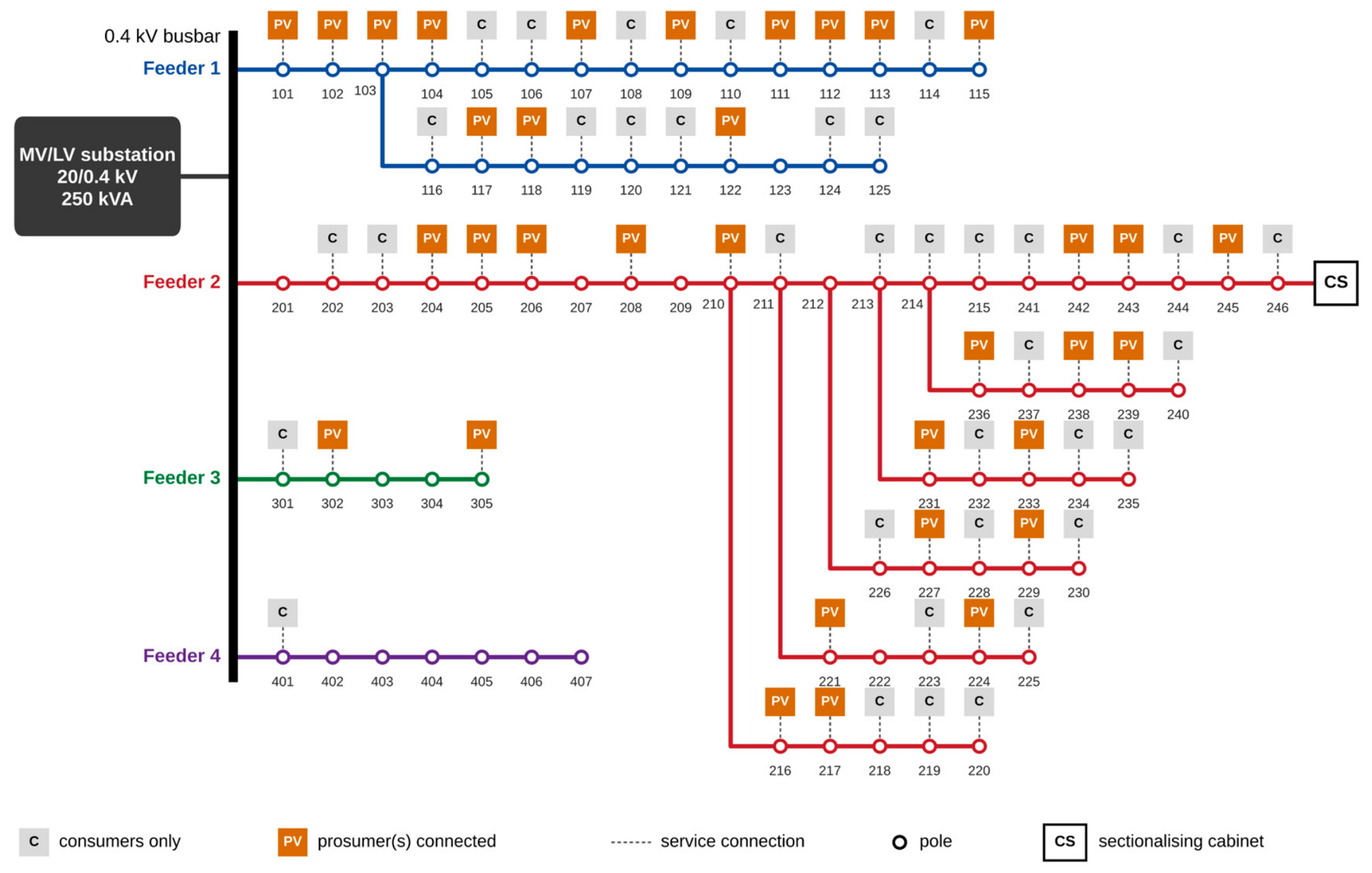
Figure 2.
Measured demand and photovoltaic export profiles.
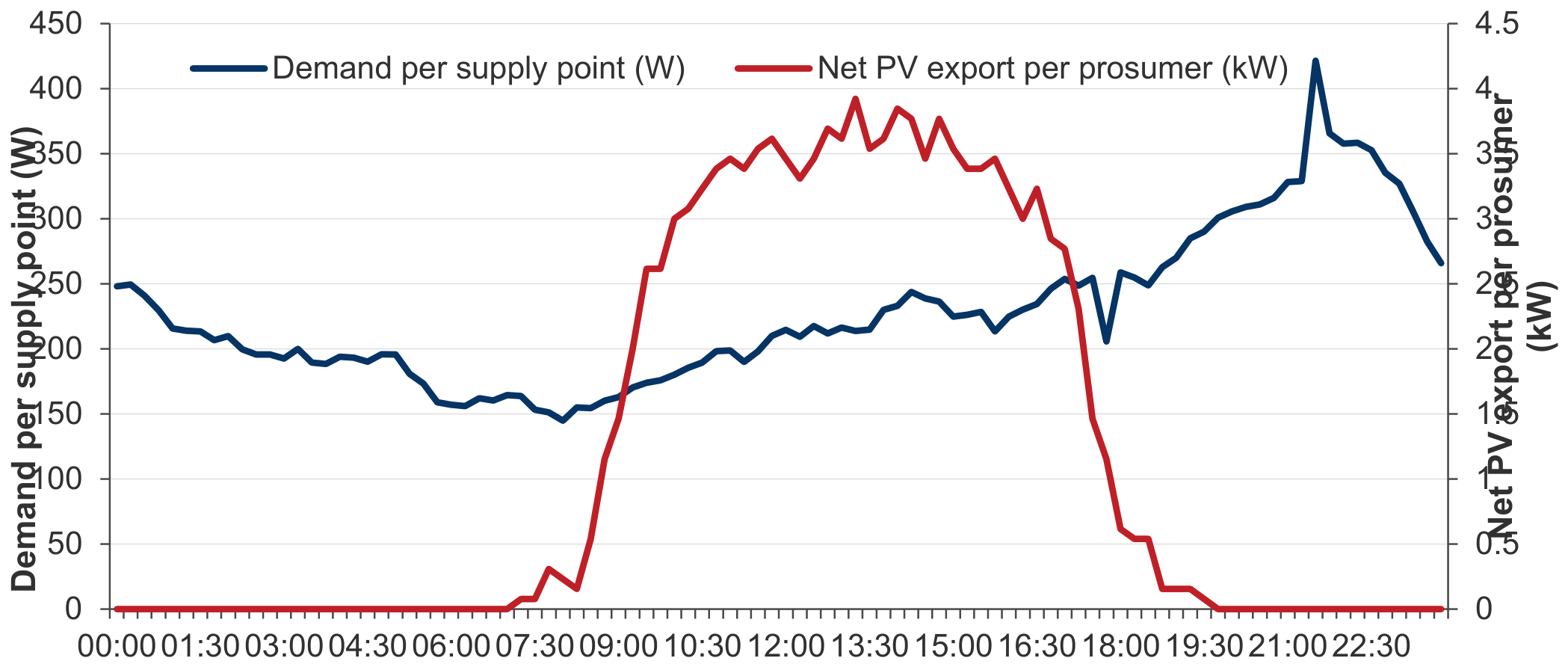
Figure 3.
Signed sensitivity of the critical node to each prosumer.
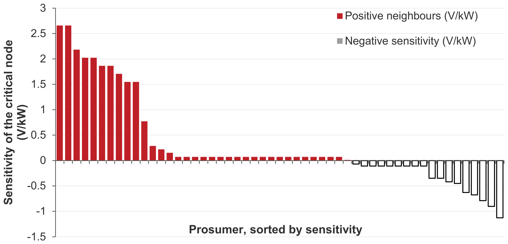
Figure 4.
Maximum network voltage over the day.
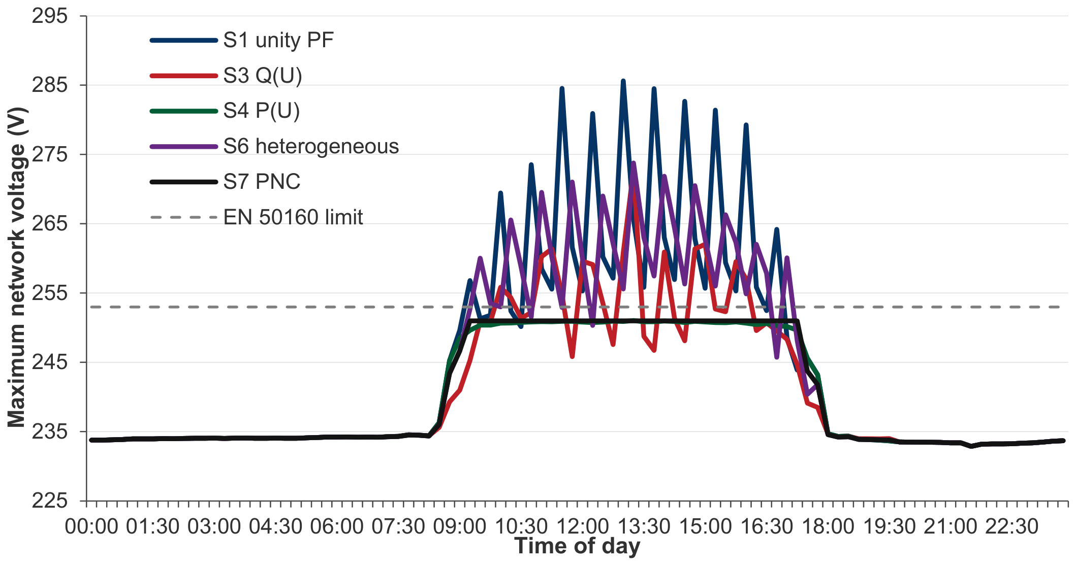
Figure 5.
Phase voltages at the critical node under S1.
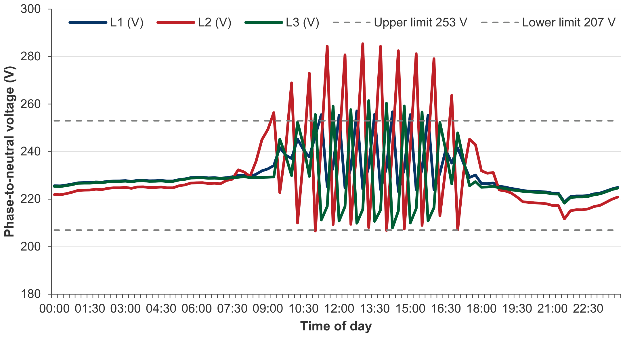
Figure 6.
Hosting capacity by control strategy.
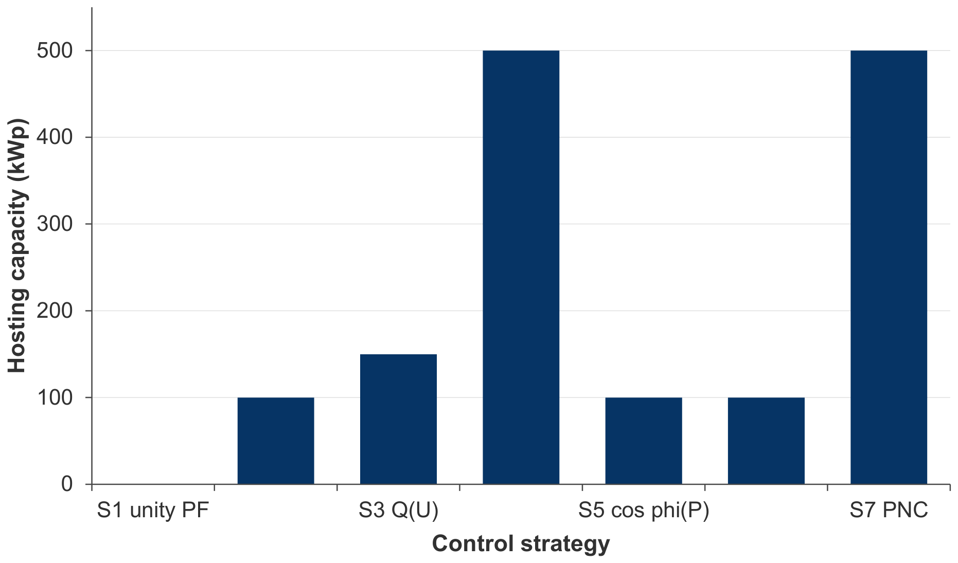
Figure 7.
Delivered photovoltaic energy against installed capacity.
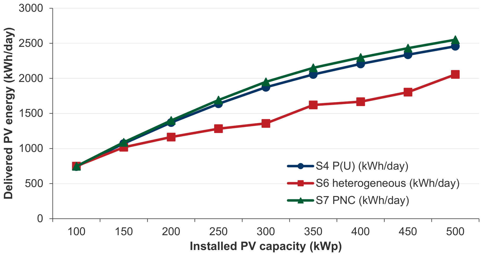
Figure 8.
Maximum network voltage against span length.
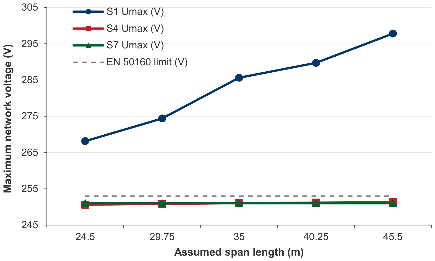
Figure 9.
Maximum network voltage for three prosumer phase allocations.
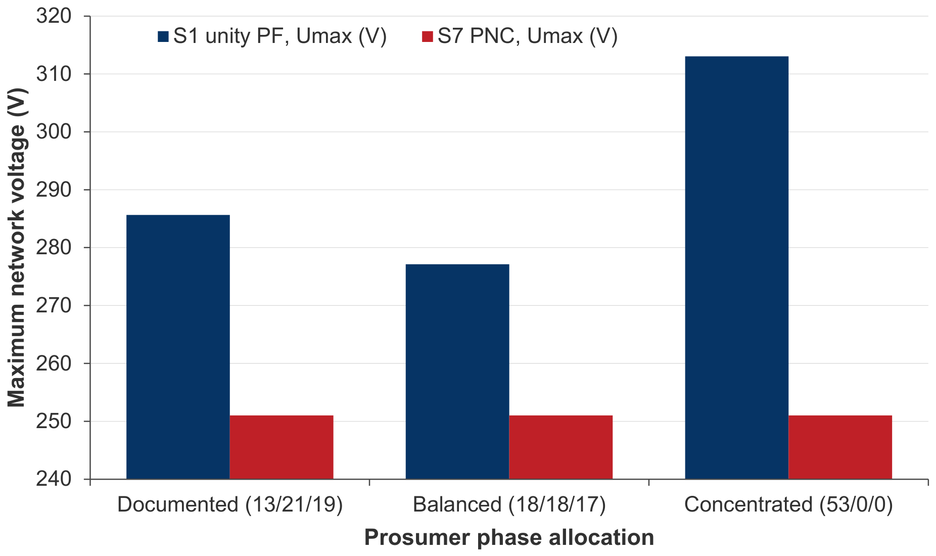
Figure 10.
Trade-off between voltage margin and curtailed energy in PNC.
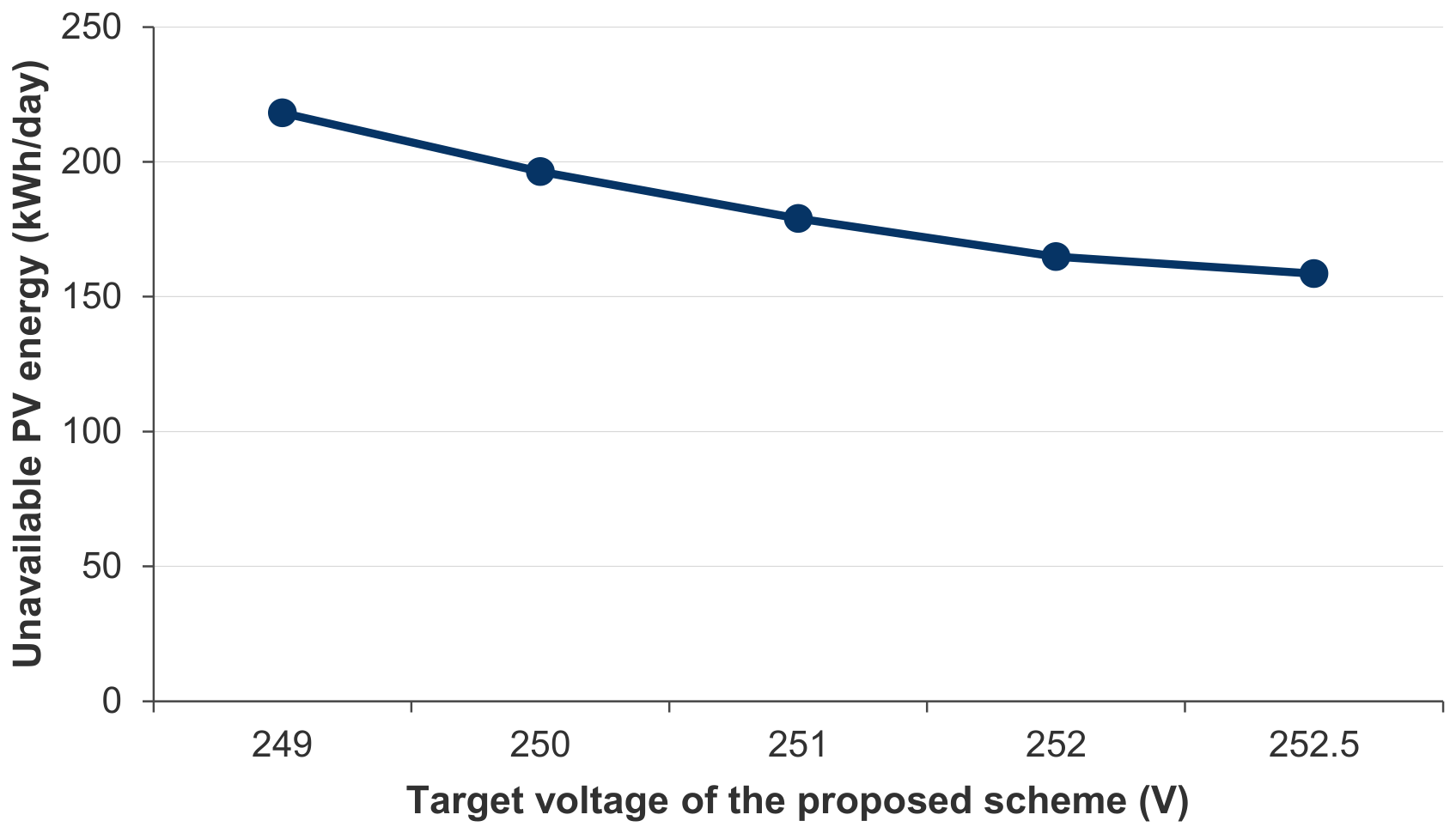
Table 1.
Positioning of the present work against the closest studies.
| Study | Four-wire | Real network | Documented phases | Time series | Protection dynamics | Signed sensitivity | Coordinated curtailment |
| [2,3] reviews | partly | various | no | partly | no | no | no |
| [22] 4-wire OPF | yes | no | no | yes | no | no | yes |
| [23] HC envelope | yes | yes | no | yes | no | no | no |
| [24] VUF analysis | yes | yes | partly | yes | no | no | no |
| [14] decentralised fairness | yes | no | no | yes | no | magnitude only | no |
| [16] centralised fairness | yes | yes | no | yes | no | magnitude only | yes |
| [30] single/three-phase PV | yes | no | no | no | no | observed, not derived | no |
| The proposed approach | yes | yes | yes | yes | yes | derived and used | yes |
Table 2.
Inverter control strategies. Un = 230 V.
| Case | Strategy | Definition |
| S0 | No photovoltaics | Reference network state, demand only |
| S1 | Unity power factor | Q = 0 at all times |
| S2 | Fixed power factor | cos φ = 0.95 underexcited, proportional to P |
| S3 | Q(U) droop | Deadband ±2% Un, linear to cos φ = 0.9 at ±8% Un |
| S4 | P(U) droop | Full output to 248 V, linear to zero at 253 V |
| S5 | cos φ(P) | Unity below 0.5 Pn, linear to 0.95 at Pn |
| S6 | Heterogeneous fleet | 40% S1, 20% S2, 20% S3, 20% S4 |
| S7 | Trip-aware PNC | S6 local laws plus operator power ceiling |
Table 3.
Characteristics of the S-NE test system.
| Quantity | Value |
| Transformer | 250 kVA, 20/0.4 kV, Dyn11, fixed tap +2.5% |
| Short-circuit impedance (LV side) | 8.25 + j24.00 mΩ (uR = 1.30%, uX = 3.78%) |
| Feeders / poles | 4 / 83 (25, 46, 5, 7) |
| Longest electrical path | 0.750 km (end of Feeder 2) |
| Supply points | 213 (203 single-phase, 10 three-phase) |
| Single-phase share | 95.3% |
| Supply points per feeder | 71 / 130 / 7 / 5 |
| Phase allocation of single-phase points (L1/L2/L3) | 66 / 71 / 66 |
| Prosumers | 53 (27 on F1, 24 on F2, 2 on F3) |
| Prosumer phase allocation (L1/L2/L3) | 13 / 21 / 19 |
| Measured busbar voltage (L1/L2/L3) | 234.45 / 234.67 / 235.69 V |
| Measured voltage unbalance factor | 0.07–0.59% |
| Aggregate demand (measured week) | peak 202.3 kW, mean 55.2 kW, peak/mean 3.66 |
| Net PV export per prosumer | 3.92 kW peak, 29.3 kWh on a clear day |
Table 4.
Conductor parameters.
| Conductor | r (Ω/km) | x (Ω/km) | rn (Ω/km) | X/R | Use |
| TYIR 50 OL-Al + 3×50+16 Al | 0.641 | 0.083 | 0.600 | 0.13 | F1 lateral |
| TYIR 50 OL-Al + 3×70+16 Al | 0.443 | 0.081 | 0.600 | 0.18 | F1–F4 overhead |
| NFA2X 50 OL-Al + 3×95+25 Al | 0.320 | 0.079 | 0.600 | 0.25 | F2 trunk head |
| AC2XABY 3×70+35 mm² | 0.443 | 0.077 | 0.868 | 0.17 | F1 cable head |
| NA2XABY 3×150+70 mm² | 0.206 | 0.072 | 0.443 | 0.35 | F2, F3 cable heads |
Table 5.
Change in phase-to-neutral voltage at the end of Feeder 2 for 5 kW injected on phase L1, as a function of the injection power factor (underexcited, absorbing reactive power).
Table 5.
Change in phase-to-neutral voltage at the end of Feeder 2 for 5 kW injected on phase L1, as a function of the injection power factor (underexcited, absorbing reactive power).
| cos φ | ΔU on L1 (V) | ΔU on L2 (V) | ΔU on L3 (V) |
| 1.00 | +16.08 | −6.41 | −2.90 |
| 0.97 | +15.15 | −8.38 | −0.42 |
| 0.95 | +14.85 | −8.98 | +0.36 |
| 0.90 | +14.23 | −10.17 | +1.93 |
| 0.85 | +13.67 | −11.19 | +3.30 |
Table 6.
Results of the reference case for all eight strategies.
| Case | Umax (V) | Umin (V) | >253 V | <207 V | Trips | Unavailable (kWh) | % | Jain |
| S0 no PV | 234.28 | 211.46 | 0 | 0 | 0 | — | — | — |
| S1 unity PF | 285.63 | 206.61 | 26 | 2 | 308 | 422.0 | 27.1 | 0.929 |
| S2 cos φ 0.95 | 280.87 | 203.84 | 25 | 6 | 184 | 249.8 | 16.1 | 0.949 |
| S3 Q(U) | 272.77 | 211.46 | 15 | 0 | 107 | 148.1 | 9.5 | 0.979 |
| S4 P(U) | 251.05 | 211.46 | 0 | 0 | 0 | 141.4 | 9.1 | 0.972 |
| S5 cos φ(P) | 269.02 | 202.04 | 19 | 7 | 205 | 279.9 | 18.0 | 0.935 |
| S6 heterogeneous | 273.80 | 203.39 | 27 | 4 | 262 | 351.4 | 22.6 | 0.936 |
| S7 PNC | 251.00 | 211.46 | 0 | 0 | 0 | 108.9 | 7.0 | 0.987 |
Table 7.
Effect of inverter oversizing on strategy S3, reference case. Unavailable energy falls monotonically with reactive headroom; the maximum voltage does not, because it is set by trip and reconnect cycling rather than by the steady-state droop.
Table 7.
Effect of inverter oversizing on strategy S3, reference case. Unavailable energy falls monotonically with reactive headroom; the maximum voltage does not, because it is set by trip and reconnect cycling rather than by the steady-state droop.
| Sn / Pn | Umax (V) | Trips | Unavailable energy (kWh) |
| 1.00 | 275.15 | 135 | 189.2 |
| 1.05 | 281.23 | 120 | 166.8 |
| 1.10 | 272.77 | 107 | 148.1 |
| 1.20 | 263.17 | 98 | 137.0 |
Table 8.
Maximum network voltage (V) against installed capacity, and the resulting hosting capacity. The transformer rating is 250 kVA, so the upper end of the sweep is twice the substation rating.
Table 8.
Maximum network voltage (V) against installed capacity, and the resulting hosting capacity. The transformer rating is 250 kVA, so the upper end of the sweep is twice the substation rating.
| Installed (kWp) | 100 | 150 | 200 | 250 | 300 | 350 | 400 | 450 | 500 | HC (kWp) |
| S1 | 253.4 | 266.0 | 280.8 | 288.3 | 306.1 | 322.1 | 326.5 | 312.8 | 337.6 | <100 |
| S2 | 249.9 | 258.4 | 276.2 | 288.9 | 305.5 | 308.4 | 331.1 | 332.6 | 341.5 | 100 |
| S3 | 246.1 | 251.3 | 267.2 | 275.0 | 296.7 | 303.9 | 300.2 | 303.9 | 329.9 | 150 |
| S4 | 249.1 | 250.4 | 251.0 | 251.3 | 251.7 | 251.9 | 252.1 | 252.3 | 252.5 | 500 |
| S5 | 249.9 | 260.8 | 267.8 | 289.3 | 301.7 | 313.4 | 341.0 | 336.0 | 340.6 | 100 |
| S6 | 252.0 | 260.1 | 272.3 | 289.9 | 301.9 | 332.2 | 326.6 | 337.3 | 354.4 | 100 |
| S7 | 250.9 | 251.0 | 251.0 | 251.0 | 251.0 | 251.5 | 252.0 | 252.4 | 252.7 | 500 |
Table 9.
Delivered photovoltaic energy (kWh/day) for the three strategies that curtail active power.
Table 9.
Delivered photovoltaic energy (kWh/day) for the three strategies that curtail active power.
| Installed (kWp) | 100 | 150 | 200 | 250 | 300 | 350 | 400 | 450 | 500 |
| S4 P(U) | 742 | 1071 | 1370 | 1638 | 1873 | 2055 | 2205 | 2337 | 2457 |
| S6 heterogeneous | 748 | 1018 | 1163 | 1283 | 1358 | 1621 | 1667 | 1803 | 2057 |
| S7 PNC | 748 | 1089 | 1399 | 1691 | 1950 | 2151 | 2298 | 2431 | 2551 |
| S7 over S4 (%) | +0.8 | +1.7 | +2.1 | +3.2 | +4.1 | +4.7 | +4.2 | +4.0 | +3.8 |
Table 10.
Jain fairness index J of the delivered energy fraction, and network losses P (kWh/day), across the penetration sweep.
Table 10.
Jain fairness index J of the delivered energy fraction, and network losses P (kWh/day), across the penetration sweep.
| Installed (kWp) | 100 | 200 | 300 | 400 | 500 |
| S4 J | 0.999 | 0.975 | 0.942 | 0.898 | 0.850 |
| S4 losses | 33.7 | 56.4 | 85.5 | 105.3 | 119.6 |
| S6 J | 1.000 | 0.937 | 0.922 | 0.921 | 0.931 |
| S6 losses | 35.7 | 65.0 | 107.8 | 175.3 | 249.8 |
| S7 J | 1.000 | 0.988 | 0.971 | 0.953 | 0.930 |
| S7 losses | 35.7 | 65.4 | 108.8 | 142.7 | 170.0 |
Table 11.
Sensitivity to the assumed span length, reference case. The uncontrolled maximum voltage moves by 30 V; the controlled cases move by less than 0.7 V and PNC not at all.
Table 11.
Sensitivity to the assumed span length, reference case. The uncontrolled maximum voltage moves by 30 V; the controlled cases move by less than 0.7 V and PNC not at all.
| Length factor | Span (m) | S1 Umax (V) | S4 Umax (V) | S7 Umax (V) | S7 unavailable (kWh) |
| 0.70 | 24.5 | 268.14 | 250.62 | 251.00 | 56.7 |
| 0.85 | 29.8 | 274.40 | 250.86 | 251.00 | 82.6 |
| 1.00 | 35.0 | 285.63 | 251.05 | 251.00 | 108.9 |
| 1.15 | 40.2 | 289.73 | 251.19 | 251.00 | 130.6 |
| 1.30 | 45.5 | 297.83 | 251.31 | 251.00 | 151.4 |
Table 12.
Sensitivity to the phase allocation of the 53 documented prosumers, reference case.
| Prosumer phase allocation |
S1 Umax (V) |
S1 Umin (V) |
S4 unavailable (kWh) | S7 unavailable (kWh) |
| Documented (13/21/19) | 285.63 | 206.61 | 141.4 | 108.9 |
| Balanced (18/18/17) | 277.13 | 207.72 | 78.5 | 70.8 |
| Concentrated (53/0/0) | 313.06 | 183.20 | 927.4 | 883.5 |
Disclaimer/Publisher’s Note: The statements, opinions and data contained in all publications are solely those of the individual author(s) and contributor(s) and not of MDPI and/or the editor(s). MDPI and/or the editor(s) disclaim responsibility for any injury to people or property resulting from any ideas, methods, instructions or products referred to in the content. |
© 2026 by the authors. Licensee MDPI, Basel, Switzerland. This article is an open access article distributed under the terms and conditions of the Creative Commons Attribution (CC BY) license (http://creativecommons.org/licenses/by/4.0/).
Copyright: This open access article is published under a Creative Commons CC BY 4.0 license, which permit the free download, distribution, and reuse, provided that the author and preprint are cited in any reuse.