

Submitted:
13 November 2026
Posted:
16 November 2026
You are already at the latest version
Abstract
Rain-on-grid models of small Mediterranean catchments require a loss model, usually the SCS Curve Number (SCS-CN) or the Green-Ampt (GA) methods, rarely tested inside two-dimensional solvers. This study compares the two methods as implemented in the same TUFLOW HPC model of the Aron stream (37.5 km², southern Italy), for the multi-pulse flood of 12–13 February 2026, under radar and rain-gauge forcing. Lacking discharge data, the comparison is evaluated on a sensitivity analysis of 24 runs varying the antecedent runoff condition (ARC) and the initial abstraction for SCS-CN, the initial water content, texture source, spin-up and saturated conductivity (Ks) for GA, and roughness. The SCS-CN peak varied 6- to 12-fold across ARC classes. Conversely, the GA peak varied by only 4% across initial water contents, since crest rainfall exceeded the GA capacity about tenfold, but decreased by 28–77% for a threefold to tenfold Ks, its dominant uncertainty. Despite producing similar overall volumes, the initial discharge peak reached only 2–8% of the main peak under ARC III and 35–44% with the GA spin-up. Additionally, GA reinfiltrated 12–18% of losses as run-on flow, a process absent in SCS-CN. Surface velocities confirmed only crest timing. Thus, a single SCS-CN simulation is not conservative for multi-pulse floods.
Keywords:
rain-on-grid
; direct rainfall
; infiltration
; SCS curve number
; Green-Ampt
; antecedent run-off condition
; weather radar
; TUFLOW HPC
; surface velocity
1. Introduction
Rain-on-grid modelling approaches integrate hydrologic and hydraulic processes by solving the two-dimensional (2D) shallow water equations across the entire catchment domain. Rainfall is applied to every computational cell, and the loss model governs both the timing and volume of effective precipitation that transitions into surface runoff [1]. In the steep Tyrrhenian catchments of Calabria, with areas of a few tens of km2 and response times of a few hours, loss parameters are rarely measured. They are usually taken from land-cover tables or from soil-texture classes. Thus, the loss model becomes a major, and seldom quantified, source of uncertainty in flood hazard mapping [2,3].
The SCS Curve Number (SCS-CN) method [4] is by far the most widely used loss model in engineering practice. It needs only one parameter per cell, derived by standard land-use and hydrologic soil group tables. In Italy, this spatial input is readily available through the national FOCA map [5]. However, the limitations of the SCS-CN method are well documented in the literature [6]. Specifically, the method relates cumulative runoff to cumulative rainfall, regardless of rainfall intensity, and its output is highly sensitive to the antecedent runoff condition (ARC, formerly AMC) and to the initial abstraction ratio (λ) [7].
Alternatively, the Green–Ampt (GA) model offers a physically based framework [8]. It computes the infiltration capacity as a function of saturated hydraulic conductivity, wetting-front suction head, and moisture deficit, thereby explicitly capturing the intensity and temporal dynamics of rainfall events [9]. Although its hydraulic parameters can be estimated from soil texture classifications [10], soil texture mapping is typically coarse, and the initial soil moisture state at the onset of a storm is rarely known a priori.
Direct comparisons between the two loss models are scarce in the literature. In a small agricultural catchment in Senegal, Bouvier et al. [11] found that a calibrated distributed SCS model outperformed GA, which exhibited high sensitivity to saturated hydraulic conductivity. However, that comparison, like most of the available ones, relied on hydrological models that compute infiltration losses independently of surface hydrodynamics. Within 2D shallow water solvers, Fernández-Pato et al. [12] calibrated the infiltration parameters of the Horton and GA laws against observed hydrographs. Nevertheless, a controlled comparison of SCS-CN and GA, under identical hydrodynamics, terrain and forcing, is still lacking.
To address this gap, this study provides a comparison of the two models on an observed multi-pulse storm event. Specifically, we investigate three key aspects of their behavior: first, the relative sensitivity of peak discharge to initial state parameters (initial soil moisture in GA versus antecedent runoff condition in SCS-CN); second, how the reliance of SCS-CN on cumulative rather than instantaneous rainfall shifts runoff from early pulses toward the main flood crest at equivalent runoff volumes; and third, how computing infiltration inline within the 2D solver leads to distinct run-on dynamics, as quantified through the domain water balance.
The second objective of this study was to evaluate the utility of a non-contact surface velocity record in constraining model behavior in a catchment without discharge data. The test case is the flood of 12–13 February 2026 on the Aron stream (Cetraro, Italy; 37.5 km2).
Infiltration via the SCS-CN and GA methods was computed by the soil module of the same TUFLOW HPC model, with identical terrain, roughness, boundaries and forcing, in 18 runs under two rainfall forcings (gauge-adjusted radar and a local rain gauge), alongside 6 parameter sensitivity runs. To isolate the intrinsic response of the infiltration equations from their hydrodynamic coupling with surface flow, a point-scale GA calculation was additionally executed under identical rainfall forcing. For each forcing scenario, rainfall was held constant and only the loss model was varied.
2. Materials and Methods
2.1. Study Area and Observations
2.1.1. Aron Catchment
The Aron stream drains a 37.5 km2 catchment in the Catena Costiera and discharges into the Tyrrhenian Sea at Cetraro (Cosenza, Italy) (Figure 1). The catchment is characterized by steep hillslopes and a narrow valley floor; over its lowermost 2 km, the stream crosses a short coastal plain that ends in a sandy beach. The computational domain covers about 70 km2, including the catchment and the adjacent coastal strip, and rainfall is applied to 59.5 km2 of it.
The bedrock is dominated by metamorphic units. Phyllites and micaschists cover 37.0 km2 (53% of the domain) and gneiss 24.4 km2 (35%); dolomites, marbles, granitoids, sandstones, gravelly alluvium, pelitic-arenaceous units and minor lithologies make up the remaining 12% (ISPRA, Carta Litologica d’Italia 1:100,000). Broadleaved forest (oak, chestnut, beech) covers most of the catchment, whereas olive groves, mixed agriculture and urban fabric occupy the coastal plain (Corine Land Cover, CLC, 4th level).
2.1.2. UNICAL-DINCI Station and Velocity Record
The hydro-pluviometric station was installed by the University of Calabria, within the “Tech4You” project, at the municipal bridge of Castelluzzo (Cetraro, Italy), on the main stem 1.8 km upstream of the mouth (UTM 33N: 582023.65 E, 4374675.19 N) (Figure 1). It records rainfall at 1-min resolution and, every 5 min, the water stage and the surface current velocity, the latter measured by a Doppler surface velocity radar (SVR100A) mounted on the bridge. Stage readings, disturbed by reeds, were not used for magnitudes.
The model’s time origin, t = 0 h, is 12 February 2026 at 00:00 UTC+1, and all times in this work are given in UTC+1.
The station recorded 74.2 mm in 48 h on 12–13 February. The maximum hourly total was 15.8 mm (13 February, 05:00–06:00) and the maximum 5-min intensity was 45.1 mm h−1. The event was preceded by 44.4 mm on 10–11 February. Rain fell in four distinct pulses (P1–P4, Table 1), a feature that makes the event well suited to testing how each loss model distributes losses in time. Isolated logger anomalies (14 records of 1–3 min) were set to zero.
Prior to signal analysis, three non-physical outliers were removed from the 577 velocity values recorded on 12–13 February. Consecutive values scatter by about ±0.5 m s−1; therefore, a 35-min centered moving median filter (spanning 7 consecutive values) was adopted to smooth noise. The baseline pre-event velocity, taken as the median for t = 2–10 h, was 2.96 m s−1.
Two aspects of the velocity dataset restricted its application for quantitative model calibration. The baseline pre-event velocity was already about 3 m s−1, and rainfall raised it by 1.3 m s−1 at most (P3 window). Additionally, velocity response was also not monotonic with respect to rainfall forcing: despite receiving 35.1 mm of rain (three times P3), window P4 exhibited the lowest median velocity (3.24 m s−1). Because the maximum velocity during P4 (05:55) concurred with the observed peak stage (06:00), validating station clock accuracy, the velocity record was employed strictly for temporal validation rather than magnitude constraint.
2.2. Rainfall Forcing
Rainfall forcing was established using two distinct data sources: a gauge-adjusted radar product (R) and a local rain gauge series (G).
The radar dataset comprised the surface rainfall intensity product (SRI_adj) of the Italian Civil Protection Department (1 km, 5 min), which applies an hourly adjustment matrix based on approximately 4,500 rain gauges [13,14,15]. A total of 576 images covering 12–13 February were reprojected to UTM 33N, resampled to 5 m, masked with the rainfall polygon and integrated in time with the trapezoidal rule, since TUFLOW reads the rainfall depth per interval. All radar timestamps were shifted from UTC to UTC+1 to align with station observations. Missing radar data between 23:00 and 24:00 UTC on 11 February were set to zero, during which the local gauge recorded 1.0 mm.
For the station-based scenario, the 5-min rain gauge series (74.2 mm total) was applied uniformly across the 59.5 km2 rainfall polygon.
Figure 2 illustrates the temporal distribution of the 12–13 February 2026 rainfall forcing, showing the hourly rainfall intensity from the local gauge, the local 1 km2 radar grid cell, and the catchment-averaged radar, alongside their respective cumulative rainfall totals.
The two forcing datasets exhibited substantial differences in total depth, spatial distribution, and temporal pulse sequence: at the gauge location, the radar registered 59.0 mm (21% lower than the gauge observation), whereas the catchment-wide mean radar depth reached 101.4 mm (and 95.7 mm over the broader rainfall polygon). Notably, the radar captured a pronounced rainfall pulse between 16:00 and 17:00 that was absent in the station record.
2.3. Hydrodynamic Model
All simulations were conducted using the same TUFLOW HPC model setup (build 2026.0.0, GPU solver), which solves the 2D shallow water equations with a finite-volume scheme and an adaptive time step [16], holding all parameters constant across runs except for the soils file and the precipitative forcing.
The computational domain was discretized using 10 m square cells. This grid resolution is supported by Artiglieri et al. [17], who demonstrated in a comparable Calabrian basin that TUFLOW HPC outlet hydrographs exhibit low sensitivity to cell size (across 5, 10, and 20 m grids) compared to models like HEC-RAS 2D, which suffer peak reduction and temporal lag on coarser grids. Topographic features were preserved using Sub-Grid Sampling (SGS) to sample the 1 m LiDAR DTM at a 1 m target spacing, generating cell–specific stage–storage and face–conveyance relationships. Additionally, linear embankment openings along the coastal plain were explicitly enforced using 9 breaklines (comprising 18 surveyed elevation points) with cell width factors governing their effective 10 m widths.
The main riverbed was defined by buffering the regional drainage network according to Strahler stream order: 20 m for order 1 (11 reaches), 50 m for order 2 (5 reaches), and 100 m for order 3 (the 5 main stem reaches). The resulting polygon covered 1.18 km2 down to the mouth.
Surface roughness was specified a priori without calibration, setting Manning’s coefficient (n) to 0.045 s m−1ᐟ3 within the riverbed polygon and assigning land-cover values ranging from 0.035 s m−1ᐟ3 (permanent grassland) to 0.100 s m−1ᐟ3 (forest) across the remaining domain based on CLC classifications [18,19].
The initial and continuing precipitation losses were set to zero, so that all losses came from the soil module (Section 2.4).
Downstream boundary conditions were represented by an automatic stage–discharge (HQ) line along the shoreline with a 0.01 bed slope, omitting tide and surge effects. All runs were initialized from dry conditions at t = 0 h, with the exception of the spin-up scenario which commenced at t = −48 h. Model execution maintained a wet/dry depth threshold of 0.002 m, a maximum allowable time step of 2 s, and default HPC drying logic for infiltration in partially wet cells (drying depth of 0.0019 m).
Output time series were recorded at 5-minute intervals at both the catchment outlet and the monitoring station, whose velocity is the depth-averaged velocity of the 10 m cell containing the sensor. A 48-h run took 17–28 min on one GPU. Post-processing was performed in Python 3 with NumPy, pandas and Matplotlib.
2.4. Loss Models
Infiltration losses were computed by the TUFLOW soil module in every wet cell, at every time step, utilizing a spatial soil-ID map and a coupled soil properties file. Infiltration was set to zero across the main riverbed polygon for all simulations, while the coastal beach area retained its own fixed parameterization; consequently, parameter variations were restricted exclusively to hillslope soils.
The two models are not coupled with the surface flow in the same way. GA operates directly on the water depth in the cell, allowing both local precipitation and run-on flow from upslope cells to infiltrate (in the HPC mass balance this appears as a volume leaving the domain through the soil). Conversely, SCS-CN acts on the local rainfall applied to the cell, and the run-on infiltration term of the mass balance was zero in all the SCS-CN runs: run-on never infiltrated. This asymmetry is part of the comparison (Section 3.1).
2.4.1. SCS Curve Number
The SCS-CN method determines cumulative runoff depth (Q), as a function of cumulative rainfall (P), from the start of the simulation:
where Ia = λS represents the initial abstraction, λ is typically 0.20 or 0.05, and S is the potential maximum soil moisture retention. The incremental loss per time step corresponds to the applied rainfall depth minus the change in Q.
In the SCS framework, ARC I, II, and III refer to the discrete antecedent runoff condition categories, representing dry, average, and wet initial moisture states, respectively, based on prior 5-day rainfall totals.
Baseline Curve Number (CN) values for average moisture conditions (CNII) were derived at a 250 m resolution from Italy’s national FOCA map [5] and extended across the model domain (outside the catchment its values are mostly CNII = 66). Figure 3a shows CNII from the FOCA map (250 m) over the forcing area. CNI and CNIII, for dry and wet moisture conditions, respectively, were evaluated following Chow et al. [20]:
For scenarios evaluating λ = 0.05, CNII values were re-scaled to maintain retention storage consistency with reduced initial abstraction [7], expressing S in inches:
Across the catchment, CNII values range from 25 to 88, yielding corresponding ranges of 12 to 75 for CNI and 43 to 95 for CNIII. The beach area was classified under hydrologic soil group D (sand with a shallow water table) with a fixed CNII of 90.
2.4.2. Green-Ampt
The Green–Ampt model expresses infiltration capacity (f), as a function of cumulative infiltration depth (F):
where Ks is the saturated hydraulic conductivity, ψ is the wetting-front suction head, and Δθ = θe − θi represents the available moisture deficit, defined by the effective porosity (θe) and initial volumetric water content (θi). A total soil mantle thickness of 1.0 m bounds the storage capacity at 1.0 m × Δθ, with surface runoff generated only when the combined rate of rainfall and upslope run-on exceeds f.
Soil hydraulic parameters (ψ, Ks, and θe) were assigned to each lithological class (Table 2, Figure 3b) based on the USDA soil texture of its weathered mantle [10], yielding an area-weighted domain Ks of 2.5 mm h-1. Initial soil moisture states (dry, medium, wet) correspond to water contents at suction heads of −1500 kPa (wilting point) and −33 kPa (field capacity) [21], with the medium state set to their arithmetic mean. All moisture values were converted to an effective basis, θi = θ − (η − θe) (where η is total porosity), to ensure consistency with θe. Cells unmapped by lithology were assigned clay loam properties, while the beach area was maintained at a constant wet condition (θi = 0.35).
2.5. Spin-Up and Sensitivity Configurations
To represent antecedent rainfall-driven moisture conditions, a 48-hour spin-up scenario was executed commencing on 10 February at 00:00 (t = −48 h) initialized at medium θi. During this pre-event window, 44.4 mm of antecedent rainfall infiltrated and routed through the catchment. Because TUFLOW does not explicitly simulate soil moisture recovery or evapotranspiration during inter-storm dry periods, the moisture state at t = 0 h represents the wettest compatible with the observed rainfall. This spin-up scenario serves as the physically based counterpart to ARC III, as the 5-day antecedent total (44.4 mm) exceeds the dormant-season ARC III threshold of 27.9 mm [4].
To evaluate parameter sensitivity to soil data sources, two regional datasets, i.e., LUCAS [22] and SoilGrids 2.0 [23], were sampled on a 25 m grid. The LUCAS dataset classifies 92% of the domain as loam (23.1% clay, 41.3% sand), whereas SoilGrids 2.0 assigns clay loam (31.2% clay, 30.7% sand) domain-wide. Within the GA scheme, these correspond to Ks values of 3.4 mm h-1 or 1.0 mm h-1 and ψ values of 89 mm or 209 mm, respectively. The lithology-based mapping agrees with SoilGrids 2.0 across phyllites and with LUCAS across gneissic units (together covering 88% of the domain).
An additional sensitivity scenario (GA uniform loam) assigned loam properties domain-wide (ψ = 88.9 mm, Ks = 3.4 mm h−1, θe = 0.434, θi = 0.165), isolating the texture source and its spatial distribution.
Finally, to decouple the intrinsic mathematical response of the infiltration formulations from 2D surface hydrodynamic interactions, GA infiltration was solved at a point, driven by the 5-min gauge rainfall, with the clay loam and loam parameters of Table 2 and the four initial states. Excess rainfall above infiltration capacity was immediately removed (preventing ponding and run-on). The same rainfall was applied to the SCS-CN model for CNII = 66 (the dominant domain value) under ARC I, II, and III conditions.
2.6. Experimental Design and Evaluation Metrics
The simulation matrix consists of 18 runs, with 9 dedicated to each rainfall forcing (Table 3).
The numerical experiment centers on two main pairings. The CN III and GA spin-up runs both account for the 44.4 mm of antecedent rainfall: SCS-CN through the tabulated ARC III class, GA by simulating that rainfall from t = −48 h. Conversely, the CN II and GA medium runs both ignore it and take the average initial state of each method: ARC II for SCS-CN and the medium θi of Table 2 for GA, as a designer would do without information on soil moisture. Additional model runs capture the parameter-induced uncertainty inherent to each approach.
Six supplementary radar-forced simulations evaluate sensitivity to parameters held constant in the primary matrix: Manning’s n multiplied by 0.8 and 1.2 for CN III and GA medium, which reflects the uncertainty of tabulated values [18,19], and Ks multiplied by 3 and 10 for GA medium on all hillslope soils, which spans the gap between texture-based values and the higher conductivities typical of forest topsoils.
In the absence of a stage-discharge rating curve at the monitoring station, direct discharge validation was not feasible. The runs were compared through model-internal indicators at the catchment outlet section: the peak discharge of the main crest (t ≥ 20 h) and its corresponding time to peak; the peak discharges of the initial flow pulse, P1 (t = 10–15.5 h), and of the radar-induced pulse at 16–17 h (t = 15.5–21 h), as fractions of the main peak (RP1 and RP2, respectively); cumulative runoff volume (t = 0–48 h) and the runoff coefficient (C), evaluated using catchment rainfall of 101.4 mm (radar) and 74.2 mm (rain gauge); the water balance over the forcing area, from the HPC mass-balance output; the area with maximum depth h ≥ 0.1 m and ≥ 0.5 m outside the riverbed; and the cumulative mass error, required to stay below 1%.
Observed and simulated velocities represent different physical quantities: a surface point velocity on a reach with base flow, and the depth-averaged velocity of a 10 m cell in a channel that is dry at t = 0 h. Direct magnitude comparisons were consequently omitted. Instead, the observed increment Δv = ṽ − 2.96 m s−1, where ṽ is the 35-min median surface velocity, was evaluated against simulated velocities using three metrics. The first is timing: for each rainfall window P1–P4, the time of the simulated maximum minus that of the observed maximum. The second is the weight of the first pulse, expressed as the increment in P1 divided by the increment in P3, and in P4. The observed ratios are 0.63 and 0.82. Two references were used because the P4 response is doubtful (P4 received three times the rainfall of P3 but produced the lowest median velocity), and the simulated value was judged closer to the observations only if it was closer for both ratios. The third is the Pearson correlation between observed and simulated series for t = 6–40 h.
3. Results
All runs closed the mass balance with a cumulative error of 0.00%.
3.1. Water Balance
The initial-state parameter exerted a markedly stronger control on total infiltration in the SCS-CN model than in the GA formulation (Figure 4). With radar forcing, SCS-CN infiltration over the forcing area fell from 86.3 mm (ARC I) to 41.0 mm (ARC III), whereas GA infiltration declined by only 7.1 mm (from 42.1 mm under dry initial moisture to 35.0 mm under wet conditions). A comparable disparity was observed under gauge-based forcing, where total infiltration ranged by 32.4 mm in SCS-CN (70.2 to 37.8 mm) versus 6.5 mm in GA (31.0 to 24.5 mm).
A comparison between the GA spin-up and GA medium runs reveals that antecedent wetness via spin-up exerted a negligible effect on the event-scale response. Although 24.9 mm of the 44.4 mm antecedent rainfall infiltrated prior to t = 0 h, subsequent event infiltration reached 36.0 mm under radar forcing and 25.3 mm under gauge forcing, reflecting a reduction of merely 1.0 mm compared to the baseline simulation with medium θi.
A divergence between the two modelling approaches lies in the handling of surface flow dynamics. Run-on infiltration was zero in every SCS-CN run. In contrast, GA generated run-on infiltration accounting for 3.9–6.6 mm in simulations starting at t = 0 h and 8.0–8.9 mm in the spin-up runs, 12–18% of the total infiltration. Residual domain surface storage at t = 48 h was 0.5–1.7 mm in all the runs.
Beyond initial wetness states and local flow dynamics, soil texture spatial representation emerged as a primary driver of the hydrological response. Assuming a spatially uniform loam texture increased cumulative infiltration relative to the baseline GA medium-moisture run by 13.2 mm under radar forcing (50.3 vs. 37.1 mm) and by 11.3 mm under gauge forcing (37.6 vs. 26.3 mm), since over the phyllites (covering 53% of the domain) its Ks is 3.4 mm h−1 instead of 1.0 mm h−1. Consequently, uncertainty or selection in soil texture sources imparted roughly twice the impact on hydrological losses as variations in initial moisture content.
3.2. Hydrographs and Peak Discharge
Hydrograph timing was highly consistent across simulations: all model configurations predicted the primary discharge peak on 13 February between 06:00 and 06:55, with the sole exception of the CN I run under radar forcing, which produced its global maximum during a secondary peak at 10:05 (Figure 5, Table 4). The magnitude of the primary peak discharge exhibited high sensitivity to the ARC class, spanning a 5.8-fold range under radar forcing (26.5 to 153.4 m3 s−1) and a 12-fold range under gauge forcing (11.7 to 143.9 m3 s−1). In contrast, peak discharge across the four GA states parameterized with lithology-based soil properties varied by only 4% under both forcing mechanisms.
Under nominal conditions, peak discharge predicted by the GA medium exceeded that of the CN II run by a factor of 2.0 under radar forcing and 2.7 under gauge forcing. Differences diminished under wet initial conditions: the GA spin-up configuration exceeded the CN III configuration by 15% in peak flow and 7% in total runoff volume under radar forcing, and by 30% and 35%, respectively, under gauge forcing.
With λ = 0.05, the main peak decreased by 12% (radar) and 5% (gauge) due to lower converted CN values, while the radar pulse at 16–17 h doubled (RP2 = 0.25 against 0.11), because runoff starts after less cumulative rainfall.
The SCS-CN formulation demonstrated greater sensitivity to precipitation forcing structure than the GA model. Although catchment-averaged precipitation was 37% higher under radar forcing than gauge forcing (101.4 vs. 74.2 mm), the GA medium peak discharge was 5% lower under radar forcing, whereas the CN II peak was 28% higher. This divergence reflects distinct infiltration mechanics: GA peak flow responds primarily to short-term rainfall intensity during the peak burst, which remained comparable between the two forcings (16.9 and 15.8 mm h−1 in the maximum clock hour), whereas SCS-CN peak discharge depends heavily on the rainfall accumulated since the start of the event.
3.3. Early Flow Peaks
The primary divergence between the two loss models lies in the temporal distribution of surface runoff across successive precipitation pulses. During the initial flow pulse (P1; 12 February, 13:00–14:00 h), peak flow reached 27–35% of the primary peak magnitude in the GA radar simulations and 40–44% in the gauge simulations (Figure 6a). In contrast, the SCS-CN model generated negligible initial response, accounting for only 1–4% (radar) and 3–8% (gauge) of the primary peak, with the elevated value of 19% under the CN I gauge run attributable to its exceptionally low primary peak. Furthermore, the subsequent radar pulse at 16:00–17:00 h, absent in the gauge observations, yielded runoff peak ratios RP2 = 0.85–0.88 for GA compared to 0.11–0.45 for SCS-CN (Table 4).
Within SCS-CN, RP2 increases with the ARC class (0.11 to 0.45, radar), since a wetter class shortens the rainfall needed before runoff starts; RP1 stays below 0.05 except in the CN I gauge run. Conversely, GA pulse ratios demonstrated minimal sensitivity to initial conditions, varying by at most 0.06 across states. Consequently, in Figure 6b, it is possible to note that GA simulations formed a tightly bounded cluster (C = 0.48–0.64, Qp = 165–188 m3 s−1). By contrast, SCS-CN responses exhibited broad dispersion along both axes, with individual run placement governed primarily by ARC classification rather than structural model dynamics.
3.4. Point-Scale Behavior
At the point scale, GA infiltration capacity remained an order of magnitude below the rainfall intensity at the flood crest (Figure 7a). At t = 30 h, infiltration capacity ranged across initial states from 2.2 to 2.9 mm h−1 for clay loam and 5.0 to 6.0 mm h−1 for loam, whereas maximum 60-min rainfall depth reached 21.5 mm and peak 5-min intensity reached 45.1 mm h−1. Total event-scale point infiltration for dry, medium, and wet initial states was 33.5, 31.0, and 27.9 mm for clay loam, and 46.5, 44.4, and 41.9 mm for loam, respectively (Figure 7b). In contrast, SCS-CN simulations (CNII = 66) yielded total infiltration losses of 73.8, 61.3, and 41.2 mm across antecedent runoff conditions ARC I, II, and III.
The spin-up dynamics exhibited pronounced scale dependence. At the point scale, antecedent precipitation infiltration reached 29.0 mm for clay loam and 38.9 mm for loam, which subsequently reduced event infiltration relative to the medium moisture state by 11.5 mm (37%) and 9.0 mm (20%), respectively (Figure 7b). On the contrary, in the 2D spatial model, spin-up reduced event infiltration by merely 1.0 mm (Figure 7c). The 2D model infiltrated only 1.2 mm of the initial light rainfall (2.3 mm cumulative for t < 6 h), whereas the 1D point-scale GA formulation completely absorbed this initial volume.
3.5. Velocity at the Station
Peak timing represented the most robust agreement between simulated hydrographs and streamflow observations (Figure 8). Across both radar- and gauge-based forcing datasets, peak velocity timing predicted by the GA and CN III model configurations closely matched the observed P4 maximum (05:55), with timing errors bounded within 0 to 15 min.
Hydrograph structure varied markedly across model formulations during the initial phase of the storm event. The GA model reproduced a distinct velocity response to the first pulse under both forcing mechanisms. Conversely, the SCS-CN framework failed to generate an initial response under CN II, reproducing it under CN III only when driven by gauge-based forcing.
Relative magnitude performance across pulses did not yield a single optimal model structure, as performance ranking depended on the selected reference pulse (Table 5): GA provided the closest match to observed peak ratios for P4 (0.60–0.70 simulated vs. 0.82 observed), whereas CN III agreed more closely for P3 (0.82–0.92 simulated vs. 0.63 observed). Overall event-scale hydrograph correlation remained weak across all model configurations (r ≤ 0.30).
Furthermore, note that, simulated depth-averaged peak flow velocities (1.60–2.65 m s−1, initialized from a dry channel state) could not be directly compared against the observed surface velocity of 3.95 m s−1 without adjusting for baseflow and applying a surface-to-mean velocity conversion coefficient.
3.6. Maximum Depth and Flooded Area
The inundation extent differed substantially between model formulations. The domain area outside the primary channel experiencing a maximum flow depth h ≥ 0.1 m ranged from 0.14 to 0.66 km2 in the SCS-CN simulations compared to 0.70 to 0.80 km2 under GA parameterizations (Table 4). For deeper inundation (h ≥ 0.5 m), the respective inundated areas spanned 0.003–0.107 km2 for SCS-CN and 0.085–0.129 km2 for GA.
Discrepancies in maximum flow depth were spatially concentrated along the main stem and its primary tributaries (Figure 9). Along the main channel between the principal confluence and the gauging station, the GA medium run yielded maximum depths up to 0.5 m greater than the CN II run. In contrast, spatial depth differences between the GA spin-up and CN III configurations remained below 0.2 m across nearly the entire domain. On the coastal plain, near the embankment openings and between the urban blocks, the sign of the difference alternates between adjacent cells. There the maximum depth depends on when and where local overflows occur, so small differences in the timing of the hydrograph shift water from one cell to another; the pattern does not indicate a larger flood volume in either model.
3.7. Sensitivity to Roughness and Saturated Conductivity
Hydraulic roughness exerted a minor influence on discharge hydrographs but significantly affected flow velocity (Table 6). A ±20% change in n altered primary peak discharge by only 1–2% and shifted early-pulse runoff peak ratios by at most 0.05. Conversely, peak channel velocity at the gauging station varied by approximately ±11% (ranging between 2.27 and 2.80 m s−1 for CN III, and 2.38 to 2.89 m s−1 for GA medium), more than the difference between the two models at nominal roughness (0.10 m s−1). Peak timing exhibited a minor shift of up to 10 min. Total inundation extent scaled positively with n, resulting in overlapping flooded area ranges between the two model formulations (0.60–0.72 km2 for SCS-CN vs. 0.65–0.78 km2 for GA).
Hydrological response in the GA formulation was predominantly governed by Ks. Tripling Ks reduced primary peak discharge by 28% and halved total runoff volume, whereas a tenfold increase in Ks reduced peak discharge and runoff volume by 77% and 90%, respectively, corresponding to an increase in total infiltration from 37.1 to 89.6 mm. Across this spectrum of hydraulic conductivity values, GA peak discharge ranged from 41 to 175 m3 s−1 (a 4.3-fold factor), exhibiting sensitivity comparable to the 5.8-fold variation observed across SCS-CN ARC classes. Runoff peak ratios also decreased markedly with increasing Ks: RP1 declined from 0.33 to 0.09 and 0.03, while RP2 dropped from 0.87 to 0.68 and 0.25. When Ks was increased threefold (Ks × 3), GA produced a total runoff volume closely matching that of CN II (1.11 × 10⁶ against 1.17 × 10⁶ m3) yet generated a 46% higher peak discharge and a substantially higher secondary peak ratio (RP2 = 0.68 vs. 0.11).
4. Discussion
4.1. Rainfall Intensity Dominance over Initial Moisture in GA Peak Response
During the peak of a rainfall event, the instantaneous runoff fraction (dQ/dP) in the GA model is expressed as 1 − f/i, where i is the rainfall intensity. Considering an infiltration capacity of 2–6 mm h−1 and 21.5 mm of precipitation in the maximum clock hour, this fraction varies from 0.72 to 0.90, with only 0.02-0.05 difference for different initial soil moisture conditions (Section 3.4). In contrast, the instantaneous runoff fraction in the SCS-CN model is the derivative of the cumulative runoff equation:
For CNII = 66 and 60 mm of cumulative precipitation before the peak burst, dQ/dP yields values equal to 0.00, 0.37, and 0.71 for ARC I, II, and III, respectively. The reason why dQ/dP values vary significantly between adjacent ARC types is because S changes by roughly 2.3–2.4 from one ARC class to the next (S = 312, 131, and 57 mm). Therefore, the ARC classification governs the proportion of the peak precipitation burst converted into surface runoff, whereas initial soil moisture (θi) in GA merely modulates an infiltration capacity that is already small relative to rainfall intensity.
This theoretical distinction highlights Ks as the critical parameter governing GA response. When baseline infiltration capacity is taken into account, variation in Ks can produce peak discharge variation comparable to that from ARC classification of SCS-CN (Section 3.7). Although GA peak does not depend on θi, the overall modelling uncertainty is of the similar magnitude within both models, as found for GA’s sensitivity to Ks by Bouvier et al. [11]. However, one should not make the generalization that θi does not influence the peak of GA; that dependency is associated with longer, less intense rainfall, coarser-texture soils, or when Ks is comparable to the rainfall intensity, since sorptive matrix suction then plays a higher part in infiltration losses, increasing the effect of initial moisture.
4.2. Temporal Redistribution of Losses
The cumulative infiltration loss in the SCS-CN model is dependent on cumulative precipitation only, therefore, initial periods of high rainfall are mostly retained by the land regardless of their intensity at the time. The GA formulation generates runoff when rainfall is higher than the infiltration capacity of the site even during the beginning of the storm. Although CN III and GA spin-up give runoff volumes within 7% of each other under radar forcing, the first pulse reaches 2% of the main peak with CN III and 35% with GA spin-up.
This structural divergence carries practical flood risk implications: an SCS-CN configuration calibrated to match the primary peak (e.g., using ARC III) still produces early flow peaks much smaller, relative to the main peak, than GA. Accurately resolving these early pulses is critical for estimating flood warning lead times and assessing pre-peak hydraulic loading, such as debris and sediment transport preceding the main crest. Observational evidence confirms an initial stream response, as indicated by a measured velocity increment during pulse P1; however, data limitations prevent a definitive empirical validation of which model structure better replicates the absolute magnitude of this initial pulse.
4.3. Coupling with the 2D Solver
The GA solution in the TUFLOW soil module takes into account both the infiltration of ponded water and run-on water resulting in water losses between 12% and 18% of the total infiltration losses. On the other hand, the SCS-CN formulation only deals with direct precipitation. The result is that a 2D SCS-CN rain-on-grid model effectively acts as a net-rainfall model: runoff leaving a cell cannot reinfiltrate downslope. To be precise, we are comparing loss models as applied within the solver technology, not the mere loss equations themselves; part of the difference in amount and initial peak flows comes from this decision and will therefore only be applicable to other 2D hydraulic modeling software where the run-on aspect is modeled identically to this solution.
Model spin-up reveals a secondary hydro-numerical coupling effect. Antecedent rainfall reduced the event infiltration by 9.0–11.5 mm at point scale and by 1.0 mm in the 2D model. Moreover, the two-dimensional models only permitted about one half of the total amount of the initial light rainfall to be infiltrated. Both of these findings indicate that, under the conditions of low rainfall intensity, the majority of the area-based infiltration loss on a steep hillslope comes from the amount of time that surface ponding exceeds the drying depth threshold (0.0019 m), rather than by the infiltration capacity. On steep gradients, this ponding time will be short. Additionally, the algorithmic scheme used by the solver to track and carry cumulative infiltration across dry intervals may attenuate the memory of antecedent wetting, a detail that could not be independently verified from available software documentation. In either case, the minor influence of model spin-up reflects an emergent property of the coupled hydro-numerical framework. Consequently, any method of spin-up used in rain-on-grid models must first be evaluated with a 1D point-scale analytical or numerical solution before it can be used to describe previous conditions.
4.4. Implications for Flood Hazard Mapping
Selecting different models for estimating losses and different classifications of ARC (Section 3.6) can result in large differences in the extent of flooding. Within the GA medium-moisture and CN II parameterizations (representative of what is an overall common use by engineers), the maximum difference in depth of the flow on the main stem of the river reached 0.5 meters. Across initial states the GA runs form a tight cluster, whereas the SCS-CN runs spread widely with the ARC class (Figure 6b). Across Ks, however, the spread of the GA results is comparable to that of SCS-CN (Table 7). Consequently, relying on a deterministic single-run configuration for either model imparts a false sense of precision, aligning with recent evaluations regarding the parameter uncertainty of rain-on-grid models in flood hazard mapping [2,3].
No single model configuration provides a universally conservative estimate across all flood hazard indicators. When parameterized using texture-based soil properties, the GA model produced the maximum peak discharge, runoff volume, and total inundation extent within the simulation matrix; however, these peak values decline sharply if Ks exceeds standard tabulated values. For flood hazard mapping applications, a robust practical workflow consists of executing the SCS-CN framework under antecedent runoff condition ARC III alongside GA simulations spanning a range of Ks multipliers surrounding baseline texture-based values (e.g., ×1 to ×3), subsequently mapping the spatial envelope of maximum water depths. In applications where early-pulse dynamics are critical (such as defining flood warning thresholds or evaluating pre-peak hydraulic blockage of culverts and bridges), the GA formulation is preferable, as SCS-CN attenuates initial hydrograph pulses during the early stages of an event.
4.5. Observational Constraints and Limitations
The velocity record validated the timing of the simulated velocity crest and confirmed an initial response to the first pulse; it did not confirm the simulated discharge magnitudes. The streamflow station is located in a reach that has a perennial baseflow, so pre-event flow velocities were approximately 3.0 m s−1 which will decrease the relative amount of event-driven velocity increases and reduce the magnitude of the event-driven velocity increases caused by the most intense precipitation burst (P4).
The surface velocity estimates derived from Doppler radar are very dependent upon the surface boundary conditions and the assumed relationship between surface velocity to the mean velocity [24]; intense precipitation on the water surface can introduce significant noise into the Doppler radar signal. It is therefore necessary, at the very least, to use surveyed channel cross-sections, high-water marks post-event, and a model initial condition that includes the pre-event baseflow to effectively differentiate between infiltration model structures from such remote sensing datasets.
It is important to mention that the results obtained in this study pertain specifically to this analyzed case. Specifically, we are dealing with a single multi-pulse winter storm, without discharge measurements, a surveyed cross-section at the bridge or flood marks.
As regards the numerical simulations, initializing the numerical domain with a dry channel bed at t = 0 h artificially inflated simulated velocity increments while delaying early hydrograph response. Another important point is that the hydraulic parameters derived from GA were determined on basis of soil types from mapped lithology and do not represent field measurements of saturated hydraulic conductivity. The soils of a forested area overlying metamorphic bedrock contain a relatively high portion of both macropores and coarse fragments (>20% of the soil mass as provided by LUCAS soil data), and these features significantly alter the values of Ks and apparent porosity. Furthermore, the TUFLOW does not recover the SCS-CN retention or the GA infiltration capacity during dry intervals, and it does not compute subsurface return flow. Lastly, sensitivity analysis for n (±20%) was limited to two configurations and to the 10 m grid, which resolves first-order channels with only two cells, where rain-on-grid results are grid-sensitive [25].
5. Conclusions
The SCS-CN and GA infiltration formulations were evaluated within a 2D TUFLOW HPC rain-on-grid hydrodynamic model applied to the Aron stream catchment during the multi-pulse flood event of 12–13 February 2026, driven by both radar and rain-gauge precipitation forcing.
Sensitivity analysis demonstrated that primary peak discharge varied by a factor of 6 to 12 across SCS-CN ARC classes, compared to a variation of only 4% across GA initial moisture states. During the main burst, at the flood crest, rainfall intensity exceeded GA infiltration capacity by an order of magnitude; consequently, initial soil moisture exerted minimal control on the instantaneous runoff fraction. For GA, saturated hydraulic conductivity represented the dominant controlling parameter: a 3-fold and 10-fold increase in Ks reduced peak discharge by 28% and 77%, respectively, producing a response spread comparable to that across SCS-CN ARC classes.
At comparable event-scale runoff volumes (agreeing within 7%), the initial flow pulse reached only 2–8% of the primary peak magnitude under SCS-CN (ARC III), compared to 35–44% under the GA spin-up configuration. This disparity arises because SCS-CN infiltration losses depend strictly on cumulative precipitation depth, thereby systematically attenuating early-stage hydrograph peaks. This structural contrast is pronounced for GA capacities typical of fine-textured soils (a few millimeters per hour) but diminishes when Ks is increased to ten times baseline tabulated values.
Hydro-numerical coupling within the solver further differentiated the two formulations. GA accounted for the reinfiltration of overland run-on, which contributed 12–18% of total infiltration losses, whereas SCS-CN operated strictly on direct precipitation. Additionally, antecedent wetting reduced event infiltration by 9.0–11.5 mm in 1D point-scale GA calculations, compared to merely 1.0 mm in the 2D spatial domain. This discrepancy suggests that 2D hillslope infiltration during low-intensity precipitation is constrained primarily by localized inundation residence time (infiltration opportunity) rather than hydraulic capacity.
Consequently, relying on a single deterministic SCS-CN simulation with a prescribed antecedent condition does not represent a universally conservative framework for multi-pulse flood events; such a setup may successfully reproduce the primary peak while strongly attenuating the early pulses.
Finally, non-contact Doppler velocity observations at the Castelluzzo gauging station constrained peak timing to within 15 min but lacked the diagnostic resolution to discriminate between model structures: a ±20% perturbation in Manning’s n induced an ±11% shift in peak flow velocity, a variation exceeding the baseline difference between the two loss models.
Author Contributions
Conceptualization, D.A.F., N.P. and R.G.; methodology, D.A.F. and N.P.; software, D.A.F.; validation, D.A.F. and N.P.; formal analysis, D.A.F.; investigation, D.A.F. and N.P.; resources, N.P. and R.G.; data curation, N.P.; writing—original draft preparation, D.A.F.; writing—review and editing, N.P. and R.G.; visualization, D.A.F.; supervision, R.G.; funding acquisition, R.G. All authors have read and agreed to the published version of the manuscript.
Funding
This work was funded by the Next Generation EU - Italian NRRP, Mission 4, Component 2, Investment 1.5, call for the creation and strengthening of “Innovation Ecosystems”, building “Territorial R&D Leaders” (Directorial Decree n. 2021/3277) - project Tech4You - Technologies for climate change adaptation and quality of life improvement, n. ECS0000009. This work reflects only the authors’ views and opinions, neither the Ministry for University and Research nor the European Commission can be considered responsible for them.
Data Availability Statement
Radar data (SRI_adj) are distributed by the Italian Civil Protection Department. Station data belong to the Department of Civil Engineering, University of Calabria, and are available from the corresponding author on reasonable request. Model files and scripts used for the analysis are available from the authors.
Acknowledgments
The authors thank the Italian Civil Protection Department for the radar data. During the preparation of this manuscript, the authors used Claude (Anthropic, claude.ai; model Claude Opus 5.5, accessed in October 2026) for the purposes of language editing and typographical correction, as well as assisting in writing the Matlab and Python scripts used to check the calculations. The authors have reviewed and edited the output and take full responsibility for the content of this publication.
Conflicts of Interest
The authors declare no conflicts of interest.
References
- Hall, J. Direct rainfall flood modelling: the good, the bad and the ugly. Australas. J. Water Resour. 2015, 19, 74–85. [Google Scholar]
- David, A.; Schmalz, B. Flood hazard analysis in small catchments: comparison of hydrological and hydrodynamic approaches by the use of direct rainfall. J. Flood Risk Manag. 2020, 13, e12639. [Google Scholar] [CrossRef]
- Costabile, P.; Costanzo, C.; Ferraro, D.; Barca, P. Is HEC-RAS 2D accurate enough for storm-event hazard assessment? Lessons learnt from a benchmarking study based on rain-on-grid modelling. J. Hydrol. 2021, 603, 126962. [Google Scholar] [CrossRef]
- USDA-NRCS. Urban Hydrology for Small Watersheds; Technical Release 55; United States Department of Agriculture, Natural Resources Conservation Service: Washington, DC, USA, 1986. [Google Scholar]
- Claps, P.; Evangelista, G.; Ganora, D.; Mazzoglio, P.; Monforte, I. FOCA: a new quality-controlled database of floods and catchment descriptors in Italy. Earth Syst. Sci. Data 2024, 16, 1503–1522. [Google Scholar] [CrossRef]
- Ponce, V.M.; Hawkins, R.H. Runoff curve number: has it reached maturity? J. Hydrol. Eng. 1996, 1, 11–19. [Google Scholar] [CrossRef]
- Hawkins, R.H.; Jiang, R.; Woodward, D.E.; Hjelmfelt, A.T.; Van Mullem, J.A. Runoff curve number method: examination of the initial abstraction ratio. In Proceedings of the Second Federal Interagency Hydrologic Modeling Conference, Las Vegas, NV, USA, 2002. [Google Scholar]
- Green, W.H.; Ampt, G.A. Studies on soil physics, 1. The flow of air and water through soils. J. Agric. Sci. 1911, 4, 1–24. [Google Scholar] [CrossRef]
- Mein, R.G.; Larson, C.L. Modeling infiltration during a steady rain. Water Resour. Res. 1973, 9, 384–394. [Google Scholar] [CrossRef]
- Rawls, W.J.; Brakensiek, D.L.; Miller, N. Green-Ampt infiltration parameters from soils data. J. Hydraul. Eng. 1983, 109, 62–70. [Google Scholar] [CrossRef]
- Bouvier, C.; Bouchenaki, L.; Tramblay, Y. Comparison of SCS and Green-Ampt distributed models for flood modelling in a small cultivated catchment in Senegal. Geosciences 2018, 8, 122. [Google Scholar] [CrossRef]
- Fernández-Pato, J.; Caviedes-Voullième, D.; García-Navarro, P. Rainfall/runoff simulation with 2D full shallow water equations: sensitivity analysis and calibration of infiltration parameters. J. Hydrol. 2016, 536. [Google Scholar] [CrossRef]
- DPC–CIMA. DataMet – Gestione e Produzione Dati della Rete Radar Nazionale; Italian Civil Protection Department and CIMA Research Foundation: Rome, Italy, 2018. [Google Scholar]
- Bruno, G.; Pignone, F.; Silvestro, F.; Gabellani, S.; Schiavi, F.; Rebora, N.; Giordano, P.; Falzacappa, M. Performing hydrological monitoring at a national scale by exploiting rain-gauge and radar networks: the Italian case. Atmosphere 2021, 12, 771. [Google Scholar] [CrossRef]
- Franch, G.; Tomasi, E.; Azhel, U.; Tomezzoli, G.; Camilletti, A.; Poli, V.; Pelosini, R.; Vulpiani, G.; Scipione, G.; Trotta, G.; Angelinelli, M. IT-DPC-SRI: A cloud-optimized archive of Italian radar precipitation (2010–2025). arXiv 2026, arXiv:2602.15088. [Google Scholar] [CrossRef]
- TUFLOW. TUFLOW Classic/HPC User Manual. 2026. Available online: https://docs.tuflow.com/classic-hpc/manual/2026.0/ (accessed on 22 October 2026). version 2026.0; BMT, .
- Artiglieri, P.; Curulli, G.; Coscarella, F.; Algieri Ferraro, D.; Macchione, F. Performance of HEC-RAS v6.5 at basin scale for calculating the flow hydrograph: comparison with TUFLOW. Nat. Hazards 2025, 121, 9477–9490. [Google Scholar] [CrossRef]
- Chow, V.T. Open-Channel Hydraulics; McGraw-Hill: New York, NY, USA, 1959. [Google Scholar]
- Arcement, G.J.; Schneider, V.R. Guide for Selecting Manning’s Roughness Coefficients for Natural Channels and Flood Plains; U.S. Geological Survey Water-Supply Paper 2339; USGS: Denver, CO, USA, 1989. [Google Scholar]
- Chow, V.T.; Maidment, D.R.; Mays, L.W. Applied Hydrology; McGraw-Hill: New York, NY, USA, 1988. [Google Scholar]
- Rawls, W.J.; Brakensiek, D.L.; Saxton, K.E. Estimation of soil water properties. Trans. ASAE 1982, 25, 1316–1320. [Google Scholar] [CrossRef]
- Ballabio, C.; Panagos, P.; Montanarella, L. Mapping topsoil physical properties at European scale using the LUCAS database. Geoderma 2016, 261, 110–123. [Google Scholar] [CrossRef]
- Poggio, L.; de Sousa, L.M.; Batjes, N.H.; Heuvelink, G.B.M.; Kempen, B.; Ribeiro, E.; Rossiter, D. SoilGrids 2.0: producing soil information for the globe with quantified spatial uncertainty. SOIL 2021, 7, 217–240. [Google Scholar] [CrossRef]
- Welber, M.; Le Coz, J.; Laronne, J.B.; Zolezzi, G.; Zamler, D.; Dramais, G.; Hauet, A.; Salvaro, M. Field assessment of noncontact stream gauging using portable surface velocity radars (SVR). Water Resour. Res. 2016, 52, 1108–1126. [Google Scholar] [CrossRef]
- David, A.; Schmalz, B. A systematic analysis of the interaction between rain-on-grid-simulations and spatial resolution in 2D hydrodynamic modeling. Water 2021, 13, 2346. [Google Scholar] [CrossRef]
Figure 1.
The Aron catchment: catchment boundary, rainfall forcing area, riverbed polygon, outlet section and UNICAL-DINCI station over a hillshade of the 1 m LiDAR DTM.
Figure 1.
The Aron catchment: catchment boundary, rainfall forcing area, riverbed polygon, outlet section and UNICAL-DINCI station over a hillshade of the 1 m LiDAR DTM.
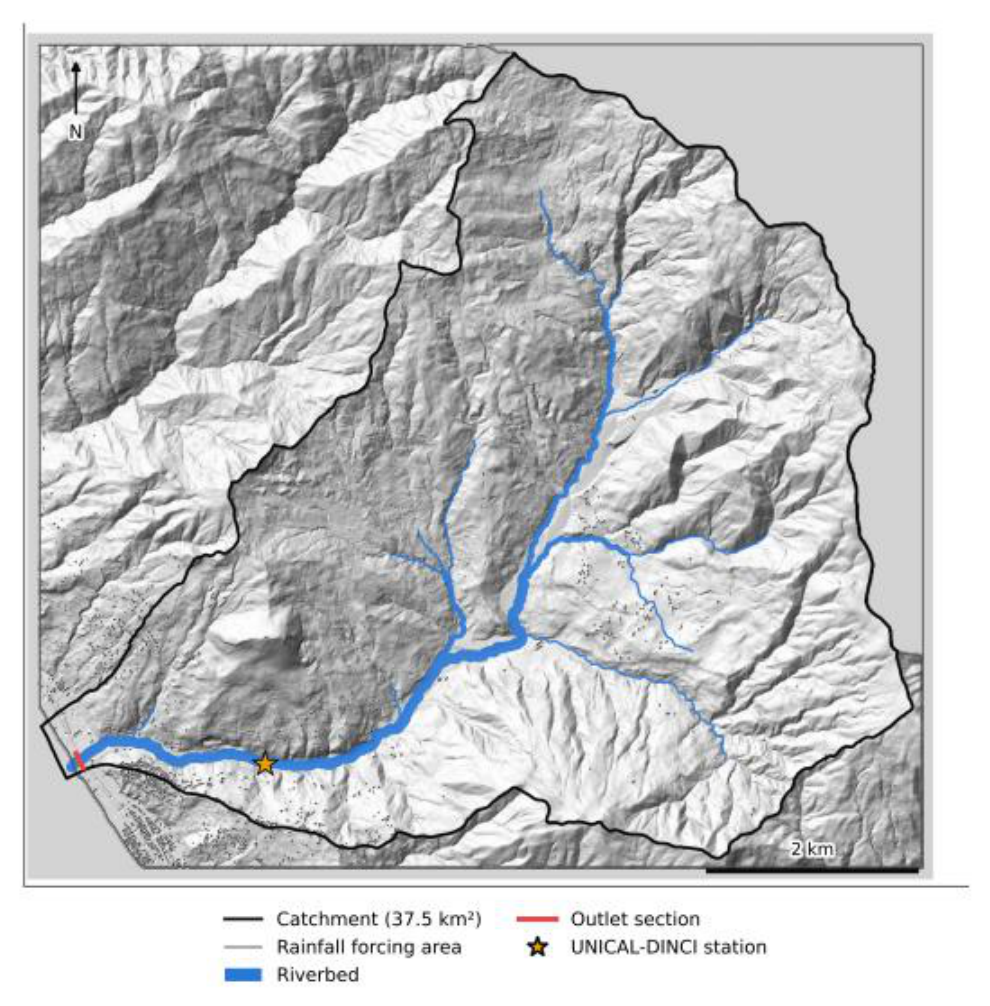
Figure 2.
Rainfall forcing of 12–13 February 2026 (UTC+1). (a) Hourly rainfall at the gauge, radar over 1 km2 around the gauge and radar catchment mean. (b) Cumulative rainfall.
Figure 2.
Rainfall forcing of 12–13 February 2026 (UTC+1). (a) Hourly rainfall at the gauge, radar over 1 km2 around the gauge and radar catchment mean. (b) Cumulative rainfall.
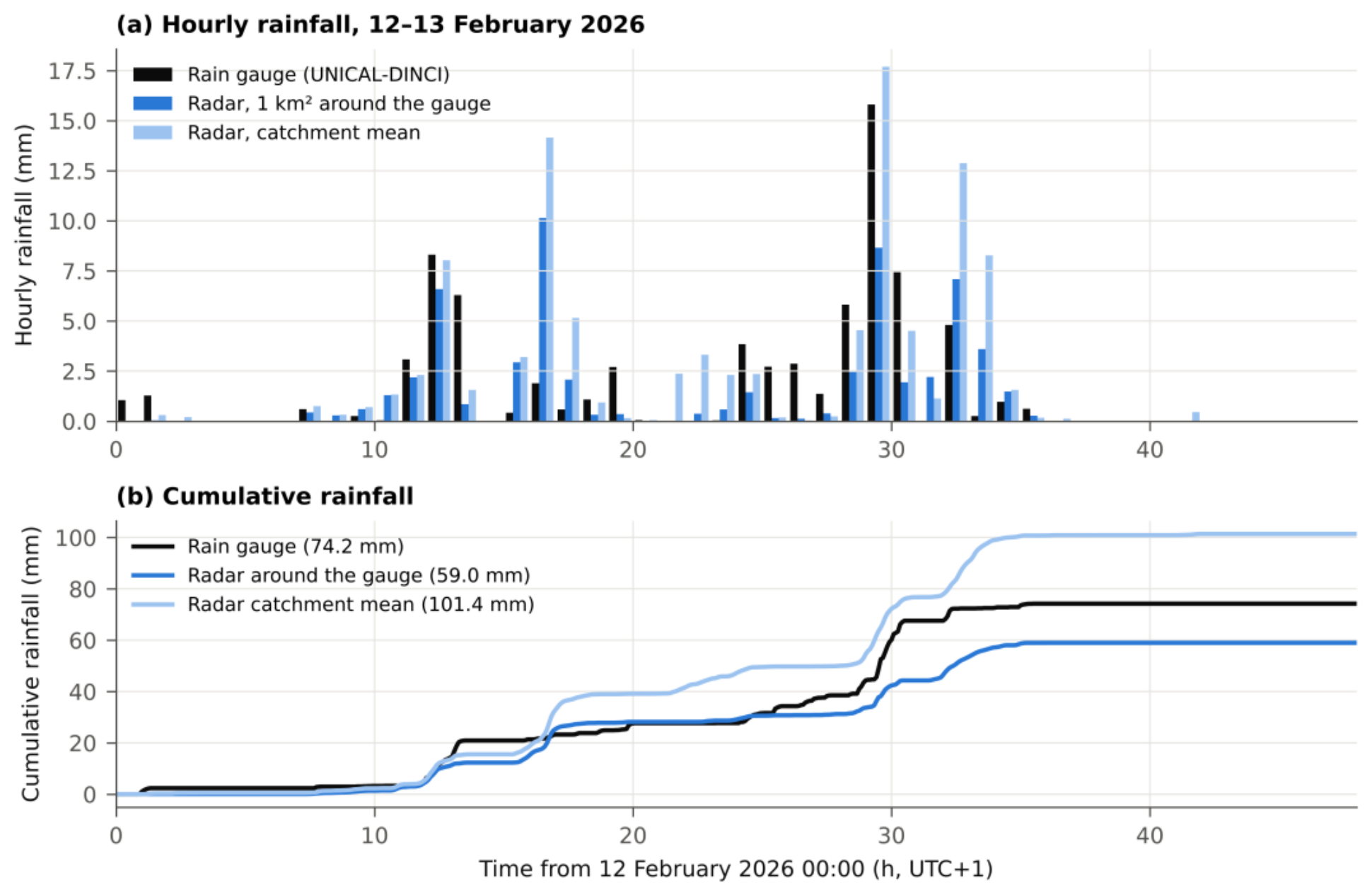
Figure 3.
Loss-model parameters over the rainfall forcing area. (a) CNII from the FOCA map (250 m) over the forcing area. (b) GA texture classes assigned to the lithological units (Table 2).
Figure 3.
Loss-model parameters over the rainfall forcing area. (a) CNII from the FOCA map (250 m) over the forcing area. (b) GA texture classes assigned to the lithological units (Table 2).
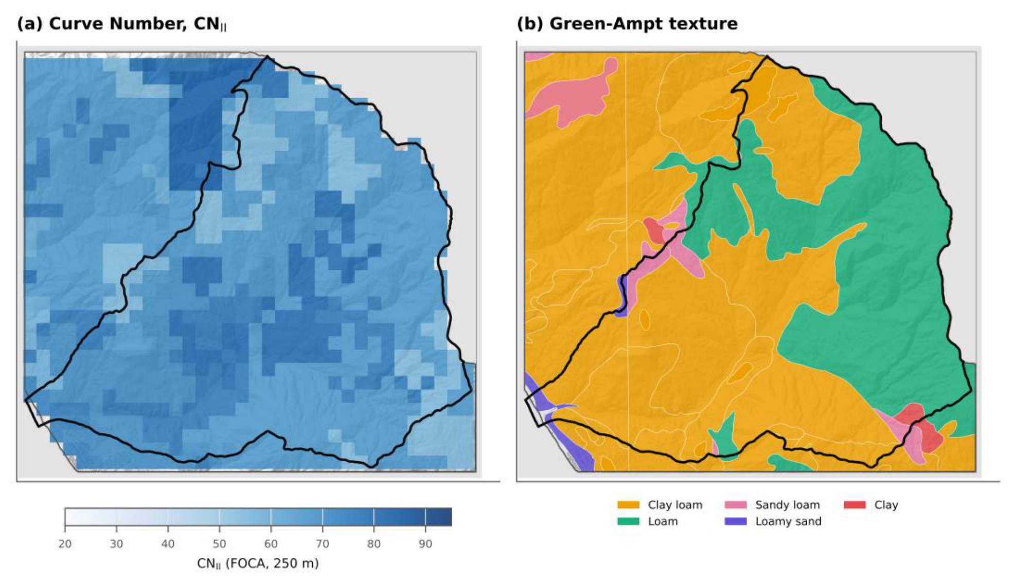
Figure 4.
Water balance over the 59.5 km2 rainfall forcing area, t = 0–48 h (spin-up: t = −48 to 48 h, including 44.4 mm of antecedent rainfall). (a) Radar forcing. (b) Gauge forcing. Run-on infiltration is zero in all SCS-CN runs.
Figure 4.
Water balance over the 59.5 km2 rainfall forcing area, t = 0–48 h (spin-up: t = −48 to 48 h, including 44.4 mm of antecedent rainfall). (a) Radar forcing. (b) Gauge forcing. Run-on infiltration is zero in all SCS-CN runs.
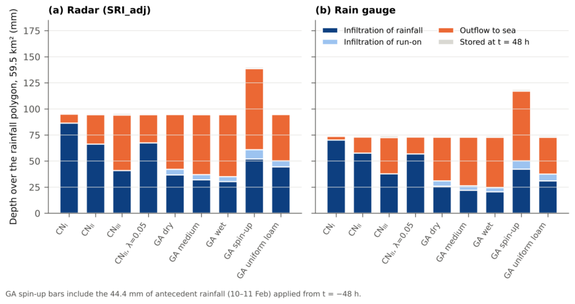
Figure 5.
Hourly rainfall (catchment mean for radar, gauge series for the gauge) and discharge at the outlet. (a) Radar, SCS-CN. (b) Radar, Green-Ampt. (c) Gauge, SCS-CN. (d) Gauge, Green-Ampt.
Figure 5.
Hourly rainfall (catchment mean for radar, gauge series for the gauge) and discharge at the outlet. (a) Radar, SCS-CN. (b) Radar, Green-Ampt. (c) Gauge, SCS-CN. (d) Gauge, Green-Ampt.
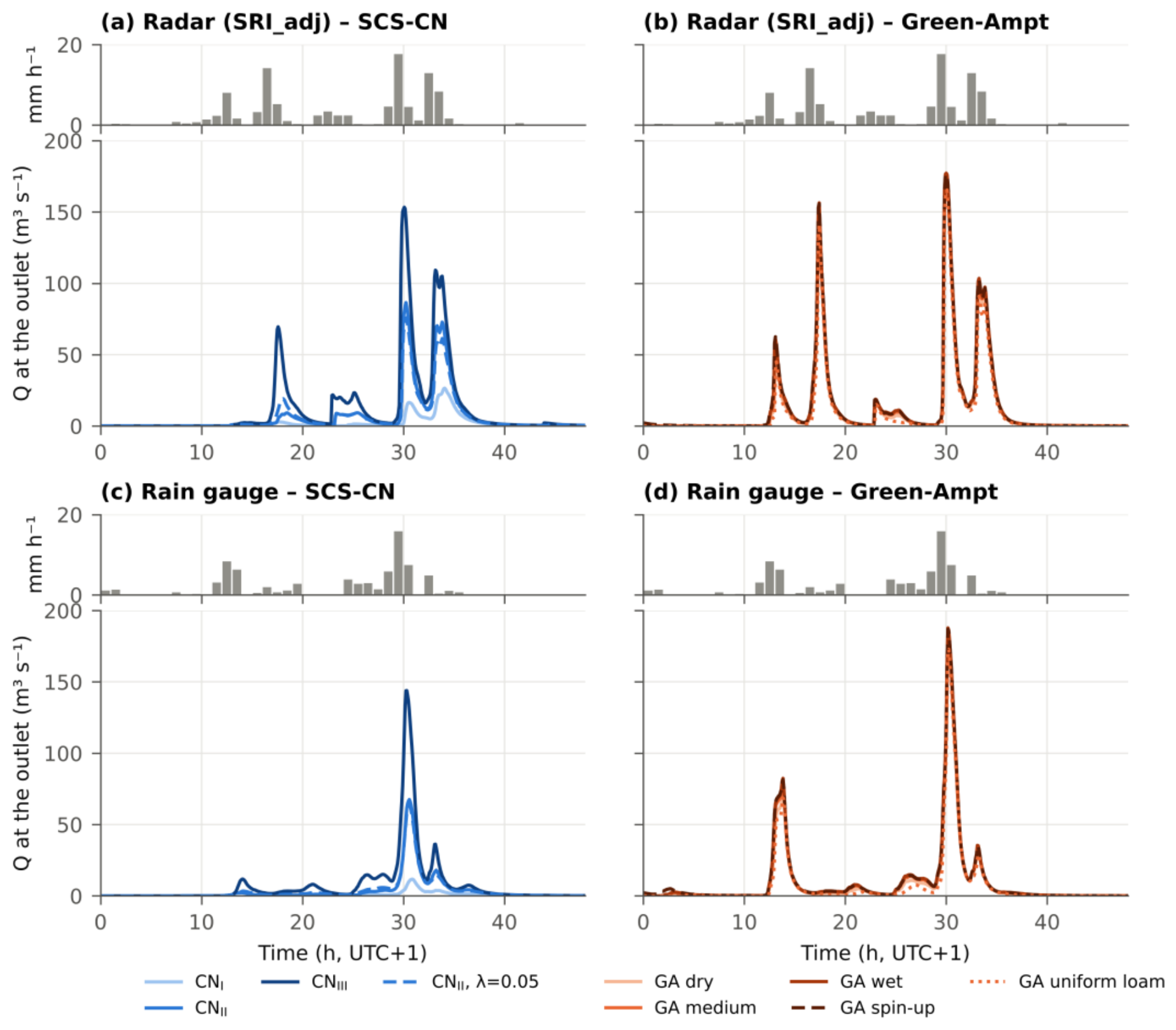
Figure 6.
(a) Peak of the first flow pulse P1 (12 February, 13–14 h) against the main peak at the outlet; the dotted line is 1:1. (b) Main peak against the outlet runoff coefficient. Circles: radar; triangles: gauge. Open symbols: CN II with λ = 0.05 and GA uniform loam.
Figure 6.
(a) Peak of the first flow pulse P1 (12 February, 13–14 h) against the main peak at the outlet; the dotted line is 1:1. (b) Main peak against the outlet runoff coefficient. Circles: radar; triangles: gauge. Open symbols: CN II with λ = 0.05 and GA uniform loam.
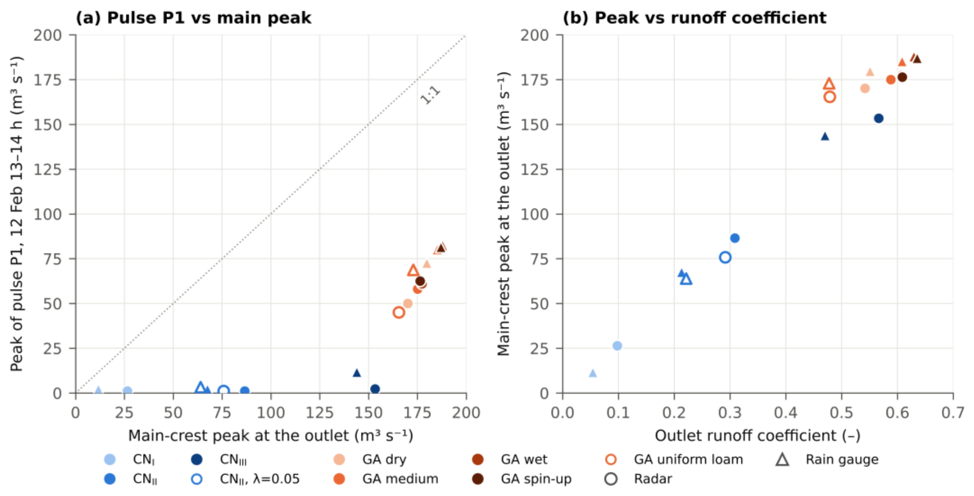
Figure 7.
(a) Point-scale GA infiltration capacity for clay loam (solid) and loam (dotted) in the four initial states, with the 5-min gauge rainfall intensity (log scale). (b) Point-scale cumulative losses: Green-Ampt clay loam (solid) and loam (dotted), and SCS-CN with CN II = 66 under ARC I–III. (c) Cumulative losses over the forcing area in the 2D model, gauge forcing.
Figure 7.
(a) Point-scale GA infiltration capacity for clay loam (solid) and loam (dotted) in the four initial states, with the 5-min gauge rainfall intensity (log scale). (b) Point-scale cumulative losses: Green-Ampt clay loam (solid) and loam (dotted), and SCS-CN with CN II = 66 under ARC I–III. (c) Cumulative losses over the forcing area in the 2D model, gauge forcing.
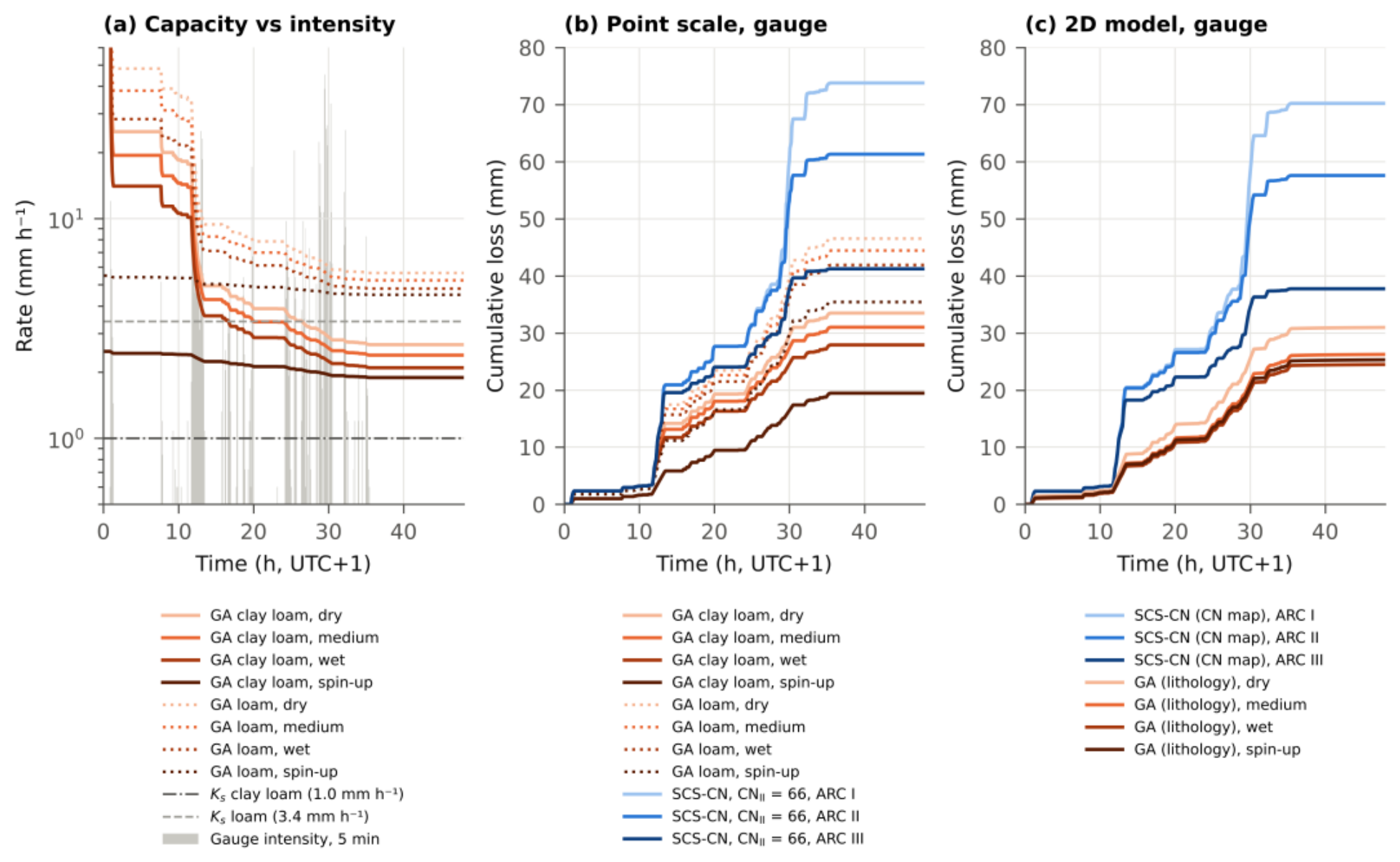
Figure 8.
Velocity at the UNICAL-DINCI station. Observed: surface velocity minus the pre-event median (2.96 m s−1), 5-min values and 35-min moving median. Simulated: depth-averaged velocity of the 10 m cell containing the sensor. (a) Radar forcing. (b) Gauge forcing. Shaded bands: windows P1 and P3.
Figure 8.
Velocity at the UNICAL-DINCI station. Observed: surface velocity minus the pre-event median (2.96 m s−1), 5-min values and 35-min moving median. Simulated: depth-averaged velocity of the 10 m cell containing the sensor. (a) Radar forcing. (b) Gauge forcing. Shaded bands: windows P1 and P3.
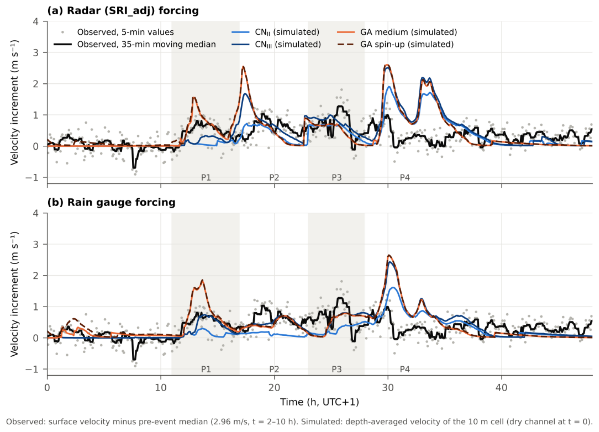
Figure 9.
Difference in maximum depth, radar forcing, over a hillshade of the DTM; thick black line: catchment boundary. (a) GA medium minus CN II. (b) GA spin-up minus CN III. (c, d) Same differences on the coastal plain (dashed box). Cells where both runs stay below 0.05 m, or where the difference is below 0.02 m, are blank. Black lines: outlet and station sections; star: station.
Figure 9.
Difference in maximum depth, radar forcing, over a hillshade of the DTM; thick black line: catchment boundary. (a) GA medium minus CN II. (b) GA spin-up minus CN III. (c, d) Same differences on the coastal plain (dashed box). Cells where both runs stay below 0.05 m, or where the difference is below 0.02 m, are blank. Black lines: outlet and station sections; star: station.
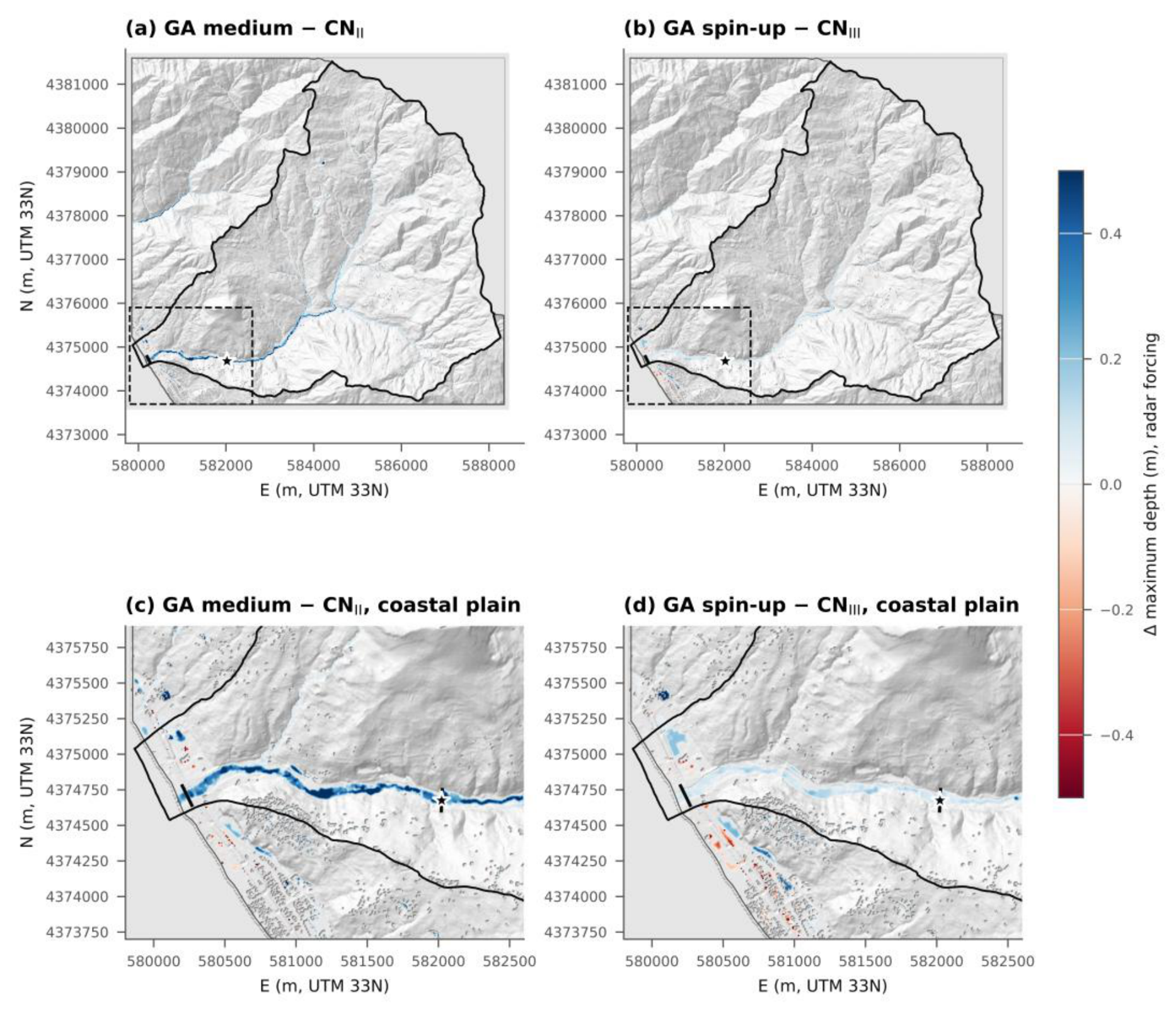

Table 1.
Rainfall and surface velocity at the station by window, 12–13 February 2026.
| Window (t, h) |
Period (UTC+1) | Gauge rainfall (mm) |
Max 5-min intensity (mm h−1) | Median velocity (m s−1) |
Max of 35-min median (m s−1) |
|---|---|---|---|---|---|
| 0–11 | 12 Feb 00:00–11:00 | 3.2 | 12.0 | 2.99 | 3.32 at 01:50 |
| 11–17 (P1) | 12 Feb 11:00–17:00 | 20.0 | 25.0 | 3.40 | 3.77 at 13:10 |
| 17–23 (P2) | 12 Feb 17:00–23:00 | 4.4 | 17.2 | 3.49 | 3.99 at 18:55 |
| 23–28 (P3) | 12 Feb 23:00 – 13 Feb 04:00 | 10.9 | 20.4 | 3.63 | 4.24 at 01:40 |
| 28–35 (P4) | 13 Feb 04:00–11:00 | 35.1 | 45.1 | 3.24 | 3.95 at 05:55 |
| 35–48 | 13 Feb 11:00–24:00 | 0.6 | 2.9 | 3.28 | 3.55 at 13:40 |
| Lithology (domain area, km2) |
Texture | ψ (mm) | Ks (mm h−1) | θe |
θi dry / medium / wet |
|---|---|---|---|---|---|
| Phyllites and micaschists (37.0); dolomites (2.5); marbles (1.7); evaporites (0.4); basic lavas (0.2) | Clay loam | 208.8 | 1.0 | 0.309 | 0.042 / 0.103 / 0.163 |
| Gneiss (24.4) | Loam | 88.9 | 3.4 | 0.434 | 0.088 / 0.165 / 0.241 |
| Granitoids (1.5); sandstones (0.7); mixed-grain terraces (0.4); travertine (0.1) | Sandy loam | 110.1 | 10.9 | 0.412 | 0.054 / 0.110 / 0.166 |
| Gravelly alluvium and marine terraces (0.7) | Loamy sand | 61.3 | 29.9 | 0.401 | 0.019 / 0.054 / 0.089 |
| Pelitic-arenaceous units with gypsum (0.5) | Clay | 316.3 | 0.3 | 0.385 | 0.182 / 0.244 / 0.306 |
| Beach | Sand | 49.5 | 117.8 | 0.417 | 0.35 (all scenarios) |
Table 3.
Scenario matrix. Each scenario was run with radar (R) and rain-gauge (G) forcing; all runs start at t = 0 h with a dry domain, except GA spin-up (t = −48 h).
Table 3.
Scenario matrix. Each scenario was run with radar (R) and rain-gauge (G) forcing; all runs start at t = 0 h with a dry domain, except GA spin-up (t = −48 h).
| Scenario | Loss model | Parameters and initial state | Role |
|---|---|---|---|
| CN I | SCS-CN | FOCA CN, ARC I, λ = 0.2 | lower bound of SCS-CN runoff |
| CN II | SCS-CN | FOCA CN, ARC II, λ = 0.2 | standard practice |
| CN III | SCS-CN | FOCA CN, ARC III, λ = 0.2 | ARC implied by antecedent rainfall |
| CN II, λ = 0.05 | SCS-CN | converted CN II, λ = 0.05 | initial abstraction ratio |
| GA dry | Green-Ampt | lithology-based, θi at wilting point | driest initial state |
| GA medium | Green-Ampt | lithology-based, medium θi | reference Green-Ampt |
| GA wet | Green-Ampt | lithology-based, θi at field capacity | wettest prescribed state |
| GA spin-up | Green-Ampt | lithology-based, medium θi on 10 Feb, then 44.36 mm of antecedent rainfall | rainfall-driven initial state |
| GA uniform loam | Green-Ampt | uniform loam (LUCAS), Rawls et al. [10] | texture source and spatial distribution |
Table 4.
Hydrological indicators at the outlet. Times on 13 February (UTC+1); RP1 and RP2 = peak of the first flow pulse and of the radar pulse at 16–17 h, as fractions of the main peak; infiltration over the forcing area; flooded area outside the riverbed.
Table 4.
Hydrological indicators at the outlet. Times on 13 February (UTC+1); RP1 and RP2 = peak of the first flow pulse and of the radar pulse at 16–17 h, as fractions of the main peak; infiltration over the forcing area; flooded area outside the riverbed.
| Forcing | Scenario | Qp (m3 s−1) | Time of Qp | RP1 | RP2 | Volume (106 m3) | C | Infiltration (mm) |
of which run-on (mm) | Area hmax ≥ 0.1 m outside bed (km2) |
|---|---|---|---|---|---|---|---|---|---|---|
| R | CN I | 26.5 | 10:05 | 0.04 | 0.11 | 0.37 | 0.10 | 86.3 | 0 | 0.21 |
| R | CN II | 86.5 | 06:15 | 0.01 | 0.11 | 1.17 | 0.31 | 66.3 | 0 | 0.43 |
| R | CN III | 153.4 | 06:05 | 0.02 | 0.45 | 2.15 | 0.57 | 41.0 | 0 | 0.66 |
| R | CN II, λ = 0.05 | 75.8 | 06:15 | 0.01 | 0.25 | 1.11 | 0.29 | 67.5 | 0 | 0.40 |
| R | GA dry | 170.1 | 06:00 | 0.29 | 0.86 | 2.06 | 0.54 | 42.1 | 5.4 | 0.70 |
| R | GA medium | 175.0 | 06:00 | 0.33 | 0.87 | 2.24 | 0.59 | 37.1 | 5.0 | 0.72 |
| R | GA wet | 177.3 | 06:00 | 0.34 | 0.88 | 2.31 | 0.61 | 35.0 | 4.7 | 0.73 |
| R | GA spin-up | 176.4 | 06:00 | 0.35 | 0.88 | 2.31 | 0.61 | 36.0 (+24.9 before t = 0) |
8.9 | 0.76 |
| R | GA uniform loam | 165.4 | 06:05 | 0.27 | 0.85 | 1.82 | 0.48 | 50.3 | 5.9 | 0.70 |
| G | CN I | 11.7 | 06:55 | 0.19 | – | 0.15 | 0.05 | 70.2 | 0 | 0.14 |
| G | CN II | 67.5 | 06:35 | 0.03 | – | 0.59 | 0.21 | 57.6 | 0 | 0.37 |
| G | CN III | 143.9 | 06:20 | 0.08 | – | 1.31 | 0.47 | 37.8 | 0 | 0.66 |
| G | CN II, λ = 0.05 | 64.0 | 06:30 | 0.05 | – | 0.62 | 0.22 | 56.9 | 0 | 0.37 |
| G | GA dry | 179.7 | 06:10 | 0.40 | – | 1.53 | 0.55 | 31.0 | 5.1 | 0.74 |
| G | GA medium | 185.2 | 06:10 | 0.43 | – | 1.69 | 0.61 | 26.3 | 4.3 | 0.77 |
| G | GA wet | 187.8 | 06:10 | 0.44 | – | 1.75 | 0.63 | 24.5 | 3.9 | 0.78 |
| G | GA spin-up | 187.0 | 06:10 | 0.44 | – | 1.77 | 0.64 | 25.3 (+24.9 before t = 0) |
8.0 | 0.80 |
| G | GA uniform loam | 172.9 | 06:15 | 0.40 | – | 1.33 | 0.48 | 37.6 | 6.6 | 0.76 |
Table 5.
Velocity indicators at the station: Δt = simulated minus observed time of the maximum in windows P1 and P4 (min); P1/P3 and P1/P4 = ratios of velocity increments (observed 0.63 and 0.82); r = Pearson correlation for t = 6–40 h.
Table 5.
Velocity indicators at the station: Δt = simulated minus observed time of the maximum in windows P1 and P4 (min); P1/P3 and P1/P4 = ratios of velocity increments (observed 0.63 and 0.82); r = Pearson correlation for t = 6–40 h.
| Forcing | Scenario | Δt P1 | Δt P4 | P1/P3 | P1/P4 | r |
|---|---|---|---|---|---|---|
| R | CN II | no response | +10 | 0.30 | 0.11 | 0.14 |
| R | CN III | no response | +5 | 0.82 | 0.33 | 0.19 |
| R | GA medium | −15 | 0 | 1.87 | 0.60 | 0.19 |
| R | GA spin-up | −15 | 0 | 1.91 | 0.62 | 0.18 |
| G | CN II | +30 | +30 | 0.58 | 0.19 | 0.07 |
| G | CN III | +40 | +15 | 0.92 | 0.30 | 0.28 |
| G | GA medium | +30 | +10 | 2.33 | 0.69 | 0.30 |
| G | GA spin-up | +30 | +10 | 2.34 | 0.70 | 0.29 |
Table 6.
Sensitivity runs, radar forcing. Reference runs in the first row of each group.
| Run | Qp (m3 s−1) | Time of Qp (13 Feb) | RP1 | RP2 | Volume (106 m3) | Infiltration (mm) | Max velocity at station (m s−1) |
Area hmax ≥ 0.1 m outside bed (km2) |
|---|---|---|---|---|---|---|---|---|
| CN III | 153.4 | 06:05 | 0.02 | 0.45 | 2.15 | 41.0 | 2.51 | 0.66 |
| CN III, n × 0.8 | 155.5 | 06:05 | 0.02 | 0.48 | 2.16 | 40.9 | 2.80 | 0.60 |
| CN III, n × 1.2 | 151.3 | 06:10 | 0.01 | 0.43 | 2.15 | 40.9 | 2.27 | 0.72 |
| GA medium | 175.0 | 06:00 | 0.33 | 0.87 | 2.24 | 37.1 | 2.61 | 0.72 |
| GA medium, n × 0.8 | 179.1 | 05:50 | 0.36 | 0.92 | 2.25 | 36.8 | 2.89 | 0.65 |
| GA medium, n × 1.2 | 172.5 | 06:05 | 0.30 | 0.83 | 2.23 | 37.3 | 2.38 | 0.78 |
| GA medium, Ks × 3 | 126.4 | 06:05 | 0.09 | 0.68 | 1.11 | 65.5 | 2.32 | 0.48 |
| GA medium, Ks × 10 | 41.0 | 06:20 | 0.03 | 0.25 | 0.23 | 89.6 | 1.35 | 0.20 |
Table 7.
Spread of peak discharge, runoff volume at the outlet and area with hmax ≥ 0.1 m outside the riverbed, by model and parameter group (R = radar, G = gauge).
Table 7.
Spread of peak discharge, runoff volume at the outlet and area with hmax ≥ 0.1 m outside the riverbed, by model and parameter group (R = radar, G = gauge).
| Model | Parameter varied | Forcing | Qp (m3 s−1) | Volume (106 m3) | Area (km2) |
|---|---|---|---|---|---|
| SCS-CN | ARC I–III, λ | R | 26.5–153.4 | 0.37–2.15 | 0.21–0.66 |
| SCS-CN | ARC I–III, λ | G | 11.7–143.9 | 0.15–1.31 | 0.14–0.66 |
| Green-Ampt |
θi, spin-up, texture source |
R | 165.4–177.3 | 1.82–2.31 | 0.70–0.76 |
| Green-Ampt |
θi, spin-up, texture source |
G | 172.9–187.8 | 1.33–1.77 | 0.74–0.80 |
| Green-Ampt | Ks × 1–10 | R | 41.0–175.0 | 0.23–2.24 | 0.20–0.72 |
| SCS-CN (ARC III) | Manning’s n ± 20% | R | 151.3–155.5 | 2.15–2.16 | 0.60–0.72 |
| Green-Ampt (medium) |
Manning’s n ± 20% | R | 172.5–179.1 | 2.23–2.25 | 0.65–0.78 |
Disclaimer/Publisher’s Note: The statements, opinions and data contained in all publications are solely those of the individual author(s) and contributor(s) and not of MDPI and/or the editor(s). MDPI and/or the editor(s) disclaim responsibility for any injury to people or property resulting from any ideas, methods, instructions or products referred to in the content. |
© 2026 by the authors. Licensee MDPI, Basel, Switzerland. This article is an open access article distributed under the terms and conditions of the Creative Commons Attribution (CC BY) license (http://creativecommons.org/licenses/by/4.0/).
Copyright: This open access article is published under a Creative Commons CC BY 4.0 license, which permit the free download, distribution, and reuse, provided that the author and preprint are cited in any reuse.