

Submitted:
13 November 2026
Posted:
16 November 2026
You are already at the latest version
Abstract
The design of a stepped hydrostatic thrust bearing with an opposed lubrication system is considered. A mechanism for increasing the bearing capacity through the use of an opposed system is described. A mathematical model of the static and dynamic state of the structure is formulated. Methods for calculating the bearing capacity, compliance, and lubricant flow rate have been developed. The calculations are performed in dimensionless form. The use of an opposed system in combination with a stepped axial gap configuration allows virtually maximum bearing capacity values, for which the utilization of the bearing surface area can reach 95% or more, whereas in a thrust bearing with an opposed system and a flat gap, this value is approximately 75%, and in a conventional thrust bearing, it is approximately 50%. Thus, the use of an opposed system and a step allows for a significant increase in the bearing capacity, which is 20–30% greater than that of a thrust bearing with an opposed system and a flat gap and almost twice that of a conventional thrust bearing. In this case, compliance can be reduced by a factor of 2–3, and the flow rate can be reduced by at least an order of magnitude. A study of dynamic quality criteria has shown that there are optimal values for the pressure settings χ and ς in terms of response speed and stability margin, as well as the "compression number" σ, which determines the optimal damping of the lubricant film.
Keywords:
hydrostatic stepped thrust bearing
; opposite lubrication system
; bearing capacity
; compliance
; lubricant flow rate
; dynamic quality
1. Introduction
Hydrostatic plain bearings are used in various technical fields, particularly in mechanical engineering [1,2]. These designs ensure high positioning accuracy, which is critical for precision equipment, such as turning, milling, and grinding machines, coordinate measuring machines, and optical telescopes [3,4]. The low coefficient of friction helps reduce the energy consumption of such designs. Their main advantage over other types of bearings is that a gap of liquid lubricant—oil or water—is located between the moving surfaces, eliminating contact between them and significantly reducing friction. As a result, the service life of bearings is significantly increased [5,6]. A thin gap of liquid helps dissipate heat generated during operation, thereby preventing overheating of the bearing and the machine. An example is bearings that use cold water as a lubricant [7,8]. This ensures a constant operating temperature, which is important for ensuring the stability of the equipment’s operating characteristics and the durability of the bearing.
Moreover, in the designs of traditional hydrostatic bearings, especially in thrust bearings, the systems for delivering lubricant to the supporting lubricant gap are such that the areas of their supporting surfaces are not used effectively. Recently, hydrostatic bearing designs and studies have shown that replacing the traditional lubrication supply system with an alternative system can achieve a significant increase in the bearing capacity and a decrease in compliance (increased stiffness) [9,10]. Unlike rolling bearings, hydrostatic bearings require energy [11,12]. Research has shown that the use of an opposite lubrication system allows for a several-fold reduction in the fluid flow rate and, consequently, a reduction in the energy costs for pumping it through the bearing [9,10].
In a thrust bearing with an opposed lubrication system, the fluid flow moves from the periphery to the center, allowing for more efficient use of the bearing surface area and the lubricant pressure acting on them, significantly improving the performance of the thrust bearing. In this case, the term "opposed lubrication system" indicates that in this thrust bearing, the direction of lubricant flow is opposite to that of traditional thrust bearing designs with an external pressure source, in which the fluid flow moves from the center to the periphery.
The first paper on bearings with an opposed lubrication system presented a conceptual model, which was difficult to implement in practice due to technological complexities [16]. This paper proposes a technologically advanced design that is readily implemented in practice. This paper examines a stepped hydrostatic thrust bearing, which is consistent with the development of the opposed lubrication system. Compared with the thrust bearing [16], the proposed design includes a step in the bearing gap at the fluid outlet. This step significantly limits the lubricant flow rate, thereby further increasing the bearing capacity and reducing the compliance and lubricant flow rate, which should result in more efficient energy consumption by the thrust bearing.
2. Description of the Mechanism for Increasing the Bearing Capacity
To explain the physical mechanism of increasing the load-bearing capacity by changing the direction of lubricant flow, we will conduct comparative calculations using the example of a design with direct and opposite directions of fluid flow in the gap.
Figure 1 shows a diagram of an annular lubrication gap with pressures p1 and p0 at its edges. For p1 > p0, we obtain direct lubricant flow; for p1 < p0, we obtain the opposite.
The pressure function p = p (r) in the carrier gap obeys the boundary value problem for the Reynolds equation [13]:
The solution to problem (1) is the function
Let us introduce the dimensionless radius R1 = r1 / r0. Using (2), we find the bearing capacity of the lubricating film.
Let us assume, for example, that r0 = 0.025 m and R1 = 0.5. For direct flow, we take, for example, p0 = 1 MPa and p1 = 3 MPa. The calculation via formula (3) gives w = 2615 N. For an opposite flow with p0 = 3 MPa and p1 = 1 MPa, w = 3275 N. The ratio of these values is 3275/2615 = 1.25. Thus, changing the direction of the lubricant flow from straight to opposite in this case results in a 1.25-fold increase in the bearing capacity.
Let us introduce the “coefficient of utilization of the supporting surface area” Cw. In the ideal case, when the greatest pressure acts over the entire area, pmax = max(p0,p1)the coefficient Cw = 100%. In the absence of pressure, Cw = 0%. In our case, For direct flow, Cw = 100.w/wl = 2615/4417*100 = 59%. For reverse flow, Cw = 100.w/wl = 3275/4417 = 74%. Thus, in the first case, the bearing area is used by only 59%, whereas in the second case, it is significantly better, by 74%. As seen from the calculated data, even for an opposite system, there remains a certain opportunity for further increasing the bearing capacity with an unchanged bearing surface area.
Notably, the opposed system is characterized by small internal radii, down to R1 = 0.05. In this case, the advantages of such a system will be even more significant, as the bearing area will be utilized by Cw = 89%, and the bearing capacity of the thrust bearing will increase accordingly.
3. Description of the Thrust Bearing and Its Operating Principle
The design scheme of a stepped thrust bearing with an opposite lubrication system is shown in Figure 2.
The design consists of a fixed body 1 and a heel 2 of mass m. Lubricant under external pressure ps enters through opening 3 into the inlet of a radial gap 4 of thickness hr. In gap 4, the flow bifurcates. One part flows under pressure pc into an axial gap 5 of thickness h, and the other flows to the drain under pressure pa, thereby ensuring the operability of the thrust bearing. After overcoming the hydraulic resistance of gap 5, the lubricant under pressure pm enters gap 6 with a thickness hm of radius r1. From gap 6, it flows out to the drain through cylindrical opening 7 of radius r2.
When gap 5 decreases, the load f on the thrust bearing increases, creating increased resistance to fluid outflow. At the same time, Gap 6 decreases, creating increased hydraulic resistance to fluid outflow, resulting in a significantly greater increase in pressure than if the step is absent. This should result in increased load-bearing capacity, reduced compliance and lubricant flow rate, and, consequently, reduced thrust bearing energy consumption.
4. Mathematical Model of the Motion of the Thrust Bearing
For calculations, we use an isothermal model, according to which the temperature in the thrust bearing and, consequently, the dynamic viscosity of the lubricant are constant values [14].
The mathematical model of the motion of the thrust bearing includes an equation for the balance of forces acting on thrust bearing 2 and two equations for the balance of volumetric flow rates through the radial and axial gaps.
w − fin = f,
qr − qh0 = 0,
qh1 − qm = 0.
Here,
– bearing capacity of the thrust bearing [15],
– the force of inertia of the heel, f – external load,
– lubricant flow rate at the entrance to gap 5 [15], where µ is the dynamic viscosity of the lubricant,
– flow rate at the outlet of gap 5,
– flow rate at the entrance of gap 6,
– lubricant flow through radial gap 4 in the direction of radial gap 5 [16].
The pressure function p = p (r, t) in bearing gap 5 of thickness h obeys the boundary value problem for the Reynolds equation [14]:
The pressure function p = p (r, t) in a gap 6 of thickness h m obeys the boundary value problem
The pressure function p = p (z) in a gap 4 of constant thickness hr is the solution of the boundary value problem for the Reynolds equation [16]
where l1 is the length of the radial channel in the direction of gap 5.
Similarly, for the pressure in gap 4, which corresponds to the drain, we have a boundary value problem
where l2 is the length of this part of the radial channel.
5. The Mathematical Model is Reduced to a Dimensionless Form
The calculations are performed via dimensionless quantities. For this purpose, we take the radius r0 as the scale of linear dimensions; for gaps, h = h0, which is adjusted to withstand the calculated load f0; the supply pressure ps for pressures; and πr02 ps for forces, πh03 ps/(6 µ) for volumetric lubricant flow rates.
The dimensionless mathematical model of the static state of the thrust bearing, taking into account (4) – (6), after being reduced to dimensionless form, is written in the form
W − Fin = F,
Qr − Qh0 = 0,
Qh1 − Qm = 0.
The dimensionless boundary value problem (13) for the region R1 ≤ R ≤ 1will take the form
where Pc and Pm are dimensionless pressures at the edges of gap 5,
– the so-called “compression number” [17], t0 – the scale of the current time, and τ = t/t0 – the dimensionless current time.
Similarly, the dimensionless boundary value problem (14) for the region R2 ≤ R ≤ R1will take the form
The solutions to boundary value problems (20) and (22) are functions (23) and (24), respectively:
The dimensionless boundary value problem (13) takes the form
where L1 = l1 / r0 is the dimensionless length of the corresponding part of radial channel 4.
The solution to the boundary value problem (25) is the function
P(Z,τ) = 1 + (Pс − 1)Z/L1.
The dimensionless boundary value problem (14) has the form
where L2 = l2 / r0 is the dimensionless length of the corresponding part of radial channel 4.
The solution to problem (27) is the function
P(Z) = 1 − Z/L2.
The bearing capacity of the thrust bearing is equal to
where
Substituting (30) and (31) into (29), we obtain a formula for the dynamic bearing capacity
where In accordance with (8), the formula for the dimensionless inertial force of heel 2 takes the form
where is the dimensionless mass of heel 2.
W = W1 + W2,
We find the scale of the current time from the condition of the unit mass of the heel M = 1. In this case, we obtainAccording to (12), the formula for the dimensionless lubricant flow rate in the radial gap in the direction of axial gap 5, taking into account (26), takes the form
where
The corresponding (9) formula for the flow rate at the entrance to the axial gap, taking into account (23), takes the form
where
Similarly, using (10) and (23), we obtain a formula for the lubricant flow rate at the outlet of gap 5:
where
The formula for the flow rate at the entrance to gap 6 according to (11) and (24) takes the form
where
Substituting (32), (34), (35) – (37) into (17) – (19), we obtain a system of equations that form a mathematical model of the dynamics of the thrust bearing
where Λ = λ/h 0 is the dimensionless height of the step and where λ is its dimensional height.
H − Hm=Δ,
6. Static Characteristics of the Bearing and Method of Calculation
In the absence of oscillations, the stationary model of the thrust bearing is simplified and takes the form
AwcPc + AwmPm = F,
Ar(1 − Pc) − AhH3(Pc − Pm) = 0,
H − Hm−Δ=0.
In the calculations, we take the values of the radii R1 = 0.20 and R2 = 0.05. In addition, we use the pressure setting parameters χ ∈ [0,1] and ς ∈ [0,1], corresponding to the design load F = F0 and a gap H = 1
Pc0 = χ,Pm0 = ςPc0.
Considering (46), we find the design flow rate, the flow rate parameter in the radial gap, the gap in the step area and its height
Since Hm0 < 1,, using equation (44) for the design mode, we obtain ςmin < ς < 1,, where ςmin = [1 − ln(R1)]/ln(R2).For the given values of the radii, this corresponds to ςmin = 0.462.
When constructing steady-state curves, it is convenient to use pressure as a parameter Pc ∈ [0,1]. In this case, the gaps H and H m, as well as the pressure Pm, remain unknown. Using (44), we find
Substituting (47) into (43) yields a nonlinear equation with only one unknown pressure Pm. Its solution for each value of the parameter Pc was found via the numerical bisection method [18]. For this purpose, obvious conditions were used 0 ≤ Pm ≤ Pc.. In the process of solving this equation, the values of the gaps H and Hm were simultaneously determined.
Next, we find the bearing capacity via formula (42) and the total flow rate via formula
Qs = Qr1 + Qr2 = Ar(2 − Pc).
To determine the compliance K of the thrust bearing, by differentiating equations (38) and (41) with respect to the pressure Pc, we obtain the following formula:
where
K = −H′/W′,
These formulas were then used to calculate the characteristics of the thrust bearing.
7. Static Characteristics of the Bearing
Figure 3 shows the graphs of the dependence of the gap Hm in the step area on the load F for χ = 0.6 and different values of the coefficient ς.
Two circumstances are noteworthy. The slopes of the curves change noticeably as the parameter ς increases. As ς increases, the curves become steeper in the low-load range, whereas at medium and high loads, the relationships, by contrast, exhibit a flatter profile.
This observation indicates that, excluding low loads, the compliance of a thrust bearing decreases (its stiffness increases) as ς increases within the range of moderate loads.
The second circumstance is that, as seen from the graphs, with an increase in ς, the range of perceived loads expands. Thus, at ς = 0.498, for which the step height is minimal, the thrust bearing is capable of withstanding a maximum load of up to 0.87. Theoretically, the maximum value of the coefficient Cw= 100%. In this case, the injection pressure ps should act over the entire area of the supporting surface of radius r2 ≤ r ≤ r0. Thus, Taking into account the scale of the forces, the corresponding dimensionless quantity for the radius R2 = 0.05. At ς = 0.498, Cw = Wmax/Wl = 100% = 87% of the supporting area is used. At ς = 0.606, it is already used by Cw = 92%, at ς = 0.713 by 95%, at ς = 0.821 by Cw = 97% and at ς = 0.928 by Cw = 98%. Note that in a conventional thrust bearing with a direct lubrication supply system, approximately Cw = 50% of the area is used [19]. In a thrust bearing with a standard gap and an opposed system, this value is approximately Cw = 75%. If such a thrust bearing is stepped, its load-bearing capacity can be almost doubled compared with that of a standard thrust bearing.
In practice, one can employ a stage corresponding to ς = 0.606. This yields a very high value of Cw = 95% at a relatively small stage height of Δ = δ/h0 = 0.18. A design with these parameters is well suited for manufacturing and can accommodate high, moderate, and low loads alike while posing virtually no obstacle to minimizing the primary gap h. For such a loading regime, ideal thrust-bearing dynamics can be achieved by selecting an optimal value for the “compression number” σ (Figure 10).
Thus, the use of an opposite lubrication system in combination with a stepped axial gap design allows for the achievement of virtually maximum thrust bearing capacity, which is impossible to exceed even theoretically. This is the main conclusion reached on the basis of a study of the static characteristics of the thrust bearing under study.
Figure 4 shows the graphs of the dependence of the thrust bearing compliance K on the load F for χ = 0.6 and different values of the coefficient ς.
Clearly, with increasing ς, the compliance K decreases significantly. Thus, at ς = 0.498, for which the step has a minimum height, the minimum compliance K = 1.55. Furthermore, with increasing ς, it decreases to K = 0.57 at ς = 0.928, that is, by almost three times.
In [16], it was shown that, compared with a conventional thrust bearing, an opposed system with a flat axial gap offers no advantages in compliance. However, as we can see, it is possible to significantly improve the characteristics, reducing compliance several times in a thrust bearing with an opposed system, by using a stepped axial gap.
Figure 5 shows the graphs of the dependence of the total lubricant flow rate Qs on the load F for χ = 0.6 and different values of the coefficient ς.
It is evident that with increasing values of the parameter ς, the flow rate decreases significantly. Thus, at the highest value of ς = 0.968, when the step height Δ = 0.594, compared with ς = 0.498 (step height Δ = 0.046), for example, at F = 0.8, the corresponding flow rate figures are Qs1 = 0.50 and Qs2 = 0.08. Thus, the use of a step alone allows for a reduction in the lubricant flow rate and, with its energy consumption, by approximately Qs1 / Qs2 = 6 times.
In [16], it was shown that the opposed system allows for a reduction in the fluid flow rate by approximately 2–3 times. Consequently, compared with a conventional thrust bearing, the flow rate of a thrust bearing with a step and opposed system is 10 times lower or greater. The energy consumption of the structure is also reduced by the same factor.
Comparative studies of the static characteristics of the thrust bearings have shown the exceptionally high efficiency of using the stage in combination with the opposite lubrication system, which allows practically achieving the maximum efficiency of using the bearing surface area, reducing compliance by 2–3 times and reducing the flow rate and, consequently, the energy consumption of the thrust bearing by at least 10 times.
However, it should be noted that increasing the step height, for example, to Δ = 0.8, and decreasing the step radius to R1 = 0.10 are still possible. In this case, the support area utilization factor becomes practically limiting (Cw = 99.5%), and the flow rate decreases even further so that the thrust bearing becomes practically flow rate-free and the compliance approaches zero (infinite stiffness). Improving its characteristics as a passive support is no longer possible, even theoretically. If necessary, the compliance of the structure can be reduced to negative values [20]. However, this can only be realized in a support containing an active element [21,22,23].
To study the capabilities of the opposed heel plate, it is necessary to confirm that, in addition to the advantages mentioned above, it has acceptable dynamic performance indicators.
8. Linear Model of Bearing Dynamics
An increasing load is known to be a factor in the stabilization of hydrostatic bearings [24,25]. Consequently, their poorest performance will occur with small oscillations of the moving element caused by small disturbances of the external force. Therefore, to determine the quality of the thrust bearing's dynamics, it is sufficient to examine its response to small disturbances of the external load, since its performance will not deteriorate with moderate and large oscillation amplitudes.
8.1. Derivation of the Characteristic Equation and the Compliance Transform
Let us consider the dynamic model (38) – (41) and represent its nonstationary functions in the form
where ΔH(τ),ΔPc(τ),ΔPm(τ),ΔHm(τ),ΔF(τ) are small dynamic deviations of functions from the corresponding stationary valuesH,Pc,ΔPm,Hm,F.
|ΔH|<<H, |ΔPc|<<Pc, |ΔPm|<<Pm, |ΔHm|<<Hm,|ΔF|<<F,
Substituting (49) into (38) – (40) and considering that, according to (41) ΔH=ΔHm,after linearization, we obtain a mathematical model of the dynamics of the thrust bearing in small deviations
where
By applying the Laplace integral transform [26] to (50) – (52), we obtain the corresponding system of equations in the Laplace transform:
where represents the transformants of the corresponding deviations and where s is the Laplace transform variable.
Let us write (53) – (55) in matrix form
The determinant of the matrix (56) is the characteristic polynomial of the dynamic system
where
a0 + σa1s + a1s2 = 0,
Having solved (56), we find the transfer function of the transform of the dynamic compliance of the thrust bearing
Obviously, the static compliance K(0) = b0/a0 exactly corresponds to (48).
9. Quality of the Bearing Dynamics
To evaluate the quality of the thrust bearing dynamics, we use root criteria: the degree of stability η, the normalized degree of stability η0, and the damping of oscillations over a period ξ [27]. The first and second criteria represent the largest real parts of the roots of the characteristic and normalized characteristic equations, respectively, which are taken with opposite signs. The third criterion allows us to judge the oscillation of the transient process and the stability margin of the structure during oscillation of the moving element caused by the disturbance of an external force. At ξ = 100%, the transient process has an aperiodic nature, which indicates a high stability margin of the dynamic system. For well-damped dynamic systems, oscillation ξ > 90% is permissible [28].
Figure 6 shows graphs of the dependence of the degree of stability η on the coefficient ς for different values of the coefficient χ and a constant σ = 0.8.
These dependences are evidently extremal in nature, indicating that, for the parameter ς, there exists an optimal value ςopt in terms of the attenuation rate of transient processes. For each χ, there is a specific value of ςopt. Moreover, the larger χ is, the larger ςopt is.
As shown in Figure 7, which shows the dependences of the attenuation of oscillations over the period ξ (ς), to the left of the extremum of the curves η (ς), the transient processes are of an oscillatory nature since ξ < 100%.
This indicates a low stability margin for thrust bearing. To the right of the extremum, ξ = 100%, which corresponds to the aperiodic nature of the transient process attenuation and a high stability margin. However, as Figure 5 shows, with increasing ς in the region ς > ςopt, the response of the dynamic system rapidly decreases since the thrust bearing has excessively high damping, thereby slowing the attenuation time of transient processes.
Figure 8 shows the dependences of the normalized degree of stability η0 on the coefficient ς for different values of the coefficient χ.
It is evident that the curves are similar in nature to the curves in Figure 6, confirming that to the left of the extrema of the dependence, with increasing ς, the system's response speed increases, reaches its maximum, and then decreases. This is explained by the fact that with increasing ς, the damping increases, then it reaches its optimal value, and then the response speed decreases, which is explained by excessively large damping, which slows the dynamics of the thrust bearing. However, of greatest interest is the fact that the peaks of the dependence η0 (ς) first increase and then reach their maximum η 0 = 1, after which they begin to decrease. The value of the criterion η0 = 1 indicates that in this mode, the dynamic system has ideal dynamics—the highest response speed, optimal damping, and necessary stability margin [26]. This is the best regime to aim for when designing a dynamic system.
Thus, we see that there is an optimum for the χ parameter that delivers the best dynamic performance to the thrust bearing. For the graphs shown in Figure 8, this corresponds to χ = 0.4 and ς = 0.85. Note that this mode is also acceptable from a static performance perspective, as the bearing capacity, compliance, and flow are close to optimal.
The influence of the “compression number” σ on the dynamic characteristics of the thrust bearing is of interest.
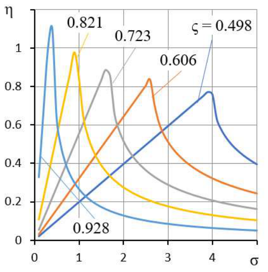
Figure 9 shows the dependence of the degree of stability η on the parameter σ for different values of ς.
These dependencies are also clearly extreme in relation to the parameter σ. This means that for each set of values of χ and ς, there is an optimal σ that provides the best thrust bearing dynamics.
To determine the optimal σ, we reduce the characteristic equation (57) to a normalized form [26]:
whereEquation (58) has two multiple roots q = –1, for which η0 =1, when a = 2. It follows that the optimal value of the “compression number” σ is determined by the formula
1 + aq + q2 = 0,
Figure 10 shows the graphs of σoptversus the coefficient ς, which clearly monotonically decreases. This means that the larger ς is, the smaller the optimal value of σopt. Conversely, the larger χ is, the larger σoptis, which provides the thrust bearing with optimal dynamic performance.
Figure 10.
Graphs of the dependence σopt (ς) for different values of the coefficient χ.
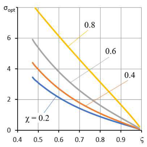
When a thrust bearing is designed, the desired values of χ and ς can be selected on the basis of the static performance requirements; then, formula (60) can be used to calculate σopt,and (21) can be used to find the design gap h0. To do this, one needs to substitute the current time scale into (21) and, after simple transformations, find the formula required for the calculations
An analysis of the dynamic criteria revealed that the parameter σ can be considered a measure of thrust bearing damping. Indeed, at low σ, the thrust bearing motion oscillates, indicating a small safety margin due to insufficient damping of the lubricant film. As shown in Figure 6, with increasing σ, the thrust bearing dynamics improve, reaching their optimal state. However, with further increases in this parameter, damping becomes unnecessary, as the transient response time significantly slows. This will negatively impact the quality of metalworking when the design is used in metal-cutting equipment. To ensure optimal thrust bearing dynamics, it is recommended that σ = σopt.
The theoretical findings were verified using an alternative finite-difference method, as well as a simplified approach that assumes a linear pressure distribution within the gap as a function of the radius. The first method yielded identical results, while the second produced minor, expected deviations—though these remain qualitatively consistent with the overall conclusions.
10. Conclusions
This paper examines the design of a stepped axial aerostatic thrust bearing with an opposed lubrication system. A mechanism for increasing the load-bearing capacity through the use of an opposed system alone is described. A mathematical model of the static and dynamic state of the structure is formulated. Methods for calculating the bearing capacity, compliance, and lubricant flow rate of thrust bearings have been developed. The calculations are performed in dimensionless form. The use of an opposed lubrication system in combination with a stepped axial gap design enables the realization of virtually maximum load-bearing capacity values, for which the utilization of the bearing surface area can reach 95% or more, whereas in a thrust bearing with an opposed system and a flat gap, this value is approximately 75%, and in a conventional thrust bearing, it is approximately 50%. The main conclusion is that using a stage in combination with an opposed system significantly increases the bearing capacity, which is 20% to 30% greater than that of a thrust bearing with an opposed system and a flat gap and almost twice that of a conventional thrust bearing. Moreover, compliance can be reduced by a factor of 2--3, and the fluid flow rate can be reduced by at least an order of magnitude. A study of the dynamic performance criteria revealed that there are optimal values for the pressure settings χ and ς, as well as the "compression number" σ, which determines the optimal damping of the lubricant film in terms of response speed and absolute stability margin.
Author Contributions
Conceptualization, VK; Methodology, V.K., A.Ku, and O.G.; Software, VK; Validation, O. G. and A. Kr.; Formal analysis, A.Kr.; Investigation, A.Kr.; Resources, A. Kr.; Data curation, A.Ku; Writing—original draft, A.Ku. and A.Kr.; Writing—review and editing, A.Ku.; Visualization, A.Ku.; Supervision, A.Kr.; Project administration, VK; Funding acquisition, A.Kr. All the authors have read and agreed to the published version of the manuscript.
Funding
This research received no external funding.
Notations
| Forces and compliance: | |
| f, F | dimensional and dimensionless load |
| f0, F0 | dimensional and dimensionless design load |
| fin, Fin | dimensional and dimensionless inertial forces of the thrust runner mass |
| w, W | dimensional and dimensionless load-carrying capacity |
| wl, W l | dimensional and dimensionless ultimate load-carrying capacity |
| K | dimensionless compliance of the thrust bearing |
| Radii and lengths: | |
| r, R | current dimensional and dimensionless radii |
| r0 | outer radius of the thrust bearing, radii scale factor |
| r1, R1 | dimensional and dimensionless mean radius |
| r2, R2 | dimensional and dimensionless inner radius |
| l1, l2, L1, L2, | dimensional and dimensionless length of radial channels |
| Gaps: | |
| h0, | dimensional design gap, gap scale factor |
| h, H | dimensional and dimensionless outer axial gaps |
| hm, Hm | dimensional and dimensionless axial gaps in the step region |
| hr, Hr | dimensional and dimensionless radial gaps |
| Pressures: | |
| ps | external pressure, pressure scale factor |
| pc, Pc | dimensional and dimensionless pressure at the inlet to the axial gap |
| pm, Pm | dimensional and dimensionless pressure at the inlet to the step |
| p, P | dimensional and dimensionless pressure functions |
| Flow rates: | |
| qh, Qh | dimensional and dimensionless flow rates in the outer axial gap |
| qm, Qm | dimensional and dimensionless flow rates in the step gap |
| qr, Qr | dimensional and dimensionless flow rates in the radial gap |
| Parameters: | |
| m | mass of the heel |
| δ, Δ | dimensional and dimensionless height of the step |
| χ, ς | design pressure tuning coefficients Pc and Pm |
| σ | "compression number" |
| µ | dynamic viscosity of the lubricant |
| t, τ | dimensional and dimensionless current time |
| Criteria of dynamic quality: | |
| η, | degree of stability of the dynamic system |
| η0, | normalized degree of stability of the dynamic system |
| ξ | oscillation decay criterion per period |
References
- Yu, X.; Gao, W.; Feng, Y.; et al. Research Progress of Hydrostatic Bearing and Hydrostatic-Hydrodynamic Hybrid Bearing in High-End Computer Numerical Control Machine Equipment. Int. J. Precis. Eng. Manuf. 2023, 24, 1053–1081. [Google Scholar] [CrossRef]
- Yu, X.; Qiao, W.; Zhang, C.; et al. Performance investigation of hydrostatic thrust bearing with double rectangular cavity under extreme working conditions. J. Braz. Soc. Mech. Sci. 2026. Eng. 48, 78. [CrossRef]
- Zhang, G.; Huang, M.; Chen, G.; Li, J.; Liu, Y.; He, J.; Zheng, Y.; Tang, S.; Cui, H. Design and optimization of fluid lubricated bearings operated with extreme operating performances—a comprehensive review. Int. J. Extrem. Manuf. 2024, Volume 6, Number 2. [Google Scholar] [CrossRef]
- Zhang, Y.; Li, J.; Wu, Y.; Wang, M.; Kong, P. Study of the lubricity of oil film at constant cutting speed under different loads of a hydrostatic turntable. Tribol. Trans. 2023, 66(1), 135–143. [Google Scholar] [CrossRef]
- Labuda, W.; Wieczorska, A. Possibility of Using the Hydrostatic Burnishing Process in Marine Conditions. Adv. Sci. Technol. Res. J. 2024, 18(6). [Google Scholar] [CrossRef] [PubMed]
- 6. Zhang, G.; Huang, M.; Chen, G.; Li, J.; Liu, Y.; He, J.;... Cui, H. Design and optimization of fluid lubricated bearings operated with extreme operating performance—a comprehensive review. Int. J. Extrem. Manuf. 2024, 6(2), 022010. [CrossRef]
- Hanawa, N.; Kuniyoshi, N.; Miyatake, M.; Yoshimoto, S. Static characteristics of a water-lubricated hydrostatic thrust bearing with a porous land region and a capillary restrictor. Precis. Eng. 2017, Volume 50, 293–307. [Google Scholar] [CrossRef]
- Nishitani, Y.; Yoshimoto, S.; Somaya, K. Numerical investigation of static and dynamic characteristics of water hydrostatic porous thrust bearings. Int. J. Autom. Technol. 2011, T. 5.(No. 6), 773–779.5. [Google Scholar] [CrossRef]
- Kodnyanko, V.; Kurzakov, A. Static characteristics and dynamic quality of a hydrostatic thrust bearing with the opposite lubrication system. Precis. Eng. Vol. 2026, Volume 101, 395–402. [Google Scholar] [CrossRef]
- Kodnyanko, V.; Kurzakov, A. Performance of annular hydrostatic opposed-pad thrust bearing with opposite lubrication system. 2026. Available online: https://ssrn.com/abstract=6598832. [CrossRef]
- Marinescu, A.; Cicone, T.; Fatu, A. The study of a novel hydrostatic thrust bearing with a structurally elastic component: Theory and experiments. Tribol. Int. 2023, 189, 108954. [Google Scholar] [CrossRef]
- Huang, H. C.; Yang, S.H. Thrust-bearing layout design of a large-sized hydrostatic rotary table to withstand eccentric loads for horizontal boring machine applications. Lubricants 2022, 10(4), 49. [Google Scholar] [CrossRef]
- Kodnyanko, V.; Kurzakov, A.; Surovtsev, A.; Strok, L.; Grigorieva, O.; Brungardt, M.; Belyakova, S.; Gogol, L. Theoretical Study of the Static and Dynamic Characteristics of a Slotted Adaptive Hydrostatic Thrust Bearing with a Regulator of the Lubricant Output Flow. Mathematics 2022, 10(3), 355. [Google Scholar] [CrossRef]
- Kodnyanko, V. Method for Calculating the Static Characteristics of Radial Hydrostatic Compensator of Machine Tool Bearings Deformation. Period. Polytech. Transp. Eng. 2021, 49(2), 114–119. [Google Scholar] [CrossRef]
- Kodnyanko, V.; Kurzakov, A.; Grigorieva, O.; Brungardt, M.; Belyakova, S.; Gogol, L.; Surovtsev, A.; Strok, L. Theoretical Disquisition on the Static and Dynamic Characteristics of an Adaptive Stepped Hydrostatic Thrust Bearing with a Displacement Compensator. Mathematics 2021, 9, 2949. Available online: https://www.mdpi.com/2227-7390/9/22/2949. [CrossRef]
- Kodnyanko, V.; Belyakova, S.; Grigorieva, O.; Gogol, L.; Surovtsev, A.; Strok, L. The use of a displacement compensator to improve the static characteristics of a step hydrostatic thrust bearing. J. Res. Mech. Eng. 2021, Volume 7(Issue 7), pp: 11–16. [Google Scholar]
- Pinegin, S.V.; Tabachnikov, Yu.V.; Sinenkov, I.E. Static and Dynamic Characteristics of Gas-Static Bearings; (in Russian). Nauka: Moscow, 1982. [Google Scholar]
- Kodnyanko, V. Optimal Section Method for Minimizing Unimodal Functions. Comput Math. Model 2025. [Google Scholar] [CrossRef]
- Wardle, F. 3 – Hydrostatic bearings ISBN 9780857091628; Woodhead Publishing, 2015; pp. 147–225. [Google Scholar] [CrossRef]
- Kodnyanko, V. Dynamic modeling of negative compliance hydrostatic thrust bearing with Laub's elastic orifice. Meccanica 2026, 43. [Google Scholar] [CrossRef]
- Rehman, W.U.; Ullah, N.; Anjum, Z.; Aslam, M.A.; Lodhi, E.; Razzaq, M.A. A mechatronics approach for active control of hydrostatic thrust bearing using fopid control techniques. Spectr. Eng. Sci. 2025., 576–585. [Google Scholar] [CrossRef]
- Bently, D.E.; Grant, J. W.; Hanifan, P.C. Active controlled hydrostatic bearings for a new generation of machines. In Turbo Expo: Power for Land, Sea, and Air;2000. p. V002T03A011; American Society of Mechanical Engineers; Vol. 78552. [CrossRef]
- Rehman, W.U.; Jiang, G.; Luo, Y.; Wang, Y.; Khan, W.; Rehman, S.U.; Iqbal, N. Control of active lubrication for hydrostatic journal bearing by monitoring bearing gap. Adv. Mech. Eng. 2018, 10(4), 1687814018768142. [Google Scholar] [CrossRef]
- Teo, C. J.; Spakovszky, Z.S. Modeling and experimental investigation of microhydrostatic gas thrust bearings for micro- turbomachines. 2006. [Google Scholar] [CrossRef]
- Li, X.; Wang, X.; Li, M.; Ma, Y.; Huang, Y. The research status and progress of heavy/large hydrostatic thrust bearing. Adv. Mech. Eng. 2014, 6, 982584. [Google Scholar] [CrossRef]
- Doetsch, G. Introduction to the Theory and Application of the Laplace Transformation; Springer Science & Business Media, 2012. [Google Scholar]
- Besekersky, V.A.; Popov, E.P. Theory of automatic control systems; Profession: Moscow, 2003. [Google Scholar]
- Popov, E.P. The dynamics of automatic control systems; Elsevier, 2014. [Google Scholar]
Figure 1.
Diagram of the annular hydrostatic gap.
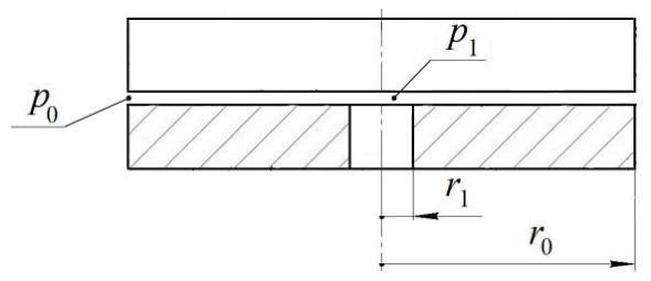
Figure 2.
Steped hydrostatic thrust bearing with the opposite lubrication system.
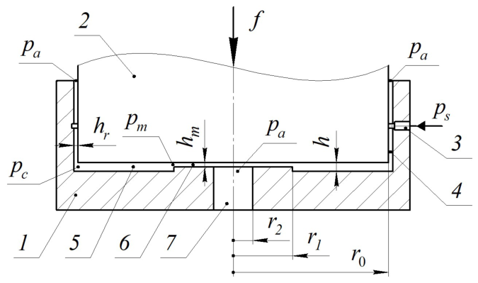
Figure 3.
Graphs of the dependence Hm (F) for different values of the coefficient ς.
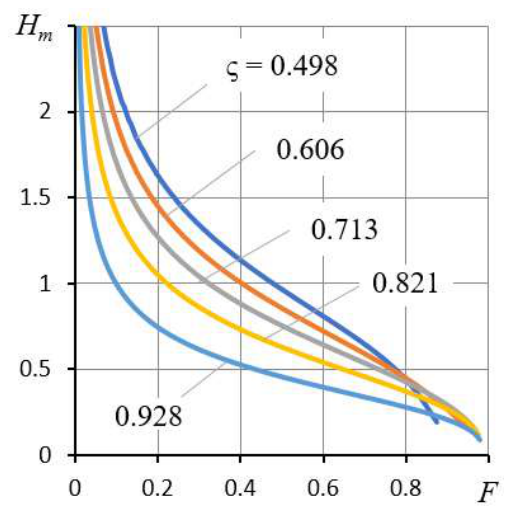
Figure 4.
Graphs of the dependence K (F) for different values of the coefficient ς.
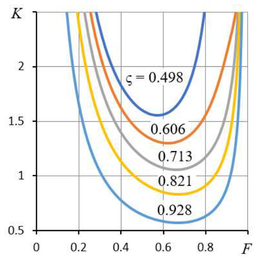
Figure 5.
Graphs of the dependences Qs (F) for different values of the coefficient ς.
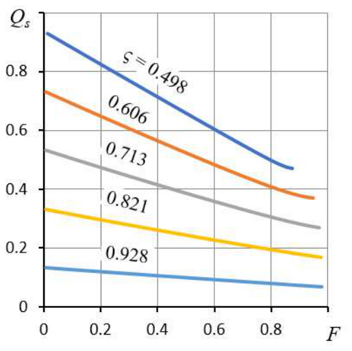
Figure 6.
Graphs of the dependence η (ς) for different values of the coefficient χ for σ = 0.8.
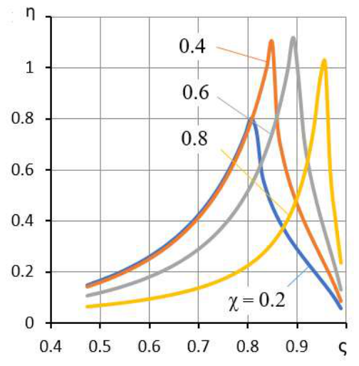
Figure 7.
Graphs of the dependence ξ (ς) for different values of the coefficient χ for σ = 0.8.
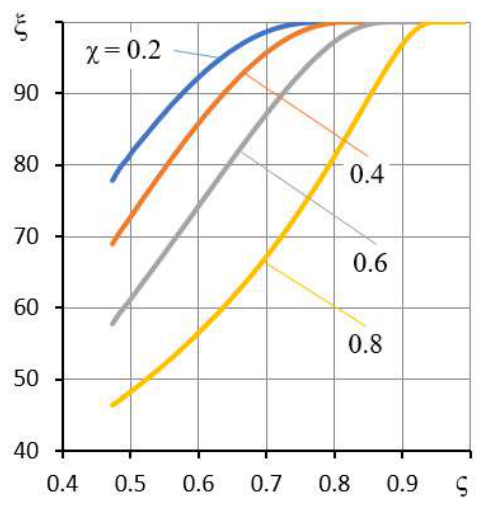
Figure 8.
Graphs of the dependence η0 (ς) for different values of the coefficient χ for σ = 0.8.
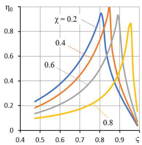
Figure 9.
Graphs of the dependence η (σ) for different values of the coefficient ς for χ = 0.4.
Disclaimer/Publisher’s Note: The statements, opinions and data contained in all publications are solely those of the individual author(s) and contributor(s) and not of MDPI and/or the editor(s). MDPI and/or the editor(s) disclaim responsibility for any injury to people or property resulting from any ideas, methods, instructions or products referred to in the content. |
© 2026 by the authors. Licensee MDPI, Basel, Switzerland. This article is an open access article distributed under the terms and conditions of the Creative Commons Attribution (CC BY) license (http://creativecommons.org/licenses/by/4.0/).
Copyright: This open access article is published under a Creative Commons CC BY 4.0 license, which permit the free download, distribution, and reuse, provided that the author and preprint are cited in any reuse.