

Submitted:
11 November 2026
Posted:
13 November 2026
You are already at the latest version
Abstract
To define a new physical quantity, convergence, characterizing celestial bodies, the energy-momentum field is examined. The energy-momentum field tensor is calculated, describing the gradients in distribution of the four-potential within the physical system under consideration. The energy-momentum field equations are solved, and the scalar potential of the field is determined as a function of radial coordinate. Since the four-potential of the energy-momentum field is a primary component of the four-momentum density, this allows for derivation of the system's energy density as a function of radial coordinate. Energy convergence is defined as the ratio of the average energy density of a celestial object to the corresponding value for a typical neutron star. Similarly, mass convergence is defined as the ratio of the average mass density of a celestial object to the average mass density of a neutron star. The discrepancy between the formulas for energy convergence and mass convergence results in a slight difference between the two convergence values, stemming from the difference between the formulas for inertial and gravitational mass.
Keywords:
energy-momentum field
; four-momentum density
; energy convergence
; mass convergence
1. Introduction
There are known studies in which the functions and parameters describing the state of massive celestial bodies are derived based on a relatively simple theoretical model. For instance, the polytropic model assumes that the gas pressure within a star is related to mass density by a polytropic equation [1]. In [2], a planet or star is treated as a relativistic uniform system subject to gravitational, electromagnetic, acceleration, and pressure fields, among others. In [3], the equations of hydrostatic equilibrium for compact stars are solved by parameterizing the dependence of matter density on the radius.
More precise theoretical models employ techniques for the simultaneous solution of multiple equations of state for matter and incorporate additional conditions and theoretical constraints, such as the continuity equation, equations for specific phase states of matter, metric equations, equations of motion for matter particles, field equations, thermodynamic equations, and so forth. Furthermore, quantum and relativistic effects within the matter of compact objects are taken into account [4].
One of the authors of this work, H.B., has suggested that the description of massive material bodies, and even elementary particles, as used in modern physics is incomplete and could be refined. To understand this, one must examine global models of physical reality that encompass a wide variety of cosmic objects. An analysis of such models reveals that they incorporate the following fundamental principles for organization of cosmic structures:
a) The principle of hierarchy – cosmic structures belong to specific levels of matter, depending on their size [5,6,7]. At the primary levels of matter, the objects that make up cosmic structures reach their maximum mass and energy density. Typical examples include the nucleon at the nucleonic level of matter and the neutron star at the stellar level. Intermediate levels of matter exist between these primary levels [8,9].
b) The principle of discreteness – levels of matter are discrete; each level is characterized by its own specific range of masses and sizes for the cosmic structures it contains [10,11].
c) The principle of similarity between levels of matter – the masses and dimensions of cosmic structures at adjacent levels of matter correspond to one another and increase according to a geometric progression [9,12,13].
d) The principle of nestedness – every structure at a given level of matter contains within itself, and is composed of, structures from lower levels of matter. For instance, the metagalaxy consists of galaxies, galaxies consist of stars, stars consist of atoms and nucleons, and so on [14].
e) The principle of fractality – cosmic structures at different levels of matter exhibit corresponding morphology, kinematics, and dynamics [15,16].
f) The principle of structural evolution – a multitude of structures at lower levels of matter, under the influence of physical forces, coalesce into a single whole; in the course of evolution, this entity decreases in size and transforms into a single, massive structure of a higher level of matter. A typical example is the evolution of stellar matter during continuous gravitational collapse [17,18], in which a multitude of atoms within a gas cloud coalesce to form a stellar object.
These principles describe the theory of infinite hierarchical nesting of matter. They also apply to the entire diversity of living organisms [19,20,21,22,23,24]. The principles presented suggest that the physical forces acting at different levels of matter are similar in their mode of operation. To describe the invariance of physical laws, the SPF-symmetry is introduced in [9], a concept wherein the equations of motion remain unchanged when the scales of size, mass, and velocity of physical processes are simultaneously altered. The principle of hierarchy leads to the notion of scale dimension [25,26,27,28] as the fifth spatial dimension. All cosmic structures can be positioned along the scale dimension axis according to their respective sizes.
The principle of relativity, well-known in classical physics, which underpins the invariance of physical laws in inertial reference frames and forms the basis for the special theory of relativity, can be combined with scale dimension to yield a scale-dependent special theory of relativity; in this framework, the equations of physics should remain invariant in form when transitioning from one level of matter to another [29].
In contrast, scale relativity, as developed in the work of Laurent Nottale, emerges from a synthesis of the principle of relativity, the principle of fractality, and quantum mechanics, allowing physical properties of particles, such as mass and charge, to be derived from the geometric properties of spacetime. To this end, the reference frame incorporates an additional scale coordinate with fractal properties, rendering the frame dependent on the scale. Scale transformations give rise to effects such as time dilation and length contraction, which vary according to the scale [30], with the Planck length serving as an invariant limiting scale. In [31], the quantization of planetary orbits in the Solar System is described based on scale relativity and the principles of quantum mechanics. Accounting for scale transformations makes it possible to apply quantum mechanics and gauge field theories to astrophysics, cosmology, and complex systems [32].
Thus, research within the theory of infinite hierarchical nesting of matter, the theory of fractal Universe, and the scale-relativity approach to field theory demonstrates that cosmic structures and the objects that compose them are similar to one another in terms of their kinematics and dynamics, that is, in terms of their physical parameters and the equations of state for matter. Consequently, in order to account for the changes in the size of cosmic objects over time, it becomes necessary to introduce "convergence" as a new physical quantity.
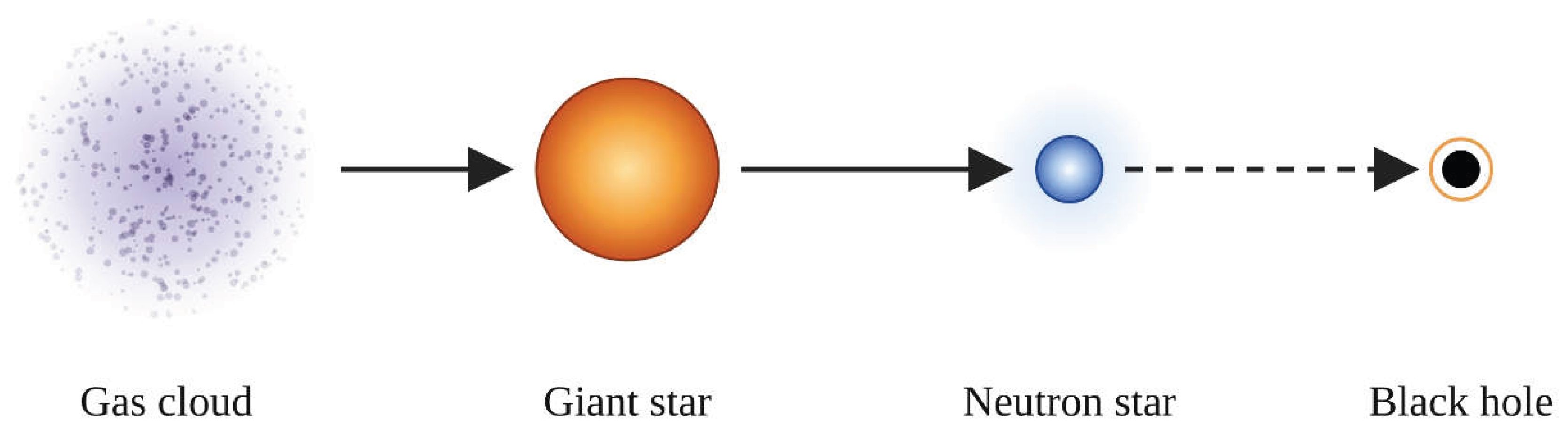
On one hand, convergence of mass can be viewed as a process in the evolution of a cosmic object, during which its mass density continuously increases. Figure 1 illustrates this process, showing a massive star forming from a gas cloud through gravitational collapse. The subsequent evolution of the star may lead to the creation of a neutron star, with a potential further transformation into a black hole.
According to the theory of stellar evolution [33], a hydrogen gas cloud with a size on the order of – m and a mass ranging from 3 to 9 solar masses initially contracts into a protostar of the same mass, with a radius between and 100 solar radii, surrounded by a dense dust envelope. During the nuclear-burning stage, a star with the mass of 9 solar masses has the radius of approximately 4.4 solar radii. Once its nuclear fuel is exhausted, such the star may, following a supernova phase, give rise to a neutron star with a typical mass of 1.35 solar masses and radius of 12 km. Thus, convergence of mass implies that matter is compressed by gravitational forces into a small volume with high mass density.
On the other hand, the mass convergence within a given object can be understood as a physical quantity describing the degree of mass concentration in that object. The same applies to the energy convergence within such the object. If convergence is considered a scalar quantity, then the rate of convergence becomes a vector quantity, depending on the direction in which the convergence changes most rapidly. As observations show, the accumulation of mass in cosmic objects typically occurs in a radial direction toward the center of mass of these objects.
In this context, one of the aims of this work is to determine the mass and energy convergences within a sufficiently large physical system held together against disintegration by gravitational forces. The quantities of mass and energy per unit volume of a system are defined by the well-known parameters of mass density and energy density. General relativity employs a quantity that characterizes the compactness of a physical system, defined by the ratio , where is the gravitational radius, is the gravitational constant, and are the system's radius and mass, respectively [34]. The greater the mass contained within the sphere of radius , the higher the value of compactness .
In contrast, the terms of mass and energy convergences are used in this article to refer to relative values that can be employed to assess the degree of concentration of mass and energy within objects at any level of matter. For the sake of clarity, we shall focus our discussion on planets and stars, which belong to the stellar form of matter.
The structure of the article is as follows. In Section 3.1, we examine gradients in the four-momentum density distribution within a physical system. To this end, we calculate the energy-momentum field tensor, derived from the curl of the energy-momentum field's four-potential density. Solving the energy-momentum field equation in Section 3.2 yields formulas for the scalar and vector potentials of the field. Subsequent analysis in Section 3.3 makes it possible to estimate the value of the energy-momentum field constant , which appears in the Lagrangian density and the field equation, and to determine the energy convergence. Section 3.4 defines the mass convergence of a cosmic object.
2. Method
In [35], the energy-momentum vector field was introduced, characterized by the four-potential , the field tensor , and the stress-energy tensor . The principle of least action allows for derivation of equation for the metric, the equation of motion for matter particles, and the equations satisfied by the components of four-potential. The components of the four-potential can be expressed as , where is the scalar potential with the dimensions of volumetric energy density, is the vector potential of the energy-momentum field with the dimensions of momentum density, and is the speed of light.
By simultaneously solving the equation for the metric, the equation of motion, and the equations for the energy-momentum field, one determines the components of the metric tensor, the components of the four-velocity, and the components of the four-potential .
The four-momentum density of a physical system is defined via derivative of the Lagrangian density with respect to the four-velocity :
The Lagrangian density accounting for the energy-momentum field has the following form:
In (2), is the scalar curvature; is the cosmological constant; and are certain constants to be determined. Here, the constant appears in the equation for the metric, while the constant appears in the equation for the energy-momentum field.
Substituting (2) into (1) yields an expression for the system's four-momentum density, which includes the four-potential of the energy-momentum field:
Taking (1-3) into account, the four-momentum of the system is expressed as integral over the three-dimensional volume:
In (4), is the time component of the four-velocity , and is the determinant of the metric tensor with metric signature .
3. Results
3.1. Four-Momentum Density
Analogously to [36], we express the four-momentum density (1) in terms of components in four-dimensional Cartesian coordinates as follows:
The quantity in (5) represents the energy density, while the quantity represents the density of the three-dimensional momentum vector of an arbitrary element of matter or a typical particle characterizing the continuously distributed matter of a given body.
Using the four-curl operator acting on (5), we define the tensor associated with the four-momentum density:
We express the non-zero components of the tensor (6) in terms of the components (5):
Let us introduce a three-dimensional vector and a three-dimensional solenoidal vector in the following form:
As a result, the components of the tensor can be expressed in terms of the components of the vectors and :
Note that in Cartesian coordinates, the components of four-dimensional vectors are the physical components through which the interaction of particles and fields takes place. In curvilinear coordinates, the components of four-dimensional vectors differ from the corresponding physical components due to the appearance of Lamé coefficients. Consequently, the forms of differential operators acting on physical components in curvilinear coordinates do not coincide with those of the corresponding operators in Cartesian coordinates.
In what follows, we shall use spherical four-dimensional coordinates , which are convenient for studying the properties of spherically symmetric objects such as planets and stars. Let the three-dimensional momentum density vector in spherical coordinates have physical components . Then, formulas (8) for the vectors and transform as follows:
The vector (10) is calculated using partial derivatives with respect to time and spherical coordinates , taken from the components and of the four-momentum density (5). The formulas presented above correspond in form to those for the electromagnetic field; thus, the vector is analogous to the electric field strength , while the vector corresponds to the magnetic field induction . Consequently, the vector reflects the linear aspects of gradients of the four-momentum density components, whereas the vector is associated with the rotational aspects of gradients of the four-momentum density components.
Let us consider the limiting case where the components of the momentum density vector of matter elements of a certain spherical body are small in magnitude. If the energy density distribution within the body is spherically symmetric and the body is in a state of equilibrium – neither rotating nor moving within an inertial reference frame – then, after time averaging, the partial time derivatives in (10) can be assumed to be zero. Assuming that the energy density does not depend on the angles , we find from (10):
Typically, the energy density in celestial bodies is maximal at the center and decreases as the radial coordinate increases. This results in the quantity in (12) being positive.
3.2. Solution of Equation for Four-Potential of Energy-Momentum Field
According to [35], the equation for determining the four-potential of energy-momentum field has the following form:
Equation (13) can be written as follows:
For an arbitrary four-vector , the rule for difference of double covariant derivatives is known:
In (15), we replace with , express the quantity , and substitute it into (14):
In (16), we apply the gauge condition for the four-potential in the form . To simplify, we consider equation (16) within the framework of special theory of relativity, where the Riemann curvature tensor vanishes and the operator reduces to the d'Alembert operator . Taking this into account, equation (16) yields the equation
Since the four-potential of the energy-momentum field has components of the form , in special theory of relativity it will be . Taking into account also that in the case under consideration
where is the Lorentz factor, equations for the scalar potential and the vector potential follow from (17-18):
Let us choose a point within the body and a small region of space surrounding that point. After averaging over the volume of this region and over time, taking into account the random motion of typical particles of matter, it can be assumed that, in a stationary body, the magnitudes of the potentials and do not depend on time. Since the particle velocity is zero after volume averaging, the vector potential in (20) will also be zero on average. Taking this into account, it follows from (19) that:
Equation (21) represents the averaged scalar potential of the energy-momentum field. For a spherical body, it is convenient to use spherical coordinates , in terms of which the Laplacian (21) should be expressed. This yields the equation
In (12), it was assumed that the energy density within the spherically symmetric body does not depend on the angles . Assuming the same for the scalar potential , we simplify equation (22):
For the case where the spherical body under consideration is a relativistic uniform system, the dependence of Lorentz factor on the radial coordinate was found in [37]:
In (24), is the Lorentz factor of particle motion at the center of the spherical body, is the acceleration field coefficient, and is the invariant particle mass density. Substituting (24) into (23) leads to the equation
and to the solution of equation (25):
3.3. Energy Convergence
In [35], the tensor of energy-momentum field is calculated using the formula
where the four-potential is .
In the approximation under consideration, the vector potential vanishes on average according to (20), while the scalar potential (26) depends on the radial coordinate . Consequently, the tensor (27) depends on the radial coordinate but is independent of the four-velocity . If we further assume that and the scalar curvature makes no contribution to the four-momentum density, it follows from (3) that . Taking this and the definition (5) into account, we find that the scalar potential (26) can be replaced by the energy density appearing in the time component of the four-momentum density . This yields the following:
If we let the radial coordinate approach zero in (28), the energy density will approach the value at the center of the body; here , since we must have to avoid an infinitely large energy density value. Taking this into account, we obtain
Expressing from (29) and substituting it into (28), we find:
Let us average the energy density (30) over the volume of a sphere of radius , bearing in mind that in spherical coordinates the volume element is :
(31)
We substitute the energy density (30) into (12) and evaluate the quantity as a function of the radial coordinate:
Averaging (32) over volume of the spherical body yields the following:
We use the first relation for the four-momentum (4) and derive from it an expression for the time component :
According to the definition of the four-momentum, the time component of the four-momentum is , where and denote the energy and momentum of the physical system. In (5), the time component of the four-momentum density is . In special theory of relativity, the four-velocity takes the form (18), so the time component of the four-velocity is . Taking this into account, (34) can be written as:
In spherical coordinates, the metric tensor in special theory of relativity has the following form:
From (36), we find the determinant of the metric tensor and the quantity :
Substituting the quantities (24), (30), and (37) into (35), and taking into account the relation , we obtain:
According to [38], in relativistic uniform model for uncharged matter, the acceleration field constant is expressed in terms of the gravitational constant by the formula
Next, we consider the case where absolute value of gravitational potential at the surface of the massive body in question is sufficiently small compared to the square of the speed of light, such that . The gravitational mass of the body can be estimated using the formula . Taking this into account and using (39), one can compare the third and fourth terms within the parentheses on the right-hand side of (38):
Taking (40) into account, the fourth term in the parentheses on the right-hand side of (38) can be neglected. Let us also express the energy of the stationary body using Einstein's formula as , where denotes the inertial mass of the body, accounting for all acting fields. This leads to the relation
The second term in the parentheses on the right-hand side of (41) is associated with the contribution from the chaotic motion of particles within the body; in terms of order of magnitude, it represents the ratio of the square of the particle velocity to the square of the speed of light . Similarly, the third term in the parentheses on the right-hand side of (41) is, in terms of order of magnitude, the ratio of the square of the particle velocity induced by fields to the square of the speed of light . In massive bodies, the gravitational field is to be considered the primary field; its effect is maximal near the body's surface, where . In this context, the square of the particle velocity induced by the field is determined by the gravitational potential at the body's surface. Taking this into account, one can formulate a relation for the third term in the parentheses on the right-hand side of (41) that allows for estimation of the energy-momentum field coefficient up to a small numerical factor:
In the approximation under consideration, the energy density at the center of the body can be taken as , and the gravitational mass depends on the mass density , the body's volume , and the Lorentz factor at the center of the body [39]. Taking this into account, we find the following first-order approximation for the energy-momentum field constant in (42):
The constant (43) includes the mass density, which is considered constant in the energy-momentum field concept [35].
Substituting (43) into (31), taking into account the relations , , , yields an estimate for the average energy density of the massive body:
Now let us substitute (43) into (33), taking into account the relations , , , and estimate the value of :
According to (45), the rate of change of energy density along the radial coordinate, averaged over the volume of the massive body, is proportional to the body's radius and the square of the energy density at its center.
Let us define energy convergence in cosmic stellar objects as a relative quantity, expressed as the ratio of the stellar object's average energy density to the average energy density of a neutron star. Taking (44) into account, we have:
Taking into account (44) and the relation , the average energy density of a neutron star is determined by the formula:
A typical neutron star has the mass , where is the mass of the Sun, and the radius km, yielding the mass density on the order of kg/m³. According to [40], the Lorentz factor for the motion of typical particles at the center of the neutron star reaches the value of . Substituting these values into (47), we find the average energy density of the neutron star to be J/m³. Thus, if the average density of a cosmic object reaches the value , the convergence (46) becomes equal to 1.
3.4. Mass Convergence
In addition to energy convergence (46), one can define mass convergence as the ratio of the average mass density of a stellar object to the average mass density of a neutron star:
According to [41], the mass density inside a stationary spherical body representing a relativistic uniform system is . Substituting the Lorentz factor (24) into this expression and averaging over the body's volume , we find the average density :
From (48-49), the expression for mass convergence follows:
4. Discussion of Results
As seen in (46) and (50), the expressions for energy convergence and mass convergence do not coincide. This is because the system's inertial mass (41) is derived from the energy , whereas in relativistic uniform system with active vector fields, the invariant mass of all the system's particles equals the system's gravitational mass [40,42]. The difference between the formulas for determining inertial and gravitational masses leads to a difference between the convergences and . However, the difference between inertial and gravitational masses is small and is significant only for compact stars such as white dwarfs and neutron stars. The same applies to the convergences and .
The formulas presented above are applicable not only to celestial bodies such as planets and stars but also to particles at the atomic level of matter, where the primary entities are electrons, the nucleons constituting atomic nuclei, and other similar particles. For instance, a proton model is discussed in [43,44] in which strong gravitation between nucleons and within the matter of the nucleons themselves, plays the same role as ordinary gravitation between stars and within stellar matter. Similarly, a photon model is presented in [45], in which the particles constituting the photon are held together by strong gravitation and electromagnetic forces. Thus, replacing the gravitational constant with the strong gravitational constant allows the derived results to be applied to particles at the atomic level. In particular, is used to calculate the fine-structure constant, the proton's rest energy, and its radius [9,14], while the structure of the photon is determined in [45], as well as its dimensions and rest mass.
From the perspective of the theory of infinite hierarchical nesting of matter and Le Sage's theory of gravitation, the existence of gravitational constants and reflects the differing properties of gravitons acting at various levels of matter [46,47,48]. Taking this circumstance into account, and based on the structure of electrogravitational vacuum populated by various types of gravitons, the article [49] presents the operating principle of a spacecraft engine that draws energy from the electrogravitational vacuum. Thus, if one takes into account how the properties of gravitons and charged vacuum particles vary depending on the chosen level of matter, the definitions of mass and energy convergences can be applied to any objects existing in nature.
5. Conclusions
To study energy convergence in celestial bodies, in (6) we introduce the tensor related to the four-momentum density of typical particles or matter elements within these bodies. In (9), the components of the tensor are expressed in Cartesian coordinates in terms of the components of vectors and . Equations for determining the vectors and in spherical coordinates are presented in (10-11).
In Section 3.2, equation (13) for the four-potential of the energy-momentum field is solved, and a solution for the scalar potential is obtained in (26) within the framework of the relativistic uniform model.
For stationary bodies in equilibrium state, the components of the vector and the components of the vector potential can be neglected. Assuming also that the scalar curvature and the tensor make a negligible contribution to the four-momentum density (3), we arrive at the relations , . The energy density , averaged over the body's volume, leads to the value (44), which makes it possible to determine, in (46), the energy convergence in cosmic bodies.
In (38), it is shown that the system's energy depends on the constant of the energy-momentum field. Assuming that gravitational field is the primary active field in the system, an estimate of the constant is made in (43). A more precise value of can be obtained by taking into account other vector fields, such as the acceleration field, the pressure field, and the electromagnetic field. Using the constant , the average energy density (44) and the average value (45) of the radial component of the vector (12) are estimated.
Unlike energy convergence , mass convergence (50) is calculated using a different method that accounts for dependence of mass density on the Lorentz factor of moving particles of matter. Energy convergence and mass convergence are relative quantities indicating the difference between the average energy density and average mass density of a cosmic body and corresponding values for a typical neutron star.
Availability of data and materials
Not applicable.
Competing interest
The authors have no relevant financial or non-financial interests to disclose.
Authors' contributions
Not applicable.
Clinical trial number
Not applicable.’
Ethical approval
Not applicable.
Consent to participate
Not applicable.
Consent to publish
Not applicable.
Funding
No funds, grants, or other support was received.
Acknowledgements
Not applicable.
References
- Herrera, L.; Barreto, W. Newtonian polytropes for anisotropic matter: General framework and applications. Phys. Rev. D. 2013, 87, 087303. [Google Scholar] [CrossRef]
- Fedosin, S.G. Estimation of the physical parameters of planets and stars in the gravitational equilibrium model. Can. J. Phys. 2016, Vol. 94(No. 4), 370–379. [Google Scholar] [CrossRef]
- Rodrigues, H. Modeling compact stars without numerical integration. Eur. J. Phys. 2013, Vol. 34, 667. [Google Scholar] [CrossRef]
- Bisnovatyi-Kogan, G.S.; Patraman, E.A. Uniform models of neutron and quark (strange) stars in general relativity; Astrophysics, 2026. [Google Scholar] [CrossRef]
- Somerville, R.S. Galaxy formation in the hierarchical universe. In Joint Evolution of Black Holes and Galaxies; CRC Press, 2006; pp. 139–205. [Google Scholar] [CrossRef]
- Springel, V.; White, S.; Jenkins, A.; et al. Simulations of the formation, evolution and clustering of galaxies and quasars. Nature 2005, Vol. 435, 629–636. [Google Scholar] [CrossRef] [PubMed]
- Wilding, Georg; Nevenzeel, Keimpe; van de Weygaert, Rien; Vegter, Gert; Pranav, Pratyush; Jones, Bernard J T; Efstathiou, Konstantinos; Feldbrugge, Job. Persistent homology of the cosmic web – I. Hierarchical topology in ΛCDM cosmologies. Mon. Not. R. Astron. Soc. 2021, Vol. 507(Issue 2), 2968–2990. [Google Scholar] [CrossRef]
- Oldershaw, R.L. Hierarchical Cosmology. Astrophys. Space Sci. 1992, Vol. 189(1), 163–168. [Google Scholar] [CrossRef]
- Fedosin, S.G. Fizika i filosofiia podobiia: ot preonov do metagalaktik, (Physics and Phylosophy of Similarity From Preons to Metagalaxies) Perm; 544 pp. In Russian; 1999; ISBN 5-8131-0012-1. [Google Scholar]
- Leubner, M.P. On the Origin of Discrete Cosmic Structure Scales. The Ninth Marcel Grossmann Meeting. [CrossRef]
- Gabrielli, Andrea; Sylos Labini, Francesco; Joyce, Michael; Pietronero, Luciano. Statistical Physics for Cosmic Structures; Springer Berlin: Heidelberg, 2004; ISBN 978-3-540-40745-4. [Google Scholar] [CrossRef]
- Oldershaw, R.L. Self-similar cosmological model: introduction and empirical tests. Int. J. Theor. Phys. 1989, Vol. 28, 669–694. [Google Scholar] [CrossRef]
- Sereno, Mauro. Self-similarity of the mass distribution in rich galaxy clusters up to z∼1 tracked with weak lensing. Astron. Astrophys. 2025, Vol. 696, A227. [Google Scholar] [CrossRef]
- Fedosin, S.G. The physical theories and infinite hierarchical nesting of matter; LAP LAMBERT Academic Publishing, 2014; Volume 1, p. 580. ISBN -13: 978-3-659-57301-9. [Google Scholar]
- Gaite, J. The Fractal Geometry of the Cosmic Web and Its Formation. Adv. Astron. 2019, Vol. 2019, 6587138. [Google Scholar] [CrossRef]
- Coleman, P.H.; Pietronero, L. The fractal structure of the universe. Phys. Rep. 1992, Vol. 213(Issue 6), 311–389. [Google Scholar] [CrossRef]
- Oppenheimer, J.R.; Snyder, H. On continued gravitational contraction. Phys. Rev. 1939, Vol. 56, 455–459. [Google Scholar] [CrossRef]
- Said, Khaled; Colless, Matthew; Magoulas, Christina; Lucey, John R; Hudson, Michael J. Joint analysis of 6dFGS and SDSS peculiar velocities for the growth rate of cosmic structure and tests of gravity. Mon. Not. R. Astron. Soc. 2020, Vol. 497(Issue 1), 1275–1293. [Google Scholar] [CrossRef]
- Nottale, L.; Auffray, C. Scale relativity theory and integrative systems biology: 2. Macroscopic quantum-type mechanics. Prog. Biophys. Mol. Biol. 2008, Vol. 97, 115–157. [Google Scholar] [CrossRef] [PubMed]
- Fedosin, S.G. Nositeli zhizni: proiskhozhdenie i ėvoliutsiia. (The Carriers of Life: Origin and Evolution). In Russian; Bulanin, S.-Peterburg, 2007; ISBN 978-5-86007-556. [Google Scholar]
- KirstaYu, B. Information-hierarchical organization of biosphere and problems of its sustainable development. Ecol. Model. 2001, Vol. 145(Issue 1), 49–59. [Google Scholar] [CrossRef]
- West, Geoffrey B.; Brown, James H.; Enquist, Brian J. A General Model for the Origin of Allometric Scaling Laws in Biology. Science 1997, Vol 276(Issue 5309), 122–126. [Google Scholar] [CrossRef] [PubMed]
- Goentoro, Lea. Cross-hierarchy systems principles. Curr. Opin. Syst. Biol. 2017, Vol 1, 80–83. [Google Scholar] [CrossRef] [PubMed]
- Günther, F.; Folke, C. Characteristic of Nested Living Systems. J. Biol. Syst. 1993, Vol. 1(3), 257–274. [Google Scholar] [CrossRef]
- Fournier D’Albe, E.E. Two New Worlds: I The Infra World; II The Supra World, 1907; Longmans Green: London.
- Fedosin, S.G. Scale Dimension as the Fifth Dimension of Spacetime. Turk. J. Phys. 2012, Vol. 36(No 3), 461–464. [Google Scholar] [CrossRef]
- Jung, Yun Pyo. Infinite Universe in a Mote; Sagyejul Publishing Co., 1994; p. 290 pages. [Google Scholar]
- Sukhonos, S. The structure of stable levels of organization of material world. In S.-Peterburg, Gidrometeoizdat; 1992. [Google Scholar]
- Oldershaw, R.L. Discrete Scale Relativity. Astrophys. Space Sci. 2007, Vol. 311(No. 4), 431–433. [Google Scholar] [CrossRef]
- Nottale, L. The theory of scale relativity. Int. J. Mod. Phys. A 1992, Vol. 7(20), 4899–4936. [Google Scholar] [CrossRef]
- Nottale, L.; Schumacher, G.; Gay, J. Scale relativity and quantization of the solar system. In Astronomy and Astrophysics; 1997; Vol. 322, pp. 1018–1025. [Google Scholar]
- Nottale, L. Scale relativity and fractal space-time: theory and applications. Found. Sci. 2010, Vol. 15, 101–152. [Google Scholar] [CrossRef]
- Bisnovatyi-Kogan, G.S. Stellar Physics. 2: Stellar Evolution and Stability; Springer Berlin: Heidelberg, 2011; ISBN 978-3-642-14733-3. [Google Scholar] [CrossRef]
- Nashed, G.G.L. Constraining linear form of f(R,G,T) gravity from astrophysical observations of the Pulsar U1724. Nucl. Phys. Sect. B 2025, Vol. 1018, 117065. [Google Scholar]
- Fedosin, S.G. Definition of four-momentum through energy-momentum field. Preprints 2026, 2026091977. [Google Scholar] [CrossRef]
- Fedosin, S.G. What should we understand by the four-momentum of physical system? Physica Scr. 2024, Vol. 99(No. 5), 055034. [Google Scholar] [CrossRef]
- Fedosin, S.G. The Integral Energy-Momentum 4-Vector and Analysis of 4/3 Problem Based on the Pressure Field and Acceleration Field. Am. J. Mod. Phys. 2014, Vol. 3(No. 4), 152–167. [Google Scholar] [CrossRef]
- Fedosin, S.G. The binding energy and the total energy of a macroscopic body in the relativistic uniform model. Middle East J. Sci. 2019, Vol. 5(Issue 1), 46–62. [Google Scholar] [CrossRef]
- Fedosin, S.G. Relativistic Energy and Mass in the Weak Field Limit. Jordan J. Phys. 2015, Vol. 8(No. 1), 1–16. [Google Scholar] [CrossRef]
- Fedosin, S.G. The Gravitational Field in the Relativistic Uniform Model within the Framework of the Covariant Theory of Gravitation. Int. Lett. Chem. Phys. Astron. 2018, Vol. 78, 39–50. [Google Scholar] [CrossRef]
- Fedosin, S.G. The virial theorem and the kinetic energy of particles of a macroscopic system in the general field concept. Contin. Mech. Thermodyn. 2017, Vol. 29(Issue 2), 361–371. [Google Scholar] [CrossRef]
- Fedosin, S.G. Lagrangian formalism in the theory of relativistic vector fields. Int. J. Mod. Phys. A 2025, Vol. 40(No. 02), 2450163. [Google Scholar] [CrossRef]
- Fedosin, S.G.; Kim, A.S. The Moment of Momentum and the Proton Radius. Russ. Phys. J. 2002, Vol. 45(No. 5), 534–538. [Google Scholar] [CrossRef]
- Fedosin, S.G. The radius of the proton in the self-consistent model. Hadron. J. 2012, Vol. 35(No. 4), 349–363. [Google Scholar] [CrossRef]
- Fedosin, S.G. The substantial model of the photon. J. Fundam. Appl. Sci. 2017, Vol. 9(No. 1), 411–467. [Google Scholar] [CrossRef]
- Fedosin, S.G. The graviton field as the source of mass and gravitational force in the modernized Le Sage’s model. Phys. Sci. Int. J. 2015, Vol. 8(Issue 4), 1–18. [Google Scholar] [CrossRef]
- Fedosin, S.G. The charged component of the vacuum field as the source of electric force in the modernized Le Sage’s model. J. Fundam. Appl. Sci. 2016, Vol. 8(No. 3), 971–1020. [Google Scholar] [CrossRef]
- Fedosin, S.G. On the structure of the force field in electro gravitational vacuum. Can. J. Pure Appl. Sci. 2021, Vol. 15(No. 1), 5125–5131. [Google Scholar] [CrossRef]
- Fedosin, S.G. The Principle of Operation of an Engine That Draws Energy from the Electrogravitational Vacuum. Jordan J. Phys. 2024, Vol. 17(No. 1), 87–95. [Google Scholar] [CrossRef]
Figure 1.
The process of stellar mass convergence, from a large gas cloud into a massive star, followed by its evolution into a neutron star and a potential transformation into a black hole.
Figure 1.
The process of stellar mass convergence, from a large gas cloud into a massive star, followed by its evolution into a neutron star and a potential transformation into a black hole.
Disclaimer/Publisher’s Note: The statements, opinions and data contained in all publications are solely those of the individual author(s) and contributor(s) and not of MDPI and/or the editor(s). MDPI and/or the editor(s) disclaim responsibility for any injury to people or property resulting from any ideas, methods, instructions or products referred to in the content. |
© 2026 by the authors. Licensee MDPI, Basel, Switzerland. This article is an open access article distributed under the terms and conditions of the Creative Commons Attribution (CC BY) license (http://creativecommons.org/licenses/by/4.0/).
Copyright: This open access article is published under a Creative Commons CC BY 4.0 license, which permit the free download, distribution, and reuse, provided that the author and preprint are cited in any reuse.