
Submitted:
11 November 2026
Posted:
12 November 2026
You are already at the latest version
Abstract
Historical wildlife monitoring data, often collected as population indices for harvestable species, provide longitudinal trends that can address contemporary conservation ques-tions. However, these data frequently lack corresponding environmental information needed to evaluate drivers of population change. Many long-term harvest monitoring programs predate remote sensing, and their survey protocols rarely included concurrent environmental data collection. Here, we present a generalized workflow for construct-ing ecological covariates to complement historical monitoring data and summarize sources of longitudinal environmental information spanning the pre-1970 era to the present. Using prairie-chickens and sharp-tailed grouse in Nebraska’s Sandhills as a case study, we demonstrate best practices for developing covariates that reflect species bi-ology and ecological scale. Our covariates capture long-term trends in recreation, wild-life populations, land use, grazing pressure, and climate that may influence habitat quality for grassland obligates in one of the largest intact grassland ecosystems in the continental United States. We also introduce a private-land grazing pressure index, the first longitudinal grazing index compiled for the Sandhills, with potential applications beyond ecological modeling. By providing practical guidance and resources for con-structing long-term ecological covariates, we aim to encourage wildlife practitioners to repurpose historical monitoring data to address emerging conservation challenges.
Keywords:
sandhills
; prairie grouse
; prairie-chicken
; sharp-tailed grouse
; monitoring
; historical data
; grazing
; grassland
1. Introduction
Wildlife management agencies routinely collect population monitoring data on harvestable species to inform hunting regulations. Some of these monitoring time series date back to the 1930s, when the release of Aldo Leopold’s seminal text Game Management introduced wildlife conservation as a scientific discipline. Although the monitoring data was collected to support harvest management, longitudinal population trend data are also ideal for addressing modern species’ conservation concerns. For example, anthropogenic development and climate change both reshape populations slowly over time, making effects difficult to detect in the absence of long-term monitoring data [1,2,3]. Historical population monitoring data can be repurposed to address modern-day conservation challenges if consideration is given to how the original survey design may influence new inference [4]. Repurposing historical data also saves wildlife management agencies time and money by drawing additional insight from information already in-hand. However, the challenge of repurposing historical population data to address modern conservation concerns is that management targets are typically population drivers that often have not been subject to the same longitudinal monitoring.
Most studies of wildlife population drivers leverage either localized field measurements or remotely-sensed habitat products. Repurposed population monitoring data is rarely accompanied by longitudinal metrics on drivers unless they were part of the original survey design. Habitat monitoring via satellite did not begin until the launch of Landsat 1 in 1972, with the remotely-sensed environmental products now routinely used in published science not originating until much later. Reliance on remotely-sensed habitat products often requires excluding 40+ years of data from historical monitoring time series. To leverage the maximum amount of historical population monitoring data when studying drivers, researchers must explore alternative data sources for quantifying potential drivers.
As a case study, we demonstrate construction of population drivers for a historical time series of greater prairie-chicken (Tympanuchus cupido pinnatus) and plains sharp-tailed grouse (Tympanuchus phasianellus jamesii) — hereafter, collectively called prairie grouse — harvest monitoring data from the Sandhills of Nebraska. Prairie grouse are species of conservation concern over large portions of their respective ranges [5,6] and are intensively studied in regions where populations are in decline [7]. However, the Sandhills support large, relatively stable populations of prairie grouse open to harvest [4,8,9]. Harvest monitoring data provides the preponderance of information on Sandhills’ prairie grouse populations because these species are not currently a research priority. Recent analyses of long-term trend data from Sandhills’ prairie grouse indicate that prairie-chickens and sharp-tailed grouse have diverging population trajectories. Since the 1940s, prairie-chicken populations have increased while sharp-tailed grouse populations have declined [4]. Understanding how drivers of these two species differ will be necessary to conserve both in shared habitat. In addition, gaining insight into why greater prairie-chicken populations have increased can support species’ conservation in other portions of the species’ range where numbers are in decline.
Quantifying environmental trends in the Sandhills also can provide insight into grassland health. The Sandhills is the largest intact grassland in the continental United States [10]. Grassland habitat in the Great Plains has been lost due to agricultural [11,12,13], urban [14], and energy development [15,16,17], but the Sandhills remain largely unbroken grazing lands because of the erodible, sandy soil [10]. While the quantity of grassland habitat in the Sandhills has undergone minimal change, habitat quality may have shifted dramatically. Our work focuses on habitat attributes that affect prairie grouse, but as umbrella species [18,19,20,21], their needs are reflective of desirable habitat qualities for other grassland obligate organisms.
Here, we demonstrate a generalized workflow for leveraging publicly available, long-term environmental monitoring data to construct covariates for species’ monitoring data pre-dating remote sensing technologies. We quantify how changing recreational patterns, wildlife populations, land use, grazing pressure and climate have reshaped the Sandhills’ ecosystem over time, with an emphasis on consequences for wildlife, like prairie grouse. Our goal is to help wildlife managers overcome the challenges that limit the use of historical monitoring data in research and conservation planning, maximizing the value of data they already have in-hand.
2. Materials and Methods
As a general workflow, we recommend starting with a literature review to identify focal species’ population drivers. We find it useful to think categorically about population drivers as resources (increased exposure increases abundance), risks (increased exposure decreases abundance) and conditions (exposure increases abundance through an optimum range but decreases abundance at extremes) because it helps form predictions about how attributes of a species’ environment shape its population trajectory [22]. Here, we consider a species’ environment to encompass both biotic and abiotic factors that may affect fitness, including population sizes and behaviors of other species.
After identifying potential population drivers, we recommend exploring long-term sources of environmental monitoring data that may capture species-relevant aspects of environmental change. Examples of long-term (records pre-dating 1970) environmental monitoring data that may be suitable for ecological analyses are included in Table 1. Given that environmental monitoring data was not collected with respect to the biology of the focal species, special consideration should be given to data limitations or necessary adjustments prior to incorporation in a species-specific population model.
Once we identify relevant environmental data sources, we align the data as closely as possible with the locations and time periods covered by the species’ monitoring data.
Below, we demonstrate this workflow by constructing time-series of potential population drivers for a model leveraging historical prairie grouse harvest monitoring data.
2.1. Prairie Grouse Monitoring
Each April from 1955-2018, the Nebraska Game and Parks Commission (NGPC) and partner agencies monitored species-specific prairie grouse breeding ground activity using 32-kilometer long, 3.2-kilometer wide transects following rural roads in Nebraska. Wildlife practitioners recorded the number of male prairie-chickens and sharp-tailed grouse observed displaying along each route, with minimum counts over time treated as a population index. We do not explicitly include count data in this manuscript as our focus is the construction of covariates. However, Figure 1 shows the 25 survey route centroids and species’ range overlap that defines our area of research interest. Our goal is to match the spatiotemporal extent and resolution of population drivers as closely as possible to the species’ monitoring data sampling unit — the 104 km2 breeding ground survey transect area.
2.2. Study Area
The Sandhills are a 50,000 km2 grassland in north-central Nebraska characterized by vegetation-stabilized sand dunes interspersed with subirrigated meadows and wetlands [10]. The amount of topographical relief in the Sandhills decreases from west to east moving across the state with maximum dune heights in the west reaching 120 m [10]. The precipitation gradient in the Sandhills is the opposite of the topographical gradient, with an average of 580mm of yearly accumulation in the east and 430 mm in the west [23]. Low annual precipitation and high evapotranspiration rates coupled with sandy entisol soils characterize the Sandhills as semi-arid [24]. The vegetation in the Sandhills is a unique mixture of plants typically found in tallgrass, mixed and shortgrass prairies interspersed with a scattering of species associated with permanent or ephemeral wetlands [25]. Historically, vegetation structure and composition in upland areas was shaped by fire and roaming herds of grazing bison [10]. Today, the grazing management practices of beef cattle producers are the greatest determinant of the structure and distribution of plants [10]. Some land along the southern and eastern edges of the Sandhills has been cultivated with the aid of center pivot irrigation [26]. Our study area encompassed all counties that included at least a segment of a historical breeding ground survey route and fell partially or completely within the boundaries of the prairie grouses’ Sandhills range.
2.3. Environmental Indices
2.3.1. Risks—Hunting Pressure
Nebraska is one of the few states where both prairie-chickens and sharp-tailed grouse are harvestable [4]. If the number of birds harvested exceeds the number that otherwise would have died from alternate causes, harvest is an additive source of mortality [27], driving down population size. Using Nebraska Game and Parks Commission small game hunter survey data from 1955 to 2018, we created a state-wide index of prairie grouse hunting pressure. Our pressure index approximates total hunter days in the field, a metric of hunter effort, calculated by extrapolating the average days in field spent in pursuit of prairie grouse from a sample of license holders to all license holders in the state. We used an effort-based metric because grouse harvest reporting is not mandatory and harvest numbers are confounded by changing bag limits over time. Our effort metric is agnostic of species because the small game survey does not distinguish between prairie-chickens and sharp-tailed grouse due to the challenges of field identification. Our index also assumes that state-wide hunting effort is proportional to local hunting effort because small game surveys provide limited indication of where hunters hunt.
2.3.2. Risks—Birds of Prey
Birds of prey are the primary predators of the adult prairie grouse monitored by lek surveys [28]. Using Breeding Bird Survey (BBS) data from 1967-2018, we created a bird of prey population index for eastern and western regions of Nebraska’s Sandhills [29]. Our population index is an aggregate of four species known to kill prairie grouse - red-tailed hawks (Buteo jamaicensis), Swainson’s hawks (Buteo swainsoni), northern harriers (Circus hudsonius) and great horned owls (Bubo virginianus) - selected because they accounted for the majority of BBS observations and displayed non-static population trends. We included data from all BBS routes that intersected or fell within the boundaries of the Sandhills, summing yearly counts and dividing by the number of routes surveyed to produce an average raptor count per route to account for variation in the number of routes surveyed. We summarized counts for eastern and western regions of the Sandhills, defined by a north-south extension of the eastern border of Cherry County. Regional summaries align both with prairie grouse core ranges (sharp-tailed grouse in the western region and prairie-chickens in the eastern region), as well as a change in the most abundant bird of prey species (Swainson’s hawks are the predominant species in the west, while red-tailed hawks are the most abundant species in the east). We summarized counts across the entirety of the Sandhills following the same procedure described above.
2.3.3. Resources—Land Use Change: Crops, Hay, and CRP
Prairie grouse are grassland-obligate species, with habitat loss and fragmentation contributing to range-wide population declines [5,6,30]. Historically, cropland conversion has driven grassland loss in the Sandhills [30,31]. Whereas habitat loss is detrimental to prairie grouse, some types of cropland may have habitat value, providing food and cover [6,32]. Here, we consider three categories of agricultural land use that may offer different degrees of habitat value for prairie grouse: crops, hay, and Conservation Reserve Program (CRP) grasslands. Cropland may provide additional food resources for prairie grouse, but offers little cover [6,32]. Hay fields provide cover, particularly for nesting and brood rearing, but the timing of harvest can have consequences for prairie grouse survival [21,33]. CRP provides grassland habitat on acreage that has traditionally been farmed, but seed mixes and seeding density can lead to grasslands that differ structurally and compositionally from native prairie [34]. Collectively, the crop, hay and CRP indices represent land use change over time.
We used county-scale crop statistics from the 1955-2018 annual National Agricultural Statistical Services (NASS) surveys to index land use change in the Sandhills [35]. The crop index is the sum, by county, of acres planted in row or small grain crops. The hay index is total acres, by county, of grass or alfalfa hay harvested. The CRP index describes total planted acres of supplemental grassland on land previously developed for agriculture, by county. In addition to data by county, we aggregated trends across the Sandhills by summing land use change metrics from every county where prairie grouse were monitored.
2.3.4. Conditions—Grazing Pressure
Cattle grazing can change the quality of grassland habitat for prairie grouse by altering the amount of plant biomass on the landscape, along with the structure and composition of plant communities [36,37,38]. Intermediate levels of grazing can promote habitat heterogeneity that supports prairie grouse population growth [39]. However, as grazing intensity increases, cattle can remove so much vegetation from the landscape that it leaves little cover for prairie grouse [40]. We created a grazing pressure index for the Sandhills that compares cattle demand for forage to available pastureland using NASS Census of Agriculture data [41]. We build on a private land grazing index outlined in Cumming et al. (2019) [42], extending the methodology across time using novel data sources, and direct readers to the original manuscript for the derivation of the stocking rate equations. Generally, our index approximates cattle demand for forage, given size, the number of head, and time on pasture relative to forage availability by grazing region.
Cattle demand for forage varies by sex, size, and reproductive stage [43,44]. The Animal Unit Month (AUM) - the amount of forage consumed by a 454-kilogram head of cattle in one month - is the standard metric describing cattle demand for forage. Over the course of the year, beef cattle herds typically contain a combination of cow-calf pairs, non-lactating cows, heifers, bulls and stockers - all groups with different forage requirements. We developed AUM multipliers for each cattle group, based on average cattle weights in 2007 [42], sex, and lactation status (Table 2). However, the size of cattle has changed over time, with the genetic revolution of the 1970s leading to production of larger animals [45]. Using carcass weights at slaughter between 1975 and 2005 [45], we derived the mean annual percent weight increase by cattle type. Working backwards from 2007 to 1974, we adjusted cattle weights downward by multiplying the weight from each subsequent year by the annual percent increase and subtracting this value from the initial weight to obtain the present weight (ex: 2006weight = 2007weight - 2007weight*%increase). We also adjusted the AUM multipliers to reflect the adjusted cattle weights.
Beef cattle demand for forage is also contingent on the number of animals on the landscape. We obtained the number of cattle by type in each county using the cattle and calves, cows and heifers that calved, beef cows, milk cows, cattle on feed, other cattle, heifers and heifer calves, and steers, steer calves, bulls and bull calves data categories from the NASS Censuses of Agriculture [41]. NASS censuses differ from the surveys previously described because they contain more detailed information on agricultural commodities but are only released in 5-year increments. Our grazing index adopts the 5-year timestep of the census data because of the required cattle-type detail. We made several assumptions to compensate for missing data. The number of cattle and calves and cows and heifers that calved were present on every census. The number of cows and heifers that calved is the sum of the beef cow and milk cow subgroups. When subgroup data was unavailable, we assumed the number of milk cows for a census year was equal to the average number of milk cows from the corresponding five-census group (1949-1969, 1974-1992, 1997-2017). We subtracted the number of milk cows from the total number of cows and heifers that calves to get the number of beef cows. We filled in cattle on feed numbers in a similar manner, considering missing censuses to be equal to the average cattle on feed value from the corresponding five-census group. For missing values prior to the first observed census value, we repeated the first observed value. Prior to the 2002 census, “other cattle” were sometimes reported as two separate subgroups, 1) heifer and heifer calves, 2) and steers, steer calves, bulls, and bull calves. When “other cattle” values were missing, we replaced the value with the sum of the two subgroups.
We converted the NASS data to the relevant cattle groups (cow-calf pairs, non-lactating cows, heifers, bulls and stockers) using assumptions outlined in Cumming et al. (2019) [42]. Cow calf pairs are equal to the number of beef cows in a given census year. The number of non-lactating cows is also equal to the number of cow-calf pairs with the period of absent milk production occurring after calf weaning. Replacement heifers are equal to 20% of the beef cow numbers, with 10% considered replacement heifer calves and 10% heifer yearlings. The number of bulls is equal to 4% of the beef cow numbers to approximate a 1 to 25 bull to cow ratio. The number of stockers (weaned calves on pasture sold for meat around 1 year old) grazing is equal to the number of other cattle minus replacement heifer calves, replacement heifer yearlings, bulls and cattle on feed.
Stockers = Other Cattle−Replacement Heifer Calves (10% beef cow numbers) − Replacement Heifer Yearlings (10% beef cow numbers) − Bulls (4% beef cow numbers)−Cattle on Feed
Whereas NASS data is reported by county, we aggregated both cattle numbers and acres of pasture by grazing region. Individual counties often have implausibly high or low cattle stocking rates given the ubiquity of grazing in the Sandhills. Cumming et al. (2019) [42] concluded this county-level error was a result of leased grazing to adjacent counties and arose because cattle are counted in their present location on December 31st. Following their suggestion, we pooled NASS data by grazing region for counties that also had prairie grouse data. Our study includes counties from four different grazing regions - the Panhandle, Sandhills, North Central and South Central [42]. We renamed the Panhandle region to Sheridan-Garden and the South Central region to Custer, reflecting the subset of counties from the respective regions included in our analysis. Assigning cattle to grazing regions also allowed us to account for regional differences in time on pasture (Table 2), resulting from differences in weather and forage availability across the state. We multiply the number of cattle in each group by the corresponding AUM multiplier and time on pasture, summing across groups in each region to get forage demand in AUM units. For regions where calving occurs in both the spring and fall, we account for additional cow-calf time on pasture (Table 2).
Forage demand does not capture the environmental impact of grazing on vegetation without also accounting for forage availability. We used acres of pastureland as a proxy for forage availability, given a lack of historical data sources documenting vegetation productivity. The NASS census reports three categories of pastureland, which sum to total pastureland acreage. For several counties, there were uncorrected reporting issues in the historical data leading pastureland acreage to exceed the acreage of the county, likely because categories were not interpreted as mutually exclusive. Given that 100% pastureland in a county is unrealistic, but most land in the Sandhills is grazed, we developed an alternate definition for pastureland as any area not classified as urban, surface water, or cropland (row or small grain). Hay and CRP acres were counted as pastureland because these land cover types are also often grazed. We subtracted the sum of the NASS census urban, surface water, and cropland acreage from the total county acreage to get acres of pastureland. Then, we summed the county estimates for each grazing region. This approach likely overestimates acres of pastureland, particularly if all wooded areas in a county are not grazed. However, it results in less of an overestimate than the NASS-reported pastureland. We divide the demand for forage by the acreage of pastureland for each grazing region to produce a stocking rate estimate (AUMs/acre), an index of grazing pressure. We also summarized grazing pressure across the Sandhills by taking the area-weighted mean of annual stocking rates of the four grazing regions.
2.3.5. Conditions—Climate: Drought and Winter Severity
Drought reduces the amount of vegetation on the landscape, which can have negative consequences for prairie grouse nest success [46,47] and adult survival [39]. Drought also constrains insect production [48], an important food source for chicks [49], which may limit recruitment. Alternatively, too much precipitation, particularly in the spring, can result in hypothermia-induced chick mortality [50,51]. We use the Self-Calibrated Palmer Drought Severity Index (SCPDSI) to capture the relationship between precipitation and lek counts. The Palmer Drought Severity Index (PDSI) quantifies long-term drought using temperature data and a physical water balance model that accounts for the difference between moisture supply and demand over the past 12-months to estimate relative dryness [52]. The index typically ranges between -5 (dry) and 5 (wet) with values less than -3 representing severe to extreme drought and values greater than 3 indicating periods of very high to extreme moisture (Palmer 1965). The SCPDSI is a modification of the PDSI that replaces formula constants with values calibrated to the location where the data was collected [53]. The site-specific constants used in SCPDSI provide a local threshold to evaluate drought conditions and improve the accuracy of comparison between sites [53]. Given that the Sandhills have an east to west precipitation gradient [10], it is important to account for site-level differences in expected precipitation when evaluating drought. We used the monitoring value closest to each lek route midpoint to assign route-specific SCPDSI. Our annual drought index is an average of SCPDSI values from May, June, and July each year, when precipitation is most influential on vegetation growth and chick survival [54].
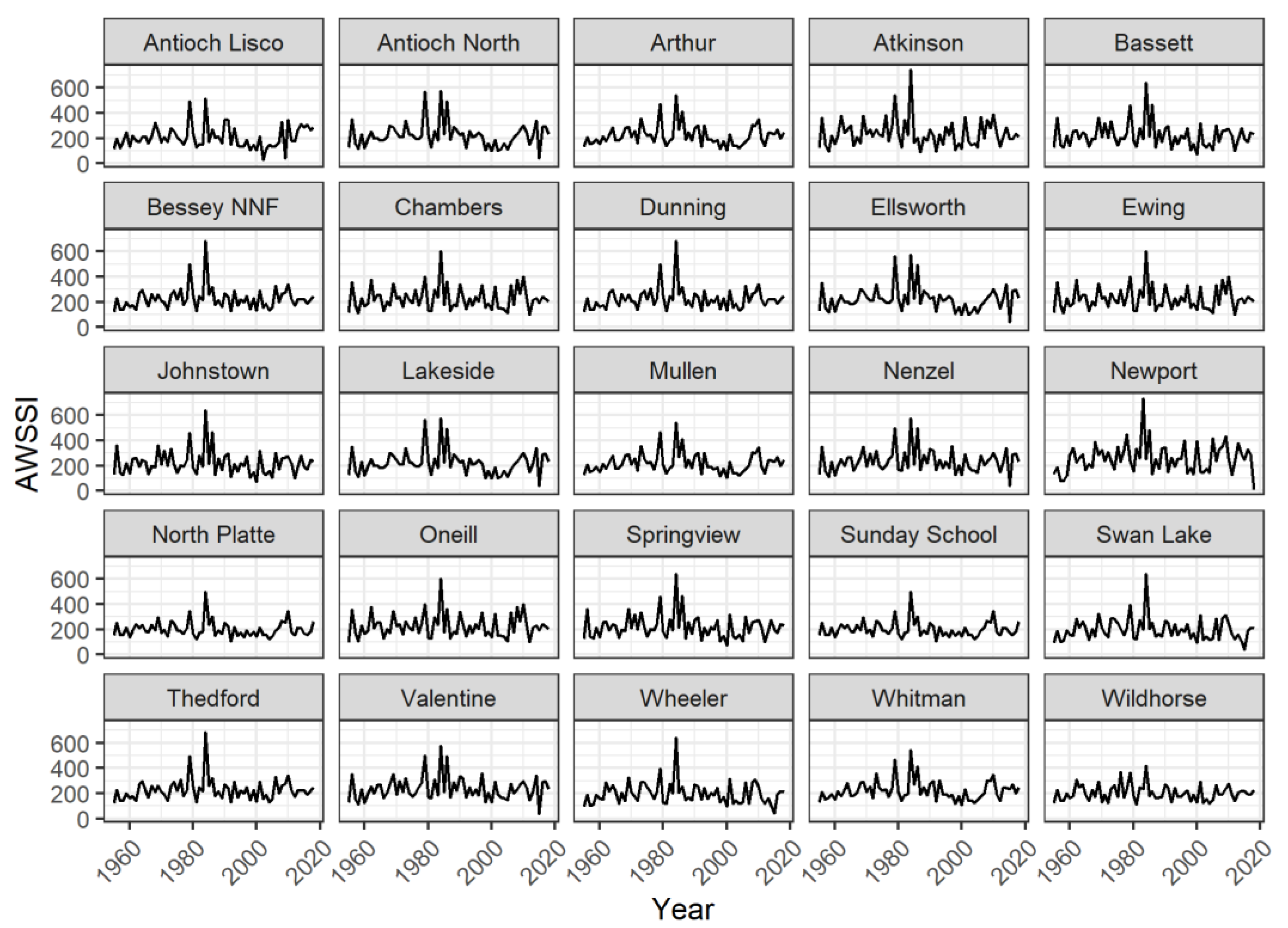
Deep snow can restrict prairie-grouse access to forage, while cold temperatures increase thermoregulatory demands, potentially creating energetic constraints during winter [55]. However, deep snow can also provide subnivean spaces that grouse species use to reduce thermoregulatory demands - a practice known as snow roosting [56]. We use the Accumulated Winter Season Severity Index (AWSSI) to evaluate relative, route-specific winter severity [57]. AWSSI uses temperature, precipitation and date thresholds to define the onset and cessation of winter. In the intervening period, a site accumulates daily points based on temperature, snowfall and snow depth that are totaled over the winter, producing a value that can be interpreted relative to data collected in other years at the same location. Large AWSSI values indicate more severe winters. We downloaded raw temperature and precipitation data from the Applied Climate Information System (ACIS) [58] database and calculated AWSSI scores for each site following the methods outlined in Boustead et al. (2015) [57]. If any climate data was missing for a portion of the time series, we used data from the next closest weather station (always less than 20 kms from the transect midpoint) to fill in the gap.
We also summarized climate data across the Sandhills by averaging annual values across monitoring sites.
2.4. Accounting for Missing Data
Unless otherwise specified for a metric, if data was missing at the beginning of the time series, we repeated the first observed value for all missing years. If data was missing from the end of a time series, we used the last observed value for all missing years. If data points were missing in the middle of a time series, we interpolated the missing value by taking the average of the year prior to and year following the missing data point. Our interpolation method assumes limited change in values at the beginning and end of a time series and local, linear relationships within the time series. To illustrate environmental trends, our primitive method of populating missing data is likely sufficient and allows for easy identification of observed data gaps through sequences of constant values. Prior to incorporating the environmental trends into an ecological analysis, we recommend using more sophisticated methods of data interpolation to avoid underestimating uncertainty and misidentifying relationships between predictor and response variables.
3. Results
We extracted environmental covariates at the finest spatial scale possible relative to the breeding ground survey routes with the goal of addressing drivers of prairie grouse population trends. However, the fine spatial scale necessary to study population drivers makes it challenging to pick out broader environmental trends in the Sandhills, one of our stated objectives. We include plots of data at the spatial scale covariates would enter a prairie grouse population model, as well as maps showing both the location and spatial extent of these fine scale covariates in Appendix A (Figure A1, Figure A2, Figure A3, Figure A4, Figure A5, Figure A6, Figure A7, Figure A8, Figure A9 and Figure A10). Below, we report summarized environmental trends across the Sandhills.
3.1. Hunting Pressure
Prairie grouse hunting pressure as captured by the number of hunter days in the field increased until the early 1980s and declined steadily thereafter (Figure 2). The minimum number of days in the field (7,489) occurred under highly restrictive regulations in the 1950s, with the maximum number of days in the field (89,797) coinciding with the height of the sport’s popularity in the 1980s. The mean number of hunter days in the field across years (n = 64) was 47,544 (sd = 20,011).
3.2. Birds of Prey
The average number of birds of prey per BBS route in the Sandhills has gradually increased since monitoring began in 1967 (Figure 3). The minimum number of birds per route was observed in 1985 (0.83) and the maximum in 2010 (5.46). Across years (n = 64), the mean number of birds per route was 2.09 (sd = 1.18).
3.3. Land Use Change
Crop production in the Sandhills rapidly increased between 1955 and 1960, plateaued until 2008, and declined thereafter (Figure 4). The lowest observed crop production in the Sandhills occurred in 1955 (215,906 hectares), with production peaking in 1984 (807,330 hectares). On average, 648,679 hectares of cropland are planted in the Sandhills each year (n = 64, sd = 138,078).
Hay production peaked in the Sandhills in the early 1960s (max = 965,363 hectares, 1962) and rapidly declined through 2020 (min = 384,280 hectares, 2015; Figure 4). Across years (n = 64), an average of 602,301 hectares were planted in hay (sd = 166,802).
CRP land enrollment did not begin until 1986 (min = 11,165 hectares, 1986), with acreage enrolled in the Sandhills reaching its apex in the early 1990s (max = 88,410 hectares, 1993-1994) and steadily declining through 2020 (Figure 4). Average CRP enrollment in the Sandhills is 29,198 hectares per year (n = 64, sd = 32,704).
3.4. Grazing Pressure
Grazing pressure in the Sandhills has increased since 1955, with minimum (1.33 AUMs/hectare) and maximum (2.25 AUMs/hectare) values occurring in the first and last year of the time series respectively (Figure 5). Across years (n = 64), the mean grazing pressure was 1.71 AUMs per hectare (sd = 0.25).
3.5. Climate
Drought conditions, as indexed by SCPDSI, have gradually increased in the Sandhills since 1955 (Figure 6). The lowest (most negative) drought index value (-3.61), indicating below average precipitation, was observed in 1955. The highest drought index value (3.66), indicating above average precipitation, occurred in 2010. Across years, the drought index averaged 0.037 with considerable variation between years (n = 64, sd = 1.52). Drought (negative SCPDSI) and non-drought (positive SCPDSI) years appeared with equal frequency across the time series.
Winter severity, as tracked by the AWSSI index, was highly variable between years, but the overall trend was relatively constant over time (Figure 6). The least severe winter in our time series occurred in 1955 (AWSSI = 123) and the most severe winter was observed in 1984 (AWSSI = 579). There is some indication that winters after 1990 are less severe than winters earlier in the time series (Figure 6). Across years, an average winter had observed AWSSI values of 222 (n = 64, sd = 76).
4. Discussion
We provide general guidance and a summary of resources to construct environmental covariates that can be paired with long-term species monitoring data pre-dating remotely-sensed habitat products. We then demonstrate our methodology for a 60+ year time series of breeding ground survey data from the Sandhills of Nebraska. While the Sandhills remain the largest intact grassland in the continental US, our results show that habitat quality has changed over time, even as quantity has remained relatively static. These changes may have shaped the differing population trajectories of prairie-chickens and sharp-tailed grouse. Given that we developed these covariates to explicitly model prairie grouse population drivers, an analysis beyond the scope of this manuscript, we minimize our speculation on how the environment may have produced separate population outcomes for prairie grouse species in our discussion. However, we address the likely consequences of long-term environmental trends in the Sandhills for grassland obligate species, like prairie grouse. In addition, we explore the challenges and limitations of repurposing long-term environmental monitoring data to construct biological covariates.
4.1. Risks—Hunting Pressure and Predation
While hunting pressure on small game species in the Sandhills has declined since the 1980s, populations of natural predators have increased. Less human predation on small game species may have increased prey availability for raptors, driving a numerical population response [59]. More likely, though, is that the ban on DDT in 1972, a pesticide that compromised bird of prey reproduction, combined with land use change and additional protections against harvest under the Migratory Bird Treaty Act, led raptor populations to flourish [60,61]. The development of agricultural, transportation, and energy infrastructure has increased the prevalence of edge habitat, nesting and perching structures [62], and the abundance of small mammal prey [63] in the Sandhills. In addition, woody encroachment into grassland habitat, a major threat to the eastern Sandhills [64,65], provides nesting and perching substrates for raptors [66]. Given that human harvest of small game is thought to be a compensatory source of mortality [67,68], while raptor predation is potentially additive [69,70], overall predation risk in the Sandhills has likely increased since 1955 for both small game and non-game species.
4.2. Resources—Land Use Change
Agricultural practices in the Sandhills have changed since the 1950s with a shift from predominantly hay to crop production. Cropland has less habitat value for wildlife than hayfields because crops are often sparsely-planted monocultures, reliant on intensive irrigation, herbicide and pesticide use, and when harvested leave bare ground or stubble for portions of the year [71]. From the perspective of cover for wildlife, cropland constitutes habitat loss. However, some species, like deer, waterfowl, turkeys and prairie-chickens use waste grain as a high energy food source, especially during the resource-limited winter months [55,72]. Given that less than 5% of the land area of the Sandhills is used for crop production [73], it is possible that the benefit of additional food resources outweighs the loss of cover.
Some cropland area was converted back to grassland through the CRP program, although enrollment declined with price increases of agricultural commodities [74]. At the height of the program, acreage reclaimed as grassland was less than 10% of acreage converted to cropland during the same period. CRP plantings provide more habitat value for wildlife than cultivated acres [71]. However, non-native grass seed mixes and high seeding densities used in portions of the Sandhills [75] may have resulted in lower quality grassland habitat relative to native range.
Presently, there are more cultivated acres in the Sandhills than in 1955, which translates into an overall loss of untouched grassland habitat and resources for most wildlife species. Yet, alternative land uses including cropland, hay and CRP, provide some habitat value for wildlife.
4.3. Conditions—Grazing Pressure
Grazing pressure has increased in the Sandhills since 1955, through a combination of increased cattle size and the number of animals on pasture. Whereas the Sandhills is grazed conservatively relative to other grassland systems because of the unstable, sandy soil, the ubiquity of grazing means almost all wildlife habitat is shared with cattle [10,73]. Increased cattle demand for forage biomass means less vegetation on the landscape to provide food and cover for wildlife. However, at intermediate levels of grazing pressure, cattle may increase habitat heterogeneity, improving habitat quality for some wildlife species [39]. The effects of grazing interact with variation in the climate and underlying habitat [39]. For example, the Sandhills follow both east-to-west precipitation and vegetation gradients [10]. Greater rainfall in the eastern Sandhills supports tallgrass prairie vegetation, while the western Sandhills are characterized by semi-arid short grass prairie [10]. Increased grazing pressure likely has a greater impact in the western Sandhills where vegetation is already sparse and may be further exacerbated by the increasing frequency of drought conditions [76].
The Sandhills’ value as rangeland is largely what keeps it an intact grassland system, though. A reduction in grazing pressure would likely lead to some lands being developed for economic activities less favorable to wildlife. Yet, ranchers should be aware that they are collectively asking more of the Sandhills to support cattle than ever before. Despite the importance of grazing in the Sandhills, here we present the first longitudinal, private-land grazing index for the system, building on the work of Cumming et al. (2019) [42]. We hope that by providing a tool to quantify grazing demand relative to available pastureland we can help ranchers maintain a landscape that meets both the needs of cattle and wildlife.
4.4. Conditions—Climate
Over the past 60 years, the Sandhills have entered a state of persistent drought during the growing season, while winters have also decreased in severity. The landscape is becoming drier, which has negative consequences for vegetation productivity [77]. Less vegetation on the landscape limits food and cover for wildlife. When coupled with increased grazing demand for forage, the shifting climate is likely intensifying competition between cattle and wildlife for resources. Unfortunately, our pastureland acreage proxy for forage supply does not capture how grassland productivity on those acres may change over time. However, newer remotely sensed products, like herbaceous biomass on the Rangeland Analysis Platform [78,79,80] provide insight into how productivity in the Sandhills has changed in more recent years. And while decreasing winter severity may result in lower overwinter mortality from severe weather events, it exacerbates drought conditions. In addition, wildlife entering winter in poor condition because of limited food availability due to drought may be less able to tolerate even mild conditions [55,81]. Overall, the combination of increased grazing pressure, drought, and less severe winters have likely resulted in environmental conditions that are less favorable to wildlife than 60 years ago.
4.5. Environmental Change
Trends of increased predation risk, decreased resource availability, and more extreme environmental conditions have likely resulted in decreased habitat quality for most grassland obligate species of wildlife in the Sandhills over the past 60 years. Even though the Sandhills remain a largely intact grassland landscape, resource managers should be aware that documented changes in habitat quality may also be of concern for species’ persistence. Knowledge of habitat change coupled with basic understanding of species’ biology can also help managers identify which wildlife may warrant additional monitoring. However, environmental change, particularly slow change over a prolonged period of time, is not universally bad for wildlife. In our focused exploration of prairie grouse, we found that prairie chicken populations increased over the past 60 years. In addition, as we quantified prairie grouse population drivers, we also saw that bird of prey populations increased. Changes in habitat quality may bring about future shifts in species’ composition and relative abundance in the Sandhills as novel environmental conditions redefine traits that maximize fitness.
4.6. Limitations of Our Approach
Repurposing long-term environmental monitoring data as covariates in ecological models focused on particular species is not without challenges, as we are often going beyond the data’s intended use-case. First, repurposed data may not represent dimensions of the environment in ways that capture relevant species’ biology. For example, our AWSSI winter severity index provides an anthropocentric representation of winter severity. AWSSI penalizes any snow depth, which may capture the snow effects on most wildlife species, but does not adequately describe prairie grouse interactions with snow. In deep snow, prairie grouse can use subnivean environments to aid in thermoregulation [33]. An ideal winter severity index for prairie grouse would penalize snow depths too shallow to facilitate snow roosting but treat deep snow as beneficial when coupled with extreme cold temperatures. When repurposing data, we recommend carefully evaluating how species’ biology aligns with the considered environmental metrics. Covariate data may need to be modified to better reflect species’ interactions with their environment or different data sources considered altogether.
The spatiotemporal scale of the environmental data relative to historical species’ monitoring may also limit the data’s utility when addressing ecological questions. Because environmental monitoring pre-dating remote sensing was reliant on human labor rather than technology, data was collected less frequently and at coarser spatial scales. Low spatiotemporal resolution environmental covariates are likely adequate when species’ monitoring data is also collected or aggregated to coarse spatiotemporal scales. Longer time series of data can also be useful to detect environmental effects when the native spatiotemporal resolution of the monitoring or covariate data insufficiently captures finer-scale variation. When repurposing data, we recommend evaluating the scale of the environmental covariates relative to the species’ monitoring data to determine if the spatiotemporal resolution is sufficient to address the proposed question.
As in our example, covariates intended for the same model may have a variety of spatiotemporal resolutions. Covariates with finer spatiotemporal resolution can capture more variation across space and time, potentially giving them more explanatory power. If covariates with fine spatiotemporal resolutions consistently have larger effect sizes or are highly ranked by model selection approaches, we caution that statistical importance may reflect scale rather than biology. While we recommend scaling covariate data as closely as possible to the biological process it is meant to represent, if high resolution covariates consistently dominate models, upscaling covariates to match the coarsest resolution may be necessary.
5. Conclusions
We provide guidance and resources for practitioners that want to construct environmental covariates to pair with historical monitoring data that pre-date remote-sensing technologies. Whereas our workflow emphasizes wildlife monitoring data, our approach is generalizable to historical monitoring data collected in fields like fisheries, forestry, agronomy, anthropology, and urban planning. In addition to serving as model covariates, longitudinal summaries of environmental monitoring data provide insight into environmental change. Here, we show that although the Sandhills remain an intact grassland ecosystem, habitat quality for grassland obligate species has changed over time. Since 1955, risks to many grassland obligate species, like prairie grouse, have increased, resource availability has declined, and climatic conditions have become less favorable. Some covariates may also have application beyond their intended use in an ecological model. For example, our longitudinal private land grazing metric is the first spatially-explicit representation of how grazing pressure has changed over time in the Sandhills. Knowledge of trends in grazing intensity are useful to livestock producers, land-use planners, and natural resources managers alike. We hope that by providing preliminary guidance and a summary of historical environmental data that we have encouraged wildlife practitioners to find new value in old species’ monitoring data for addressing questions of modern-day conservation concern.
Author Contributions
Conceptualization, D.J.B., L.A.P. and J.P.C.; methodology, D.J.B., J.J.L., L.A.P., J.P.C., W.S. and J.P.; software, D.J.B.; validation, D.J.B., L.A.P. and J.P.C.; formal analysis, D.J.B.; investigation, D.J.B.; resources, J.J.L., L.A.P. and J.P.C.; data curation, D.J.B.; writing—original draft preparation, D.J.B.; writing—review and editing, D.J.B., J.J.L., L.A.P. and J.P.C.,; visualization, D.J.B.; supervision, J.J.L., L.A.P. and J.P.C.; project administration, J.J.L., L.A.P. and J.P.C.; funding acquisition, L.A.P. and J.P.C. All authors have read and agreed to the published version of the manuscript.
Funding
The data compilation and analyses received no external funding, and D.J.B. was supported by the School of Natural Resources.
Data Availability Statement
All data used in this manuscript is publicly available with sources cited in the text and links to each source embedded in the citations.
Acknowledgments
Thank you to the numerous employees and members of international, federal, and state agencies, ecological research networks and observatories, universities, and conservation organizations that collected and archived the data used in this manuscript. Your foresight and dedication to environmental monitoring and conservation made this analysis possible.
Conflicts of Interest
The authors declare no conflicts of interest.
Appendix A
Figure A1.
Raptor predation pressure index regions in the Sandhills of Nebraska, USA. Counties whose Breeding Bird Survey (BBS) routes were included in the Western Region are shaded in blue. Counties in the Eastern Region are colored purple.
Figure A1.
Raptor predation pressure index regions in the Sandhills of Nebraska, USA. Counties whose Breeding Bird Survey (BBS) routes were included in the Western Region are shaded in blue. Counties in the Eastern Region are colored purple.
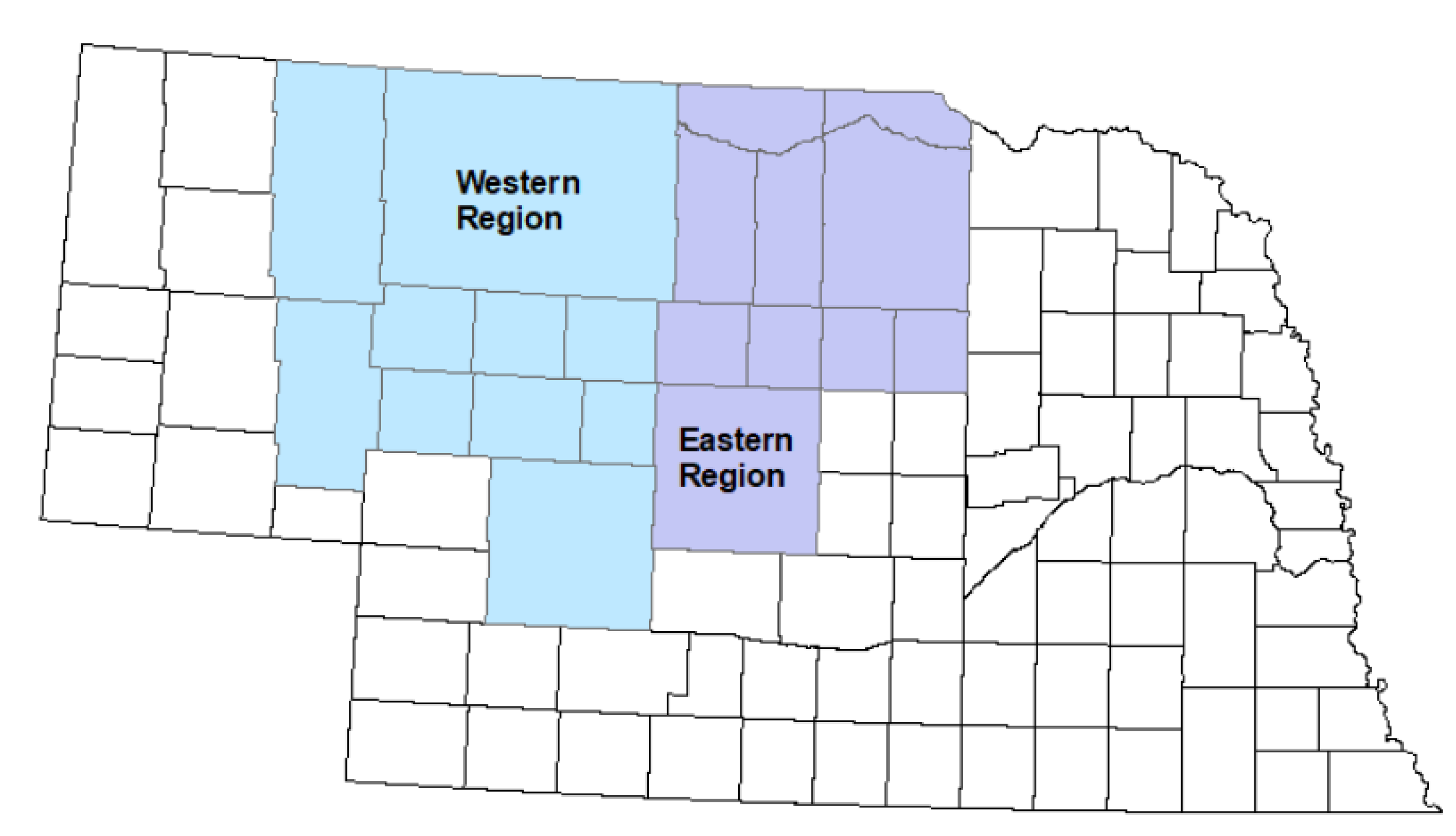
Figure A2.
Mean number of raptors per BBS route from 1955-2018, for the Eastern and Western Regions of the Sandhills of Nebraska, USA. Data taken from BBS (1966-2019).
Figure A2.
Mean number of raptors per BBS route from 1955-2018, for the Eastern and Western Regions of the Sandhills of Nebraska, USA. Data taken from BBS (1966-2019).

Figure A3.
Grazing region in the Sandhills of Nebraska, USA. Counties in the Sheridan-Garden region are shaded in green. Counties in the Sandhills region are depicted in blue. North Central region counties are pink. Custer region counties are light orange.
Figure A3.
Grazing region in the Sandhills of Nebraska, USA. Counties in the Sheridan-Garden region are shaded in green. Counties in the Sandhills region are depicted in blue. North Central region counties are pink. Custer region counties are light orange.
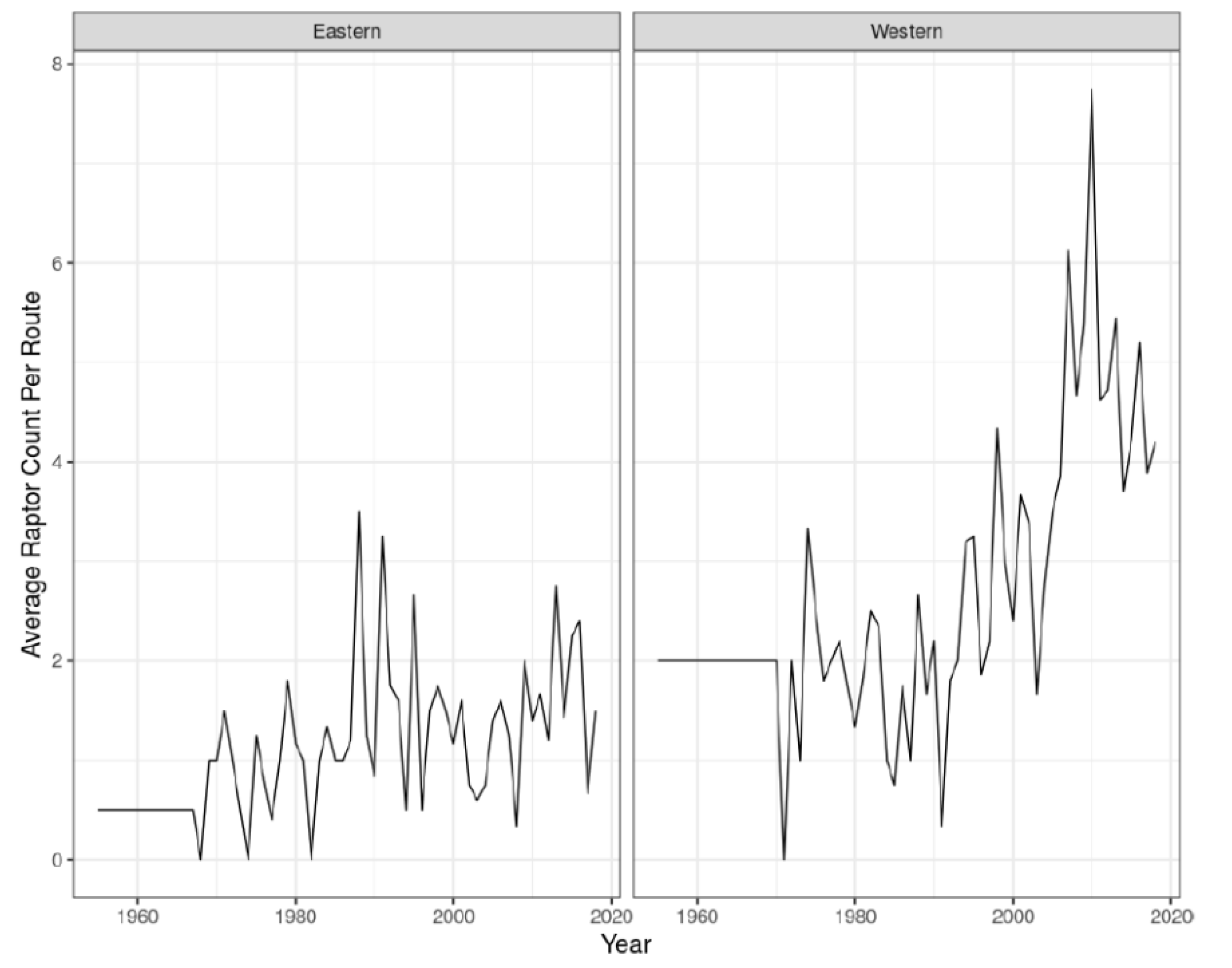
Figure A4.
Annual stocking rate (AUMs/hectare) from 1955-2018 for four different grazing regions within the Sandhills of Nebraska, USA. Base data from USDA NASS (2026b).
Figure A4.
Annual stocking rate (AUMs/hectare) from 1955-2018 for four different grazing regions within the Sandhills of Nebraska, USA. Base data from USDA NASS (2026b).
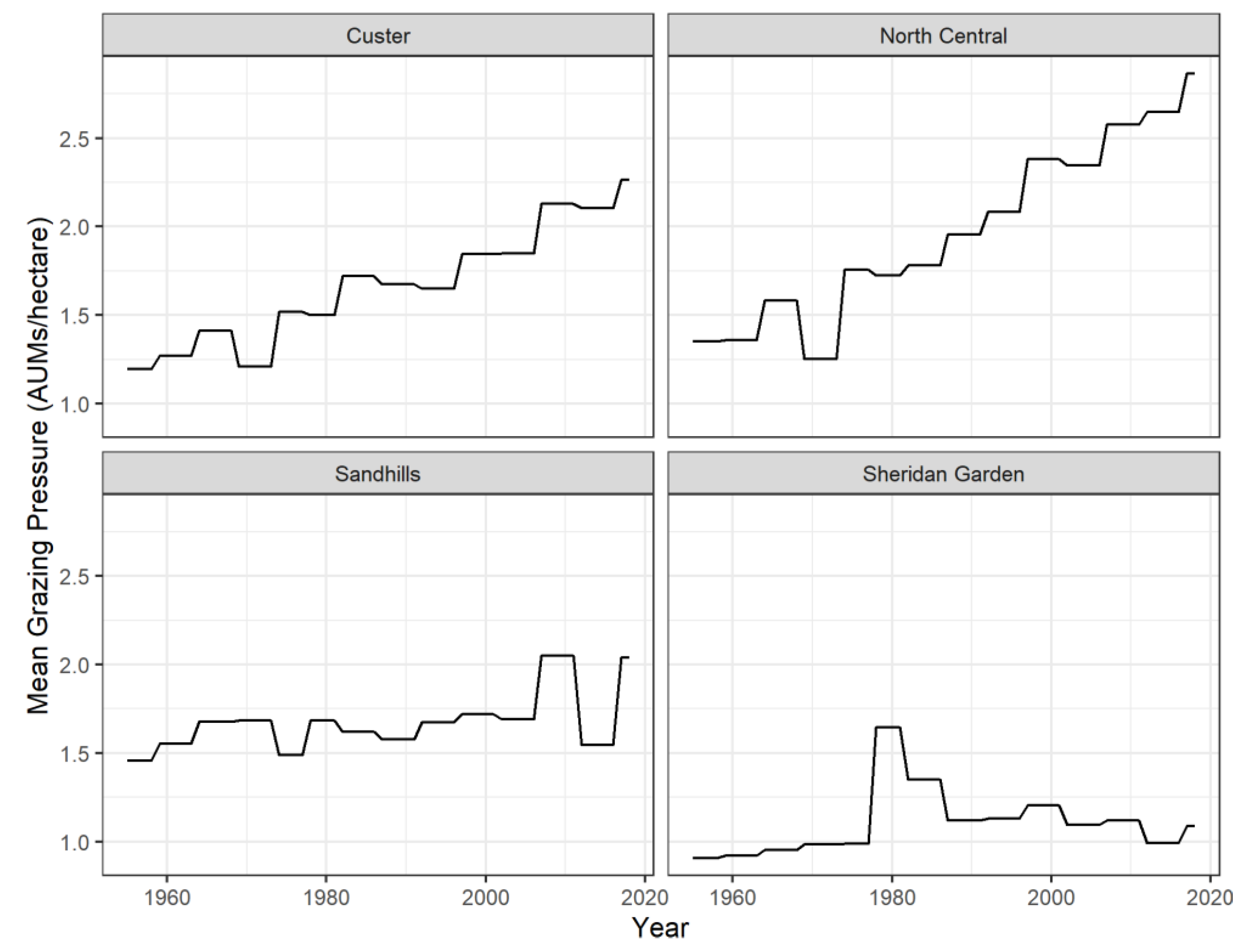
Figure A5.
Sandhills counties with prairie grouse breeding ground survey routes included in cropland, hay, and Conservation Reserve Program (CRP) land use change estimates, Nebraska, USA.
Figure A5.
Sandhills counties with prairie grouse breeding ground survey routes included in cropland, hay, and Conservation Reserve Program (CRP) land use change estimates, Nebraska, USA.
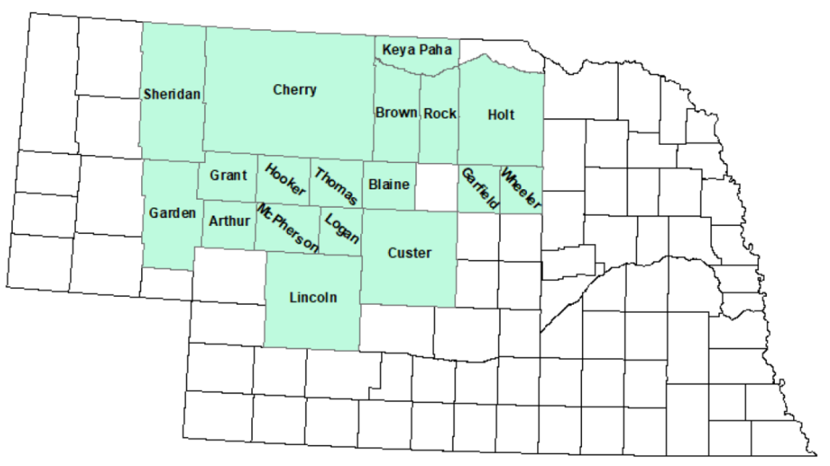
Figure A6.
Cropland acreage by county from 1955-2018 in the Sandhills of Nebraska, USA. Data from NASS (2026a).
Figure A6.
Cropland acreage by county from 1955-2018 in the Sandhills of Nebraska, USA. Data from NASS (2026a).
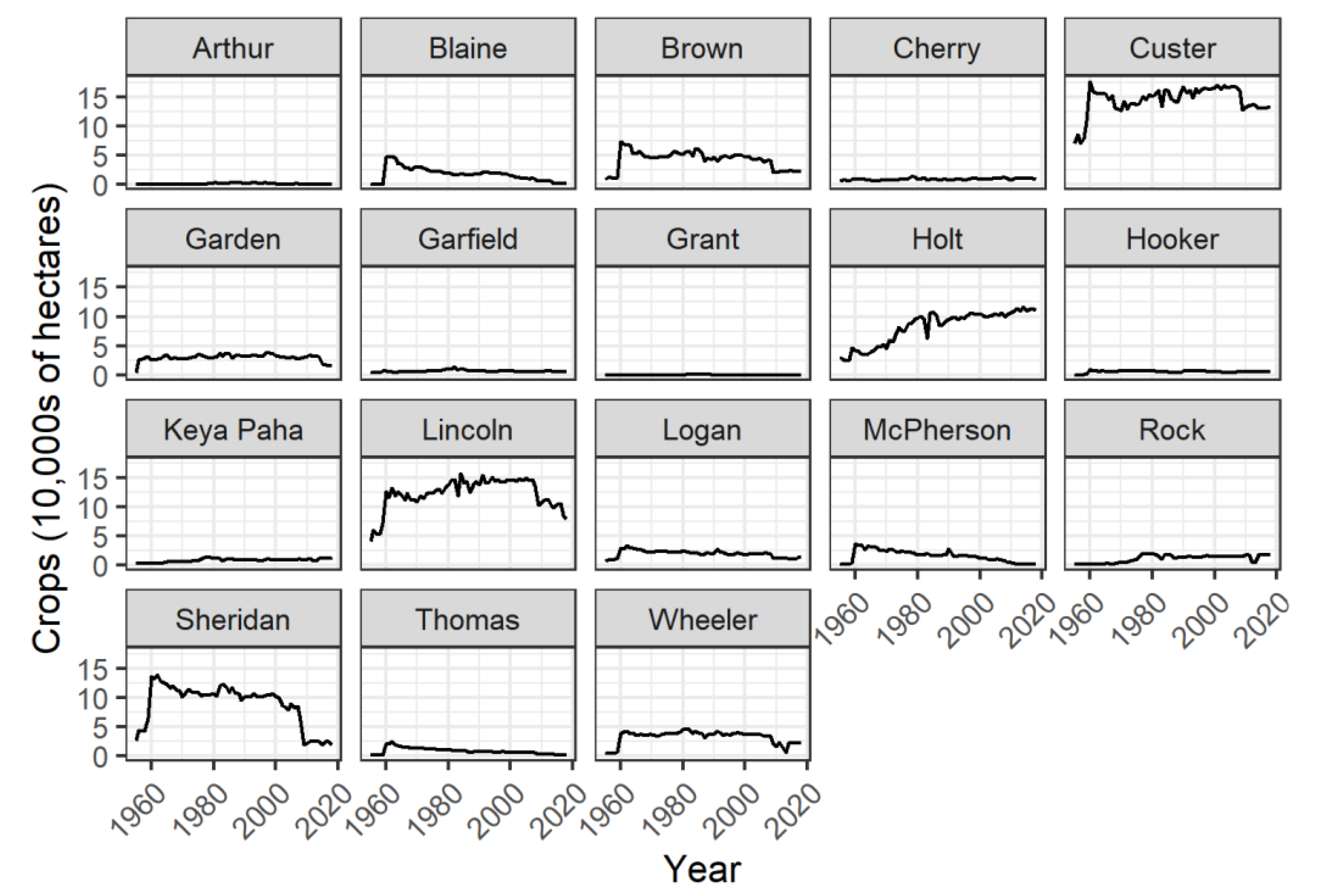
Figure A7.
Hay acreage by county from 1955-2018 in the Sandhills of Nebraska, USA. Data from NASS (2026a).
Figure A7.
Hay acreage by county from 1955-2018 in the Sandhills of Nebraska, USA. Data from NASS (2026a).
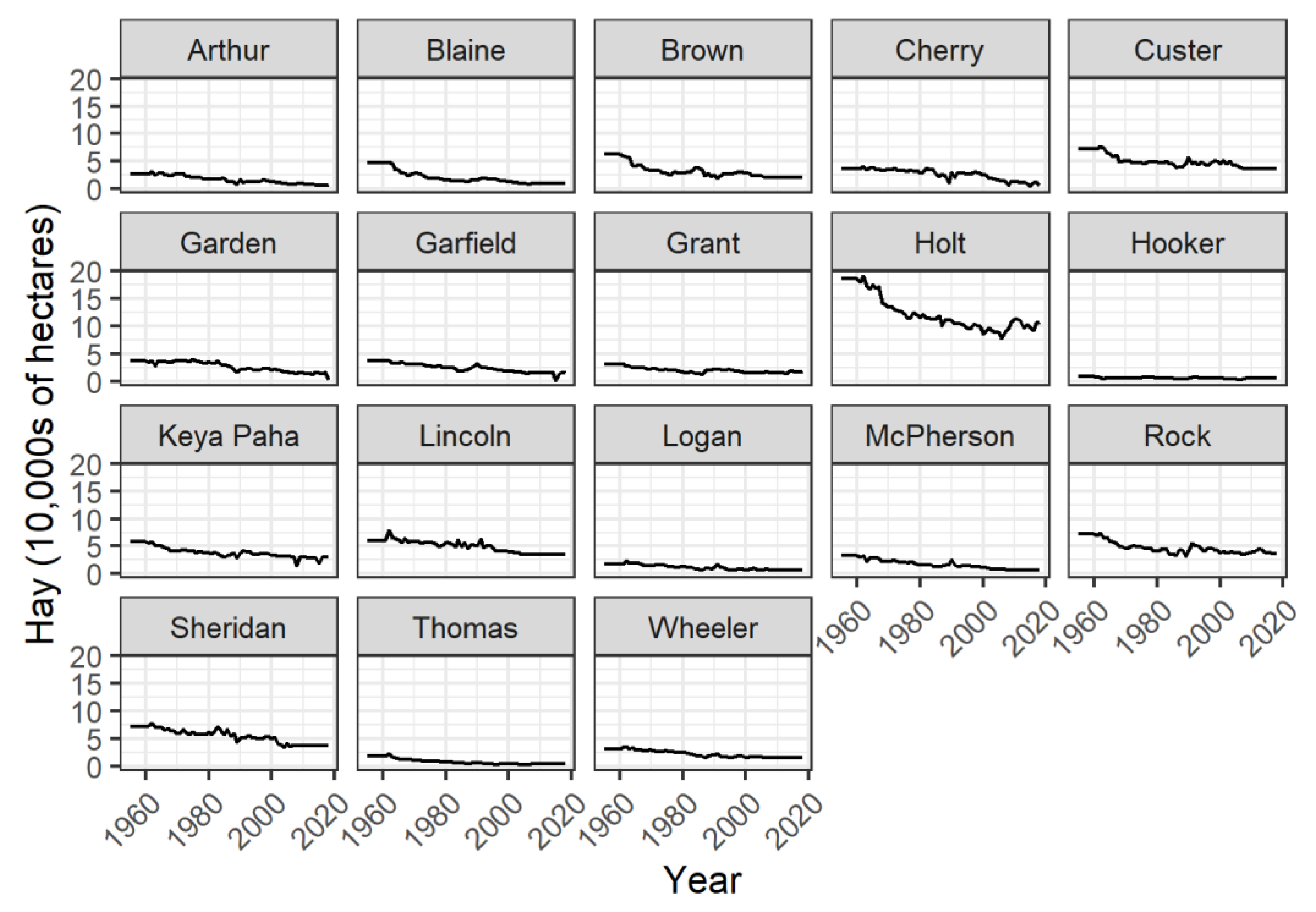
Figure A8.
Conservation Reserve Program (CRP) acreage by county from 1955-2018 in the Sandhills of Nebraska, USA. Data from USDA (2026).
Figure A8.
Conservation Reserve Program (CRP) acreage by county from 1955-2018 in the Sandhills of Nebraska, USA. Data from USDA (2026).
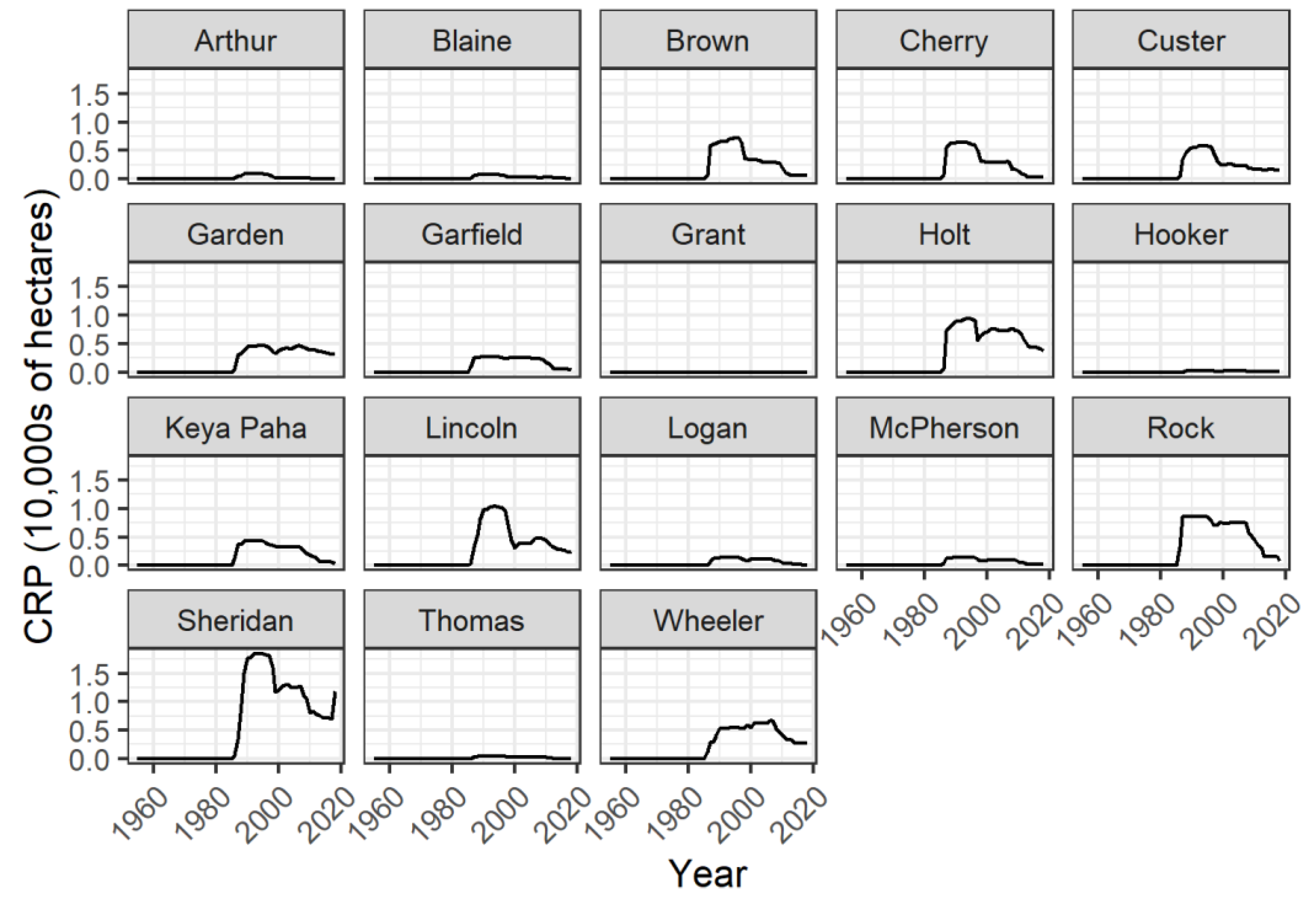
Figure A9.
Self-Calibrating Palmer Drought Severity Index (SCPDSI) values by breeding ground survey route from 1955-2018 in the Sandhills of Nebraska, USA. Larger (non-negative) values indicate a decrease in drought conditions relative to a local baseline. Data from NDMC (2026).
Figure A9.
Self-Calibrating Palmer Drought Severity Index (SCPDSI) values by breeding ground survey route from 1955-2018 in the Sandhills of Nebraska, USA. Larger (non-negative) values indicate a decrease in drought conditions relative to a local baseline. Data from NDMC (2026).
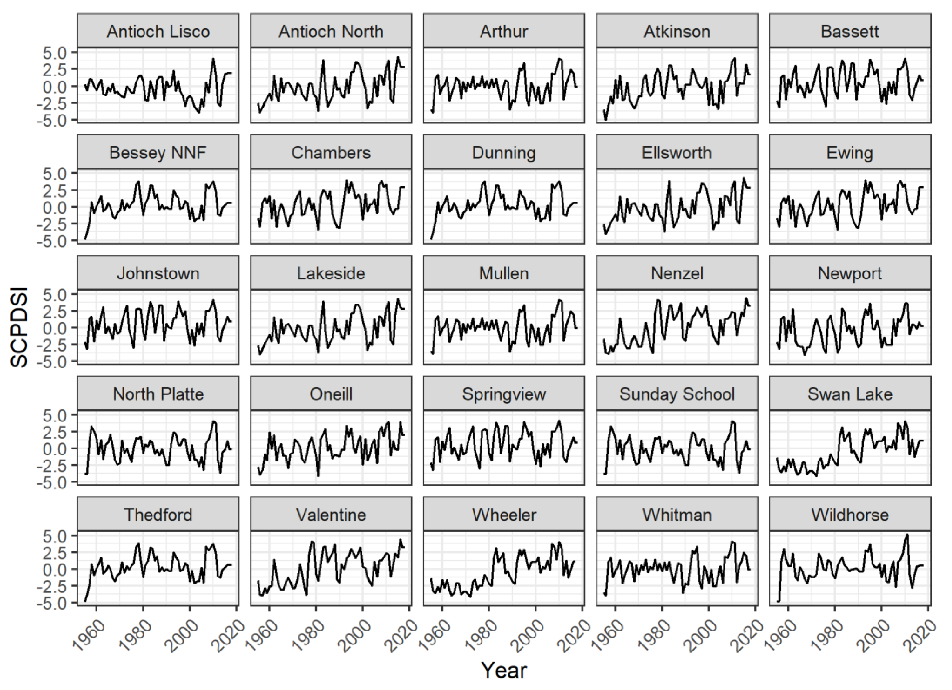
Figure A10.
Accumulated Winter Season Severity Index (AWSSI) values by route from 1955-2018 in the Sandhills of Nebraska, USA. Larger (non-negative) values indicate an increase in winter severity. Data from ACIS (2026).
Figure A10.
Accumulated Winter Season Severity Index (AWSSI) values by route from 1955-2018 in the Sandhills of Nebraska, USA. Larger (non-negative) values indicate an increase in winter severity. Data from ACIS (2026).
References
- Krauss, J.; Bommarco, R.; Guardiola, M.; Heikkinen, R.K.; Helm, A.; Kuussaari, M.; Lindborg, R.; Öckinger, E.; Pärtel, M.; Pino, J.; et al. Habitat Fragmentation Causes Immediate and Time-Delayed Biodiversity Loss at Different Trophic Levels. Ecol. Lett. 2010, 13, 597–605. [Google Scholar] [CrossRef] [PubMed]
- Cornford, R.; Spooner, F.; McRae, L.; Purvis, A.; Freeman, R. Ongoing Over-Exploitation and Delayed Responses to Environmental Change Highlight the Urgency for Action to Promote Vertebrate Recoveries by 2030. Proc. Biol. Sci. 290, 20230464. [CrossRef] [PubMed]
- Semper-Pascual, A.; Burton, C.; Baumann, M.; Decarre, J.; Gavier-Pizarro, G.; Gómez-Valencia, B.; Macchi, L.; Mastrangelo, M.E.; Pötzschner, F.; Zelaya, P.V.; et al. How Do Habitat Amount and Habitat Fragmentation Drive Time-Delayed Responses of Biodiversity to Land-Use Change? Proc. Biol. Sci. 2021, 288, 20202466. [Google Scholar] [CrossRef] [PubMed]
- Berger, D.J.; Lusk, J.J.; Powell, L.A.; Carroll, J.P. Exploring Old Data with New Tricks: Long-Term Monitoring Indicates Spatial and Temporal Changes in Populations of Sympatric Prairie Grouse in the Nebraska Sandhills. Diversity 2023, 15, 114. [Google Scholar] [CrossRef]
- Storch, I. Conservation Status of Grouse Worldwide: An Update. Wildl. Biol. 2007, 13, 5–12. [Google Scholar] [CrossRef]
- Svedarsky, W.D.; Westemeier, R.L.; Robel, R.J.; Gough, S.; Toepher, J.E. Status and Management of the Greater Prairie-Chicken Tympanuchus Cupido Pinnatus in North America. Wildl. Biol. 2000, 6, 277–284. [Google Scholar] [CrossRef]
- Shuai, H.; Hu, J.; Zheng, S.; Ma, Z.; Liu, J. Most Bird Species Remain Poorly Studied but Threated Status Promotes Research Effort. Avian Res. 2024, 15, 100215. [Google Scholar] [CrossRef]
- Anderson, L.C.; Powell, L.A.; Schacht, W.H.; Lusk, J.J.; Vodehnal, W.L. Greater Prairie-Chicken Brood-Site Selection and Survival in the Nebraska Sandhills. J. Wildl. Manag. 2015, 79, 559–569. [Google Scholar] [CrossRef]
- King, K.C.; Caven, A.J.; Geluso, K. Lekking Behavior of a Sharp-Tailed Grouse in South-Central Nebraska. Prairie Nat. 2018, 50. [Google Scholar]
- Bleed, A.S.; Flowerday, C.A. An Atlas of the Sand Hills; Conservation and Survey Division, Institute of Agriculture and Natural Resources; University of Nebraska-Lincoln: Lincoln, USA, 1989. [Google Scholar]
- Lark, T.J.; Meghan Salmon, J.; Gibbs, H.K. Cropland Expansion Outpaces Agricultural and Biofuel Policies in the United States. Environ. Res. Lett. 2015, 10, 044003. [Google Scholar] [CrossRef]
- Wright, C.K.; Wimberly, M.C. Recent Land Use Change in the Western Corn Belt Threatens Grasslands and Wetlands. Proc. Natl. Acad. Sci. U S A 2013, 110, 4134–4139. [Google Scholar] [CrossRef] [PubMed]
- Sylvester, K.M.; Brown, D.G.; Deane, G.D.; Kornak, R.N. Land Transitions in the American Plains: Multilevel Modeling of Drivers of Grassland Conversion (1950 to 2000). Agric. Ecosyst. Environ. 2013, 168, 7–15. [Google Scholar] [CrossRef] [PubMed]
- Theobald, D. Landscape Patterns of Exurban Growth in the USA from 1980 to 2020. Ecol. Soc. 2005, 10. [Google Scholar] [CrossRef]
- Baynard, C.W.; Mjachina, K.; Richardson, R.D.; Schupp, R.W.; Lambert, J.D.; Chibilyev, A.A. Energy Development in Colorado’s Pawnee National Grasslands: Mapping and Measuring the Disturbance Footprint of Renewables and Non-Renewables. Environ. Manag. 2017, 59, 995–1016. [Google Scholar] [CrossRef] [PubMed]
- Ott, J.P.; Hanberry, B.B.; Khalil, M.; Paschke, M.W.; Post van der Burg, M.; Prenni, A.J. Energy Development and Production in the Great Plains: Implications and Mitigation Opportunities. Rangel. Ecol. Manag. 2021, 78, 257–272. [Google Scholar] [CrossRef]
- Allred, B.W.; Smith, W.K.; Twidwell, D.; Haggerty, J.H.; Running, S.W.; Naugle, D.E.; Fuhlendorf, S.D. Ecosystem Services Lost to Oil and Gas in North America. Science 2015, 348, 401–402. [Google Scholar] [CrossRef] [PubMed]
- Burda, B.; Somers, C.M.; Conkin, K.; Fisher, R.J. Lek Habitat Suitability for the Sharp-Tailed Grouse (Tympanuchus Phasianellus Jamesi) on the Northern Great Plains. PLoS ONE 2022, 17, e0265316. [Google Scholar] [CrossRef] [PubMed]
- Poiani, K.A.; Merrill, M.D.; Chapman, K.A. Identifying Conservation-Priority Areas in a Fragmented Minnesota Landscape Based on the Umbrella Species Concept and Selection of Large Patches of Natural Vegetation. Conserv. Biol. 2001, 15, 513–522. [Google Scholar] [CrossRef]
- McNew, L.B.; Winder, V.L.; Pitman, J.C.; Sandercock, B.K. Alternative Rangeland Management Strategies and the Nesting Ecology of Greater Prairie-Chickens. Rangel. Ecol. Manag. 2015, 68, 298–304. [Google Scholar] [CrossRef]
- Hardy, M.A.; Broadway, M.S.; Pollentier, C.D.; Radeloff, V.C.; Riddle, J.D.; Hull, S.D.; Zuckerberg, B. Responses to Land Cover and Grassland Management Vary across Life-History Stages for a Grassland Specialist. Ecol. Evol. 2020, 10, 12777–12791. [Google Scholar] [CrossRef] [PubMed]
- Matthiopoulos, J.; Fieberg, J.; Aarts, G.; Beyer, H.L.; Morales, J.M.; Haydon, D.T. Establishing the Link between Habitat Selection and Animal Population Dynamics. Ecol. Monogr. 2015, 85, 413–436. [Google Scholar] [CrossRef]
- Wilhite, D.A.; Hubbard, K.G. Climate. In An Atlas of the Sand Hills; University of Nebraska: Conservation and Survey Division: Lincoln, NE, USA, 1989; pp. 17–28. [Google Scholar]
- Whitcomb, R.F. Nebraska Sand Hills: The Last Prairie. Proc. Proc. North Am. Prairie Conf. 1989, Vol. 33, 57–69. [Google Scholar]
- Powell, L.A.; Schacht, W.H.; Anderson, L.C.; Vodehnal, L.W. Management of Sandhills Rangelands for Greater Prairie-Chickens. In University of Nebraska Extension Circular; University of Nebraska-Lincoln: Lincoln, Nebraska, USA, 2014. [Google Scholar]
- Miller, S.M. Land Development and Use. In An Atlas of the Sand Hills; Bleed, Flowerday, C., Eds.; Institute of Agricultural and Natural Resources, University of Nebraska-Lincoln: Lincoln, USA, 1989; pp. 207–226. [Google Scholar]
- Burham, K.P.; Anderson, D.R. Tests of Compensatory vs. Additive Hypotheses of Mortality in Mallards. Ecology 1984, 65, 105–112. [Google Scholar] [CrossRef]
- Schroeder, M.A.; Baydack, R.K. Predation and the Management of Prairie Grouse. Wildl. Soc. Bull. 2001, 29, 24–32. [Google Scholar]
- Pardieck, K.L.; Ziolkowski, D.J.; Lutmerding, M.; Aponte, V.I.; Hudson, M.A.R. North American Breeding Bird Survey Dataset 1966 - 2019: U.S. Geological Survey Data Release 2020. [PubMed]
- Vodehnal, W.L. Status and Management of the Greater Prairie-Chicken in Nebraska 1999. [PubMed]
- Sisson, L. The Sharp-Tailed Grouse in Nebraska; Nebraska Game and Parks Commission: Lincoln, USA, 1976. [Google Scholar]
- Hiller, T.L.; McFadden, J.E.; Powell, L.A.; Schacht, W.H. Seasonal and Interspecific Landscape Use of Sympatric Greater Prairie-Chickens and Plains Sharp-Tailed Grouse. Wildl. Soc. Bull. 2019, 43, 244–255. [Google Scholar] [CrossRef]
- Svedarsky, W.D.; Toepher, J.E.; Westemeier, R.L.; Robel, R.J.; Igl, L.D.; Shaffer, J.A. The Effects of Management Practices on Grassland Birds - Greater Prairie-Chicken (Tympanuchus Cupido Pinnatus); US Geological Survey Professional Paper, 2022. [Google Scholar]
- Rodgers, R.W.; Hoffman, R.W. Prairie Grouse Population Response to CRP Grasslands: An Overview. In The conservation reserve program - planting for the future: proceedings of a national conference; U.S. Geological Survey, Biological Resources Discipline, Scientific Investigations Report 2005-5145: Fort Collins, Colorado, USA, 2005; pp. 120–128. [Google Scholar]
- USDA National Agricultural Statistics Service (NASS) Quick Stats 2020.
- Powell, J.; Martin, B.; Dreitz, V.J.; Allred, B.W. Grazing Preferences and Vegetation Feedbacks of the Fire-Grazing Interaction in the Northern Great Plains. Rangel. Ecol. Manag. 2018, 71, 45–52. [Google Scholar] [CrossRef]
- Horton, J.R.; Roy, C.L.; Haus, J.M.; Hiller, B.J. Greater Prairie-Chicken Nest Survival and Changes in Vegetation Structure and Composition with Conservation Grazing. Wildl. Soc. Bull. 2025, 49, e1601. [Google Scholar] [CrossRef]
- Milligan, M.C.; Berkeley, L.I.; McNew, L.B. Habitat Selection of Female Sharp-Tailed Grouse in Grasslands Managed for Livestock Production. PLoS ONE 2020, 15, e0233756. [Google Scholar] [CrossRef] [PubMed]
- Fritts, S.R.; Grisham, B.A.; Cox, R.D.; Boal, C.W.; Haukos, D.A.; McDaniel, P.; Hagen, C.A.; Greene, D.U. Interactive Effects of Severe Drought and Grazing on the Life History Cycle of a Bioindicator Species. Ecol. Evol. 2018, 8, 9550–9562. [Google Scholar] [CrossRef] [PubMed]
- Winder, V.L.; McNew, L.B.; Pitman, J.C.; Sandercock, B.K. Effects of Rangeland Management on Survival of Female Greater Prairie-Chickens. J. Wildl. Manag. 2018, 82, 113–122. [Google Scholar] [CrossRef]
- USDA National Agricultural Statistics Service (NASS) Census of Agriculture 2020.
- Cumming, K.; Parsons, J.; Schacht, W.H.; Baskerville, B. Examining the Capacity of Nebraska Rangelands for Cattle Production. West. Econ. Forum 2019, 17, 46–61. [Google Scholar]
- Linden, D.R.; Titgemeyer, E.C.; Olson, K.C.; Anderson, D.E. Effects of Gestation and Lactation on Forage Intake, Digestion, and Passage Rates of Primiparous Beef Heifers and Multiparous Beef Cows. J. Anim. Sci. 2014, 92, 2141–2151. [Google Scholar] [CrossRef] [PubMed]
- Grings, E.E.; Short, R.E.; MacNeil, M.D.; Haferkamp, M.R.; Adams, D.C. Efficiency of Production in Cattle of Two Growth Potentials on Northern Great Plains Rangelands during Spring-Summer Grazing. J. Anim. Sci. 1996, 74, 2317–2326. [Google Scholar] [CrossRef] [PubMed]
- McMurry, B. Beef Magazine. 2009. [Google Scholar] [CrossRef]
- Lautenbach, J.M.; Haukos, D.A.; Sullins, D.S.; Hagen, C.A.; Lautenbach, J.D.; Pitman, J.C.; Plumb, R.T.; Robinson, S.G.; Kraft, J.D. Factors Influencing Nesting Ecology of Lesser Prairie-Chickens. J. Wildl. Manag. 2019, 83, 205–215. [Google Scholar] [CrossRef]
- Earl, J.E.; Fuhlendorf, S.D. Relative Importance of Climate Variables to Population Vital Rates: A Quantitative Synthesis for the Lesser Prairie-Chicken. PLoS ONE 2016, 11, e0163585. [Google Scholar] [CrossRef] [PubMed]
- Newell, F.L.; Ausprey, I.J.; Robinson, S.K. Wet and Dry Extremes Reduce Arthropod Biomass Independently of Leaf Phenology in the Wet Tropics. Glob. Chang Biol. 2023, 29, 308–323. [Google Scholar] [CrossRef] [PubMed]
- Morrow, M.E.; Chester, R.E.; Lehnen, S.E.; Drees, B.M.; Toepfer, J.E. Indirect Effects of Red Imported Fire Ants on Attwater’s Prairie-chicken Brood Survival. J. Wildl. Manag. 2015, 79, 898–906. [Google Scholar] [CrossRef] [PubMed]
- Flanders-Wanner, B.L.; White, G.C.; McDaniel, L.L. Weather and Prairie Grouse: Dealing with Effects beyond Our Control. Wildl. Soc. Bull. 2004, 32, 22–34. [Google Scholar] [CrossRef]
- Schole, A.C.; Matthews, T.W.; Powell, L.A.; Lusk, J.J.; Taylor, J.S. Chapter Eighteen. Chick Survival of Greater Prairie-Chickens. In Ecology, Conservation, and Management of Grouse; Sandercock, B.K., Martin, K., Segelbacher, G., Eds.; University of California Press, 2019; pp. 247–254. ISBN 978-0-520-95057-3. [Google Scholar]
- Palmer, W.C. Meteorlogical Drought; Office of Climatology Research Paper 45: Washington, D.C., USA; Weather Bureau, 1965. [Google Scholar]
- Wells, N.; Goddard, S.; Hayes, M.J. A Self-Calibrating Palmer Drought Severity Index. 2004. [Google Scholar]
- National Drought Mitigation Center Drought Risk Atlas - Climate Data 2020.
- Sullins, D.S.; Haukos, D.A.; Craine, J.M.; Lautenbach, J.M.; Robinson, S.G.; Lautenbach, J.D.; Kraft, J.D.; Plumb, R.T.; Reitz, J.H.; Sandercock, B.K.; et al. Identifying the Diet of a Declining Prairie Grouse Using DNA Metabarcoding. Auk 2018, 135, 583–608. [Google Scholar] [CrossRef]
- Shipley, A.A.; Sheriff, M.J.; Pauli, J.N.; Zuckerberg, B. Snow Roosting Reduces Temperature-Associated Stress in a Wintering Bird. Oecologia 2019, 190, 309–321. [Google Scholar] [CrossRef] [PubMed]
- Boustead, B.E.M.; Hilberg, S.D.; Shulski, M.D.; Hubbard, K.G. The Accumulated Winter Season Severity Index (AWSSI). 2015. [Google Scholar] [CrossRef]
- Applied Climate Information System ACIS Drought Portal. 2026.
- Solomon, M.E. The Natural Control of Animal Populations. J. Anim. Ecol. 1949, 18, 1–35. [Google Scholar] [CrossRef] [PubMed]
- Williams, C.K.; Applegate, R.D.; Lutz, R.S.; Rusch, D.H. A Comparison of Raptor Densities and Habitat Use in Kansas Cropland and Rangeland Ecosystems. J. Raptor Res. 2000, 34, 203–209. [Google Scholar]
- Grier, J.W. Ban of DDT and Subsequent Recovery of Reproduction in Bald Eagles. Science 1982, 218, 1232–1235. [Google Scholar] [CrossRef] [PubMed]
- Smith, J.A.; Brown, M.B.; Harrison, J.O.; Powell, L.A. Predation Risk: A Potential Mechanism for Effects of a Wind Energy Facility on Greater Prairie-Chicken Survival. Ecosphere 2017, 8, e01835. [Google Scholar] [CrossRef]
- Spanel, T.; Geluso, K. Small Mammals in Cornfields and Associated Peripheral Habitats in Central Nebraska. Transactions of the Nebraska Academy of Sciences and Affiliated Societies, 2018. [Google Scholar]
- Fogarty, D.T.; Allen, C.R.; Twidwell, D. Incipient Woody Plant Encroachment Signals Heightened Vulnerability for an Intact Grassland Region. J. Veg. Sci. 2022, 33, e13155. [Google Scholar] [CrossRef]
- Donovan, V.M.; Burnett, J.L.; Bielski, C.H.; Birge, H.E.; Bevans, R.; Twidwell, D.; Allen, C.R. Social-Ecological Landscape Patterns Predict Woody Encroachment from Native Tree Plantings in a Temperate Grassland. Ecol. Evol. 2018, 8, 9624–9632. [Google Scholar] [CrossRef] [PubMed]
- Ellison, K.S.; Ribic, C.A.; Sample, D.W.; Fawcett, M.J.; Dadisman, J.D. Impacts of Tree Rows on Grassland Birds and Potential Nest Predators: A Removal Experiment. PLoS ONE 2013, 8, e59151. [Google Scholar] [CrossRef] [PubMed]
- Sedinger, J.S.; White, G.C.; Espinosa, S.; Partee, E.T.; Braun, C.E. Assessing Compensatory Versus Additive Harvest Mortality: An Example Using Greater Sage-Grouse. J. Wildl. Manag. 2010, 74, 326–332. [Google Scholar] [CrossRef]
- Sandercock, B.K.; Nilsen, E.B.; Brøseth, H.; Pedersen, H.C. Is Hunting Mortality Additive or Compensatory to Natural Mortality? Effects of Experimental Harvest on the Survival and Cause-Specific Mortality of Willow Ptarmigan. J. Anim. Ecol. 2011, 80, 244–258. [Google Scholar] [CrossRef] [PubMed]
- Wolfe, D.H.; Patten, M.A.; Shochat, E.; Pruett, C.L.; Sherrod, S.K. Causes and Patterns of Mortality in Lesser Prairie-Chickens Tympanuchus Pallidicinctus and Implications for Management. Wildl. Biol. 2007, 13, 95–104. [Google Scholar] [CrossRef]
- Thirgood, S.J.; Redpath, S.M.; Haydon, D.T.; Rothery, P.; Newton, I.; Hudson, P.J. Habitat Loss and Raptor Predation: Disentangling Long- and Short-Term Causes of Red Grouse Declines. Proc. Biol. Sci. 2000, 267, 651–656. [Google Scholar] [CrossRef] [PubMed]
- Igl, L.D.; Buhl, D.A.; Post van der Burg, M.; Johnson, D.H. Converting CRP Grasslands to Cropland, Grazing Land, or Hayland: Effects on Breeding Bird Abundances in the Northern Great Plains of the United States. Glob. Ecol. Conserv. 2023, 46, e02629. [Google Scholar] [CrossRef]
- Foster, M.A.; Gray, M.J.; Kaminski, R.M. Agricultural Seed Biomass for Migrating and Wintering Waterfowl in the Southeastern United States. J. Wildl. Manag. 2010, 74, 489–495. [Google Scholar] [CrossRef]
- Baker, G.; Vinton, M. Using Satellite Imagery to Compare Land Cover and Water Resources in Two Counties of the Nebraska Sandhills. In Transactions of the Nebraska Academy of Sciences and Affiliated Societies; 2022. [Google Scholar]
- Hellerstein, D.; Malcolm, S. The Influence of Rising Commodity Prices on the Conservation Reserve Program; 2011. [Google Scholar]
- King, J.W.; Savidge, J.A. Effects of the Conservation Reserve Program on Wildlife in Southeast Nebraska. Wildl. Soc. Bull. (1973-2006) 1995, 23, 377–385. [Google Scholar]
- Mangan, J.M.; Overpeck, J.T.; Webb, R.S.; Wessman, C.; Goetz, A.F.H. Response of Nebraska Sand Hills Natural Vegetation to Drought, Fire, Grazing, and Plant Functional Type Shifts as Simulated by the Century Model. Clim. Change 2004, 63, 49–90. [Google Scholar] [CrossRef]
- Podebradska, M.; Wylie, B.K.; Hayes, M.J.; Wardlow, B.D.; Bathke, D.J.; Bliss, N.B.; Dahal, D. Monitoring Drought Impact on Annual Forage Production in Semi-Arid Grasslands: A Case Study of Nebraska Sandhills. Remote Sens. 2019, 11, 2106. [Google Scholar] [CrossRef]
- Jones, M.O.; Allred, B.W.; Naugle, D.E.; Maestas, J.D.; Donnelly, P.; Metz, L.J.; Karl, J.; Smith, R.; Bestelmeyer, B.; Boyd, C.; et al. Innovation in Rangeland Monitoring: Annual, 30 m, Plant Functional Type Percent Cover Maps for U.S. Rangelands, 1984–2017. Ecosphere 2018, 9, e02430. [Google Scholar] [CrossRef]
- Jones, M.O.; Robinson, N.P.; Naugle, D.E.; Maestas, J.D.; Reeves, M.C.; Lankston, R.W.; Allred, B.W. Annual and 16-Day Rangeland Production Estimates for the Western United States. Rangel. Ecol. Manag. 2021, 77, 112–117. [Google Scholar] [CrossRef]
- Allred, B.W.; Bestelmeyer, B.T.; Boyd, C.S.; Brown, C.; Davies, K.W.; Duniway, M.C.; Ellsworth, L.M.; Erickson, T.A.; Fuhlendorf, S.D.; Griffiths, T.V.; et al. Improving Landsat Predictions of Rangeland Fractional Cover with Multitask Learning and Uncertainty. Methods Ecol. Evol. 2021, 12, 841–849. [Google Scholar] [CrossRef]
- Kautz, T.M.; Belant, J.L.; Beyer, D.E., Jr.; Strickland, B.K.; Duquette, J.F. Influence of Body Mass and Environmental Conditions on Winter Mortality Risk of a Northern Ungulate: Evidence for a Late-Winter Survival Bottleneck. Ecol. Evol. 2020, 10, 1666–1677. [Google Scholar] [CrossRef] [PubMed]
- Global Historical Climatology Network Daily (GHCNd). Available online: https://www.ncei.noaa.gov/products/land-based-station/global-historical-climatology-network-daily (accessed on 19 September 2026).
- NOAA’s Climate Divisional Database (nCLIMDIV) - California Natural Resources Agency Open Data. Available online: https://data.cnra.ca.gov/dataset/noaas-climate-divisional-database-nclimdiv (accessed on 19 September 2026).
- Water Quality Data Home. Available online: https://www.waterqualitydata.us/ (accessed on 19 September 2026).
- Compilation of Multi-Agency Water Temperature Observations for U.S. Streams. Available online: https://www.usgs.gov/data/compilation-multi-agency-water-temperature-observations-us-streams-1894-2022 (accessed on 19 September 2026).
- National Ground-Water Monitoring Network. Available online: https://www.usgs.gov/apps/ngwmn/index.jsp (accessed on 19 September 2026).
- STORET Legacy Data. Available online: https://archive.epa.gov/storet/archive_old/legacy_old/list_states.htm (accessed on 19 September 2026).
- Snow and Water Interactive Map | Natural Resources Conservation Service. Available online: https://www.nrcs.usda.gov/resources/data-and-reports/snow-and-water-interactive-map (accessed on 19 September 2026).
- US EPA. Air Quality System (AQS). Available online: https://www.epa.gov/aqs (accessed on 19 September 2026).
- Earth Science Data Systems, N. Oak Ridge National Laboratory DAAC | NASA Earthdata. Available online: https://www.earthdata.nasa.gov/centers/ornl-daac (accessed on 19 September 2026).
- Paleo Data Search | Home | National Centers for Environmental Information (NCEI). Available online: https://www.ncei.noaa.gov/access/paleo-search/ (accessed on 19 September 2026).
- Historical Data and Conditions | Drought.Gov. Available online: https://www.drought.gov/historical-information?dataset=1&selectedDateUSDM=20260804&selectedDateSpi=20260701 (accessed on 19 September 2026).
- Living Blended Drought Atlas (LBDA) - Historical Drought Information | Drought.Gov. Available online: https://www.drought.gov/data-maps-tools/living-blended-drought-product-lbdp-historical-drought-information (accessed on 19 September 2026).
- Data Release: Combined Wildfire Datasets for the United States and Certain Territories. Available online: https://www.usgs.gov/news/data-release-combined-wildfire-datasets-united-states-and-certain-territories-1878-2019 (accessed on 19 September 2026).
- USDA/NASS QuickStats Ad-Hoc Query Tool. Available online: https://quickstats.nass.usda.gov/ (accessed on 19 September 2026).
- Aerial Photography. Available online: https://www.archives.gov/research/cartographic/aerial-photography (accessed on 19 September 2026).
- Falcone, J.A. Old vs. New Urban: U.S. National Mapping of the Year of First Development for Urban Areas, from 1940-2010 2017. [PubMed]
- North American Breeding Bird Survey Results and Analysis | U.S. Geological Survey. Available online: https://www.usgs.gov/tools/north-american-breeding-bird-survey-results-and-analysis (accessed on 19 September 2026).
- Explore Christmas Bird Count Data | Audubon. Available online: https://www.audubon.org/community-science/christmas-bird-count/explore-christmas-bird-count-data (accessed on 19 September 2026).
- Global Record of Stocks and Fisheries (GRSF) - Fisheries and Aquaculture. Available online: https://www.fao.org/fishery/knowledgebase/175/en (accessed on 19 September 2026).
Figure 1.
Geographic midpoints of the 25 historical prairie grouse breeding ground survey routes in the Sandhills of Nebraska, USA. The orange polygon shows the extent of greater prairie-chicken range in Nebraska, while the yellow polygon reflects sharp-tailed grouse range. The light-yellow polygon delineates overlapping ranges of the two species in the Sandhills and generally serves as our study area boundary. Adapted from a figure by J. Dallman, NGPC Biologist.
Figure 1.
Geographic midpoints of the 25 historical prairie grouse breeding ground survey routes in the Sandhills of Nebraska, USA. The orange polygon shows the extent of greater prairie-chicken range in Nebraska, while the yellow polygon reflects sharp-tailed grouse range. The light-yellow polygon delineates overlapping ranges of the two species in the Sandhills and generally serves as our study area boundary. Adapted from a figure by J. Dallman, NGPC Biologist.
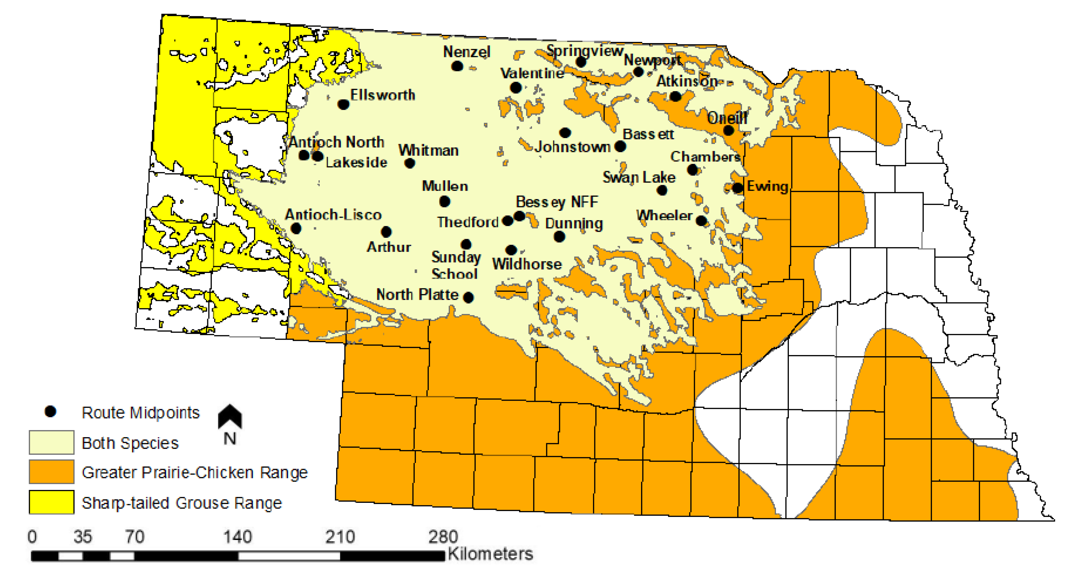
Figure 2.
State-wide cumulative annual hunter days in the field from 1955-2018, estimated from Nebraska’s annual small game hunter survey results. Blue trend line is LOESS spline with a grey 95% confidence interval. Data provided by NGPC.
Figure 2.
State-wide cumulative annual hunter days in the field from 1955-2018, estimated from Nebraska’s annual small game hunter survey results. Blue trend line is LOESS spline with a grey 95% confidence interval. Data provided by NGPC.
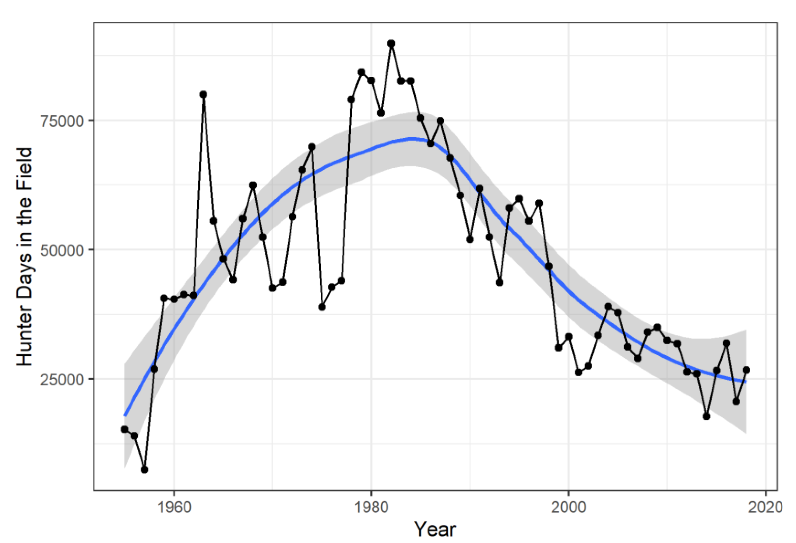
Figure 3.
Average number of birds of prey per Breeding Bird Survey (BBS) route from 1955-2018 in the Sandhills of Nebraska, USA. Data prior to the beginning of the BBS survey in 1967 reflects the first observed average count. Blue trend line is LOESS spline with a grey 95% confidence interval. Data taken from BBS (1966-2018).
Figure 3.
Average number of birds of prey per Breeding Bird Survey (BBS) route from 1955-2018 in the Sandhills of Nebraska, USA. Data prior to the beginning of the BBS survey in 1967 reflects the first observed average count. Blue trend line is LOESS spline with a grey 95% confidence interval. Data taken from BBS (1966-2018).
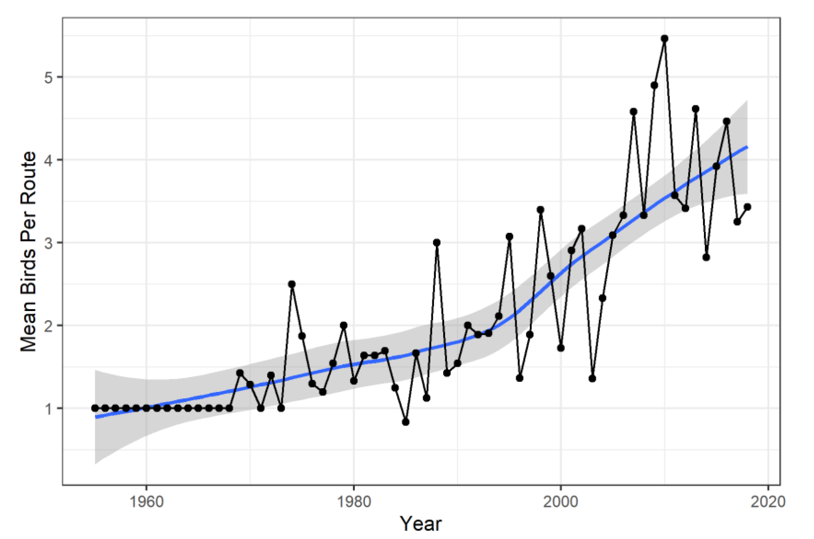
Figure 4.
Trends in cropland, hay and Conservation Reserve Program (CRP) area from 1955-2018 in the Sandhills of Nebraska, USA. Zero values at the start of the CRP time series reflect years prior to the start of the program. Note the scale of the CRP y-axis differs from the other panels to emphasize the trend. Blue trend lines are LOESS splines with grey 95% confidence intervals. Data from NASS (2026a) and USDA (2026).
Figure 4.
Trends in cropland, hay and Conservation Reserve Program (CRP) area from 1955-2018 in the Sandhills of Nebraska, USA. Zero values at the start of the CRP time series reflect years prior to the start of the program. Note the scale of the CRP y-axis differs from the other panels to emphasize the trend. Blue trend lines are LOESS splines with grey 95% confidence intervals. Data from NASS (2026a) and USDA (2026).
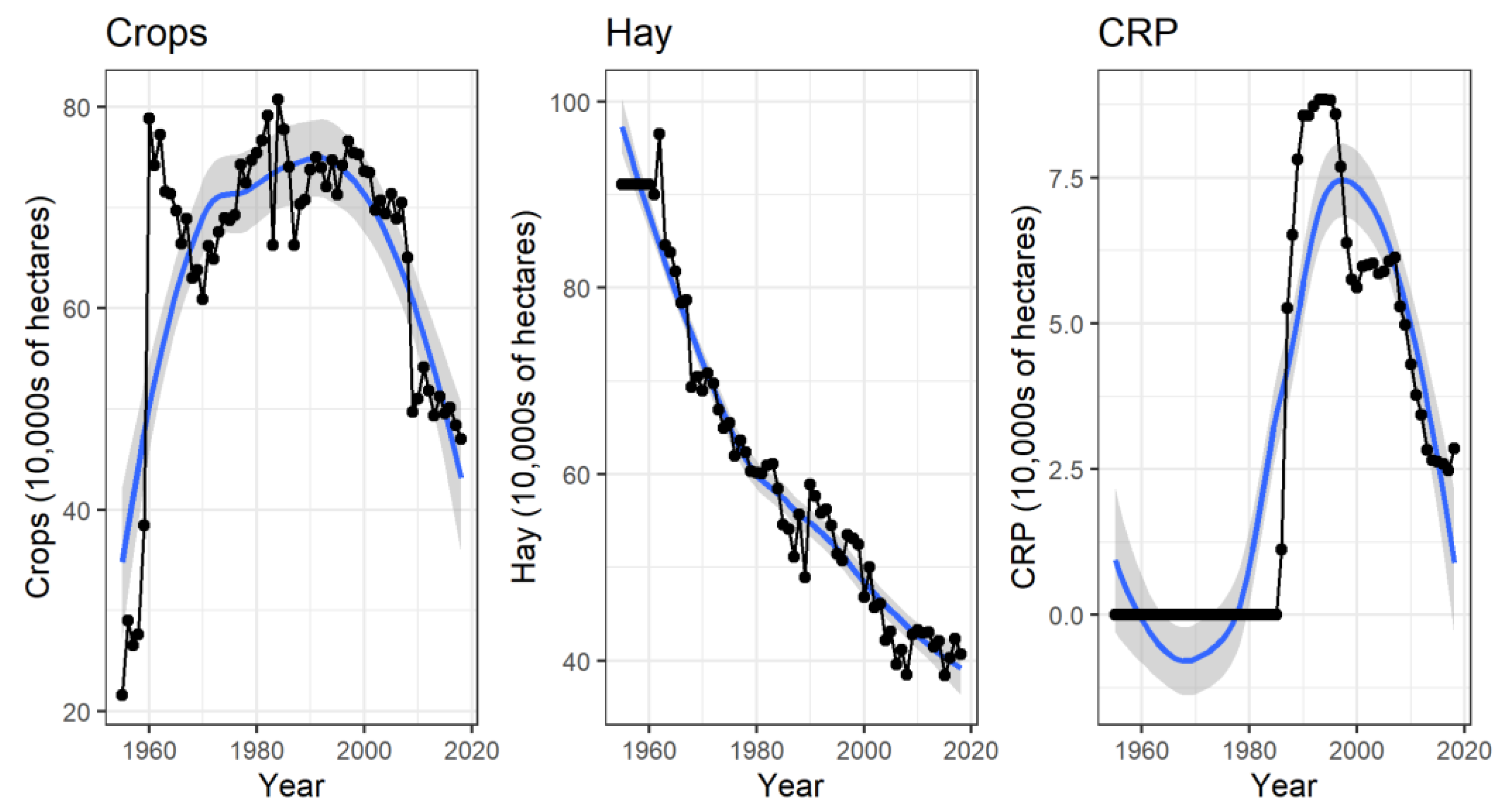
Figure 5.
Average grazing pressure in Animal Unit Months (AUMs) per hectare from 1955-2018 in the Sandhills of Nebraska, USA. The stair-step appearance of the trend line reflects the 5-year periodicity of the NASS (2026a) census data used to construct the index. Blue trend line is LOESS spline with a grey 95% confidence interval.
Figure 5.
Average grazing pressure in Animal Unit Months (AUMs) per hectare from 1955-2018 in the Sandhills of Nebraska, USA. The stair-step appearance of the trend line reflects the 5-year periodicity of the NASS (2026a) census data used to construct the index. Blue trend line is LOESS spline with a grey 95% confidence interval.
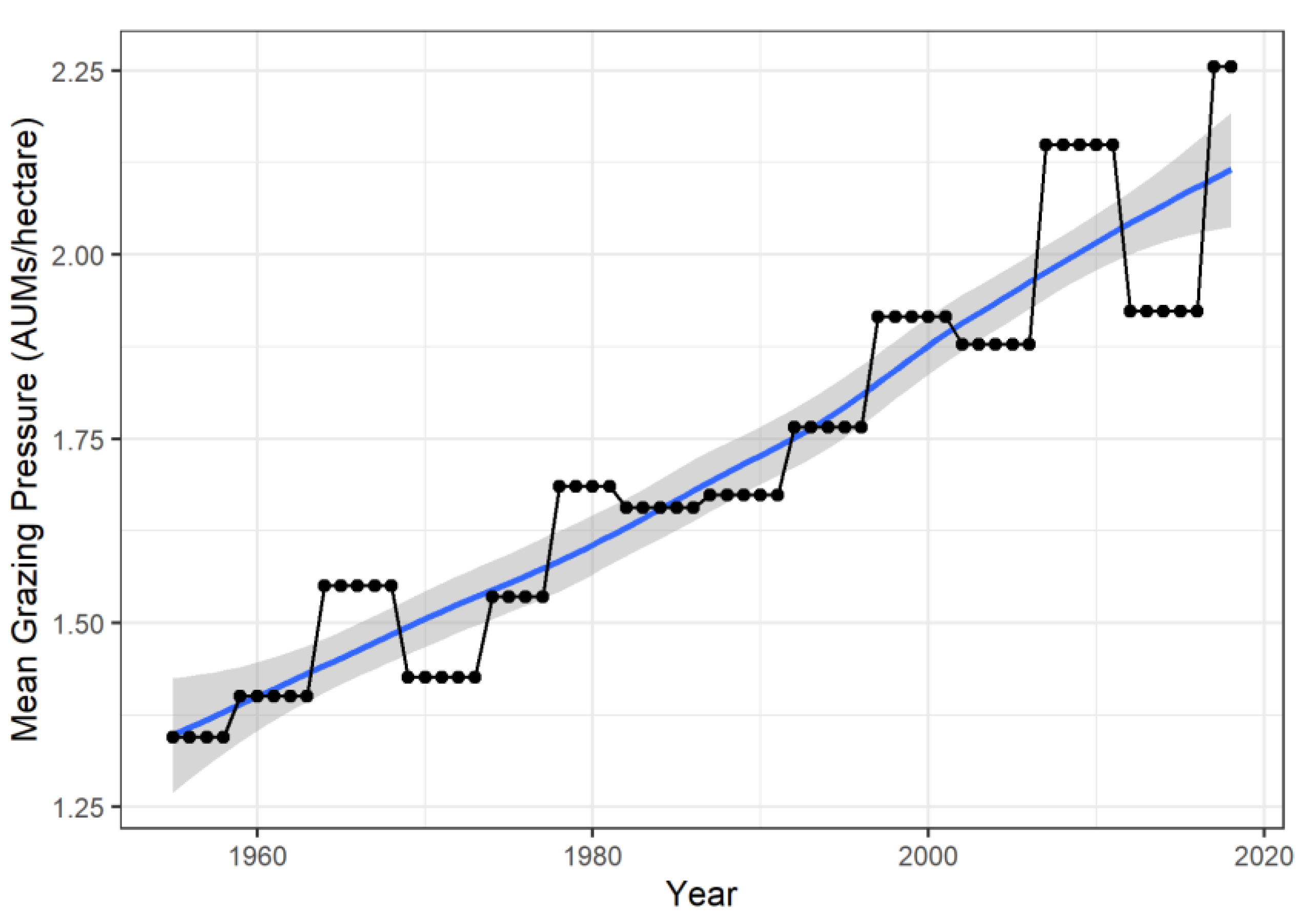
Figure 6.
Self-Calibrating Palmer Drought Severity Index (SCPDSI) and Accumulated Winter Season Severity Index (AWSSI) values from 1955-2018 for the Sandhills of Nebraska, USA. Blue trend lines are LOESS splines with grey 95% confidence intervals. Data from NDMC (2026) and ACIS (2026).
Figure 6.
Self-Calibrating Palmer Drought Severity Index (SCPDSI) and Accumulated Winter Season Severity Index (AWSSI) values from 1955-2018 for the Sandhills of Nebraska, USA. Blue trend lines are LOESS splines with grey 95% confidence intervals. Data from NDMC (2026) and ACIS (2026).
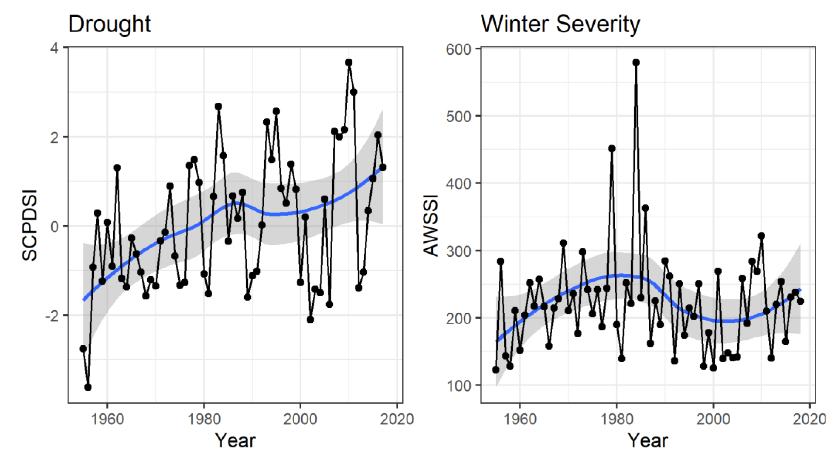

Table 1.
Sources of long-term environmental monitoring data predating the advent of remote sensing technologies in the 1970s through present day, with an emphasis on spatial coverage of the continental United States of America (US). See citations for data access URLs.
Table 1.
Sources of long-term environmental monitoring data predating the advent of remote sensing technologies in the 1970s through present day, with an emphasis on spatial coverage of the continental United States of America (US). See citations for data access URLs.
| Dataset | Agency | Variable | Earliest Record |
Temporal Resolution |
Spatial Resolution |
Geographic Extent |
|---|---|---|---|---|---|---|
| COOP/GHCN [82] | NOAA | Temp/Precip/Snow | 1800s | Daily | Station | U.S. |
| nClimDiv/nClimGrid [83] | NOAA | Temp/Precip | 1895 | Monthly | 5x5 Degree Lat/Long | U.S. |
| NWIS [84] | USGS | Streamflow | 1800s | Daily/Subdaily | Gauge | U.S. |
| Stream Temperature [85] | USGS | Mean/Min/Max Temp. | 1894 | Daily/Subdaily | Stream Segment | U.S. |
| Groundwater [86] | USGS | Water Table | Early 1900s | Monthly/Irregular | Well | U.S. |
| STORET [87] | EPA | Water Quality | 1965 | Daily/Irregular | Site | U.S. |
| Snow Course [88] | NRCS | SWE/Snow Depth | 1906 | Seasonal | Course | Western U.S. |
| NASN [89] | EPA | TSP/Trace Pollutants | 1957 | Biweekly | Monitor | U.S. |
| AQS [89] | EPA | Air Pollutants | 1950s/60s | Variable | Monitor | U.S. |
| Water quality [84] | USGS/EPA | Chemistry/Sediment | Early 1900s | Irregular | Site | U.S. |
| Geoecology [90] | ORNL/ NASA |
Multiple | 1941 | Variable | County | CONUS |
| Paleo archives [91] | NOAA | Tree Rings/Sediments | Centuries–Millennia | Variable | Site | U.S./Global |
| SPI [92] | NOAA | Drought | 1895 | 9-Month | Station | U.S. |
| LBDA [93] | NOAA | Historic Drought | 0 CE | Annual | 1/2 Degree Lat/Long | U.S. |
| Wildfire [94] | USGS | Historic Wildfire | 1878 | Annual | Burn Polygon | U.S. |
| NASS [95] | USDA | Cropland/Livestock | ~1900 | Annual | County | U.S. |
| Aerial Photography [96] | National Archives | Land Use Change | 1918-2011 | Various | Various | U.S. |
| First Development [97] | USGS | Urban Development | 1940 | 10-year | 100m | U.S. |
| Breeding Bird (BBS) [98] | USGS | Bird Population Index | 1966 | Annual | Route | U.S. |
| Christmas Bird (CBC) [99] | Audubon | Bird Occupancy | 1900 | Annual | Point | U.S. |
| GRSF [100] | United Nations | Fish Population Index | ~1950 | Annual/Irregular | Fishery | Global |
Table 2.
Cattle weights, change in cattle weights over time, Animal Unit Month (AUM) equivalents, and months on pasture by cattle type for grazing regions in Nebraska used as inputs in the grazing index calculation. Modified from Cumming et al. 2019.
Table 2.
Cattle weights, change in cattle weights over time, Animal Unit Month (AUM) equivalents, and months on pasture by cattle type for grazing regions in Nebraska used as inputs in the grazing index calculation. Modified from Cumming et al. 2019.
| Metric | Calving Season | Cow Calf Pairs | Non-Lactating Cows | Replacement Heifer Yearlings | Bulls | Stockers |
|---|---|---|---|---|---|---|
| Average Weight for the Grazing Period (2007) | 590 kg cow and 300 kg calf | 590 kg | 408 kg | 907 kg | 318 kg | |
| Total Change in Weight (kgs) 1975-2005 | 136 kg cows, 14 kg per calf for each 45 kg cow weight gain | 136 kg | 159 kg | 159 kg | 136 kg | |
| Animal Units (2007) | 1.6 | 1.3 | 0.9 | 2.0 | 0.7 | |
| Sandhills (Months on Pasture) | Spring | 5 | 4.5 | 9.5 | 9.5 | 4 |
| Panhandle (Months on Pasture) | Spring | 5.5 | 1 | 5.5 | 6.5 | 4 |
| South Central (Months on Pasture) | Spring | 5 | 0 | 5 | 2 | 2 |
| North Central (Months on Pasture) | Spring (90%) | 5.5 | 0 | 5.5 | 3 | 3 |
| Fall (10%) | 2 | 3.5 |
Disclaimer/Publisher’s Note: The statements, opinions and data contained in all publications are solely those of the individual author(s) and contributor(s) and not of MDPI and/or the editor(s). MDPI and/or the editor(s) disclaim responsibility for any injury to people or property resulting from any ideas, methods, instructions or products referred to in the content. |
© 2026 by the authors. Licensee MDPI, Basel, Switzerland. This article is an open access article distributed under the terms and conditions of the Creative Commons Attribution (CC BY) license (http://creativecommons.org/licenses/by/4.0/).
Copyright: This open access article is published under a Creative Commons CC BY 4.0 license, which permit the free download, distribution, and reuse, provided that the author and preprint are cited in any reuse.