

Submitted:
10 November 2026
Posted:
12 November 2026
You are already at the latest version
Abstract
Japan's official non-destructive radiocaesium screening method allows food-specific screening levels (SL) to be set by linear regression against reference germanium (Ge) spectrometry. It does not cover wild game meat, in which concentrations above the 100 Bq kg−1 standard limit are still found in Fukushima Prefecture. We evaluated this regression-based approach with intact quadriceps femoris muscle blocks from 126 wild animals (wild boar, Asian black bear, and sika deer), measured unfrozen and/or frozen with commercial CsI(Tl) and NaI(Tl) instruments. SL point estimates ranged from 43.2 to 81.1 Bq kg−1 in all eight strata, meeting the requirement of SL ≥ 25 Bq kg−1, although one lower bootstrap confidence limit was 25.4 Bq kg−1. No sample exceeding the standard limit was screened negative in the primary or leave-one-out evaluation. The upper 95% confidence limits of the false-negative rate were 6.7% (frozen) and 10.0% (unfrozen) for wild boar. For bear and deer, with only 4 and 5 exceeding samples, they were 60.2% and 52.2%. Residual variance increased with concentration in most strata and was dominated by sample-specific deviations rather than replicate variation. Under a fitted variance-function model, the model-based miss probability at 100 Bq kg−1 was 0.10%–0.43% for wild boar, but was higher (1.26%–4.60%) and model-dependent for bear and deer. Paired measurements showed that frozen wild boar blocks gave lower indications than unfrozen blocks. Although the SL requirement was met, the implied false-negative control depended on the concentration-dependent error structure and the calibration data.
Keywords:
radiocaesium
; wild game meat
; non-destructive screening
; screening level
; heteroscedasticity
; Fukushima
1. Introduction
Following the Fukushima Daiichi Nuclear Power Plant accident in 2011, Japan's Ministry of Health, Labour and Welfare (MHLW) set a standard limit of 100 Bq kg−1 for radiocaesium (134Cs and 137Cs) in general foods in April 2012 (MHLW, 2012c). Over the subsequent decade, exceedances of this standard limit have become largely restricted to forest products and wildlife that cannot be readily managed through agricultural interventions (Nakamura et al., 2022). Free-ranging game animals belong to this group. Long-term monitoring of wild boar (Sus scrofa) across Fukushima Prefecture showed declining muscle 137Cs concentrations, with region-specific ecological half-lives of 3.0–9.2 years (Komatsu and Ikushima, 2026). Concentrations also vary with season and capture area (Nemoto et al., 2018; Cui et al., 2020; Saito et al., 2022). Persistent radiocaesium contamination of wild boar has been reported in Europe after the Chernobyl accident (Steinhauser and Saey, 2016; Stäger et al., 2023). Radiocaesium contamination has similarly been documented in Asian black bear (Ursus thibetanus) (Nemoto et al., 2018) and sika deer (Cervus nippon) (Koganezawa et al., 2019; Hayashi et al., 2016). Under national guidelines issued by the Nuclear Emergency Response Headquarters (NERHQ), meat from these game species remains among the items with concentrations above the standard limit, including in Fukushima Prefecture. Distribution restrictions can be partially lifted only under a prefectural shipping and inspection policy (NERHQ, 2024).
The official reference method for food radiocaesium testing relies on high-purity germanium (Ge) semiconductor gamma-ray spectrometry, which requires chopping, homogenizing, and packing samples into calibrated geometry containers (MHLW, 2012b). Official screening methods using scintillation spectrometers also require prepared samples in containers (MHLW, 2012a; Yamada et al., 2017). Because destructive preparation makes the food unsaleable, container-based methods are suited to sampling surveys rather than to the testing of every item before shipment (Yamada et al., 2023). For pre-shipment testing, non-destructive instruments that measure whole foods inside plastic bags were developed after the accident (Ishii, 2015, 2018) and are now used at municipal monitoring stations and producer facilities in Fukushima Prefecture (Yamada et al., 2019). Because these instruments measure intact items without a standardized container geometry, detector response is influenced by sample mass, thickness, shape, and the spatial distribution of radiocaesium within the item (Yamada et al., 2023).
To enable the use of these instruments in inspection, the MHLW introduced an official non-destructive screening method in 2021 (MHLW, 2024, 2025). Under this method, an instrument- and food-specific screening level (SL) must be set so that the 99% upper limit of indications at the SL lies below the indication obtained at the standard limit. This upper limit can be obtained from repeated measurements at the SL or from the one-sided 99% upper prediction bound of a linear regression of instrument indications on Ge results. The worked examples of the method use this regression-based approach (MHLW, 2025). To qualify for screening, the derived SL must be at least 25 Bq kg−1. A food whose indication is above the corresponding device threshold (, the device indication corresponding to the SL) cannot be judged to be below the standard limit and must be confirmed by Ge spectrometry. A food with an indication at or below this threshold is reported as being below the screening level (MHLW, 2025). A regression approach of this kind was evaluated across multiple non-destructive instruments for wild mushrooms and bamboo shoots (Yamada et al., 2023). Currently, however, the official scope of the method is limited to seven kinds of mushrooms, bamboo shoots with sheaths, and the wild vegetable koshiabura; wild game meat is not included (MHLW, 2025).
Intact game meat differs physically from bagged plant foods. A game thigh is a large, dense muscle block whose mass, thickness, and shape vary substantially between animals, and blocks may be measured in either an unfrozen or a frozen state. Non-destructive radiocaesium monitoring of meat-producing animals has an established history dating to the Chernobyl accident, when portable NaI detectors calibrated against muscle samples were used to screen live sheep, cattle, reindeer, and dressed carcasses (Brynildsen and Strand, 1994). In live sheep, an operational rejection threshold was similarly derived from regression against muscle Ge spectrometry (Meredith et al., 1988). Field measurements of whole or field-dressed deer and feral pigs have been investigated more recently (Whiteside et al., 2020). In Japan, an MHLW-funded research report described exploratory non-destructive measurements of a small number of wild boar samples, but the data were insufficient to characterize regression relationships with Ge results (Hachisuka, 2018). To our knowledge, the regression-based approach of the MHLW method has not been systematically evaluated for intact game meat in a peer-reviewed study.
The regression-based approach also assumes homoscedasticity, estimating a single residual variance over the whole calibration range. Under constant variance, deriving an SL from a one-sided 99% prediction interval corresponds to a nominal probability of approximately 1% that a sample exactly at the 100 Bq kg−1 standard limit gives an indication below the device threshold. This correspondence follows the classical formulation of calibration prediction limits as decision error probabilities (Hubaux and Vos, 1970). This nominal ~1% value represents a statistical interpretation adopted in the present study rather than an explicit regulatory specification. In analytical instrumentation, however, measurement errors often increase with analyte concentration (Zorn et al., 1997). When heteroscedasticity is present, the implied miss probability at the standard limit depends on the concentration distribution of the calibration samples, a relationship that we did not find quantified for non-destructive food screening.
In this study, we applied the regression-based approach of the MHLW method to intact quadriceps femoris muscle blocks from wild boar, Asian black bear, and sika deer collected in Fukushima Prefecture. Samples were measured in unfrozen and/or frozen states with two commercial scintillation instruments (one CsI(Tl) and one NaI(Tl)) and then analysed by Ge semiconductor spectrometry. Our specific objectives were: (i) to estimate instrument-, species-, and sample-state-specific screening levels and device thresholds () along with their bootstrap confidence intervals; (ii) to evaluate classification performance against the 100 Bq kg−1 standard limit using internal leave-one-out cross-validation and temporal validation; and (iii) to characterize the measurement-error structure and assess its implications for false-negative control under heteroscedasticity. Because wild game meat is not a target food of the current MHLW method, this work represents an empirical performance evaluation rather than a regulatory endorsement.
2. Materials and methods
2.1. Study Samples And Preparation
Intact quadriceps femoris muscle blocks were collected from 126 wild animals in Fukushima Prefecture, Japan, between June 2023 and November 2024, comprising 74 wild boar, 24 Asian black bears, and 28 sika deer. The animals were captured for nuisance wildlife control or by hunting in four municipalities (Supplementary Methods S1). Of these, 73 were captured in Japanese fiscal year (FY; April–March) 2023 and 53 in FY2024. Some of these measurements were previously reported in a conference abstract and a government research report (Maekawa et al., 2024; Yamada, 2025). S-Table 1 compares these reports with the present study.
Ethical approval was not required for this study because no live animals were experimented upon; all muscle samples were obtained from wild animals legally culled for nuisance wildlife control or harvested by licensed hunting. To prepare each sample, outer tissues were trimmed to remove surface hair, soil, and other material. The block was then sealed inside a resealable plastic bag without shaping or homogenization. Bagged blocks were measured non-destructively (Section 2.2) in an unfrozen state, a frozen state, or both. After all non-destructive measurements, a subsample (78.3–142.2 g wet mass) was cut from each block for reference Ge spectrometry. The subsample was thawed, minced, freeze-dried, and ground with a mixer before being packed into a cylindrical U-8 geometry container (Section 2.3). Whole block masses ranged from 171 to 2,860 g (Table 1). Capture dates and Ge counting schedules stratified by species and sample state are detailed in S-Table 2.
Two sample states were defined operationally. Unfrozen measurements were made on blocks before freezing, 1–6 days after capture. Frozen measurements were made on frozen blocks without thawing, 2–115 days after capture. Of the 126 blocks, 56 were measured in both states (the same block measured unfrozen and then frozen, with 1–13 days between the two measurements), 69 were received frozen and measured only in the frozen state, and 1 block (sika deer) was measured only in the unfrozen state.

Table 1.
Sample characteristics and analysis sets by species and sample state.
| Species | State | Role | Individuals (n) | FY2023 / FY2024 (n) | Block weight, g: median (range); missing | Ge-derived 134Cs + 137Cs (Bq kg−1 wet mass): median (range) | Ge > 100 (n) | Ge 50–250 (n) | Ge > 250 (n) | Days from capture to device measurement: median (range) | Evaluation set, A / B (n) | Calibration set, A / B (n) |
| Wild boar | Frozen | Main stratum | 74 | 40 / 34 | 845 (171–1510); missing 3 | 175.5 (8.9–11101.0) | 53 | 33 | 27 | 8 (2–115) | 74 / 74 | 47 / 47 |
| Wild boar | Unfrozen | Main stratum | 50 | 25 / 25 | 774 (171–1374); missing 0 | 157.6 (15.3–1847.0) | 35 | 22 | 18 | 2 (1–6) | 50 / 50 | 32 / 31 |
| Asian black bear | Frozen | Main stratum | 24 | 16 / 8 | 1202 (509–2860); missing 4 | 32.4 (0.0–242.6) | 4 | 9 | 0 | 9 (2–65) | 24 / 24 | 23 / 23 |
| Asian black bear | Unfrozen | Descriptive only | 5 | 4 / 1 | 1021 (546–2859); missing 0 | 30.1 (26.3–45.0) | 0 | 0 | 0 | 4 (1–4) | 5 / 5 | 5 / 5 |
| Sika deer | Frozen | Main stratum | 27 | 16 / 11 | 1004 (197–2006); missing 0 | 25.3 (2.4–340.6) | 5 | 7 | 1 | 9 (2–79) | 27 / 27 | 26 / 24 |
| Sika deer | Unfrozen | Descriptive only | 2 | 1 / 1 | 866 (729–1004); missing 0 | 17.6 (5.8–29.3) | 0 | 0 | 0 | 1.5 (1–2) | 2 / 2 | 2 / 2 |
One thigh block per individual. Unfrozen and frozen wild boar measurements refer to the same blocks measured before and after freezing. Block weights, Ge-derived concentrations and days are summarized over the device A rows.Ge-derived 134Cs + 137Cs (Bq kg−1 wet mass): Ge-measured 137Cs plus detected 134Cs, each decay-corrected from the capture date to the device measurement date; Ge 137Cs not detected = 0. Evaluation set: all rows with Ge and device readings, without a Ge range limit. Calibration set: at least one detected replicate and 0 < Ge ≤ 250 Bq kg−1 wet mass. Unfrozen Asian black bear and unfrozen sika deer are descriptive only (not main strata). Measurement conditions: device A frozen-block measurements were made outside the condition stated in the manufacturer's instruction manual, and some device B blocks were outside the manufacturer-stated weight range (300–2,000 g); all rows were retained (S-Table 3). Devices: A: Legumes Light (FD-08Cs1000-1), CsI(Tl); B: AFT-NDA2, NaI(Tl).
2.2. Non-Destructive Measurement
Non-destructive measurements were made with two commercial radiocaesium instruments at the Fukushima Prefectural Centre for Environmental Creation. The Legumes Light (model FD-08Cs1000-1; Techno-X Co., Ltd., Japan) has a CsI(Tl) scintillation detector (φ11 × 2.5 cm) and 50 mm lead shielding. The AFT-NDA2 (Advanced Fusion Technology Co., Ltd., Japan; Japanese product name そのままはかるNDA2) has a NaI(Tl) scintillation detector (φ12.7 × 12.7 cm) and 35–50 mm lead shielding. In all tables and figures, these instruments are labelled A (Legumes Light, CsI(Tl)) and B (AFT-NDA2, NaI(Tl)).
Each bagged block was measured with both instruments on the same day in a given sample state. For each instrument–state combination, the standard protocol was four consecutive 600-s readings: two readings on the initial resting face followed by two readings after turning the block over, typically in that order. No specific anatomical or geometric criteria defined the two faces. For three unfrozen Asian black bear blocks in a descriptive stratum (6 records), only one 600-s reading per face was available (Supplementary Methods S1). The MHLW method recommends re-mixing or re-dispersing loose food items between readings to reduce the effect of uneven radiocaesium distribution (MHLW, 2025). An intact meat block cannot be re-dispersed, so turning the block over was the only planned repositioning. Operational settings conformed to manufacturer documentation (Supplementary Methods S2). For the Legumes Light, the counting geometry setting ("container equivalent") best approximating block dimensions was selected. For the AFT-NDA2, operator inputs included the species-specific sample designation, sample form specified as "packed in a bag", container type set to "bag only", and block mass. The instrument internally derives counting efficiency from the entered mass and a density preset for the sample designation, by a calculation not disclosed by the manufacturer. Both instruments received annual maintenance and calibration under contract with Fukushima Prefecture. Daily pre-operational quality-control records for the Legumes Light (background blank and 40K check sample) are archived from February 2024 onward, coinciding with the export period of its digital result logs.
Two measurement conditions were outside the manufacturers' specifications. First, the instruction manual for the Legumes Light specifies that frozen specimens cannot be measured; frozen-state measurements on this instrument thus represent an application outside the manufacturer's stated specimen condition. Second, technical documentation for the AFT-NDA2 specifies an operational sample mass range of 300–2,000 g. Among the AFT-NDA2 measurement records, 3 weighed below 300 g, 4 were above 2,000 g, and 7 lacked mass entries in the measurement workbook. No samples were excluded based on these deviations; all affected records are flagged in S-Table 3.
2.3. Germanium Semiconductor Spectrometry
Reference gamma-ray spectrometry was performed at the Fukushima Prefectural Centre for Environmental Creation using a high-purity germanium detector system (Canberra GA-CHGR), which was calibrated annually by a contracted service provider. Prepared samples packed in U-8 containers (Section 2.1) were counted for 3,600 s (73 wild boar) or 10,000 s (24 Asian black bears, 28 sika deer, and 1 wild boar) (S-Table 2).
Activity concentrations of 134Cs and 137Cs were determined on a dry-mass basis, converted to wet tissue concentrations using sample-specific dry-to-wet mass ratios (0.168–0.295), and decay-corrected to the animal capture date by the testing laboratory. Values below the detection limit were recorded as not detected; 134Cs was detected in 21 and 137Cs in 125 of the 126 individuals. All activity concentrations in this article are reported in Bq kg−1 wet mass.
For calibration and performance evaluation, activity concentrations were decay-corrected from the capture date to the date of each non-destructive measurement using half-lives of 2.0652 y for 134Cs and 30.08 y for 137Cs (Supplementary Methods S3). The reference radiocaesium concentration, , was defined as the decay-corrected 137Cs concentration plus the decay-corrected 134Cs concentration when 134Cs was detected. When a nuclide was not detected, its contribution was set to zero without adding the detection limit, following the official MHLW test method and its accompanying guidance (MHLW, 2012b, 2015). Accordingly, the single animal with undetected 137Cs was assigned . Because the unfrozen and frozen measurements were made on different dates, was calculated separately for each measurement.
Table 2.
Calibration and screening levels obtained with the regression-based approach in the eight main strata.
Table 2.
Calibration and screening levels obtained with the regression-based approach in the eight main strata.
| Device | Species | State | n (calibration) | Slope (SE) | Intercept (SE), Bq kg−1 | s, Bq kg−1 | SL [95% CI], Bq kg−1 wet mass | T_SL [95% CI], Bq kg−1 | SL, S-ND1 complete-case (n) |
| A: Legumes Light, CsI(Tl) | Wild boar | Frozen | 47 | 1.137 (0.057) | 2.86 (7.43) | 26.21 | 43.2 [25.4, 63.6] | 51.9 [32.5, 75.7] | 42.3 (46) |
| A: Legumes Light, CsI(Tl) | Wild boar | Unfrozen | 32 | 1.366 (0.076) | -0.09 (9.27) | 26.29 | 51.4 [35.3, 71.5] | 70.1 [48.3, 98.2] | 51.4 (32) |
| A: Legumes Light, CsI(Tl) | Asian black bear | Frozen | 23 | 0.881 (0.040) | 6.11 (3.40) | 11.72 | 65.8 [54.1, 86.1] | 64.1 [54.9, 93.1] | 64.8 (22) |
| A: Legumes Light, CsI(Tl) | Sika deer | Frozen | 26 | 0.953 (0.044) | 6.56 (3.49) | 13.94 | 62.8 [47.6, 88.9] | 66.5 [51.8, 100.7] | 57.3 (21) |
| B: AFT-NDA2, NaI(Tl) | Wild boar | Frozen | 47 | 0.808 (0.027) | 3.57 (3.56) | 12.56 | 61.9 [51.7, 74.0] | 53.6 [46.5, 62.9] | 60.8 (45) |
| B: AFT-NDA2, NaI(Tl) | Wild boar | Unfrozen | 31 | 0.996 (0.038) | -1.59 (4.69) | 12.64 | 68.0 [57.8, 81.7] | 66.2 [55.8, 79.9] | 68.0 (31) |
| B: AFT-NDA2, NaI(Tl) | Asian black bear | Frozen | 23 | 0.683 (0.017) | 4.56 (1.45) | 4.99 | 81.1 [75.0, 88.5] | 59.9 [54.2, 67.1] | 80.3 (20) |
| B: AFT-NDA2, NaI(Tl) | Sika deer | Frozen | 24 | 0.738 (0.022) | 4.24 (1.84) | 6.91 | 76.0 [68.2, 88.9] | 60.4 [55.2, 73.2] | 72.3 (18) |
Regression-based approach evaluated here: ordinary least squares of the device indication (arithmetic mean of the detected replicates among the four standard 600-s readings, two on each face of the block) on the Ge-derived concentration within the calibration set (0 < Ge ≤ 250 Bq kg−1 wet mass). SL (screening level) is the Ge-derived concentration at which the one-sided 99% upper prediction bound equals ŷ_100, the fitted indication at 100 Bq kg−1 wet mass; T_SL = intercept + slope × SL is the corresponding device threshold (the device indication corresponding to the screening level in the official screening notice). In this article, SL denotes only the screening level on the Ge-derived concentration scale. s: residual standard deviation. 95% CIs: individual-level bootstrap percentile intervals (B = 2,000; seed 20261002 + stratum number); no resample lacked a solution. Bootstrap end points are subject to Monte Carlo variation: for device A, wild boar, Frozen, the lower bound (25.4 Bq kg−1 wet mass) is close to the 25 Bq kg−1 wet mass requirement and may cross it under Monte Carlo variation (prespecified seed and B retained). S-ND1: complete-case rule (only samples with all four replicates detected), prespecified to be reported alongside the primary rule. Full calibration statistics, including the pooled and descriptive-only strata, are in S-Table 4. Devices: A: Legumes Light (FD-08Cs1000-1), CsI(Tl); B: AFT-NDA2, NaI(Tl).
2.4. Analysis Populations and Variables
One quadriceps femoris muscle block was obtained from each animal. Each block was measured in an unfrozen state, a frozen state, or both, using two instruments. The dataset comprised 364 animal–state–instrument records. Analysis strata were defined by crossing instrument, species, and sample state. The main analysis included eight strata: frozen samples of all three species and unfrozen wild boar samples, each measured with two instruments. Unfrozen Asian black bear (n = 5) and sika deer (n = 2) samples were evaluated descriptively because of their small sample sizes.
For each record, the device indication, , was calculated as the arithmetic mean of the detected readings among the four replicate readings (two for the records noted in Section 2.2). This follows MHLW worked examples that average the available readings while excluding non-detects (MHLW, 2025). For the Legumes Light, a reading (total 134Cs + 137Cs concentration) was treated as detected when a numeric value was reported. For the AFT-NDA2, a reading was considered detected if a numeric total was reported, or if the total was displayed as "<25.0" (indicating a concentration below the instrument's lower measurement limit) but accompanied by a numeric 137Cs value. In the latter case, the 137Cs value was used (Supplementary Methods S2). Numeric totals below 25 Bq kg−1 recorded in the laboratory's measurement workbook without the instrument output were treated in the same way. Records in which all replicate readings were non-detects (all-ND records) received no numeric indication: they were excluded from calibration regressions and classified as screen-negative. Test runs, interrupted measurements, and non-standard counting times were excluded, and duplicate workbook transcriptions were consolidated. For the one block with an explicit repeat session under the standard protocol, the last complete set of readings was used (Supplementary Methods S1; S-REP1).
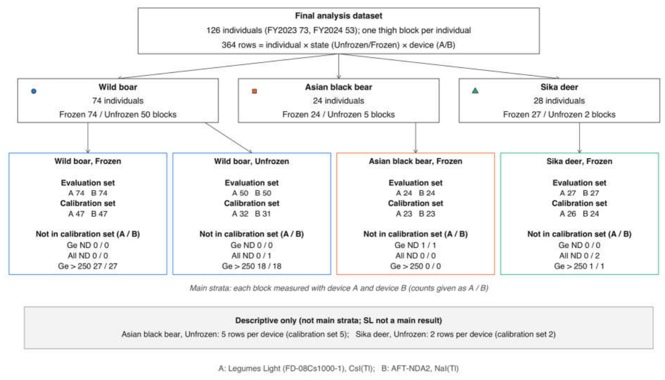
Two analysis sets were defined within each stratum. The calibration set included all records with at least one detected reading and a reference concentration within Bq kg−1. The evaluation set included all records with both a Ge result and device readings, without restriction on concentration. A sample was regarded as truly exceeding the standard limit when Bq kg−1 on the date of the non-destructive measurement. The flow of samples into these sets is shown in Figure 1.
Instrument readings, Ge results, and sample logs were compiled into a single dataset linked to the source files (Supplementary Methods S1). The dataset, population definitions, data-handling rules, and statistical procedures (Section 2.4, Section 2.5, Section 2.6, Section 2.7 and Section 2.8) were fixed before the primary analysis was run; any analysis introduced later is identified as post hoc.
Figure 1.
Study population and analysis sets. One thigh block per individual; blocks were measured unfrozen and/or frozen, each with both devices. Evaluation set: all rows with Ge and device readings, without a Ge range limit; rows with all replicates not detected (All ND) are screen-negative for classification only. Calibration set: at least one detected replicate and 0 < Ge ≤ 250 Bq kg−1 wet mass. Rows outside the calibration set are counted once, in the priority order Ge 137Cs not detected (Ge ND) > All ND > Ge > 250 Bq kg−1 wet mass (W23-119 is both Ge ND and All ND and is counted as Ge ND); this is a display convention and does not change set membership. Unfrozen Asian black bear and unfrozen sika deer are descriptive only. Devices: A: Legumes Light (FD-08Cs1000-1), CsI(Tl); B: AFT-NDA2, NaI(Tl).
Figure 1.
Study population and analysis sets. One thigh block per individual; blocks were measured unfrozen and/or frozen, each with both devices. Evaluation set: all rows with Ge and device readings, without a Ge range limit; rows with all replicates not detected (All ND) are screen-negative for classification only. Calibration set: at least one detected replicate and 0 < Ge ≤ 250 Bq kg−1 wet mass. Rows outside the calibration set are counted once, in the priority order Ge 137Cs not detected (Ge ND) > All ND > Ge > 250 Bq kg−1 wet mass (W23-119 is both Ge ND and All ND and is counted as Ge ND); this is a display convention and does not change set membership. Unfrozen Asian black bear and unfrozen sika deer are descriptive only. Devices: A: Legumes Light (FD-08Cs1000-1), CsI(Tl); B: AFT-NDA2, NaI(Tl).
2.5. Screening-Level Analysis According to the MHLW Method
Screening levels were derived separately for each stratum using the regression-based approach of the MHLW non-destructive screening method in its current version (MHLW, 2025). The non-destructive measurements (September 2023 to November 2024) were made while the 2023 and 2024 versions of the method were in force (MHLW, 2023, 2024). The statistical requirements used here (the 99% criterion, its regression-based approach and the requirement SL ≥ 25 Bq kg−1) are the same in all three versions. Within each calibration set, the device indication was regressed on the reference concentration by ordinary least squares (OLS) to estimate the slope , intercept , and residual standard deviation . The predicted device indication at the 100 Bq kg−1 standard limit was calculated as , and the one-sided 99% upper prediction bound of the device indication was:
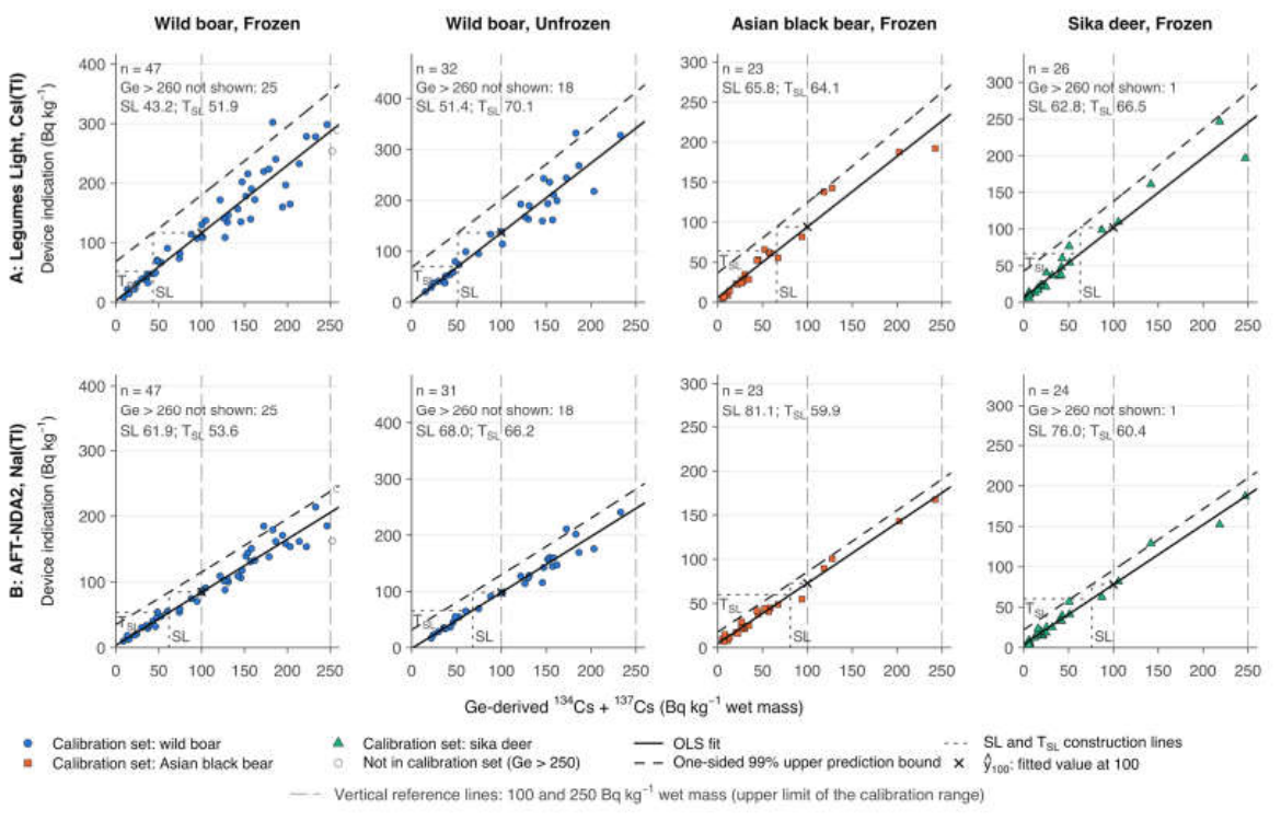
where and denote the sample mean and corrected sum of squares of in the calibration set. The screening level (SL) is defined as the reference concentration whose upper prediction bound equals the predicted indication at the standard limit, . This root was determined numerically using R's uniroot function (search interval −1000 to 100 Bq kg−1; convergence tolerance 10−8). The corresponding device threshold on the scale of the instrument display was calculated as . The worked examples of the MHLW method call this quantity the device indication corresponding to the screening level. Because those examples also attach the label SL to this device-scale value, we use SL only for the screening level on the reference-concentration scale. Under the MHLW method, the screening level must be at least 25 Bq kg−1 (MHLW, 2025). The geometric construction of SL and is illustrated in Figure 2.
Statistical uncertainty in SL and was estimated with a non-parametric bootstrap at the animal level. Animals in each stratum's calibration set were sampled with replacement in B = 2,000 resamples (random seed 20261002 + stratum number), and SL and were re-estimated in each resample to obtain 95% percentile confidence intervals (Supplementary Methods S4). Resamples without a valid root were counted. Calibration scatterplots for all strata are presented in S-Figure 1, and complete regression diagnostics across all strata, including exploratory pooled sets, are compiled in S-Table 4.
Figure 2.
Calibration with the regression-based approach in the eight main strata. Rows: devices; columns: species and sample state. Device indication: arithmetic mean of the detected replicates among the four standard 600-s readings (two on each face of the block). Ge-derived 134Cs + 137Cs: Ge-measured 137Cs plus detected 134Cs, each decay-corrected from the capture date to the device measurement date (Bq kg−1 wet mass). Filled symbols: calibration set; open grey symbols: samples outside the calibration set with Ge ≤ 260 Bq kg−1 wet mass (samples above 260 are not shown; their number is given in each panel). Solid line: ordinary least-squares fit; dashed line: one-sided 99% upper prediction bound; dotted lines: construction of the screening level SL (vertical) and the device threshold T_SL (horizontal); at SL the upper prediction bound equals ŷ_100, the fitted value at 100 Bq kg−1 wet mass (cross). SL and T_SL values are given in each panel. Grey long-dashed lines: 100 and 250 Bq kg−1 wet mass (upper limit of the calibration range). Symbols and colours denote species throughout. Devices: A: Legumes Light (FD-08Cs1000-1), CsI(Tl); B: AFT-NDA2, NaI(Tl).
Figure 2.
Calibration with the regression-based approach in the eight main strata. Rows: devices; columns: species and sample state. Device indication: arithmetic mean of the detected replicates among the four standard 600-s readings (two on each face of the block). Ge-derived 134Cs + 137Cs: Ge-measured 137Cs plus detected 134Cs, each decay-corrected from the capture date to the device measurement date (Bq kg−1 wet mass). Filled symbols: calibration set; open grey symbols: samples outside the calibration set with Ge ≤ 260 Bq kg−1 wet mass (samples above 260 are not shown; their number is given in each panel). Solid line: ordinary least-squares fit; dashed line: one-sided 99% upper prediction bound; dotted lines: construction of the screening level SL (vertical) and the device threshold T_SL (horizontal); at SL the upper prediction bound equals ŷ_100, the fitted value at 100 Bq kg−1 wet mass (cross). SL and T_SL values are given in each panel. Grey long-dashed lines: 100 and 250 Bq kg−1 wet mass (upper limit of the calibration range). Symbols and colours denote species throughout. Devices: A: Legumes Light (FD-08Cs1000-1), CsI(Tl); B: AFT-NDA2, NaI(Tl).
2.6. Classification Performance and Validation
A sample was classified as screen-positive if and screen-negative if , as in the MHLW method. Under this method, a result at or below the screening level is reported as being below it, and a higher result requires Ge confirmation (MHLW, 2025). All-ND records were classified as screen-negative. The prespecified analysis plan stated the rule as , and the rule was aligned with the MHLW method after the results had been obtained. Because no indication was equal to a threshold in any of the classifications reported here, every result is the same under both rules. The true status based on Ge spectrometry ( Bq kg−1) was used as the reference. False-negative counts (FN; exceeding samples classified as screen-negative), false-positive counts (FP; non-exceeding samples classified as screen-positive), sensitivity, and specificity were computed in the evaluation set, with two-sided Clopper–Pearson 95% confidence intervals (CIs) (Clopper and Pearson, 1934). Where zero false negatives were observed among exceeding samples, we report the exact upper limit of the two-sided 95% confidence interval for the false-negative rate, calculated as (termed the upper 95% confidence limit). Positive and negative predictive values were not reported because the proportion of exceeding samples in this study does not reflect that in routine inspection. Detailed classification performance across activity concentration intervals and the minimum clearance margin between exceeding indications and are reported in S-Table 5.
Internal validation used leave-one-out cross-validation at the animal level: for each sample in the evaluation set, the calibration regression, SL, and were re-estimated without that animal's data, and the left-out sample was classified with the re-estimated device threshold. In a secondary temporal validation, screening thresholds calibrated from FY2023 data only were applied to classify FY2024 samples (Supplementary Methods S7; S-Table 6).
2.7. Error-Structure Analysis
The constant residual variance assumed by OLS regression was examined in each calibration set using residual diagnostics, Koenker's studentized Breusch–Pagan test regressed on (Breusch and Pagan, 1979; Koenker, 1981), and the slope from regressing log |residual| against log fitted value (S-Figure 2). Replicate and between-sample variation were summarized descriptively: replicate variation as the median coefficient of variation (CV) of the four readings, and between-sample variation as the standard deviation (SD) of log(/), both among calibration samples with four detected readings and Bq kg−1.
To model concentration-dependent variance, we fitted the prespecified variance-function model with and mean response , where represents homoscedasticity and represents constant relative (proportional) error (Carroll and Ruppert, 1988). The model was estimated via iteratively reweighted least squares (IRLS; Supplementary Methods S5). We defined the model-based miss probability, PFN(100), as the probability, under the fitted variance-function model, that a hypothetical sample with a true concentration of exactly 100 Bq kg−1 gives an indication below the device threshold (Supplementary Methods S5). This model-based quantity is distinct from observed false-negative counts. The MHLW method specifies no target error probability. Under the homoscedastic model assumed in the regression-based approach (), the model-based PFN(100) is approximately 1% by construction, which we use as the nominal baseline (see Introduction). For comparison, PFN(100) was also computed assuming fixed proportional error () and a log–log power model. A variance-function screening level (VF-SL) was derived by solving the same 99% prediction condition under the fitted variance function (S-Table 7). These additional models are used only as diagnostic comparisons.
Bootstrap confidence intervals for , model-based PFN(100), and VF-SL were computed from the same 2,000 resamples used for SL, restricted to resamples in which IRLS converged. These intervals are conditional on numerical convergence and must not be interpreted as having nominal 95% coverage. To evaluate whether non-convergence biased parameter distributions, generalized least squares with a power-of-the-mean variance function (gls and varPower in nlme) was applied to the same resamples as a post hoc computational check (Pinheiro et al., 2026). This post hoc check supplements but does not replace the primary IRLS analysis (S-Table 8). Agreement between indications and reference concentrations was summarized by the geometric mean of the indication-to-reference ratio (/) and its 95% limits of agreement (Bland and Altman, 1986). Errors-in-variables regression was considered unnecessary because counting uncertainties in Ge spectrometry (S-Table 2) were small relative to the between-sample variation of the indications (Section 3.4).
2.8. Sensitivity and Secondary Analyses
Prespecified sensitivity analyses examined the stability of SL, , and classification (Supplementary Methods S6; S-Table 9). These included four alternative rules for non-detected readings (S-ND1 to S-ND4; the complete-case rule S-ND1 is reported with the primary estimates in Table 2), Ge totals as recorded (S-GE1), alternative upper ends of the calibration range (S-RANGE1 and S-RANGE2), and retest handling (S-REP1). These variants changed only the thresholds, and the evaluation set and indications were the same as in the primary analysis. Regression influence diagnostics (leverage, Cook's distance, externally studentized residuals, and leave-one-out SL shifts) were examined for all calibration points; as prespecified, no observations were discarded based on influence metrics (S-Table 10; S-Figure 3). An overview of all sensitivity outcomes is provided in S-Figure 4.
Secondary and exploratory analyses (Supplementary Methods S7) were: screening levels derived from subsets of the four readings (S-Table 11); paired comparisons of unfrozen and frozen wild boar blocks, including cross-application of state-specific thresholds (S-Table 12); and comparisons of the indications and residual variances of the two instruments with the Pitman–Morgan test (Pitman, 1939; Morgan, 1939) (S-Table 13). They also included differences in calibration among species, tested by analysis of covariance and the Brown–Forsythe test (Brown and Forsythe, 1974) (S-Table 14), and exploratory analyses of block mass and the container geometry setting (S-Table 15).
Figure 3.
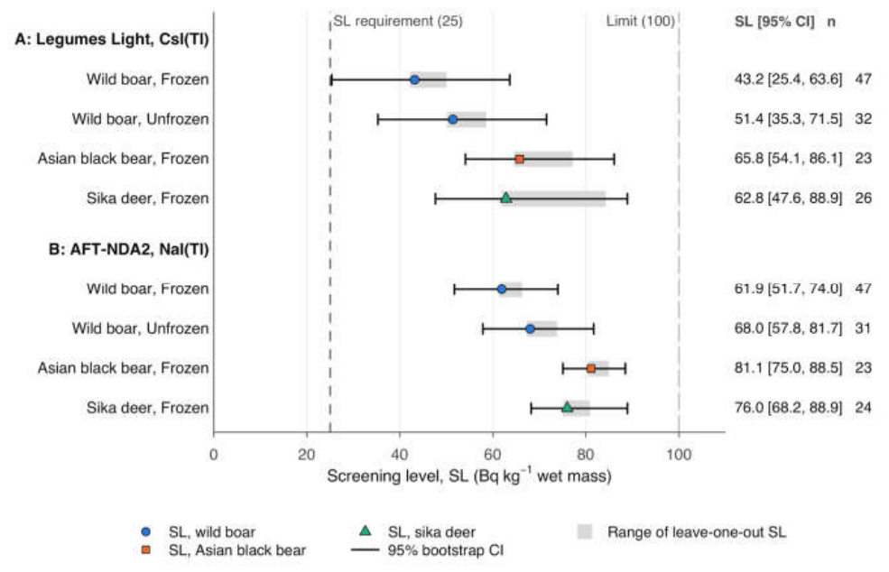
Screening levels (SL) obtained with the regression-based approach in the eight main strata. Symbols: point estimates; horizontal bars: individual-level bootstrap 95% percentile CIs (B = 2,000; seed 20261002 + stratum number); grey bands: range of the SL re-estimated with each calibration sample left out (all samples retained). Dashed line: SL requirement (25 Bq kg−1 wet mass); grey line: 100 Bq kg−1 wet mass. Values at right: SL [95% CI] and calibration n. CI end points are subject to bootstrap Monte Carlo variation; the lower bound for device A, wild boar, frozen (25.4 Bq kg−1 wet mass) lies close to the 25 Bq kg−1 wet mass requirement. Devices: A: Legumes Light (FD-08Cs1000-1), CsI(Tl); B: AFT-NDA2, NaI(Tl.
Figure 3.
Screening levels (SL) obtained with the regression-based approach in the eight main strata. Symbols: point estimates; horizontal bars: individual-level bootstrap 95% percentile CIs (B = 2,000; seed 20261002 + stratum number); grey bands: range of the SL re-estimated with each calibration sample left out (all samples retained). Dashed line: SL requirement (25 Bq kg−1 wet mass); grey line: 100 Bq kg−1 wet mass. Values at right: SL [95% CI] and calibration n. CI end points are subject to bootstrap Monte Carlo variation; the lower bound for device A, wild boar, frozen (25.4 Bq kg−1 wet mass) lies close to the 25 Bq kg−1 wet mass requirement. Devices: A: Legumes Light (FD-08Cs1000-1), CsI(Tl); B: AFT-NDA2, NaI(Tl.
2.9. Statistical Software
All computations were done in R 4.6.0 (R Core Team, 2026), using base functions (lm, qt, uniroot, binom.test, wilcox.test) and the packages nlme 3.1-169 (Pinheiro et al., 2026) and survival 3.8-6 (Therneau, 2026) (for interval-censored regression in S-ND2). Package versions were fixed with renv for reproducibility. The analysis scripts reproduce all tables and figures from the dataset (see Data availability). The authors designed the study, made the analysis decisions, interpreted the results, and take full responsibility for this work. Reported values were checked automatically against the final analysis outputs.
3. Results
3.1. Study Population and Analysis Sets
The analysis included 126 animals, yielding 364 animal–state–instrument records (Table 1; Figure 1). Ge-derived reference concentrations were higher in wild boar than in Asian black bear or sika deer (Table 1). In the eight main strata, 62 animals had reference concentrations above 100 Bq kg−1. These animals contributed 97 exceeding animal–state combinations (62 frozen and 35 unfrozen). Each combination was evaluated with both instruments, yielding 194 instrument-specific classification evaluations. For wild boar, 53 of 74 frozen and 35 of 50 unfrozen blocks exceeded the standard limit, and 33 and 22 lay between 50 and 250 Bq kg−1, the range around the standard limit. In contrast, exceedances were few among Asian black bear and sika deer, where only 4 of 24 and 5 of 27 blocks exceeded 100 Bq kg−1, and 9 and 7 lay between 50 and 250 Bq kg−1. Evaluation set records excluded from calibration regressions were restricted to samples with Ge concentrations above 250 Bq kg−1, samples with no detected reading, or the single animal without detectable 137Cs (Figure 1). No additional observations were discarded.
3.2. Screening Levels Under the MHLW Method
OLS calibration fits and the corresponding SL derivations for the eight main strata are shown in Figure 2, and the regression parameters are given in Table 2. Point estimates of SL ranged from 43.2 to 81.1 Bq kg−1 and met the ≥25 Bq kg−1 requirement in all eight main strata (Table 2; Figure 3). Bootstrap confidence intervals were wide in several strata. The lowest lower confidence limit, 25.4 Bq kg−1 (frozen wild boar measured with the Legumes Light; SL 43.2 Bq kg−1, 95% CI 25.4–63.6), was close to the 25 Bq kg−1 requirement. This limit may cross the requirement under Monte Carlo sampling variation. For every species and sample-state combination, the SL was higher for the AFT-NDA2 than for the Legumes Light.
Sensitivity to individual samples in leave-one-out re-estimation was greatest in the smaller strata (Figure 3; S-Figure 3; S-Table 10). For frozen sika deer measured with the Legumes Light, leaving out single animals gave re-estimated SLs of 61.8 to 84.3 Bq kg−1 (largest shift, 21.47 Bq kg−1). In the wild boar strata, the largest leave-one-out shift was 7.13 Bq kg−1. For unfrozen Asian black bear, the small number of samples allowed SL to be calculated only as an exploratory reference from 5 calibration samples. No solution could be obtained for unfrozen sika deer (2 calibration samples) (S-Table 4).
3.3. Classification Performance and Validation
No sample exceeding the 100 Bq kg−1 standard limit was classified as screen-negative in any of the eight main strata (0/194 instrument-specific classification evaluations of the 97 exceeding animal–state combinations; Table 3). For wild boar, the upper 95% confidence limit of the false-negative rate was 6.7% in the frozen state (0/53) and 10.0% in the unfrozen state (0/35), the same for both instruments. In contrast, for sika deer (0/5) and Asian black bear (0/4), the few exceeding samples gave upper 95% confidence limits of 52.2% and 60.2%, corresponding to lower 95% confidence limits of sensitivity of 47.8% and 39.8% (Table 3). Classification performance for bear and deer thus remains statistically unconfirmed. False-positive classifications were concentrated mainly among samples with intermediate concentrations between 50 and 100 Bq kg−1 (Table 3; S-Table 5).
Internal leave-one-out cross-validation gave a valid SL in every fold (0 failed folds). It produced no false-negative classifications among exceeding samples (0/194 instrument-specific classification evaluations; with the same upper 95% confidence limits as the primary evaluation) and the same false-positive counts as the primary evaluation in all strata (Table 3).
In temporal validation for wild boar, thresholds calibrated from FY2023 samples classified FY2024 samples without false negatives (frozen: 0/20, upper 95% confidence limit 16.8%; unfrozen: 0/13, upper limit 24.7%; the same for both instruments; S-Table 6). Screening levels derived from FY2023 data alone were lower than full-data estimates, with differences of −21.8 to −12.9 Bq kg−1 in the four wild boar strata. For Asian black bear and sika deer, the FY2024 samples included only 0 and 2 exceeding samples, so a meaningful temporal evaluation was not possible.
Table 3.
Observed classification performance and individual-level leave-one-out validation in the eight main strata.
Table 3.
Observed classification performance and individual-level leave-one-out validation in the eight main strata.
| Device | Species | State | T_SL, Bq kg−1 | n (evaluation) | n > 100 | FN / n > 100 (95% upper bound) | FP / n ≤ 100 | Sensitivity [95% CI] | Specificity [95% CI] | LOO: FN / n > 100 (95% upper bound) | LOO: FP / n ≤ 100 | LOO: folds without SL |
| A: Legumes Light, CsI(Tl) | Wild boar | Frozen | 51.9 | 74 | 53 | 0/53 (upper 6.7%) | 9/21 | 100.0% [93.3%, 100.0%] | 57.1% [34.0%, 78.2%] | 0/53 (upper 6.7%) | 9/21 | 0 |
| A: Legumes Light, CsI(Tl) | Wild boar | Unfrozen | 70.1 | 50 | 35 | 0/35 (upper 10.0%) | 6/15 | 100.0% [90.0%, 100.0%] | 60.0% [32.3%, 83.7%] | 0/35 (upper 10.0%) | 6/15 | 0 |
| A: Legumes Light, CsI(Tl) | Asian black bear | Frozen | 64.1 | 24 | 4 | 0/4 (upper 60.2%) | 2/20 | 100.0% [39.8%, 100.0%] | 90.0% [68.3%, 98.8%] | 0/4 (upper 60.2%) | 2/20 | 0 |
| A: Legumes Light, CsI(Tl) | Sika deer | Frozen | 66.5 | 27 | 5 | 0/5 (upper 52.2%) | 2/22 | 100.0% [47.8%, 100.0%] | 90.9% [70.8%, 98.9%] | 0/5 (upper 52.2%) | 2/22 | 0 |
| B: AFT-NDA2, NaI(Tl) | Wild boar | Frozen | 53.6 | 74 | 53 | 0/53 (upper 6.7%) | 7/21 | 100.0% [93.3%, 100.0%] | 66.7% [43.0%, 85.4%] | 0/53 (upper 6.7%) | 7/21 | 0 |
| B: AFT-NDA2, NaI(Tl) | Wild boar | Unfrozen | 66.2 | 50 | 35 | 0/35 (upper 10.0%) | 3/15 | 100.0% [90.0%, 100.0%] | 80.0% [51.9%, 95.7%] | 0/35 (upper 10.0%) | 3/15 | 0 |
| B: AFT-NDA2, NaI(Tl) | Asian black bear | Frozen | 59.9 | 24 | 4 | 0/4 (upper 60.2%) | 0/20 | 100.0% [39.8%, 100.0%] | 100.0% [83.2%, 100.0%] | 0/4 (upper 60.2%) | 0/20 | 0 |
| B: AFT-NDA2, NaI(Tl) | Sika deer | Frozen | 60.4 | 27 | 5 | 0/5 (upper 52.2%) | 1/22 | 100.0% [47.8%, 100.0%] | 95.5% [77.2%, 99.9%] | 0/5 (upper 52.2%) | 1/22 | 0 |
Screen-positive: device indication > T_SL (Table 2); indications at or below T_SL and samples with all replicates not detected are screen-negative. True exceedance: Ge-derived 134Cs + 137Cs > 100 Bq kg−1 wet mass (Ge 137Cs not detected = 0). FN: exceeding samples classified screen-negative; FP: non-exceeding samples classified screen-positive. For FN = 0 the upper bound of the Clopper–Pearson 95% CI of the false-negative rate (1 − 0.025^(1/k), k = number of exceeding samples) is given; 0 observed false negatives does not mean a false-negative probability of 0. Sensitivity and specificity with Clopper–Pearson 95% CIs. LOO: individual-level leave-one-out cross-validation; for each sample the SL and T_SL were re-estimated without that sample, and the sample was then classified. PPV and NPV are not reported because the proportion of exceeding samples does not represent an inspection population. Model-based miss probabilities are reported separately (Table 4). Classification by concentration band and the pooled strata: S-Table 5; temporal validation (FY2023 to FY2024): S-Table 6. Devices: A: Legumes Light (FD-08Cs1000-1), CsI(Tl); B: AFT-NDA2, NaI(Tl).
Table 4.
Measurement-error structure and model-based miss probability at the device threshold (T_SL) in the eight main strata.
Table 4.
Measurement-error structure and model-based miss probability at the device threshold (T_SL) in the eight main strata.
| Device | Species | State | n (calibration) | Breusch–Pagan p | Slope of log|residual| on log fitted | Replicate CV, median (Ge ≥ 50) | Between-sample SD of log(device/Ge) (Ge ≥ 50) | θ, IRLS [95% CI]* | P_FN(100) at T_SL, IRLS [95% CI]* | IRLS non-converged resamples | P_FN(100), θ = 0 (OLS) | P_FN(100), θ = 1 | P_FN(100), log–log |
| A: Legumes Light, CsI(Tl) | Wild boar | Frozen | 47 | 0.007 | 0.89 | 5.6% | 0.170 | 0.77 [0.50, 1.53] | 0.12% [0.01%, 0.69%] | 228/2000 | 0.94% | 0.14% | 0.00% |
| A: Legumes Light, CsI(Tl) | Wild boar | Unfrozen | 32 | 0.010 | 1.63 | 2.8% | 0.148 | 1.59 [0.47, 2.33] | 0.43% [0.01%, 4.78%] | 356/2000 | 0.94% | 0.12% | 0.01% |
| A: Legumes Light, CsI(Tl) | Asian black bear | Frozen | 23 | <0.001 | 0.51 | 4.8% | 0.165 | 1.34 [0.12, 2.24] | 3.74% [0.34%, 36.08%] | 276/2000 | 1.05% | 0.91% | 0.42% |
| A: Legumes Light, CsI(Tl) | Sika deer | Frozen | 26 | <0.001 | 0.72 | 3.8% | 0.189 | 0.98 [-0.50, 1.55] | 4.60% [0.02%, 37.33%] | 370/2000 | 1.06% | 5.14% | 6.80% |
| B: AFT-NDA2, NaI(Tl) | Wild boar | Frozen | 47 | 0.001 | 0.84 | 7.1% | 0.104 | 0.86 [0.42, 1.54] | 0.18% [0.03%, 0.98%] | 177/2000 | 0.97% | 0.23% | 0.03% |
| B: AFT-NDA2, NaI(Tl) | Wild boar | Unfrozen | 31 | 0.014 | 1.12 | 5.0% | 0.092 | 0.99 [0.47, 2.04] | 0.10% [0.01%, 1.03%] | 323/2000 | 0.96% | 0.10% | 0.03% |
| B: AFT-NDA2, NaI(Tl) | Asian black bear | Frozen | 23 | 0.482 | 0.08 | 8.9% | 0.103 | 0.07 [-0.65, 1.01] | 1.26% [0.04%, 12.54%] | 296/2000 | 1.04% | 20.04% | 24.03% |
| B: AFT-NDA2, NaI(Tl) | Sika deer | Frozen | 24 | 0.041 | 0.09 | 4.0% | 0.165 | 0.44 [-1.18, 1.09] | 2.52% [0.00%, 16.50%] | 341/2000 | 1.05% | 13.30% | 11.61% |
Diagnostics on the calibration set: Breusch–Pagan test (Koenker) of the OLS residuals; slope of log|OLS residual| on log fitted value; median replicate CV and between-sample SD of log(device/Ge) among samples with four detected replicates and Ge ≥ 50 Bq kg−1 wet mass. θ: exponent of the prespecified variance-function model Var(e) = σ2μ^(2θ), fitted by IRLS (θ = 0: constant variance; θ = 1: proportional error). P_FN(100): model-based probability that a sample with a true concentration of 100 Bq kg−1 wet mass gives a device indication below the device threshold T_SL (Table 2) under the fitted error model. It is a model-based quantity, not an observed false-negative rate (observed classification: Table 3). * CIs of IRLS-based quantities are bootstrap percentile intervals computed from converged resamples only and are conditional on IRLS convergence; they are not interpreted as guaranteeing nominal 95% coverage (non-converged resamples are shown). Alternative error models: θ = 0 (homoscedastic OLS, the assumption of the regression-based approach), θ = 1 (proportional error), log–log regression. The post hoc gls(varPower) bootstrap (S-Table 8) is a computational robustness check for IRLS non-convergence and does not replace the prespecified IRLS analysis. Further variance-function model quantities (σ, SDs at 100 Bq kg−1 wet mass, VF-SL) are in S-Table 7. NC: not converged.Devices: A: Legumes Light (FD-08Cs1000-1), CsI(Tl); B: AFT-NDA2, NaI(Tl).
3.4. Measurement-Error Structure and Model-Based Miss Probability
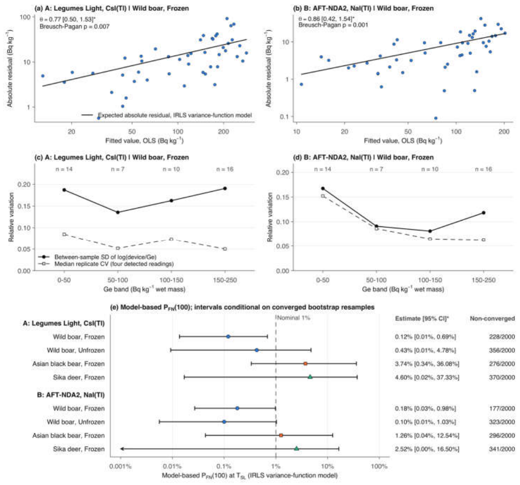
Residual diagnostics indicated significant heteroscedasticity in most strata: the studentized Breusch–Pagan test gave p < 0.05 in 7 of 8 main strata, and slopes of log |residual| on log fitted value were positive in all strata (0.08–1.63) (Table 4; Figure 4a–b; S-Figure 2). Nevertheless, the strength of evidence for concentration-dependent variance varied across strata. Evidence for heteroscedasticity was consistent in all four wild boar strata and in bear and deer measured with the Legumes Light. For bear and deer measured with the AFT-NDA2, the evidence was ambiguous or weak: Breusch–Pagan p-values were 0.482 and 0.041, log–log residual slopes were near zero (0.08 and 0.09), and estimated variance exponents were 0.07 and 0.44. In all eight main strata, between-sample variation (SD of log(/)) exceeded the median replicate CV (e.g., 0.170 versus 5.6% for frozen wild boar measured with the Legumes Light; Table 4; Figure 4c–d). This indicates that the dominant error component was sample-specific rather than replicate variation.
Point estimates of the variance-function exponent spanned 0.07 to 1.59 across strata. For wild boar, was estimated at 0.77 (frozen) and 1.59 (unfrozen) for the Legumes Light, and 0.86 and 0.99 for the AFT-NDA2, consistent with an approximately proportional error structure (). Bootstrap confidence intervals, conditional on converged resamples, are given in Table 4 (IRLS failed to converge in 177–370 of the 2,000 resamples per stratum).
Under the constant-variance assumption of OLS (), the model-based miss probability at the standard limit, PFN(100), ranged from 0.94% to 1.06% in all strata, close to 1% by construction. Under the fitted variance-function model, however, the model-based PFN(100) was below 1% in the four wild boar strata (0.10%–0.43%; Table 4; Figure 4e). In contrast, across the four bear and deer strata, the model-based PFN(100) exceeded 1% (1.26%–4.60%), with upper bootstrap limits, conditional on converged resamples, reaching 37.3%. These were the strata in which the local predictive SD at 100 Bq kg−1 under the variance-function model exceeded the pooled OLS residual standard deviation . This excess was larger for the Legumes Light than for the AFT-NDA2 (for Asian black bear, local SD of 20.97 versus = 11.72, compared to 5.35 versus = 4.99; S-Table 7).
Model-based miss probabilities also depended on the assumed error model. Across comparison models and post hoc gls fits, PFN(100) estimates for wild boar ranged from 0.00% to 0.97% (Table 4; S-Table 8). For Asian black bear and sika deer, however, the estimates were sensitive to the error model. Comparison models with fixed proportional error () or log–log scaling gave substantially higher miss probabilities than the fitted model in the two AFT-NDA2 strata, where the evidence for heteroscedasticity was weak (Table 4). Post hoc generalized least squares (gls) bootstrap estimation had no numerical failures (0 of 16,000 resamples) and placed the model-based PFN(100) on the same side of 1% as IRLS in all eight main strata (S-Table 8). Screening levels derived directly under the variance-function model (VF-SL) also did not give a 1% miss probability (S-Table 7; S-Figure 4).
Figure 4.
Measurement-error structure and model-based miss probability. (a, b) Absolute OLS residual versus fitted value (log–log) in the wild boar, frozen calibration sets of devices A and B, with the expected absolute residual under the prespecified variance-function model Var(e) = σ2μ^(2θ) fitted by IRLS; θ with its bootstrap interval (*) and the Breusch–Pagan (Koenker) p value. (c, d) Between-sample SD of log(device/Ge) and median replicate CV (samples with four detected readings) by Ge band in the same strata. (e) Model-based P_FN(100): probability, under the fitted variance-function model, that a sample with a true concentration of 100 Bq kg−1 wet mass gives a device indication below the device threshold T_SL of its stratum; it is a model-based quantity and not an observed false-negative rate (observed classification: Table 3). Dashed line: nominal 1%. Arrowheads mark interval limits below the axis range. Intervals of IRLS-based quantities are bootstrap percentile intervals computed from converged resamples only (B = 2,000; non-converged resamples per stratum shown) and are conditional on IRLS convergence; they are not interpreted as guaranteeing nominal 95% coverage. A post hoc gls(varPower) bootstrap was used only as a computational robustness check for IRLS non-convergence; it is not plotted and does not replace the prespecified IRLS analysis (S-Table 8). Non-converged resamples: A wild boar frozen 228/2000; A wild boar unfrozen 356/2000; A Asian black bear frozen 276/2000; A sika deer frozen 370/2000; B wild boar frozen 177/2000; B wild boar unfrozen 323/2000; B Asian black bear frozen 296/2000; B sika deer frozen 341/2000. Devices: A: Legumes Light (FD-08Cs1000-1), CsI(Tl); B: AFT-NDA2, NaI(Tl).
Figure 4.
Measurement-error structure and model-based miss probability. (a, b) Absolute OLS residual versus fitted value (log–log) in the wild boar, frozen calibration sets of devices A and B, with the expected absolute residual under the prespecified variance-function model Var(e) = σ2μ^(2θ) fitted by IRLS; θ with its bootstrap interval (*) and the Breusch–Pagan (Koenker) p value. (c, d) Between-sample SD of log(device/Ge) and median replicate CV (samples with four detected readings) by Ge band in the same strata. (e) Model-based P_FN(100): probability, under the fitted variance-function model, that a sample with a true concentration of 100 Bq kg−1 wet mass gives a device indication below the device threshold T_SL of its stratum; it is a model-based quantity and not an observed false-negative rate (observed classification: Table 3). Dashed line: nominal 1%. Arrowheads mark interval limits below the axis range. Intervals of IRLS-based quantities are bootstrap percentile intervals computed from converged resamples only (B = 2,000; non-converged resamples per stratum shown) and are conditional on IRLS convergence; they are not interpreted as guaranteeing nominal 95% coverage. A post hoc gls(varPower) bootstrap was used only as a computational robustness check for IRLS non-convergence; it is not plotted and does not replace the prespecified IRLS analysis (S-Table 8). Non-converged resamples: A wild boar frozen 228/2000; A wild boar unfrozen 356/2000; A Asian black bear frozen 276/2000; A sika deer frozen 370/2000; B wild boar frozen 177/2000; B wild boar unfrozen 323/2000; B Asian black bear frozen 296/2000; B sika deer frozen 341/2000. Devices: A: Legumes Light (FD-08Cs1000-1), CsI(Tl); B: AFT-NDA2, NaI(Tl).
3.5. Sensitivity and Robustness
Across the four alternative rules for non-detected readings, the SL values changed, but no false-negative classifications occurred in any main stratum (S-ND1 to S-ND4: 0 / 0 / 0 / 0; the upper 95% confidence limits were those of the primary evaluation). The largest change, −8.66 Bq kg−1, occurred when sub-25 Bq kg−1 readings were treated as non-detects (AFT-NDA2, sika deer, S-ND3; S-Table 9; S-Figure 4). Calibrating against recorded Ge totals shifted SL by at most −0.65 Bq kg−1 without inducing classification changes, while the alternative retest rule altered SL by at most 0.018 Bq kg−1.
The upper end of the calibration range had a large effect: an upper end of 200 Bq kg−1 changed SL by −0.8 to 20.5 Bq kg−1. Without an upper end, SL fell below the 25 Bq kg−1 requirement in 3 wild boar strata. False-positive classifications among frozen wild boar also increased to 21 with each instrument (compared with 9 and 7 in the primary analysis; S-Table 9). No false negatives occurred in any sensitivity analysis, so the upper 95% confidence limits were unchanged from the primary evaluation.
The most influential sample in the wild boar calibrations of the Legumes Light had a large positive residual but ordinary leverage. Retaining this sample lowered the SL (frozen blocks: 43.2 Bq kg−1 with versus 50.0 Bq kg−1 without the sample; S-Table 10). Additional sensitivity and exploratory analyses, including screening levels derived from fewer than four readings, are given in the Supporting Information (S-Table 11 to S-Table 15).
3.6. Effects of Sample State, Instrument and Species
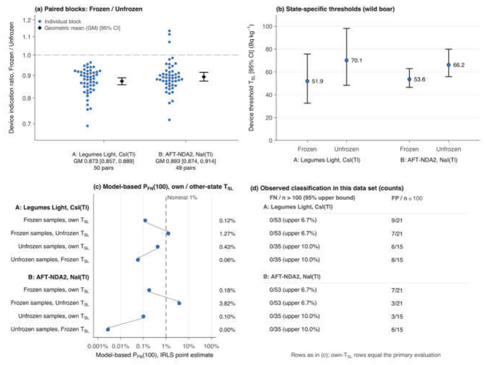
In the paired wild boar blocks, frozen blocks gave lower indications than the same blocks measured unfrozen, with both instruments. The geometric mean frozen-to-unfrozen ratio of indications was 0.873 (95% CI 0.857–0.889; 50 pairs) for the Legumes Light and 0.893 (0.874–0.914; 49 pairs) for the AFT-NDA2 (Wilcoxon signed-rank p < 0.001 for both instruments; Figure 5a; S-Table 12). Device thresholds () calibrated for frozen blocks were also lower than those for unfrozen blocks with both instruments (Figure 5b; Table 2).
When frozen samples were classified using the unfrozen-state thresholds (), no false negatives were observed (0/53 with each instrument; upper 95% confidence limit 6.7%), and false-positive classifications were fewer than with the frozen-state thresholds (Figure 5d; S-Table 12). Under the fitted frozen-state variance-function model, however, applying the unfrozen-state thresholds increased the model-based miss probability PFN(100) to 1.27% for the Legumes Light and 3.82% for the AFT-NDA2 (compared with 0.12% and 0.18% with the frozen-state thresholds; Figure 5c). Conversely, applying the frozen-state thresholds to unfrozen samples produced no observed false negatives (0/35; upper 95% confidence limit 10.0%) but more false positives. With the frozen-state thresholds, the model-based PFN(100) under the unfrozen-state variance-function model was lower than with the unfrozen-state thresholds (S-Table 12).
On the same samples, the Legumes Light gave higher indications than the AFT-NDA2, with geometric mean indication ratios of 1.178–1.395 across species and states and all 95% CIs above 1 (S-Table 13). Relative to the reference concentrations, the geometric mean ratio was 1.005–1.350 for the Legumes Light and 0.853–0.967 for the AFT-NDA2. Differences in residual dispersion between instruments had no uniform direction across species or states. The few classification disagreements between the two instruments did not involve exceeding samples (0 classification disagreements among exceeding samples; S-Table 13).
In the frozen samples, calibration relationships differed significantly among the three game species (species × concentration interaction, p = 0.005 for the Legumes Light and 0.007 for the AFT-NDA2). A single pooled screening threshold across species was therefore not supported (S-Table 14). An exploratory analysis examining block mass and the relative response of the Legumes Light is presented in S-Table 15.
Figure 5.
Unfrozen versus frozen wild boar thigh blocks (the same blocks measured before and after freezing). (a) Paired ratio of device indications, Frozen/Unfrozen (log scale), with the geometric mean (GM) and its individual-level bootstrap 95% CI (B = 2,000; seed 20261002 + 100 + stratum number). (b) Device threshold T_SL [95% bootstrap CI] estimated separately in each state. (c) Model-based P_FN(100) (IRLS point estimate under the variance-function model of the classified state) when samples are classified with the T_SL of their own state or with that of the other state; arrows connect the own-state and other-state values. (d) Observed classification of the same samples in this data set (counts): false negatives among exceeding samples (with the upper bound of the Clopper–Pearson 95% CI for 0) and false positives among non-exceeding samples. Panels (c) and (d) report different quantities: (c) is model-based and (d) is observed. Devices: A: Legumes Light (FD-08Cs1000-1), CsI(Tl); B: AFT-NDA2, NaI(Tl).
Figure 5.
Unfrozen versus frozen wild boar thigh blocks (the same blocks measured before and after freezing). (a) Paired ratio of device indications, Frozen/Unfrozen (log scale), with the geometric mean (GM) and its individual-level bootstrap 95% CI (B = 2,000; seed 20261002 + 100 + stratum number). (b) Device threshold T_SL [95% bootstrap CI] estimated separately in each state. (c) Model-based P_FN(100) (IRLS point estimate under the variance-function model of the classified state) when samples are classified with the T_SL of their own state or with that of the other state; arrows connect the own-state and other-state values. (d) Observed classification of the same samples in this data set (counts): false negatives among exceeding samples (with the upper bound of the Clopper–Pearson 95% CI for 0) and false positives among non-exceeding samples. Panels (c) and (d) report different quantities: (c) is model-based and (d) is observed. Devices: A: Legumes Light (FD-08Cs1000-1), CsI(Tl); B: AFT-NDA2, NaI(Tl).
4. Discussion
4.1. Principal Findings and Interpretation of Screening Levels
When applied to intact meat blocks of wild game, the regression-based approach of the MHLW method gave screening-level point estimates of at least 25 Bq kg−1 in all eight main strata. No sample exceeding the 100 Bq kg−1 standard limit was screened negative in the primary evaluation or in leave-one-out cross-validation, although the upper confidence limits of the false-negative rate depended on the number of exceeding samples in each stratum. However, residual measurement error increased with concentration in most strata and was dominated by sample-specific deviations rather than replicate variation. As a result, the false-negative control implied by the criterion was not fixed at the nominal ~1% baseline of homoscedastic regression theory. Evidence was comparatively robust for wild boar, which had many exceeding samples. In contrast, for Asian black bear and sika deer, the small number of exceeding samples leaves the classification performance largely unverified.
The requirement SL ≥ 25 Bq kg−1 is a condition for accepting a calibration rather than a guarantee of classification performance. In our data, SL was an estimate with considerable sampling uncertainty, and bootstrap intervals were wide. For frozen wild boar measured with the Legumes Light, the lower 95% confidence limit (25.4 Bq kg−1) was close to the 25 Bq kg−1 requirement. SL estimates were sensitive to single influential samples, to the restriction of the data to a single fiscal year, and, most strongly, to the upper end of the calibration range. While the upper end of our calibration range ( Bq kg−1) was prespecified to evaluate the regression-based approach, other choices of range produce substantially different thresholds. Because SL reflects the ratio of residual dispersion to calibration slope, it is an empirical property of a specific calibration set (instrument unit, geometry settings, sample population, and concentration range) rather than a constant of an instrument model or a food. This variability is also seen in the official worked examples, where published SL values differ widely across food types and instruments (MHLW, 2025; Yamada et al., 2023). Screening levels for operational use should therefore be reported with bootstrap confidence intervals and with leave-one-out and calibration-range diagnostics.
4.2. Error Structure and Interpretation of the 99% Prediction-Bound Framework
The MHLW screening criterion is defined by a 99% upper limit, which in the regression-based approach is a one-sided 99% prediction bound, and does not explicitly specify a target false-negative probability. In classical calibration theory, prediction limits on a response signal are constructed such that future observations fall outside them with defined small probabilities, corresponding to false-positive and false-negative decision risks (Hubaux and Vos, 1970). This interpretation assumes that measurement errors are normally distributed with constant variance. Under homoscedasticity, solving implies that a sample with a true concentration exactly at the 100 Bq kg−1 standard limit has an approximately 1% probability of giving an indication below , as our model-based estimates under showed (0.94%–1.06%). This nominal ~1% figure is our study's statistical interpretation rather than a regulatory target. The screening method for prepared foods allows the 99% upper limit to be obtained either from local replicate dispersion at the screening level or from global regression (MHLW, 2012a). The non-destructive method allows the same two approaches, and its worked examples use the global regression approach evaluated here (MHLW, 2025). In our intact meat data, however, residual variance increased with concentration in most strata and was dominated by between-sample variation rather than replicate variation. In studies of bagged wild mushrooms, Yamada et al. (2023) documented large replicate variability and large differences from Ge spectrometry at higher concentrations. They suggested that these arise from irregular item geometry and heterogeneous internal radiocaesium distributions rather than counting statistics. Because an intact meat block cannot be mixed or re-dispersed between readings (Section 2.2), we interpret this dominant between-sample variance as a deviation specific to each block that is not reduced by averaging repeated readings. This interpretation, however, was not directly tested.
When measurement variance increases with analyte concentration, the pooled residual standard deviation from an unweighted OLS regression does not represent the local dispersion at a given concentration, which distorts the prediction bounds. In chromatographic calibration, unweighted regressions gave distorted detection limits relative to variance-weighted models (Zorn et al., 1997). Because the regression-based approach uses a single pooled residual SD () over the whole calibration range, the miss probability at 100 Bq kg−1 depends on whether this pooled is larger or smaller than the local dispersion at the standard limit. In wild boar calibrations, which contained many samples with concentrations well above 100 Bq kg−1, the pooled exceeded the local predictive SD at 100 Bq kg−1 under the fitted variance-function model, and model-based miss probabilities were below 1%. In bear and deer calibrations measured with the Legumes Light, where most samples had low concentrations, the pooled was smaller than the local predictive SD at 100 Bq kg−1, and model-based miss probabilities exceeded 1%. In bear and deer measured with the AFT-NDA2, where evidence for heteroscedasticity was ambiguous, pooled and local SDs differed less, with smaller and less definitive departures of the model-based values from 1%. The strong dependence of SL on the upper end of the calibration range is consistent with this same mechanism: including high-concentration samples inflated the pooled residual variance, widening prediction bands and lowering SL.
These model-based miss probabilities have two limitations: their bootstrap confidence intervals are conditional on converged IRLS resamples, and the estimates for bear and deer were sensitive to the assumed error model (Section 3.4). They therefore indicate the direction in which heteroscedasticity affects false-negative control, rather than verified operational false-negative rates. Deriving screening levels directly under a variance-function model (VF-SL) also did not give a 1% miss probability, because the criterion places the prediction bound at SL rather than at the standard limit. Variance-function and weighted regression models are well established in analytical chemistry calibration (Davidian and Carroll, 1987; Zeng et al., 2008). Whether the screening criterion itself should be reformulated, for example by constraining the miss probability at the standard limit, is an open methodological question beyond the scope of this study.
4.3. Species-Dependent Uncertainty
The strength of the evidence differed between game species. For wild boar, the calibration sets contained many samples between 50 and 250 Bq kg−1, and no exceeding sample was misclassified (upper 95% confidence limits of 6.7% and 10.0%). Single samples had little influence on SL, and temporal validation produced no false negatives, even though thresholds calibrated from a single fiscal year were lower. In contrast, for Asian black bear and sika deer, only 4 and 5 exceeding samples were available. The absence of observed false negatives in these strata therefore remains compatible with substantial uncertainty in the underlying false-negative rate (upper 95% confidence limits of 60.2% and 52.2%). Leave-one-out re-estimation also shifted SL by up to 21.47 Bq kg−1, and the model-based values depended on the error model. Regression relationships also differed significantly among the three species, so a single pooled screening threshold was not supported. Screening levels derived for bear and deer meat should therefore be regarded as provisional.
4.4. Effects Of Sample State and Detector Characteristics
Paired measurements showed that frozen wild boar blocks gave lower indications than the same blocks measured unfrozen, so screening thresholds derived for one sample state should not be assumed to apply to the other. Applying the unfrozen-state thresholds to frozen samples produced no observed false negatives among 53 exceeding blocks (upper 95% confidence limit 6.7%). Under the fitted frozen-state variance-function model, however, applying the unfrozen-state thresholds increased the model-based miss probability at the 100 Bq kg−1 standard limit above the 1% nominal baseline. The opposite cross-application shifted classifications in a conservative direction at the cost of more false positives. Within the present data, these findings support calibrating screening thresholds separately for unfrozen and frozen meat. The physical mechanism responsible for the lower indications of frozen blocks was not investigated, and paired assessments were restricted to wild boar.
On the same samples, the Legumes Light gave higher indications than the AFT-NDA2, and calibrated SL values were higher for the AFT-NDA2 in all four species–state combinations. These differences reflect the responses of the individual instrument units under the settings used, rather than a general performance ranking of CsI(Tl) and NaI(Tl) scintillation detectors. The settings included the container-equivalent geometry setting of the Legumes Light and the mass input with preset densities of the AFT-NDA2. Because the regression-based approach calibrates indications empirically against reference Ge spectrometry, proportional offsets are absorbed into the regression slope and the device threshold.
4.5. Practical Scope and Limitations
Frozen-state measurements with the Legumes Light were an application outside the manufacturer's stated specimen condition. Empirical calibration against Ge spectrometry gave screening levels that describe the behaviour of this unit, but these thresholds are not supported by the manufacturer's specification and would require manufacturer confirmation or further verification before operational use. In addition, several blocks measured with the AFT-NDA2 were outside its specified 300–2,000 g mass range or lacked a mass entry (6 calibration records in the main strata). All were retained in accordance with our prespecified analysis plan. The MHLW method requires the sample mass range over which an SL is valid to be defined in advance (MHLW, 2025). The thresholds reported here apply to the mass distribution of the blocks studied.
The non-destructive instruments measured whole blocks weighing 171–2,860 g, whereas reference Ge spectrometry was performed on a homogenized subsample of 78.3–142.2 g wet mass cut from each block. The representativeness of the subsample for the whole block was not quantified. In radiocaesium analyses of beef, activity concentrations differed between muscle and fat and, to a lesser extent, between parts of a single block (Minatani et al., 2012). Uneven radiocaesium distribution within a block may thus account for part of the residual dispersion between indications and Ge results that is attributed here to instrument measurement error.
Wild game meat is not among the target foods of the MHLW screening method, and this study evaluated only its regression-based approach to the screening level. Other requirements of the method, such as daily energy calibration, routine function checks, and a standard operating procedure (MHLW, 2025), were outside the scope of this study and are only partly documented for these measurements. In the two-stage design of food screening, a false-positive result leads to confirmatory Ge spectrometry, whereas a false-negative classification is not corrected at a later stage. This asymmetry is why false-negative control matters.
Our findings derive from a single monitoring facility, one unit of each instrument model, and quadriceps femoris muscle blocks only. Differences between anatomical sites were not evaluated, and screening thresholds are specific to the instruments, settings, and sample distributions examined. Block mass, shape, and container settings were not controlled. Storage temperatures, freezing methods, and daily instrument checks before February 2024 were not documented. Some sub-25 Bq kg−1 readings came from the measurement workbook without instrument output files (examined in sensitivity analysis S-ND3). Temporal validation compared two consecutive fiscal years that may differ in capture areas and animal populations. Finally, potential false positives from naturally occurring radionuclides, which can confound scintillation screening spectra (Shozugawa et al., 2026), were not assessed. Measurement times other than the four-reading 600-s protocol and reproducibility between laboratories were also not assessed.
4.6. Implications
Within the conditions studied, we suggest that non-destructive screening thresholds for wild game meat be calibrated separately for each instrument, animal species, and sample state. Calibrations should include enough samples near the 100 Bq kg−1 standard limit and report bootstrap confidence intervals for SL, leave-one-out diagnostics, the sensitivity of SL to the calibration range, and an assessment of residual heteroscedasticity. For Asian black bear and sika deer, additional samples near the standard limit, collected prospectively and analysed separately from the present data, are needed before operational screening could be considered. In any operational use, non-destructive screening must serve only as the first stage of a two-stage inspection, with Ge spectrometry confirmation of screen-positive samples.
5. Conclusions
The regression-based approach of Japan's MHLW non-destructive method could be applied to intact quadriceps femoris muscle blocks of wild game from Fukushima Prefecture. Screening-level point estimates met the method's requirement of SL ≥ 25 Bq kg−1 in all eight instrument–species–state strata, and no sample exceeding the 100 Bq kg−1 standard limit was screened negative in the primary or leave-one-out evaluation. However, the upper confidence limits of the false-negative rate were wide for strata with few exceeding samples. Residual measurement error increased with concentration in most strata, and this error structure, together with the limited number of samples near and above the standard limit, affects confidence in the false-negative control implied by the criterion. Evidence was comparatively robust for wild boar, whereas findings for Asian black bear and sika deer remain provisional and require prospective calibration data near the standard limit. These findings provide a basis for further evaluation of non-destructive radiocaesium screening in wild game meat.
Funding
This work was supported by the Ministry of Health, Labour and Welfare, Japan, through 厚生労働科学研究費補助金(食品の安全確保推進研究事業)「食品中の放射性物質等検査システムの評価手法の開発に資する研究」 (grant number 23KA1006; sub-project 「食品中の放射性物質等検査システムの評価手法の検討」).
Data availability
The data are held by Fukushima Prefecture. Access is subject to approval by the prefecture.
Acknowledgments
The authors thank the members of the Fukushima Prefectural Hunters' Association for their assistance with sample collection. We also thank the technical staff of the Fukushima Prefectural Centre for Environmental Creation for sample preparation and germanium gamma-ray spectrometry.
Conflicts of Interest
The authors declare no competing interests.
References
- Bland, J.M., Altman, D.G., 1986. Statistical methods for assessing agreement between two methods of clinical measurement. The Lancet 327, 307–310. [CrossRef]
- Breusch, T.S., Pagan, A.R., 1979. A simple test for heteroscedasticity and random coefficient variation. Econometrica 47, 1287–1294. [CrossRef]
- Brown, M.B., Forsythe, A.B., 1974. Robust tests for the equality of variances. Journal of the American Statistical Association 69, 364–367. [CrossRef]
- Brynildsen, L.I., Strand, P., 1994. A rapid method for the determination of radioactive caesium in live animals and carcasses, and its practical application in Norway after the Chernobyl nuclear reactor accident. Acta Veterinaria Scandinavica 35, 401–408. [CrossRef]
- Carroll, R.J., Ruppert, D., 1988. Transformation and Weighting in Regression. Chapman and Hall, New York. [CrossRef]
- Clopper, C.J., Pearson, E.S., 1934. The use of confidence or fiducial limits illustrated in the case of the binomial. Biometrika 26, 404–413. [CrossRef]
- Cui, L., Orita, M., Taira, Y., Takamura, N., 2020. Radiocesium concentrations in wild boars captured within 20 km of the Fukushima Daiichi Nuclear Power Plant. Scientific Reports 10, 9272. [CrossRef]
- Davidian, M., Carroll, R.J., 1987. Variance function estimation. Journal of the American Statistical Association 82, 1079–1091. [CrossRef]
- Hachisuka, A., 2018. 食品中放射性物質の検査体制の評価手法の検討. In: 平成29年度 厚生労働行政推進調査事業費補助金(食品の安全確保推進研究事業)「食品中の放射性物質等検査システムの評価手法の開発に関する研究」総括・分担研究報告書, pp. 15–54. [Study on methods for evaluating the inspection system for radioactive materials in foods; sub-report of an MHLW-funded research project, fiscal year 2017] (in Japanese). https://mhlw-grants.niph.go.jp/system/files/download_pdf/2017/201723031A.pdf (accessed 12 October 2026).
- Hayashi, C., Nakamura, K., Hongo, T., Hashimoto, H., Harada, R., Nakanishi, K., Ishii, T., 2016. Surveillance of radioactive cesium in meats of wild animals caught in Chiba Prefecture. Food Hygiene and Safety Science (Shokuhin Eiseigaku Zasshi) 57, 32–36. (in Japanese with English abstract) . [CrossRef]
- Hubaux, A., Vos, G., 1970. Decision and detection limits for linear calibration curves. Analytical Chemistry 42, 849–855. [CrossRef]
- Ishii, K., 2015. 食品の汚染検査のための放射能非破壊検査装置. Isotope News No. 729, 21–27. [Non-destructive radioactivity inspection device for contamination testing of foods] (in Japanese).
- Ishii, K., 2018. ベルトコンベヤー式非破壊放射性セシウム汚染検査機. Radioisotopes 67, 67–73. [Belt-conveyor type non-destructive radioactive caesium contamination monitoring machine] (in Japanese). [CrossRef]
- Koenker, R., 1981. A note on studentizing a test for heteroscedasticity. Journal of Econometrics 17, 107–112. [CrossRef]
- Koganezawa, M., Okuda, K., Fukui, E., 2019. Radioactive cesium contamination of sika deer in Oku-Nikko region of Tochigi Prefecture in central Japan. In: Takenaka, C., Hijii, N., Kaneko, N., Ohkubo, T. (Eds.), Radiocesium Dynamics in a Japanese Forest Ecosystem. Springer, Singapore, pp. 195–200. [CrossRef]
- Komatsu, H., Ikushima, S., 2026. Factors affecting log-transformed muscle 137Cs concentrations in wild boars in Fukushima Prefecture over 14 years. PLOS ONE 21, e0344189. [CrossRef]
- Maekawa, A., Kanda, K., Murakami, K., Komatsu, H., Inoue, H., Hashimoto, K., 2024. 非破壊式放射能測定装置による野生鳥獣肉の放射性セシウムスクリーニング検査. In: 第5回日本放射線安全管理学会・日本保健物理学会合同大会 予稿集 [Abstracts of the 5th joint meeting of the Japanese Society of Radiation Safety Management and the Japan Health Physics Society], Osaka, 16–18 December 2024, abstract 1P29. [English title in the abstract: Screening for radioactive cesium in wildlife meat using non-destructive radioactivity measuring equipment] (in Japanese).
- Meredith, R.C.K., Mondon, K.J., Sherlock, J.C., 1988. A rapid method for the in vivo monitoring of radiocaesium activity in sheep. Journal of Environmental Radioactivity 7, 209–214. [CrossRef]
- Minatani, T., Nagai, H., Nakamura, M., Otsuka, K., Sakai, Y., 2012. Radioactive cesium analysis in radiation-tainted beef by gamma-ray spectrometry with germanium semiconductor detector. Food Hygiene and Safety Science (Shokuhin Eiseigaku Zasshi) 53, 177–182. (in Japanese with English abstract) . [CrossRef]
- Ministry of Health, Labour and Welfare (MHLW), 2012a. 食品中の放射性セシウムスクリーニング法の一部改正について. [Revision of the screening method for radioactive caesium in foods; administrative notice, 1 March 2012] (in Japanese). https://www.mhlw.go.jp/stf/houdou/2r985200000249rb-att/2r985200000249sz.pdf (accessed 3 October 2026).
- Ministry of Health, Labour and Welfare (MHLW), 2012b. 食品中の放射性物質の試験法について. [Test method for radioactive materials in foods; notification Shoku-An-Hatsu 0315 No. 4, 15 March 2012, with the attachment “食品中の放射性セシウム検査法”] (in Japanese). https://www.mhlw.go.jp/shinsai_jouhou/dl/shikenhou_120316.pdf (accessed 3 October 2026).
- Ministry of Health, Labour and Welfare (MHLW), 2012c. 乳及び乳製品の成分規格等に関する省令の一部を改正する省令、乳及び乳製品の成分規格等に関する省令別表の二の(一)の(1)の規定に基づき厚生労働大臣が定める放射性物質を定める件及び食品、添加物等の規格基準の一部を改正する件について. [Notice on the standard limits for radioactive caesium in foods; notification Shoku-An-Hatsu 0315 No. 1, 15 March 2012] (in Japanese). https://www.mhlw.go.jp/shinsai_jouhou/dl/tuuchi_120316.pdf (accessed 3 October 2026).
- Ministry of Health, Labour and Welfare (MHLW), 2015. 食品中の放射性物質に係る基準値の設定に関するQ&Aについて. [Q&A on the standard limits for radioactive materials in foods; notice of 5 July 2012, first revision 20 March 2015] (in Japanese). https://www.mhlw.go.jp/shinsai_jouhou/dl/120412_2.pdf (accessed 3 October 2026).
- Ministry of Health, Labour and Welfare (MHLW), 2023. 非破壊検査法による食品中の放射性セシウムスクリーニング法について. [Screening method for radioactive caesium in foods by non-destructive inspection; administrative notice of 30 March 2023 (first issued 26 March 2021)] (in Japanese).
- Ministry of Health, Labour and Welfare (MHLW), 2024. 非破壊検査法による食品中の放射性セシウムスクリーニング法について. [Screening method for radioactive caesium in foods by non-destructive inspection; administrative notice of 1 July 2024 (first issued 26 March 2021)] (in Japanese).
- Ministry of Health, Labour and Welfare (MHLW), 2025. 非破壊検査法による食品中の放射性セシウムスクリーニング法について. [Screening method for radioactive caesium in foods by non-destructive inspection; administrative notice of 28 August 2025 (first issued 26 March 2021)] (in Japanese). https://www.mhlw.go.jp/content/001551127.pdf (accessed 3 October 2026).
- Morgan, W.A., 1939. A test for the significance of the difference between the two variances in a sample from a normal bivariate population. Biometrika 31, 13–19. [CrossRef]
- Nakamura, K., Chiba, S., Kiuchi, T., Nabeshi, H., Tsutsumi, T., Akiyama, H., Hachisuka, A., 2022. Comprehensive analysis of a decade of cumulative radiocesium testing data for foodstuffs throughout Japan after the 2011 Fukushima Daiichi Nuclear Power Plant accident. PLOS ONE 17, e0274070. [CrossRef]
- Nemoto, Y., Saito, R., Oomachi, H., 2018. Seasonal variation of Cesium-137 concentration in Asian black bear (Ursus thibetanus) and wild boar (Sus scrofa) in Fukushima Prefecture, Japan. PLOS ONE 13, e0200797. [CrossRef]
- Nuclear Emergency Response Headquarters (NERHQ), 2024. 検査計画、出荷制限等の品目・区域の設定・解除の考え方. Nuclear Emergency Response Headquarters, Government of Japan, Tokyo. [Concepts of Inspection Planning and the Establishment and Cancellation of Items and Areas to which Restriction on Distribution and/or Consumption of Foods Concerned Applies (official English title of the guideline); revision of 26 March 2024] (in Japanese). https://www.mhlw.go.jp/content/11135000/001233140.pdf (accessed 3 October 2026).
- Pinheiro, J., Bates, D., R Core Team, 2026. nlme: Linear and Nonlinear Mixed Effects Models. R package version 3.1-169. [CrossRef]
- Pitman, E.J.G., 1939. A note on normal correlation. Biometrika 31, 9–12. [CrossRef]
- R Core Team, 2026. R: A Language and Environment for Statistical Computing. R Foundation for Statistical Computing, Vienna, Austria. Version 4.6.0. [CrossRef]
- Saito, R., Kumada, R., Inami, K., Kanda, K., Kabeya, M., Tamaoki, M., Nemoto, Y., 2022. Monitoring of radioactive cesium in wild boars captured inside the difficult-to-return zone in Fukushima Prefecture over a 5-year period. Scientific Reports 12, 5667. [CrossRef]
- Shozugawa, K., Hori, M., Takizawa, T., Thomas, J.E., 2026. Misidentification of natural and anthropogenic radionuclides in scintillation-based screening in Fukushima, Japan. Journal of Radioanalytical and Nuclear Chemistry 335, 759–765. [CrossRef]
- Stäger, F., Zok, D., Schiller, A.-K., Feng, B., Steinhauser, G., 2023. Disproportionately high contributions of 60 year old weapons-137Cs explain the persistence of radioactive contamination in Bavarian wild boars. Environmental Science & Technology 57, 13601–13611. [CrossRef]
- Steinhauser, G., Saey, P.R.J., 2016. 137Cs in the meat of wild boars: a comparison of the impacts of Chernobyl and Fukushima. Journal of Radioanalytical and Nuclear Chemistry 307, 1801–1806. [CrossRef]
- Therneau, T.M., 2026. A Package for Survival Analysis in R. R package version 3.8-6. https://CRAN.R-project.org/package=survival.
- Whiteside, T.S., Brand, A.D., Aucott, T.J., DiPrete, D.P., 2020. Improved field-portable system to measure Cs-137 in wildlife. Journal of Environmental Radioactivity 223–224, 106394. [CrossRef]
- Yamada, T., Kikuchi, M., Yagihashi, D., Yamakawa, S., Ishizu, H., Shiina, T., 2017. Screening test for radioactivity of self-consumption products in Fukushima after the Fukushima Dai-ichi NPP accident in Japan. Applied Radiation and Isotopes 126, 93–99. [CrossRef]
- Yamada, T., Soga, K., Hachinohe, M., Hachisuka, A., 2019. Performance evaluation of the equipment for measuring radioactivity in whole foodstuffs without destructive sample preparation developed after the Fukushima NPP accident. Radiation Protection Dosimetry 184, 355–358. [CrossRef]
- Yamada, T., Furutaka, K., Hachinohe, M., Hachisuka, A., 2023. Applicability of non-destructive equipment for radioactivity measurement to screening radio-cesium in foods. Applied Radiation and Isotopes 194, 110671. [CrossRef]
- Yamada, T., 2025. 食品中の放射性物質等検査システムの評価手法の検討. In: 令和6年度 厚生労働科学研究費補助金(食品の安全確保推進研究事業)「食品中の放射性物質等検査システムの評価手法の開発に資する研究」(23KA1006) 研究分担報告書, pp. 26–143. [Study on evaluation methods for inspection systems for radioactive materials in foods; sub-report of an MHLW-funded research project, fiscal year 2024] (in Japanese). https://mhlw-grants.niph.go.jp/system/files/report_pdf/202423016A-buntan1.pdf (accessed 12 October 2026).
- Zeng, Q.C., Zhang, E., Dong, H., Tellinghuisen, J., 2008. Weighted least squares in calibration: estimating data variance functions in high-performance liquid chromatography. Journal of Chromatography A 1206, 147–152. [CrossRef]
- Zorn, M.E., Gibbons, R.D., Sonzogni, W.C., 1997. Weighted least-squares approach to calculating limits of detection and quantification by modeling variability as a function of concentration. Analytical Chemistry 69, 3069–3075. [CrossRef]
Disclaimer/Publisher’s Note: The statements, opinions and data contained in all publications are solely those of the individual author(s) and contributor(s) and not of MDPI and/or the editor(s). MDPI and/or the editor(s) disclaim responsibility for any injury to people or property resulting from any ideas, methods, instructions or products referred to in the content. |
© 2026 by the authors. Licensee MDPI, Basel, Switzerland. This article is an open access article distributed under the terms and conditions of the Creative Commons Attribution (CC BY) license (http://creativecommons.org/licenses/by/4.0/).
Copyright: This open access article is published under a Creative Commons CC BY 4.0 license, which permit the free download, distribution, and reuse, provided that the author and preprint are cited in any reuse.