

Submitted:
11 November 2026
Posted:
12 November 2026
Read the latest preprint version here
Abstract
Sen predicted that the protected indices of single-centred black holes in type II string theory on T6 and T5 are positive. We prove this for every charge whose index is known: four-dimensional dyons, five-dimensional rotating black holes, and five-dimensional black holes of fixed angular momentum.
Keywords:
black hole microstates
; helicity trace index
; Jacobi forms
MSC: 11F50 (primary); 11P82; 81T30; 83E30
1. Introduction
The entropy of a supersymmetric black hole in string theory can be compared with a count of microscopic states. Strominger and Vafa did this for five-dimensional black holes made of D1- and D5-branes with momentum [34], Breckenridge, Myers, Peet and Vafa added angular momentum [7], and Maldacena, Moore and Strominger found the exact count for type II string theory on a torus [21]. In four dimensions the analogous formula was derived by Shih, Strominger and Yin from the relation between four- and five-dimensional black holes [17,33], and Sen extended it to all charges of a certain primitivity type [27,30]. These formulae count the states with a sign: what is computed at weak coupling is a helicity trace index, the quantity that does not change when the coupling is increased until the black hole forms [3,4,20,26].
A black hole is more than the integer that counts it. Sen observed that a single-centred black hole whose only hair outside the horizon are the zero modes of the broken supersymmetries has a horizon of zero angular momentum, so that its microstates all contribute to the index with the same sign. Once the zero modes are removed, the index must therefore be a positive integer [10,14,31]. For the black holes of type II string theory on the multi-centred configurations that could spoil this do not contribute [27,30], so the prediction applies to the microscopic formula itself. It is a nontrivial statement about Fourier coefficients: the formulae are sums of coefficients of the Jacobi form , whose signs alternate.1 Bringmann and Murthy stated the prediction for the four- and five-dimensional black holes of type II on and and proved it when the index is a single Fourier coefficient [8]. Sen introduced the five-dimensional index at fixed angular momentum [32], which the same argument predicts to be positive [8].
This paper proves the prediction in full, for every charge for which the index is known.
The indices
Write and , and define the integers by
so that , , , , , , and when or . The left side is the weak Jacobi form of weight and index 1 [16]; Section 2 explains why a coefficient depends only on .
In type IIB on , consider D1-, D3- and D5-branes wrapped on with charge vector Q and on with charge vector P; both lie in the even lattice of signature formed by the even homology of , and , , are the intersection products [30]. Put
A black hole with these charges exists when ; its entropy is [19]. When the index of the states with charges is [30]2
In type IIB on , a system of D1-branes and D5-branes with n units of momentum along and angular momentum forms a rotating five-dimensional black hole when ; its entropy is [7]. Put and, for ,
Results
Theorem A.
Let be charges with and . Then .
Theorem B.
Let with , and with . Then .
Theorem C.
Under the hypotheses of Theorem B with , .
The three statements are exactly the predictions of [8] and [32]. They cover every charge for which an exact formula is known; the four-dimensional charges with remain outside, see Section 8.3.
What the proof has to overcome
The sign of is (Lemma 2), and because the lattice is even. So the term of (2) is . If s is odd then and , so every odd s contributes a positive term as well; this is the observation behind the proofs of [8]. An even s breaks it. Take and , for instance and in two hyperbolic planes with . Then , , , and
The term is negative. Positivity is then a matter of size: the negative terms must be smaller than the positive ones, for every and every . In five dimensions the same problem appears in three places: in the divisor sum; in the difference (5), where two coefficients of the same sign are subtracted from each other; and at the values of l with , where the term of (3) survives and can carry either sign.
Plan
The proof rests on one inequality, Proposition 1: the growth of the coefficients within a residue class exceeds twice every divisor sum with . Section 2 collects the background and derives the facts about helicity traces, charge invariants and that the proof uses. Section 3 writes through the numbers of partitions of n into parts of six colours; this gives monotonicity and an upper bound. Section 4 proves explicit bounds for from above and below. Section 5 proves the inequality, analytically for and by finite arithmetic below. Section 6 and Section 7 prove the three theorems and work out examples. Section 8 discusses sharpness, the U-duality invariant extension of [21] and the charges not covered by (2). Appendix A derives the elementary facts used along the way, and Appendix B describes the finite computation.
2. Background
2.1. Helicity Traces and Fermion Zero Modes
Let h be the helicity, the eigenvalue of the rotation generator in the rest frame of a massive particle in four dimensions. The helicity traces are
the trace running over the states of fixed charge [3,4,20]. A BPS state that breaks of the supercharges carries pairs of fermion zero modes, the goldstinos of the broken supersymmetries. Each pair acts as a fermionic oscillator that raises h by , so it multiplies by for some , or, after a shift of the helicity and a sign that do not affect the argument, by .4 Hence
where is the trace over the remaining degrees of freedom. Since vanishes to first order at and there, every with vanishes, and in at only the term in which each derivative falls on a different zero-mode factor survives. There are such terms, so
For type II string theory on there are 32 supercharges, a quarter-BPS black hole preserves 4 of them and breaks 28, so and the relevant index is [26,30]. It is the first trace that does not vanish, it is protected, and is the index (2). In five dimensions the same reasoning applied to the four zero modes that carry gives the factor of (4) [14].
2.2. Why the Sign Is Predicted
At strong coupling the states counted by live on the horizon of the black hole. Sen showed, by the quantum entropy function [28,29], that a single-centred BPS black hole has a near horizon geometry whose isometry forces the horizon degrees of freedom to carry [14,31]. Then on all of them, and the trace equals the dimension of the space of horizon states, up to the overall sign fixed by the conventions. Chowdhury, Garavuso, Mondal and Sen tested this at weak coupling, finding that the microstates of D-brane systems with small charges all have zero angular momentum [9,10]. The prediction therefore reads in four dimensions; in five dimensions, where the horizon of the rotating black hole carries , it reads for the index summed over and for the index at fixed [32]. The large charge behaviour, , agrees with the black hole entropy, including the logarithmic corrections [13,32].
2.3. Charges and Their Invariants
The charges transform under T-duality, the integral automorphisms g of the lattice, by , and under S-duality by with ; both are part of the U-duality group [12,30].
Lemma 1.
Δ, and are invariant under T- and S-duality.
Proof.
Put , a binary quadratic form with integer coefficients. Its discriminant is , and is the greatest common divisor of its coefficients. T-duality preserves inner products, so it fixes f. S-duality replaces by , an invertible integral change of variables; this preserves the discriminant, and the content of a form divides the content of any form obtained from it by an integral substitution, so applying the inverse substitution shows that the content is unchanged.
For , let be the vector of minors . Under T-duality , where is an integral matrix with integral inverse ; such a matrix preserves the greatest common divisor of the entries of a vector, by the same divisibility argument. Under S-duality . □
2.4. The Jacobi form
The odd theta function and the Dedekind eta function are
This is a weak Jacobi form of weight and index 1 [16]. For index one, invariance under forces the coefficient of to depend only on and on , which is determined by D; this is the reason for writing the coefficients as . Lemma 2 below proves this directly. Grouping the terms by gives the theta decomposition
2.5. The Five-Dimensional Generating Function
The D1-D5 system wrapped on is described at low energy by a two-dimensional conformal field theory, and the generating function of its BPS states is built from the elliptic genus of a symmetric product [15,21]. After the four fermion zero modes are removed, the coefficient of in the relevant generating function is of (3), and the index is (4) [14]. The relation between the four- and five-dimensional black holes [17] identifies J with the momentum along the circle of a Taub-NUT space, and the same coefficients appear in both indices. Expanding the factor
and comparing coefficients of gives (4). Since and the binomial coefficients are symmetric, .
3. The Coefficients
Let
so that counts the partitions of n into parts of six colours, and put for . The values for are listed in Table A1.
Lemma 2.
For every with ,
In particular , and
Proof.
By the definition of ,
Hence the coefficient of in (1) is , summed over half-integers with . Put . Then , the argument of a becomes with , the pairs correspond to the integers , and . Since , the sign is and the parity condition is . This proves (9); the term or is at least . For the integers j are even, , and ; for they are odd, , and , the values t and giving the same term. □
In generating function form the lemma says and , which is (8). Figure 1 shows the coefficients and their alternating sign.
Lemma 3.
The sequence is nondecreasing, and for ; also . For with put and . Then
In particular is strictly increasing on each of the classes and , . Moreover, for every ,
Proof.
The series has nonnegative coefficients, and since the second factor has constant term 1, its coefficient of is at least the coefficient of ; hence for . In the same way gives . For , Lemma 2 gives
a sum of nonnegative terms whose term is . For the same computation with in place of and the factor 2 gives the second case. In (9) the integers j of fixed parity with lie in an interval of length with spacing 2, so there are at most of them, and each argument of a is at most ; since a is nondecreasing, (11) follows. □
Two arithmetic facts link the charges with these coefficients.
Lemma 4.
Let lie in an even lattice with integral bilinear form, and let and Δ be as in Section 1. Then , , and and . If , then for every .
Proof.
and are even, so and , which is and or because a square is 0 or 1 modulo 4. Writing shows . Let L be the Gram matrix in a basis of the lattice, so that . By Lagrange’s identity (Appendix A) applied to the vectors ,
where the dot is now the Euclidean product of coordinate vectors. The vector has entries that are integral combinations of the entries of . Both factors are divisible by , so . If then , and every divisor s of has . □
4. Partitions into Six Colours
The proof needs bounded above at about half the argument and below at the full argument, with explicit constants. Figure 2 shows the bounds of this section against the true values.
Lemma 5.
For every ,
Proof.
For the transformation [2] gives
Indeed by the definition of , and . Since the coefficients of P are nonnegative, . Take : then , and . With ,
so the product raised to the power is at most . The second bound is for ; for , . Appendix A gives a proof of the second bound that does not use the transformation of . □
Lemma 6.
Let be the coefficients of , that is,
Then for all , and for .
Proof.
Logarithmic differentiation of and of gives
where is the sum of the divisors of i; indeed . Since and , induction on n gives . The closed form follows from with and .
For the lower bound let , and ; note . Keeping one term,
Robbins’ form of Stirling’s formula [24] is . It gives , and so
because and therefore . For we have (Appendix A), and . Since and ,
Altogether . The three last terms decrease in n; at they are , and , and . The exponent is therefore at least . □
Lemma 7.
For , .
Proof.
Let be the coefficients of . Then and , so
Since for , the claim follows. □
Combining (10) with Lemmas 6 and 7: for , and ,
5. The Key Inequality
For put
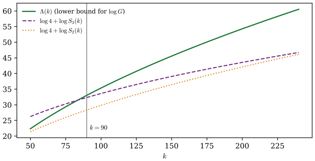
and for . So bounds every divisor sum with .
Proposition 1.
For every with ,
Proof.
The range . Here and . Let . Every term of has , and by (11) it is at most , which increases with E. The term is therefore at most
by Lemma 5 and because increases for (its logarithmic derivative is ), evaluated at . For the factors and are largest at , and , since . With the second bound of Lemma 5,
At ,
For the derivatives, . Differentiating the logarithms and discarding the negative terms,
For the derivative of is . For the derivative of is , and with the derivative of is . Hence
all positive for . So (15) holds for every .7
The range . Here every quantity in (13) and (14) is an integer determined by through (9). Appendix B describes the computation, which compares integers only. Both inequalities hold; the largest value of is , at , and the largest value of is , at , where and . Figure 3 shows both ratios. □
Figure 3.
The two ratios of Proposition 1 for . Both stay below 1, with the largest values at the smallest discriminants, and fall off like .
Figure 3.
The two ratios of Proposition 1 for . Both stay below 1, with the largest values at the smallest discriminants, and fall off like .
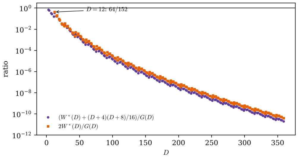
Figure 4.
The lower bound for against the upper bounds for the divisor sums. The analytic argument applies from on.
Figure 4.
The lower bound for against the upper bounds for the divisor sums. The analytic argument applies from on.
The inequality is used in the following form.
Corollary 1.
Let with , and let , for the integers with , be real numbers with and . Then
Proof.
The term is by Lemma 2, and the others add up to at most in absolute value. By (13), . □
6. Four-Dimensional Dyons
Proof of Theorem A.
By Lemma 4, , so forces ; for every ; and . Hence
and , . Corollary 1 gives . □
The proof uses neither the parity of s nor the sign of ; only enters, and the weights of (2) are smaller by a factor s. By Lemma 1 the index depends on the charges only through , and the parity of , which is the parity of .
Table 1 lists the index for small charges in Sen’s normal form of Section 2.3, realised as , in two hyperbolic planes, so that , , , and is primitive because its entry is 1. The terms of (2) are listed with their signs. A negative term occurs exactly when s is even and has the parity opposite to , as for with and with ; in every case it is a tiny fraction of the leading term. Figure 5 shows the growth of the index.8
7. Five-Dimensional Black Holes
Fix with , put and , and for write and
with F as in (3). If then and , so ; if moreover , then . Since , is an even function of l. Note that and .
Lemma 8.
- 1.
- If , then .
- 2.
- If , then ; if , then .
- 3.
- If , then when with and , and otherwise. In the first case , so for odd l and for even l.
Proof.
Since , (1) is Corollary 1 with for and otherwise. If then l is even and every contributes , so . If , only has , l is odd and . If , a term s of (3) is nonzero only if , that is ; since divides , this means . So there is at most one nonzero term, , present when is an integer dividing , and it equals . Finally . □
The values in (3) are the polar terms. They are nonzero only when , and they are small, but they enter (4) and (5) with fixed signs and have to be controlled. The next lemma ties their size to the discriminant of a nearby l.
Lemma 9.
Let with , and suppose with and . Put and . Then λ is odd, , and
where u is a positive integer with . In particular , and when is even.
Proof.
As noted above, gives ; put . Dividing by gives , so is odd and at least 3. Next,
which is the identity. Its left side is positive, so , and . If is even then . □
For example , , give and ; at , and . With we have , , and . Lemma 9 is sharp here. Figure 6 shows this charge.
Since , the definition (4) becomes
Proof of Theorem B.
Since is even in J, we may assume . Put ; then , because and . The term of (16) is by Lemma 8(1). The other terms have with . If the term is nonnegative by Lemma 8. If then , so with ; the term is negative only if is even and with even, and then, by Lemma 9 with and , it is at least . For the values are and , with coefficients 4 and 1; for the even ones are , with coefficients 1 and 1. In all cases
For the right side is and . For put ; then , and by Lemma 2 and Lemma 3, , since . So . □
In the index at fixed J the terms no longer have the same sign, and the monotonicity of the coefficients has to absorb the difference.
Lemma 10.
Let with and .
- 1.
- If , then .
- 2.
- If and , then .
Proof.
Put and . Then is a product of two even numbers, both at least 2, so and . By Lemma 3, whenever .
(1) If , Lemma 8 and (13) give
If , then and .
If , then and with . Since , , so . With and (Appendix A),
and . The right side is positive by (14).
(2) By Lemma 8(3) we may assume , since otherwise . Then is odd, with odd, , and . Also is odd, so is odd and ; and . Lemma 9 gives .
Suppose and write with . For , . For , ; this is 63 at and grows by with each step, while is 51 at and grows by 4. In both cases .
Suppose . By Lemma 9, and with odd and , so is , or for . The products are for and for ; their factorisations have , , and , , . The only sums of the required form are and , both for , with and . Then , and for no polar value occurs. □
The case is the only place where a divisor sum enters with no small factor in front of it: all its terms carry the same sign as the leading term of , and they are subtracted. This is the reason for the second inequality of Proposition 1.
Proof of Theorem C.
By (5) and (16), collecting the coefficient of each ,
since the coefficients of are . Hence
using that is even. Put and . Then , the two numbers have the same parity, and is when and when . If then and . If then is , or and is 1, 2 or 1; here , and unless . In all these cases Lemma 10 shows that the bracket is positive. In the remaining case , , , the bracket is with and , which is not minus a square, so it equals . Every bracket is positive, and so is d. □
Table 2 lists the five-dimensional indices for small charges, together with three values for the charge , of Figure 6. At and the polar value enters (16) with coefficient 1 and lowers from 36446 to 36444; at and the polar value is subtracted with coefficient 1 in (5), against . Figure 7 shows the index at fixed J for ; at fixed M it decreases with J, in line with the pairing in the last proof.
8. Remarks
8.1. Sharpness
The divisor terms are exponentially smaller than the leading term for large discriminants: by Lemma 5 the term of is at most , while [30]. The content of Proposition 1 is that this separation already holds at the smallest discriminants, where it is tight: at the term takes 16 of the 208 units of the leading term in (2), and is of . The polar values are smaller still, at most linear in the discriminant by Lemma 9, but they are not negligible at small charges: the case , of Lemma 10 uses more than half of . The lower bound of Lemma 6 grows like instead of the true , which is why the analytic argument starts only at .
8.2. The U-Duality Invariant Extension
For charges with , Maldacena, Moore and Strominger proposed the U-duality invariant extension of (3) in which the divisor s carries the weight , with the number of common divisors of , the sum running over the s for which and all these quotients are integers [21]. For such charges , since a common divisor of is 1, so the weights again lie in , are even in l, and are supported on divisors s of l with . The proofs of Lemmas 8, 9 and 10 use nothing else: in Lemma 8(2) the value at becomes over a set of divisors of l, which is at most , and the bound is unchanged. Hence, if the extension holds, the indices it predicts satisfy Theorems B and C for every charge with .
8.3. Charges of Higher Torsion
For four-dimensional charges with no formula for the index has been established [30], and the theorems say nothing about them. Corollary 1 reduces their positivity to a structural statement: any index of the form with and is positive, whatever the signs of the other weights. Any future formula of this shape, with the divisor weights bounded by , would therefore give positive indices at once.9
Funding
None.
Data Availability Statement
All data that support the findings of this study are contained in the article: Table A1 lists the numbers used in the finite part of the proof, and Appendix B describes the verification. The program that repeats the verification, computes the tables and draws the figures is archived at doi:10.5281/zenodo.24122289.
Conflicts of Interest
None.
Ethics Statement
This study involves no human participants, animals or personal data; no ethical approval was required.
Appendix A Elementary Facts
Appendix Lagrange’s Identity
For vectors ,
Both sides are bilinear in and in , so it suffices to take basis vectors , , , . The left side is . On the right, the term is nonzero only if with , and it is then if and if . The two sides agree. In Lemma 4 this is applied with , , , , using because L is symmetric.
Appendix Two inequalities
For , the function has and , so . For the divisors of m are distinct elements of , so .
Appendix Jacobi’s triple product
For and ,
Appendix A bound for a(n) without modular forms
For ,
because . Hence , and the choice gives , the second bound of Lemma 5.
Appendix B The Finite Range
The inequalities (13) and (14) for involve integers only, and their verification consists of four steps.
- (F1)
- The numbers , , are computed from the recursion of Lemma 6, or equivalently by multiplying out six copies of ; they are listed in Table A1.
- (F2)
- For , is computed from (9).
- (F3)
- For , is computed from its definition, and as a running maximum.
- (F4)
- For each D in the range with , the integers , and are compared.
Table A2 lists the quantities for ; the margin grows rapidly, as Figure 3 shows. The same program checks, as controls that the proofs do not use: the formula (9) against the direct expansion of up to and against the product (7) up to ; the bounds of Section 4 for ; the conclusions of Theorems A to C by evaluating (2), (4) and (5) directly on 1722 four-dimensional charges in Sen’s normal form and 5750 five-dimensional charges; all 868 five-dimensional charges with in which a polar value enters, together with the bound of Lemma 9; and 3195 charges for the extension of [21].

Table A1.
The numbers of partitions of n into parts of six colours, .
| n | n | n | |||
|---|---|---|---|---|---|
| 0 | 1 | 31 | 30227301468 | 62 | 13799370667455450 |
| 1 | 6 | 32 | 49522366656 | 63 | 19845194082605218 |
| 2 | 27 | 33 | 80590617278 | 64 | 28465163415636075 |
| 3 | 98 | 34 | 130307480730 | 65 | 40724826208003224 |
| 4 | 315 | 35 | 209396014650 | 66 | 58118725494437321 |
| 5 | 918 | 36 | 334492740175 | 67 | 82738453811650308 |
| 6 | 2492 | 37 | 531278722086 | 68 | 117504789092547003 |
| 7 | 6372 | 38 | 839204245278 | 69 | 166487707267085750 |
| 8 | 15525 | 39 | 1318587244800 | 70 | 235346673673043703 |
| 9 | 36280 | 40 | 2061234013149 | 71 | 331935256651796730 |
| 10 | 81816 | 41 | 3206265612102 | 72 | 467129825087621531 |
| 11 | 178794 | 42 | 4963610011174 | 73 | 655963278944277444 |
| 12 | 380051 | 43 | 7648740634158 | 74 | 919173274601444100 |
| 13 | 788004 | 44 | 11733857681850 | 75 | 1285312714955089064 |
| 14 | 1597725 | 45 | 17923026108974 | 76 | 1793621662235878482 |
| 15 | 3174210 | 46 | 27262103713383 | 77 | 2497928656596353478 |
| 16 | 6190182 | 47 | 41299026921900 | 78 | 3471941462435113530 |
| 17 | 11867310 | 48 | 62316761884412 | 79 | 4816410159748817880 |
| 18 | 22395359 | 49 | 93670787579400 | 80 | 6668809352618868378 |
| 19 | 41650050 | 50 | 140276509484724 | 81 | 9216404411744168100 |
| 20 | 76413078 | 51 | 209311092717496 | 82 | 12713856676088969832 |
| 21 | 138421358 | 52 | 311221082489247 | 83 | 17506907536752046098 |
| 22 | 247783113 | 53 | 461164908282750 | 84 | 24064191719868828650 |
| 23 | 438616728 | 54 | 681072218736560 | 85 | 33019905786901987212 |
| 24 | 768291650 | 55 | 1002575819281092 | 86 | 45230951219325322689 |
| 25 | 1332444330 | 56 | 1471174898831406 | 87 | 61853350983484206818 |
| 26 | 2289213495 | 57 | 2152131323752182 | 88 | 84444293827166272965 |
| 27 | 3898064226 | 58 | 3138799331684016 | 89 | 115098208842781661400 |
| 28 | 6581591157 | 59 | 4564363803456240 | 90 | 156627966849287037846 |
| 29 | 11023247880 | 60 | 6618341988415724 | ||
| 30 | 18320981569 | 61 | 9569726912844018 |
Table A2.
The quantities of Proposition 1 for .
| D | D | ||||||||
|---|---|---|---|---|---|---|---|---|---|
| 3 | 8 | 7 | 0 | 0 | 35 | 69168 | 40269 | 0 | 224 |
| 4 | 12 | 10 | 0 | 0 | 36 | 85500 | 49412 | 108 | 224 |
| 7 | 39 | 31 | 0 | 0 | 39 | 159372 | 90204 | 0 | 224 |
| 8 | 56 | 44 | 0 | 0 | 40 | 195312 | 109812 | 0 | 224 |
| 11 | 152 | 113 | 0 | 0 | 43 | 355224 | 195852 | 0 | 224 |
| 12 | 208 | 152 | 32 | 32 | 44 | 431984 | 236672 | 608 | 608 |
| 15 | 513 | 361 | 0 | 32 | 47 | 768885 | 413661 | 0 | 608 |
| 16 | 684 | 476 | 48 | 48 | 48 | 928720 | 496736 | 960 | 960 |
| 19 | 1560 | 1047 | 0 | 48 | 51 | 1621296 | 852411 | 0 | 960 |
| 20 | 2032 | 1348 | 0 | 48 | 52 | 1946352 | 1017632 | 0 | 960 |
| 23 | 4382 | 2822 | 0 | 48 | 55 | 3339201 | 1717905 | 0 | 960 |
| 24 | 5616 | 3584 | 0 | 48 | 56 | 3986656 | 2040304 | 0 | 960 |
| 27 | 11552 | 7170 | 72 | 72 | 59 | 6732232 | 3393031 | 0 | 960 |
| 28 | 14592 | 8976 | 156 | 156 | 60 | 7997184 | 4010528 | 2052 | 2052 |
| 31 | 28899 | 17347 | 0 | 156 | 63 | 13311450 | 6579218 | 351 | 2052 |
| 32 | 36088 | 21496 | 224 | 224 |
References
- G. E. Andrews, The Theory of Partitions. In Encyclopedia of Mathematics and its Applications 2; Cambridge University Press: Cambridge, 1984. [CrossRef]
- Apostol, T. M. Modular Functions and Dirichlet Series in Number Theory. In Graduate Texts in Mathematics 41, 2nd ed.; Springer: New York, 1990. [Google Scholar] [CrossRef]
- Bachas, C.; Kiritsis, E. F4 terms in N=4 string vacua. Nucl. Phys. B Proc. Suppl. 1997, 55, 194–199. [Google Scholar] [CrossRef]
- Bachas, C.; Fabre, C.; Kiritsis, E.; Obers, N. A.; Vanhove, P. Heterotic/type-I duality and D-brane instantons. Nucl. Phys. B 1998, 509, 33–52. [Google Scholar] [CrossRef]
- Bhattacharjee, D. Generalization of quartic and quintic Calabi–Yau manifolds fibered by polarized K3 surfaces. Res. Sq. 2022. [Google Scholar] [CrossRef] [PubMed]
- Bhattacharjee, D.; Nandi, P. Enriques and Kummer surfaces arising from K3 involutions; Preprints, 2026. [Google Scholar] [CrossRef]
- Breckenridge, J. C.; Myers, R. C.; A. W. Peet, C. Vafa, D-branes and spinning black holes. Phys. Lett. B 1997, 391, 93–98. [Google Scholar] [CrossRef]
- Bringmann, K.; Murthy, S. On the positivity of black hole degeneracies in string theory. Commun. Number Theory Phys. 2013, 7, 15–56. [Google Scholar] [CrossRef]
- Chowdhury, A.; Garavuso, R. S.; Mondal, S.; Sen, A. BPS state counting in N=8 supersymmetric string theory for pure D-brane configurations. J. High Energy Phys. 2014, no. 10, 186. [Google Scholar] [CrossRef]
- Chowdhury, A.; Garavuso, R. S.; Mondal, S.; Sen, A. Do all BPS black hole microstates carry zero angular momentum? J. High Energy Phys. 2016, no. 4, 082. [Google Scholar] [CrossRef]
- Chowdhury, A.; Maji, S. Counting N=8 black holes as algebraic varieties. J. High Energy Phys. 2024, 2024(no. 5), 091. [Google Scholar] [CrossRef]
- Cremmer, E.; Julia, B. The SO(8) supergravity. Nucl. Phys. B 1979, 159, 141–212. [Google Scholar] [CrossRef]
- Dabholkar, A.; Gomes, J.; Murthy, S. Quantum black holes, localization and the topological string. J. High Energy Phys. 2011, no. 6, 019. [Google Scholar] [CrossRef]
- Dabholkar, A.; Gomes, J.; Murthy, S.; Sen, A. Supersymmetric index from black hole entropy. J. High Energy Phys. 2011, no. 4, 034. [Google Scholar] [CrossRef]
- Dijkgraaf, R.; Moore, G.; Verlinde, E.; Verlinde, H. Elliptic genera of symmetric products and second quantized strings. Commun. Math. Phys. 1997, 185, 197–209. [Google Scholar] [CrossRef]
- Eichler, M.; Zagier, D. The Theory of Jacobi Forms. In Progress in Mathematics 55; Birkhäuser, Boston, 1985. [Google Scholar] [CrossRef]
- Gaiotto, D.; Strominger, A.; Yin, X. New connections between 4D and 5D black holes. J. High Energy Phys. 2006, no. 2, 024. [Google Scholar] [CrossRef]
- Hardy, G. H.; Ramanujan, S. Asymptotic formulae in combinatory analysis. Proc. Lond. Math. Soc. (2) 1918, 17, 75–115. [Google Scholar] [CrossRef]
- Kallosh, R.; Kol, B. E7 symmetric area of the black hole horizon. Phys. Rev. D. 1996, 53, R5344–R5348. [Google Scholar] [CrossRef] [PubMed]
- Kiritsis, E.; Obers, N. A. Heterotic/type-I duality in D. J. High Energy Phys. 1997, no. 10, 004. [Google Scholar] [CrossRef]
- Maldacena, J.; Moore, G.; Strominger, A. Counting BPS black holes in toroidal type II string theory. arXiv 1999, arXiv:hep. [Google Scholar]
- Rademacher, H. On the expansion of the partition function in a series. Ann. Math. (2) 1943, 44, 416–422. [Google Scholar] [CrossRef]
- Rademacher, H. Topics in Analytic Number Theory. In Grundlehren der mathematischen Wissenschaften 169; Springer: Berlin, 1973. [Google Scholar] [CrossRef]
- Robbins, H. A remark on Stirling’s formula. Amer. Math. Mon. 1955, 62, 26–29. [Google Scholar] [CrossRef]
- Sadhu, R.; Bhattacharjee, D.; Bhattacharya, S.; Thakur, S. N. E8×E8 heterotic gravity and M-theory. SSRN 2026. [Google Scholar] [CrossRef]
- Sen, A. Black hole entropy function, attractors and precision counting of microstates. Gen. Relativ. Gravit. 2008, 40, 2249–2431. [Google Scholar] [CrossRef]
- Sen, A. N=8 dyon partition function and walls of marginal stability. J. High Energy Phys. 2008, no. 7, 118. [Google Scholar] [CrossRef]
- Sen, A. Quantum entropy function from AdS2/CFT1 correspondence. Int. J. Mod. Phys. A 2009, 24, 4225–4244. [Google Scholar] [CrossRef]
- Sen, A. Arithmetic of quantum entropy function. J. High Energy Phys. 2009, no. 8, 068. [Google Scholar] [CrossRef]
- Sen, A. Arithmetic of N=8 black holes. J. High Energy Phys. 2010, no. 2, 090. [Google Scholar] [CrossRef]
- Sen, A. How do black holes predict the sign of the Fourier coefficients of Siegel modular forms? Gen. Relativ. Gravit. 2011, 43, 2171–2183. [Google Scholar] [CrossRef]
- Sen, A. Logarithmic corrections to rotating extremal black hole entropy in four and five dimensions. Gen. Relativ. Gravit. 2012, 44, 1947–1991. [Google Scholar] [CrossRef]
- Shih, D.; Strominger, A.; Yin, X. Counting dyons in N=8 string theory. J. High Energy Phys. 2006, no. 6, 037. [Google Scholar] [CrossRef]
- Strominger, A.; Vafa, C. Microscopic origin of the Bekenstein–Hawking entropy. Phys. Lett. B 1996, 379, 99–104. [Google Scholar] [CrossRef]
| 1 | For string theory the corresponding prediction concerns Siegel modular forms, and positivity holds there only after wall crossing is taken into account [31]. The case is simpler in that the index is a finite divisor sum, but it is not a single coefficient. |
| 2 | Sen derives (2) from the counting formula of Maldacena, Moore and Strominger [21] and of Shih, Strominger and Yin [33] by a duality transformation to a normal form [30]; the condition is what that transformation needs. The integer d is , the fourteenth helicity trace with the contribution of the fermion zero modes removed (Section 2.1). Chowdhury, Garavuso, Mondal and Sen recovered the first coefficients of (2) by counting the solutions of the supersymmetric vacuum equations of D-brane systems [9], and Chowdhury and Maji extended the count [11]. |
| 3 | Equation (4) is [32] with the complete divisor sum of [14], in which is replaced by . We keep the overall sign of [32], in which the prediction reads and ; the index of [14], defined with the extra factor of [21], is . The sum in (3) runs over all s, including those for which ; these terms matter in Section 7. |
| 4 | The shift is the choice of the helicity of the Clifford vacuum. Each oscillator pair gives the two states of helicities and with opposite statistics, hence . |
| 5 | |
| 6 | |
| 7 | |
| 8 | The rows with have the same and as rows with and the same index, as Lemma 1 and (2) require. |
| 9 |
Figure 1.
The coefficients of for , on a logarithmic scale. The sign is , and depends only on .
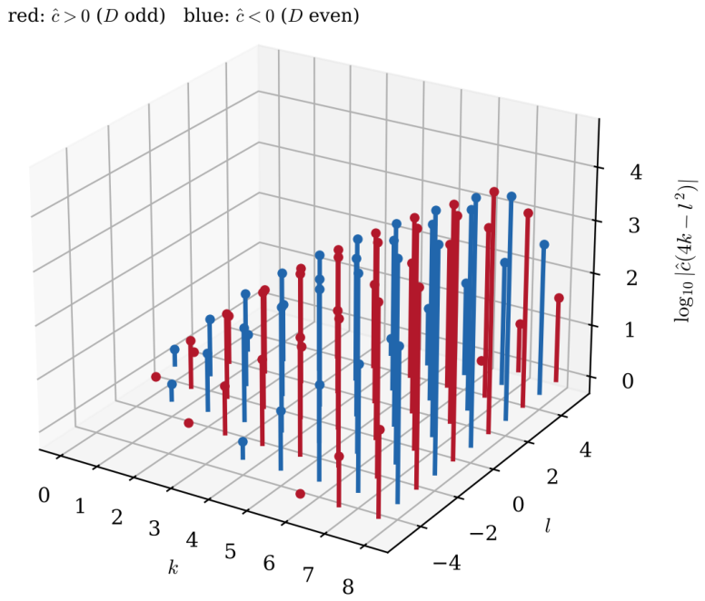
Figure 2.
From front to back: the upper bound of Lemma 5, the true values , the comparison series of Lemma 6, and its explicit lower bound , for . The lower bound grows like instead of ; Proposition 1 needs only that it beats the upper bound taken at a quarter of the argument.
Figure 2.
From front to back: the upper bound of Lemma 5, the true values , the comparison series of Lemma 6, and its explicit lower bound , for . The lower bound grows like instead of ; Proposition 1 needs only that it beats the upper bound taken at a quarter of the argument.
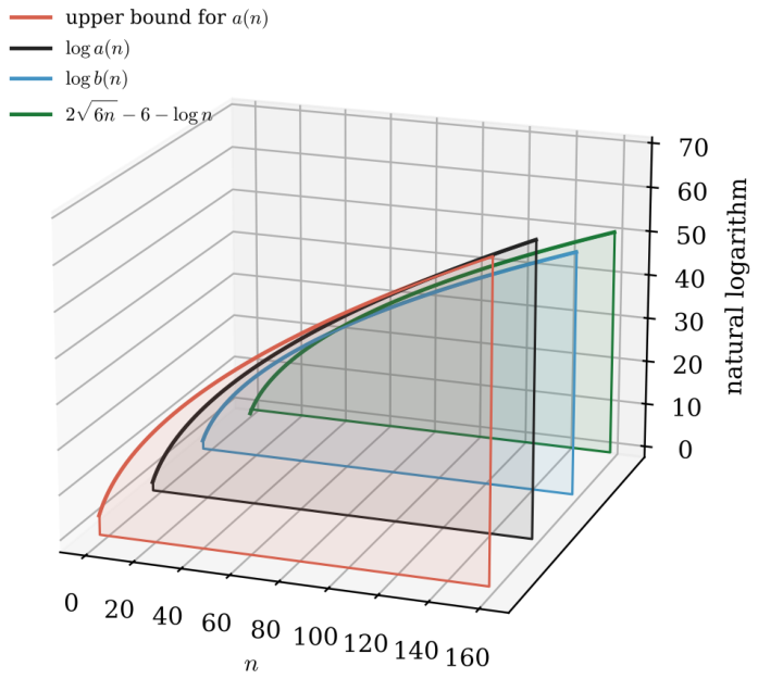
Figure 5.
The index for , and , on a logarithmic scale; the colour shows . The diagonal carries the largest and hence the most divisor terms, without visible effect on the size.
Figure 5.
The index for , and , on a logarithmic scale; the colour shows . The diagonal carries the largest and hence the most divisor terms, without visible effect on the size.
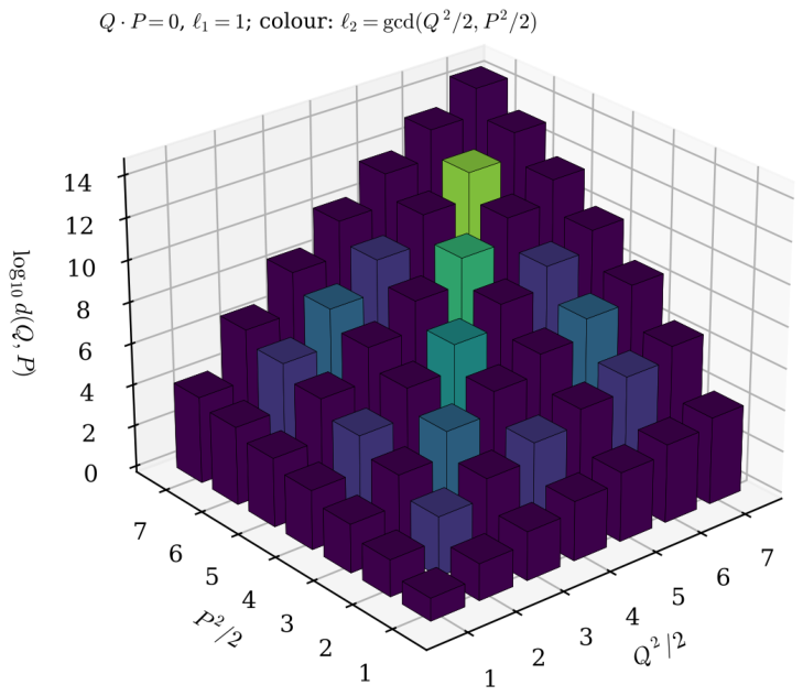
Figure 6.
The pairing in the proof of Theorem C for , , . The green points are paired with the red points ; the arrows carry the weights . The point lies at and carries the polar value ; against , where and , it attains the bound of Lemma 9.
Figure 6.
The pairing in the proof of Theorem C for , , . The green points are paired with the red points ; the arrows carry the weights . The point lies at and carries the polar value ; against , where and , it attains the bound of Lemma 9.
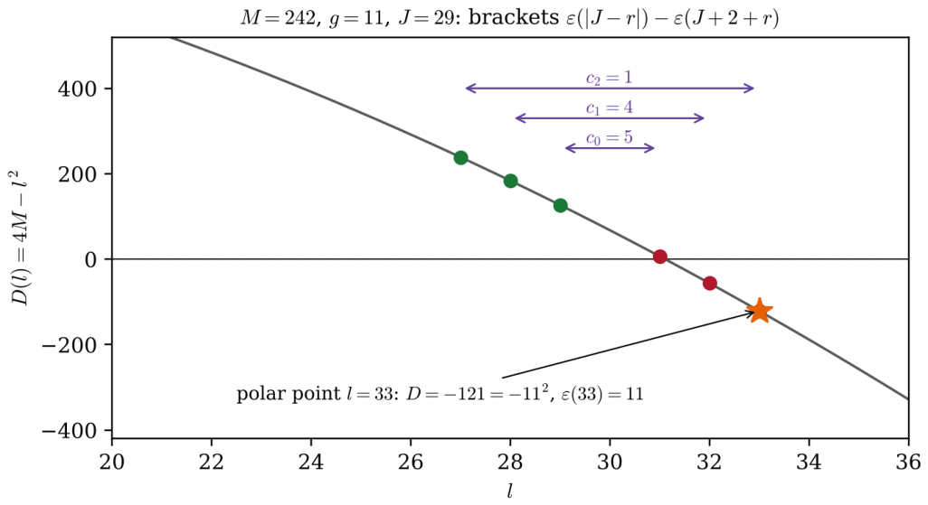
Figure 7.
The index at fixed angular momentum for , and all with , on a logarithmic scale.
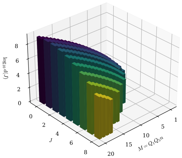
Table 1.
The index of (2) for small charges with . The column “terms” lists for the divisors of .
Table 1.
The index of (2) for small charges with . The column “terms” lists for the divisors of .
| terms | |||||||
|---|---|---|---|---|---|---|---|
| 1 | 1 | 0 | 1 | 1 | 4 | 12 | 12 |
| 1 | 1 | 1 | 1 | 1 | 3 | 8 | 8 |
| 2 | 1 | 1 | 1 | 1 | 7 | 39 | 39 |
| 2 | 2 | 0 | 1 | 2 | 16 | 684 | 708 |
| 2 | 2 | 1 | 1 | 1 | 15 | 513 | 513 |
| 2 | 2 | 2 | 1 | 2 | 12 | 208 | 192 |
| 3 | 3 | 3 | 1 | 3 | 27 | 11552 | 11576 |
| 2 | 4 | 2 | 1 | 2 | 28 | 14592 | 14514 |
| 4 | 4 | 4 | 1 | 4 | 48 | 928720 | 929104 |
| 4 | 4 | 0 | 1 | 4 | 64 | 15740076 | 15741492 |
| 6 | 6 | 6 | 1 | 6 | 108 | 10744220992 | 10744198464 |
| 4 | 1 | 2 | 2 | 1 | 12 | 208 | 192 |
| 9 | 1 | 3 | 3 | 1 | 27 | 11552 | 11576 |
| 4 | 3 | 2 | 2 | 1 | 44 | 431984 | 431680 |
| M | g | J | |||||
|---|---|---|---|---|---|---|---|
| 1 | 1 | 0 | 4 | 12 | 140 | 84 | |
| 1 | 1 | 1 | 3 | 8 | 112 | 96 | |
| 2 | 1 | 0 | 8 | 56 | 672 | 384 | |
| 2 | 1 | 1 | 7 | 39 | 546 | 453 | |
| 2 | 1 | 2 | 4 | 12 | 288 | 272 | |
| 3 | 1 | 0 | 12 | 208 | 2576 | 1392 | |
| 3 | 1 | 1 | 11 | 152 | 2128 | 1704 | |
| 3 | 1 | 2 | 8 | 56 | 1184 | 1096 | |
| 3 | 1 | 3 | 3 | 8 | 424 | 416 | |
| 4 | 2 | 0 | 16 | 708 | 8736 | 4662 | |
| 4 | 2 | 1 | 15 | 513 | 7230 | 5691 | |
| 4 | 2 | 2 | 12 | 192 | 4074 | 3690 | |
| 4 | 2 | 3 | 7 | 39 | 1539 | 1476 | |
| 9 | 3 | 0 | 36 | 85536 | 1138736 | 511664 | |
| 9 | 3 | 1 | 35 | 69168 | 982248 | 690992 | |
| 9 | 3 | 2 | 32 | 36088 | 627072 | 531872 | |
| 9 | 3 | 3 | 27 | 11576 | 291256 | 270608 | |
| 9 | 3 | 4 | 20 | 2032 | 95200 | 92512 | |
| 9 | 3 | 5 | 11 | 152 | 20648 | 20464 | |
| 8 | 2 | 0 | 32 | 36200 | 477420 | 220304 | |
| 8 | 2 | 1 | 31 | 28899 | 409531 | 293413 | |
| 8 | 2 | 2 | 28 | 14514 | 257116 | 220672 | |
| 8 | 2 | 3 | 23 | 4382 | 116118 | 108678 | |
| 8 | 2 | 4 | 16 | 708 | 36444 | 35592 | |
| 8 | 2 | 5 | 7 | 39 | 7440 | 7409 | |
| 16 | 4 | 0 | 64 | 15741492 | 216932868 | 85682720 | |
| 16 | 4 | 1 | 63 | 13311450 | 191469951 | 122262875 | |
| 16 | 4 | 2 | 60 | 7996158 | 131250148 | 103670560 | |
| 16 | 4 | 3 | 55 | 3339201 | 69207076 | 61136658 | |
| 16 | 4 | 4 | 48 | 929104 | 27579588 | 25923846 | |
| 16 | 4 | 5 | 39 | 159372 | 8070418 | 7849856 | |
| 16 | 4 | 6 | 28 | 14514 | 1655742 | 1639092 | |
| 16 | 4 | 7 | 15 | 513 | 220562 | 219993 | |
| 242 | 11 | 29 | 127 | 124029778470 | 19462192309545443 | 19462068157996872 | |
| 242 | 11 | 30 | 68 | 30442464 | 82875898355028 | 82875867912364 | |
| 242 | 11 | 31 | 7 | 39 | 124151548571 | 124151548466 |
Disclaimer/Publisher’s Note: The statements, opinions and data contained in all publications are solely those of the individual author(s) and contributor(s) and not of MDPI and/or the editor(s). MDPI and/or the editor(s) disclaim responsibility for any injury to people or property resulting from any ideas, methods, instructions or products referred to in the content. |
© 2026 by the authors. Licensee MDPI, Basel, Switzerland. This article is an open access article distributed under the terms and conditions of the Creative Commons Attribution (CC BY) license (http://creativecommons.org/licenses/by/4.0/).
Copyright: This open access article is published under a Creative Commons CC BY 4.0 license, which permit the free download, distribution, and reuse, provided that the author and preprint are cited in any reuse.