
Submitted:
08 November 2026
Posted:
11 November 2026
You are already at the latest version
Abstract
This study examines how real estate development shapes urban resilience under uncertainty, using a balanced panel of 21 prefecture-level cities in Guangdong, China, over 2005–2024. Real estate market development (REM) and urban resilience (UR) are measured with entropy-weighted composite indices, and their relationship is examined through coupling coordination analysis, two-way fixed-effects models, a moderating-effect model, a Hansen panel threshold model, and a spatial Durbin model. Four findings emerge. First, the coupling coordination degree rose from 0.233 in 2005 to a peak of 0.397 in 2019 and fell back to 0.280 in 2024, remaining within the imbalanced range throughout, with the Pearl River Delta (0.364) clearly leading the rest of the province. Second, real estate expansion exhibits a significant negative average association with urban resilience (−0.145, p < 0.05). Third, this association is state-dependent: the REM × UNC interaction is significantly positive (+2.130, p < 0.001), and the threshold test identifies an uncertainty threshold of 0.074 below which real estate development weakens resilience (−0.153) and above which it strengthens it (+0.752). Fourth, the spatial Durbin model reveals negative strategic interaction (ρ = −0.974) and a negative spillover from neighbouring real estate expansion (−0.471, p < 0.05), with the moderating mechanism concentrated in the Pearl River Delta. The results imply that the resilience function of the real estate market is a direction-switching function of the uncertainty environment, calling for state-contingent regulation, regionally coordinated governance, and a repositioning of real estate from a growth instrument toward a resilience support system.
Keywords:
real estate market
; urban resilience
; uncertainty
; coupling coordination
; spatial spillovers
; panel threshold model
1. Introduction
Cities in the contemporary world develop under conditions of heightened uncertainty. Slowing global growth, geopolitical tension, financial market volatility, public health emergencies, and extreme weather events interact and transmit into urban systems, so that urban development can no longer be assessed only by scale expansion and growth speed; it must also be assessed by the capacity of urban systems to resist, adapt to, recover from, and transform under shocks. This capacity—urban resilience—has become a central concept in urban research since Holling [1] first formalised resilience in ecological systems and Meerow et al. [2] defined urban resilience as the ability of urban systems and their social–ecological–technological networks to maintain, adapt, and transform under multi-scale shocks. The concept has since expanded from post-disaster recovery toward whole-process risk governance and long-term adaptive transformation [3,4].
Within urban systems, the real estate market occupies a special position. It concerns housing and quality of life, but it is also deeply embedded in local public finance, the banking system, the land system, infrastructure investment, and spatial governance. A moderately developed real estate market can enhance urban resilience through housing supply, infrastructure construction, urban renewal, and industrial linkages; excessive development can weaken it through housing price bubbles, crowding out of productive investment, financial fragility, and fiscal dependence on land conveyance. Housing market bubbles are not isolated price phenomena: they arise from the interaction of participants, expectations, and financial mechanisms and feed back into the stability of the urban system [5,6,7]. Whether real estate development supports or undermines urban resilience is therefore an empirical question rather than a matter of assumption.
Uncertainty deepens this already complex relationship. Economic policy uncertainty alters firm investment, household consumption, credit supply, and expectations [8], and recent Chinese evidence shows that the interaction between policy uncertainty and housing prices is time-varying rather than fixed in direction [9]. Because real estate is long-cycle, highly leveraged, and policy-sensitive, shifts in uncertainty should in principle change how real estate development affects urban systems. Yet most existing studies treat uncertainty either as a direct determinant of housing prices and investment or as a background variable, and rarely as a state variable that conditions the real estate–resilience relationship itself.
China provides an unusually clear setting in which to observe this conditioning role. Since the 1994 tax-sharing reform, land conveyance revenue has financed a substantial share of local infrastructure spending, so real estate has functioned as an instrument of urban growth rather than as a sector valued for its own output. The leverage rules introduced in 2020, followed by the liquidity distress of several large developers and the sharp contraction of presale volumes, converted a two-decade expansion into an abrupt adjustment within a few years. If the resilience contribution of the real estate market were fixed, this reversal should have produced a uniform deterioration of urban system performance; if it is state-dependent, the same contraction should have had different consequences in high- and low-uncertainty periods. Guangdong, where the adjustment began earliest and proceeded furthest, is therefore a particularly informative test case.
Against this background, this study examines the coupling between the real estate market and urban resilience in Guangdong Province, China, over 2005–2024. Guangdong is an instructive setting. It contains the Pearl River Delta (PRD), one of China’s most economically integrated urban agglomerations, alongside eastern, western, and northern regions with markedly weaker real estate demand and fiscal capacity, so the sample offers wide within-province variation in market conditions and resilience foundations. Four gaps in the literature motivate the analysis. First, real estate research has largely proceeded from prices, land finance, and investment, and has seldom evaluated the market’s consequences for urban system safety and adaptive capacity. Second, urban resilience research has only recently begun to incorporate real-estate-related variables, mainly through land marketisation [10], and has rarely treated the real estate market as a multidimensional subsystem of the urban system. Third, the conditional and nonlinear nature of the relationship—whether uncertainty switches its direction—has not been tested. Fourth, spatial interdependence between real estate markets and urban resilience within a single province has not been systematically examined.
This study makes three contributions. First, it places the real estate market and urban resilience in a common complex-systems framework in which both are treated as interacting adaptive subsystems rather than as independent outcome variables [11], and measures both with entropy-weighted composite indices covering six real estate dimensions and four resilience dimensions. Second, it identifies the conditions under which real estate development helps or harms resilience, using a moderating-effect model and a panel threshold model with the uncertainty state as the switching variable, thereby moving beyond the search for a single average effect. Third, it provides intra-provincial evidence on strategic spatial interaction, combining coupling coordination measurement with a spatial Durbin model that decomposes direct and spillover effects. The remainder of the paper reviews the literature and develops hypotheses, describes the data and methods, presents the results, and concludes with policy implications and limitations.
Three questions organise the analysis. First, does a coupling relationship exist between real estate market development and urban resilience, and how has its coordination level evolved across cities? Second, does the effect of real estate development on resilience change sign with the uncertainty environment, and if so, at what level of uncertainty does the switch occur? Third, does real estate development in one city impose costs on the resilience of its neighbours, converting what looks like a local growth strategy into an agglomeration-level problem? The first question is descriptive and is answered by coupling coordination measurement; the second and third are answered by conditional effect estimation and spatial decomposition.
2. Literature Review and Hypotheses
2.1. Urban Resilience and the Real Estate Market
The resilience concept originated in ecology, where Holling [1] defined it as the capacity of a system to absorb disturbance while maintaining structure and function, breaking with the single-equilibrium view of stability analysis. Meerow et al. [2] synthesised the urban literature and defined urban resilience as the ability of urban social–ecological–technological networks to persist, adapt, and transform under multi-scale shocks. Martin and Sunley [4] added an evolutionary perspective from regional economics: regional resilience is not merely the capacity to return to a pre-shock growth path but the capacity to adjust structure and create new development paths. Following these strands, urban resilience is understood here as a four-dimensional capacity—resistance, adaptation, recovery, and transformation—consistent with the multidimensional index constructions used in recent Chinese urban research [12,13].
Real estate fluctuations have long been analysed as cyclical phenomena with distinct phases of expansion, boom, adjustment, and recovery [14], embedded in a dynamic adjustment process between housing prices and supply [15]. Housing prices can deviate from fundamentals through money illusion and expectation dynamics [5,6], and land supply constraints combined with income agglomeration produce persistent price divergence across “superstar” cities [16]. The macroeconomic stakes of housing are well documented [17], as are the consequences of housing credit expansion [7]. Closest to this study, Chen et al. [10] show that land marketisation affects urban resilience in a large sample of Chinese cities, confirming that land and housing institutions belong inside the resilience question.
The four resilience dimensions are not equally exposed to real estate conditions, and specifying how each is exposed clarifies what the empirical tests should find. Resistance depends on the fiscal and institutional buffer available when a shock arrives; sustained land revenue can enlarge that buffer in the short run while making it pro-cyclical, because the same revenue collapses precisely when the shock hits. Adaptation depends on the capacity to reallocate factors and upgrade infrastructure; real estate expansion absorbs capital and labour that might otherwise flow into manufacturing upgrading and innovation, and it raises the cost of land for every other urban function. Recovery depends on the fiscal and household balance sheets that must finance post-shock repair; heavy mortgage commitments and developer leverage reduce the room to manoeuvre when incomes fall. Transformation depends on long-run investment in research, green infrastructure, and digital capacity, which competes with property for the same savings pool. The framework therefore predicts that crowding-out should be most visible in recovery, where balance-sheet constraints bind fastest, and least visible in transformation, where the relevant investments are slow-moving and partly financed from outside the city. Sect. 4.6 tests this prediction directly.
Three limitations of this literature frame the present analysis. First, the real estate market is usually reduced to one or two indicators, most often housing prices, whereas scale, supply, demand, financial linkage, and risk jointly characterise the market’s position within the urban system. Second, urban resilience studies rarely test the mechanisms through which real estate conditions feed into the four resilience dimensions. Third, coordination measurement and effect estimation are usually conflated: a high statistical association between two systems does not by itself imply benign coordination [18]. This study therefore separates the description of coordination states from the estimation of conditional effects.
2.2. Uncertainty as a Conditioning State
Knight [19] distinguished probabilisable risk from uncertainty that cannot be assigned probabilities. Risk governance scholarship reaches a parallel conclusion from the policy side: uncertainty is a property of the decision situation, not a measurement residual, and it has to be governed through institutional design rather than eliminated through better data [20]. Operationalising the latter, Baker et al. [8] constructed the economic policy uncertainty (EPU) index, which has become the standard proxy in studies of investment, credit, and asset prices. For China’s housing market, Chen et al. [21] built a real estate policy uncertainty index and linked it to declines in development investment and sales; Lu et al. [22] show that monetary policy uncertainty has time-varying effects on regional housing prices; Wang [23] finds that the spatial spillover identification of EPU on housing markets is sensitive to the uncertainty measure used; and Guan et al. [9] document two-way, time-varying causality between EPU and housing prices. EPU may also operate through local government debt and fiscal behaviour [24], a channel that is directly relevant to Chinese cities’ land finance dependence.
Two implications follow for the real estate–resilience nexus. First, the direction of the real estate effect should not be presumed: in normal periods, real estate expansion may crowd out productive investment and reinforce fiscal dependence, whereas in high-uncertainty periods, real estate serves as collateral and fiscal buffer, sustaining government spending capacity and financial stability. Second, because uncertainty in this operational sense is observable market volatility rather than deep uncertainty, it can be incorporated in panel models as both a moderating variable and a threshold variable [25].
The two mechanisms imply opposite signs and different time profiles, which is why an average effect estimated over a full cycle is not informative on its own. Crowding-out is gradual: it accumulates as land and credit are redirected, factor costs rise, and the local production structure narrows, so it should appear as a level effect in normal periods. Stabilisation is episodic: it operates through collateral values, the fiscal buffer, and the avoidance of fire sales during stress, so it should appear as a state-contingent shift rather than as a trend. A linear specification can only recover the average of the two, which is why the moderating and threshold models are estimated alongside the baseline rather than treated as robustness exercises. The distinguishing prediction is that the interaction between real estate development and uncertainty should be positive and large, and that the estimated marginal effect should cross zero within the observed range of the uncertainty index rather than outside it.
2.3. Coupling Coordination and Spatial Spillover Approaches
The coupling coordination degree model (CCDM) has been widely used to characterise the matching of urban subsystems, from environment–economy systems [18] to economic resilience and development quality in urban agglomerations [26]. Its advantage is descriptive: it distinguishes high-coupling-low-coordination states from benign high-level coordination, which simple correlation cannot do. Its limitation is equally clear: CCDM results cannot be interpreted as causal effects, which is why this study pairs it with econometric and spatial models.
Spatial dependence, in turn, is well established in regional data: ignoring it biases estimates [27,28]. Local clustering can be diagnosed with local indicators of spatial association (LISA) statistics [29], and spatial panel models allow the decomposition of direct and indirect effects [30]. Real estate markets are strongly spatial—prices, land supply, population flows, and developer behaviour are all linked across cities [16,31]—and urban resilience itself has spatial dimensions through infrastructure networks and industrial linkages. The spatial Durbin model (SDM) is therefore the natural vehicle for testing whether real estate expansion in one city affects resilience in neighbouring cities.
Combining the two approaches requires care about what each can deliver. Coupling coordination measurement establishes whether two subsystems are matched in level and whether the match is improving, but a high coordination degree is compatible with mutual deterioration, so it cannot support statements about effects. Spatial econometric estimation identifies conditional associations and their spatial decomposition, but it says nothing about the state of the system as a whole. Used together, the first describes where the real estate–resilience system sits and how it moved, and the second identifies which direction the relationship takes in different environments; neither substitutes for the other. The choice of weight matrix follows the same logic: an inverse-distance matrix truncated at 500 km represents the continuous reach of housing demand, commuting, and capital flows within a province better than a contiguity matrix, which in Guangdong would treat several non-neighbouring PRD cities as unrelated.
2.4. Hypotheses
The hypotheses below follow from the review and are ordered to match the empirical sequence in Sect. 3.5: H1 is examined by coupling coordination measurement, H2 and H3 by the fixed-effects and moderating models, H4 by the panel threshold model, H5 by the spatial Durbin model, and H6 by subsample and dimension-specific estimation. Each is stated so that it can fail.
H1.
A coupling relationship exists between the real estate market and urban resilience, and their coordination level exhibits temporal evolution and spatial differentiation.
H2.
Real estate market development has a dual effect on urban resilience: support within a reasonable development stage and harm under excessive expansion.
H3.
Uncertainty moderates the relationship between real estate development and urban resilience.
H4.
The effect of real estate development on urban resilience switches direction at an uncertainty threshold.
H5.
Real estate development in one city spills over to the urban resilience of neighbouring cities.
H6.
The relationship exhibits heterogeneity across regions and city sizes.
3. Data and Methods
3.1. Study Area and Data
The sample covers the 21 prefecture-level cities of Guangdong Province from 2005 to 2024, yielding 420 city-year observations. Nine PRD cities (Guangzhou, Shenzhen, Zhuhai, Foshan, Huizhou, Dongguan, Zhongshan, Jiangmen, Zhaoqing) are distinguished from four eastern (Shantou, Shanwei, Chaozhou, Jieyang), three western (Zhanjiang, Maoming, Yangjiang), and five northern (Shaoguan, Qingyuan, Meizhou, Heyuan, Yunfu) cities. All indicators are drawn from the Guangdong Statistical Yearbook, city-level statistical yearbooks, and the China City Statistical Yearbook, supplemented by the Peking University Digital Financial Inclusion Index. Missing values for early years are interpolated using city-level trend extrapolation with statistical-office consistency checks; outliers in growth rates attributable to statistical reclassification are winsorised at the 1st and 99th percentiles as a robustness step. Indicator selection was constrained by availability and statistical-calibre consistency, and the final systems below reflect the usable annual series.
Three features of the sample design deserve comment. First, the panel is balanced at 420 city-year observations: all 21 cities report every indicator in every year, so no observation is lost to attrition and the fixed-effects estimates are not affected by compositional change. Second, the sample deliberately covers the whole province rather than the PRD alone. Restricting attention to the nine PRD cities would maximise internal homogeneity but remove precisely the variation the analysis needs, because non-PRD cities differ from the PRD in real estate demand, fiscal capacity, and resilience foundations, and it is that contrast which identifies the regional heterogeneity reported in Sect. 4.6. Third, the start year is set by data comparability rather than by the real estate cycle: consistent city-level series on floor space sold, floor space under construction, and real estate lending are available from 2005 on a single statistical basis, while earlier yearbooks report them under definitions that cannot be reconciled without arbitrary adjustment.
3.2. Measuring the Real Estate Market
The real estate market development index (REM) aggregates eleven indicators in six dimensions—market scale, price level, supply capacity, demand base, financial linkage, and market risk—using the entropy weight method, which assigns weights according to the information content of each indicator [32] and avoids subjective weighting. Indicators expected to harm resilience when deviating from a desirable range (price-to-income ratio, inventory, volatility) are treated as negative or moderate attributes and standardised accordingly. Table 1 reports the system; in the estimated index, the housing investment share carries an entropy weight of 0.41 and the housing price level 0.26, with the remaining dimensions contributing the residual information.
The index is constructed in four steps. Indicators are first normalised to the unit interval, with positive attributes scaled by (x − min)/(max − min) and negative attributes by (max − x)/(max − min), so that a larger value always means a more developed market. Moderate attributes—those with a desirable interior range, such as the price-to-income ratio and the share of real estate in fixed-asset investment—are scaled by distance from a target value, so that deviation in either direction lowers the score. The information entropy of each indicator is then computed from its normalised distribution, with k = 1/lnn, and the weight is : the more evenly an indicator is distributed across observations, the less it discriminates and the smaller its weight. The composite index is the weighted sum of the normalised values. The outcome is that the two indicators with the strongest time-series discrimination—the housing investment share (0.41) and the housing price level (0.26)—carry most of the weight, while indicators that move almost uniformly across cities, such as the loan ratio, contribute little. This property matters for interpretation: REM is dominated by investment intensity and price level rather than by market scale in a simple sense, which is why single-indicator proxies fail to reproduce its coefficient in Sect. 4.6.
3.3. Measuring Urban Resilience
Urban resilience (UR) aggregates twelve indicators across the four dimensions of resistance, adaptation, recovery, and transformation (Table 2). The overall index is computed by placing all indicators in a single entropy-weighted system; hierarchical aggregation of the four dimensions and principal component analysis [33] are used as alternative constructions in robustness checks. The dimension indices are retained for the extended analysis of which resilience capacity is most affected by real estate conditions.
Two construction choices matter for interpretation. Placing all twelve indicators in a single entropy system lets the data determine the relative importance of the four dimensions, whereas equal weighting would impose the assumption that resistance and transformation count equally; both versions are estimated, with the single-system index reported as the main measure and equal weights, principal components, and a GDP-growth-stability proxy used as alternatives. The dimension indices are not used as separate dependent variables in the main models but only in the dimension-specific estimation of Sect. 4.6, where the question is which capacity absorbs the real estate effect. Because the four dimensions are correlated by construction, those coefficients are interpreted as indicating where the effect is concentrated rather than as independent structural parameters.
3.4. Measuring Uncertainty
Uncertainty (UNC) is operationalised as observable market-side volatility rather than deep uncertainty. The composite index combines housing price volatility (rolling standard deviation of residential price growth), real estate investment volatility (rolling standard deviation of investment growth), the national economic policy uncertainty index interacted with city real estate dependence, fiscal pressure (expenditure–revenue gap over revenue), and a dummy for the COVID-19 shock, aggregated by the entropy weight method (Table 3). This construction keeps the measure consistent across the 21 cities and 20 years, while remaining deliberately narrower than a complete measure of structural or geopolitical uncertainty.
A city-specific measure is preferred to the national policy uncertainty index alone for two reasons. The national index is common to all cities in a given year and is therefore absorbed by year fixed effects, so it cannot identify within-sample variation on its own; interacting it with city real estate dependence converts it into a city-year exposure measure that varies across space. The volatility components, by contrast, capture market-side uncertainty that is observable to households and developers at the local level, and fiscal pressure captures the resource constraint that determines how a city can respond to a shock. The composite thus combines external shock exposure, local market instability, and local fiscal capacity—the three channels through which uncertainty reaches the real estate–resilience relationship in the framework of Sect. 2.2.
Control variables are the logarithm of per capita GDP (lnPGDP), the tertiary industry share (IND), and the logarithm of resident population (lnPOP).
3.5. Empirical Strategy
The analysis proceeds in four steps. The first step measures coordination states. Following Liao [18], the coupling degree in Eq. (1) is
the comprehensive coordination index is Tit = 0.5 REMit + 0.5 URit, and the coupling coordination degree in Eq. (2) is
with D classified into six bands from severe imbalance (0–0.20) to high coordination (0.80–1.00). To identify which system lags, the relative development degree in Eq. (3) is
with R < 0.9 indicating a resilience-led state, 0.9 ≤ R ≤ 1.1 synchronised development, and R > 1.1 a market-led state. Coupling results are treated strictly as state measurement, never as causal evidence.
The second step estimates average and conditional effects with the two-way fixed-effects models of Eqs. (4) and (5):
where μi and λt are city and year fixed effects, standard errors are clustered at the city level, and UNC is centred in the interaction specification, so the marginal effect of REM is β1 + β3UNCit.
This marginal effect is reported at selected values of the uncertainty index rather than only at its mean, because the substantive question concerns how the effect changes across the uncertainty range; a single interaction coefficient states the sign of the change but not where the effect crosses zero. Because UNC is centred, β1 in Eq. (5) is the effect of REM at mean uncertainty, and the interaction is interpretable as the change in that effect per unit of uncertainty above or below the mean.
The third step tests regime switching with the Hansen [25] panel threshold model in Eq. (6):
The threshold is estimated by grid search over the interior of the UNC distribution, with the smallest and largest 5% of observations trimmed so that each regime retains enough observations for estimation; inference uses a bootstrap with 500 replications, and the null of linearity is tested against the single-threshold alternative. Only the single-threshold specification is reported, because with 420 observations a three-regime split would leave too few observations per regime to estimate the slope with useful precision, and because the economic question concerns the normal-versus-crisis distinction that one threshold already captures.
The fourth step addresses spatial dependence. Global Moran’s I [28] and LISA statistics [29] are computed for the levels, and Lagrange multiplier (LM) tests on the residuals guide model selection [27,30]. The spatial Durbin model in Eq. (7) is
with W a row-standardised inverse-distance matrix based on city coordinates, truncated at 500 km. Direct, indirect, and total effects are decomposed following Elhorst [30].
In matrix form the reduced form of Eq. (7) is UR = (I − ρW)−1(Xβ + WXθ)+…, so the effect of a change in a regressor is given by the partial derivatives of that inverse rather than by the coefficient alone. The average diagonal element of (I − ρW)−1(βkI + θkW) is the direct effect, the average row sum of its off-diagonal elements is the indirect effect, and the sum of the two is the total effect. Because the indirect effect depends on the entire weight matrix, it cannot be read off the coefficient on W ⋅ REM, and the two quantities are therefore reported separately. Heterogeneity is examined by subsample and interaction-term regressions across regions and city sizes, and the robustness battery replaces the core explanatory and dependent variables, lags REM, winsorises all continuous variables, excludes special cities, and runs a 500-draw placebo permutation test.
4. Results
4.1. Coordination Level and Temporal Evolution
The coupling coordination between the real estate market and urban resilience improved over the sample period but never escaped the imbalanced range (Figure 1). The annual mean of D rose from 0.233 in 2005 to 0.397 in 2019—the peak of the entire period—and fell back to 0.280 in 2024. The dynamics follow the real estate cycle closely. The annual mean of REM rose from 0.019 in 2005 to 0.134 in 2014, plunged to 0.066 in 2015 under inventory pressure, rose to 0.236 in 2018 and to 0.252 in 2019 during the shantytown redevelopment boom, and then declined to 0.059 in 2024. The annual mean of UR fell from 0.201 in 2005 to 0.086 in 2010, fluctuated between 0.09 and 0.19 thereafter (peaking at 0.181 in 2021), and stood at 0.131 in 2024. Coordination improvements driven by unilateral real estate expansion therefore lacked a resilience foundation and receded quickly in market downturns: the divergence between REM rising from 0.085 to 0.252 and UR rising only from 0.104 to 0.109 during 2017–2019 pushed D to its peak, which then collapsed as the market adjusted.
Four stage means summarise the trajectory: 0.301 in 2005–2008 (rapid expansion), 0.320 in 2009–2015 (intensified regulation), 0.340 in 2016–2020 (mounting uncertainty shocks), and 0.304 in 2021–2024 (structural adjustment). In the final stage the mean REM fell to 0.072 while mean UR remained at 0.149, above its second-stage level, indicating that the post-2021 decline in coordination was driven by real estate contraction rather than by degradation of resilience. Uncertainty amplified the swings: the composite UNC index never exceeded 0.008 before 2020 but jumped to 0.394 in 2020 and 0.392 in 2021, far above the threshold of 0.074 estimated below.
The grade distribution is highly concentrated. Moderately imbalanced cities account for 85.0% of all city-year observations, near coordination 11.2%, severe imbalance 1.9% (all in 2005, eight cities), and barely coordination 1.9% (scattered across 2006–2007 and 2020–2022). No city reached the moderate or high coordination grades; the highest value in the sample is 0.593, recorded in Guangzhou in 2021. Near-coordination cities were concentrated in 2018–2019—rising from one in 2017 to eight in 2018 and ten in 2019—and dwindled to one by 2022, showing that the upward window narrowed as the market receded.
4.2. Spatial Differentiation
Coordination levels are spatially stratified (Figure 2). Over 2005–2024, the mean D was 0.364 in the nine PRD cities, 0.266 in eastern, 0.284 in western, and 0.298 in northern Guangdong. The PRD is the only block above 0.30, confirming its lead, but the ranking of the other three blocks deviates from the usual expectation: eastern, not northern, Guangdong ranks lowest. All four blocks improved—the PRD from 0.294 (2005) to 0.329 (2024), eastern from 0.178 to 0.229, western from 0.196 to 0.241, and northern from 0.192 to 0.254, the largest gain (+0.062)—consistent with infrastructure catch-up and green transformation in the ecological-function-zone north. By 2024, however, all three non-PRD blocks remained within the 0.23–0.26 imbalance range.
The agglomeration gap is persistent. The mean D of the twelve non-PRD cities was 0.284 versus 0.364 for the PRD, a gap of 0.080 that widened in downturns: the two groups stood at 0.294 and 0.188 in 2005 (gap 0.105) and 0.409 and 0.282 in 2020 (gap 0.127), and both surged in 2019–2020 before the non-PRD group fell back faster after 2020 (Figure 3). Coordination outside the agglomeration thus lacks stable endogenous support, and the core–periphery gap tends to widen in market downturns rather than narrow.
City size produces a similar gradient. The mean D was 0.408 for the four large cities (Shenzhen, Guangzhou, Foshan, Dongguan), 0.314 for seven medium cities, and 0.285 for ten small-to-medium cities, with the ordering unchanged in 2024 (0.388, 0.269, 0.244). The relative development degree adds structure: market-led states (R > 1.1) account for 60.0% of large-city observations but only 27.1% and 6.5% of medium and small-to-medium observations, while resilience-led states (R < 0.9) account for 90.0% of small-to-medium observations. Large cities combine the highest coordination with the greatest risk of real estate outpacing resilience; small cities are dominated by the opposite imbalance, in which real estate development is insufficient to support resilience building.
4.3. Baseline and Moderating Effects
Table 4 reports the two-way fixed-effects estimates. In the baseline (M1), the coefficient on REM is −0.145 (clustered SE 0.063, p = 0.022, N = 420): after controlling for per capita GDP, industrial structure, and population, real estate expansion is associated with significantly lower urban resilience. The controls behave as expected—lnPGDP (0.080, p = 0.014), IND (0.106, p < 0.001), and lnPOP (0.106, p = 0.030) are all positive—indicating that economic development, the service economy, and population agglomeration remain the fundamental supports of resilience. Adding UNC (M2) narrows the REM coefficient to −0.118 (p = 0.032) while UNC itself enters at +0.452 (SE 0.058, p < 0.001): uncertainty periods are associated with higher measured resilience, consistent with the intensification of resilience investment during crises.
The moderating effect is strong. The REM × UNC interaction is +2.130 (SE 0.588, p = 0.0003, M3), significantly positive at the 1% level: the higher the uncertainty, the smaller the resilience cost of real estate development, up to a reversal. The economic logic is that when shocks weigh on activity, real estate serves as the core collateral and fiscal buffer, sustaining government spending capacity and financial stability, and thereby partially offsetting its crowding-out effect in normal times. A quadratic REM term added to M1 is insignificant and leaves the linear estimate essentially unchanged, so the nonlinearity in the relationship arises from state switching in the uncertainty environment rather than from market scale itself. These results support H3.
The interaction can be read concretely by evaluating the marginal effect at points of the observed uncertainty distribution. At zero uncertainty the model implies a marginal effect of −0.038, at the estimated threshold of 0.074 it implies +0.119, and at the 2020–2021 level of about 0.39 it implies +0.80. Two features of this profile matter. First, the implied zero crossing in the linear interaction model (0.018) lies well below the threshold estimate of 0.074, which means the switch is not a smooth rotation of the slope: the data are better described by a discrete regime change, and the linear interaction overstates the effect at moderate uncertainty while understating it in extreme episodes. Second, the coefficient on REM alone in M3 (−0.038) is no longer significant, which is not evidence that real estate development is harmless—it is the effect at mean uncertainty only, while the pooled coefficient in M1 remains the relevant average over the sample.
The magnitude is best judged against the observed variation. Across the sample REM has a standard deviation of 0.086 and UR of 0.062, so the baseline coefficient of −0.145 implies that a one-standard-deviation increase in real estate development is associated with a fall of about 0.012 in the resilience index, roughly one-fifth of a standard deviation of UR. The association is strongest in the stage in which real estate expanded fastest: 2017–2019, when mean REM rose from 0.085 to 0.252 while mean UR moved only from 0.104 to 0.109, is the clearest instance of divergence between the two systems.
The controls also carry information about the composition of resilience. The positive and significant coefficient on the tertiary share indicates that service-sector depth supports resilience independently of real estate, and its stability across specifications (0.094 to 0.106) suggests that the real estate effect is not proxying for industrial structure. Population is significant in M1 and M2 but loses significance once the interaction is included, consistent with the reading that population growth and real estate expansion are correlated channels of the same urban growth process rather than independent supports.
4.4. Threshold Effect
The Hansen test confirms the regime structure (Table 5). The single-threshold specification yields an F statistic of 6.52 with a bootstrap p-value below 0.01 and a threshold estimate of UNC* = 0.074. Below the threshold, the REM coefficient is −0.153 (p = 0.017), consistent with the baseline; above it, the coefficient turns to +0.752 (p = 0.0001). The threshold lies in the upper-middle range of the sample uncertainty distribution and corresponds to high-volatility episodes such as the 2020 pandemic shock and the 2016–2017 regulatory tightening. Suppression in normal times and support in crises are thus captured as a parameter switch in the same specification rather than as two separate models, and the two coexisting mechanisms—crowding-out and stabilisation—are both identified in the data. H4 is supported.
The two regime coefficients differ by 0.905, an order of magnitude larger than the standard error of either, so the regime distinction is not a marginal refinement of the baseline estimate. The threshold value is itself economically interpretable: 0.074 lies between the near-zero uncertainty of 2005–2019, when the composite index rarely exceeded 0.01, and the extreme values of 2020–2021, which reached about 0.39. In practice the estimate therefore separates ordinary years from crisis years rather than dividing the normal period into two regimes, and the low-uncertainty coefficient of −0.153 should be read as the effect that prevailed for most of the sample.
This also explains why the average effect is negative. Because the large majority of observations fall below the threshold, the pooled coefficient in M1 is dominated by the low-uncertainty regime and is close to the regime-specific estimate (−0.145 versus −0.153). Crises are too rare in a 20-year panel to move the average, but they are frequent enough, and the coefficient large enough, to matter for policy: the support effect of +0.752 is roughly five times the magnitude of the suppression effect in normal times, so a short crisis episode can offset several years of crowding-out in cumulative terms.
4.5. Spatial Spillovers
Zero-order global Moran’s I statistics for the UR and REM levels are weak and insignificant, which is not unusual for a single-province sample in which intra-agglomeration competition dominates, and does not preclude conditional spatial dependence. Residual diagnostics provide the sharper evidence: LM-lag = 12.91 (p = 0.0003), robust LM-lag = 4.72 (p = 0.030), and LM-error = 11.93 (p = 0.0006), all justifying a spatial specification. The SDM estimates (Table 6) show a significantly negative spatial autoregressive coefficient (ρ = −0.974, SE 0.250, p = 0.0001), indicating strategic divergence rather than convergence in resilience performance, and a significantly negative spatial lag of REM (W·REM = −0.471, SE 0.229, p = 0.040): real estate expansion in neighbouring cities exerts negative pressure on local resilience, consistent with a siphon-and-competition mechanism in which investment and population are drawn away.
Effect decomposition shows a direct effect of −0.131, an indirect effect of +0.068, and a total effect of −0.063: the resilience cost of local real estate development is borne primarily by the developing city itself, while neighbours obtain partially compensatory gains through factor reflux. Given that ρ is close to the parameter boundary, its magnitude should not be read as an elasticity; the robust content of the result is the negative direction of strategic interaction and the significant negative neighbour spillover. H5 is supported.
The direct and indirect effects point in opposite directions, which explains why the total effect is small (−0.063) despite a substantial direct effect (−0.131). A city that expands its real estate sector bears a resilience cost itself, but part of that cost is offset by gains accruing to it from neighbours’ expansion, so the net provincial effect understates the local one. This asymmetry has a direct governance implication: from an individual city’s perspective, restraint is costly and confers benefits that are partly captured elsewhere, which is the structure of a collective action problem rather than of a simple externality.
The negative spatial autoregressive coefficient deserves separate comment. A value of −0.974 implies that a positive shock to one city’s resilience is associated with lower resilience in its neighbours once the covariates are controlled. Read as strategic interaction, this is a competition effect: cities in the same agglomeration compete for the mobile factors—investment, skilled labour, headquarters functions—that underpin resilience, and improvement in one is partly achieved at the expense of another. Read as a mechanical property of the weight matrix it is less informative, which is why the sign rather than the magnitude is the robust content of the estimate. Either reading is inconsistent with the assumption that resilience improvements diffuse automatically across space.
4.6. Heterogeneity and Robustness
Regional heterogeneity operates through the moderating channel rather than through average levels. Subsample baseline coefficients are insignificant in both groups—−0.023 (p = 0.772) in the PRD and 0.001 (p = 0.986) in the non-PRD—while the REM × UNC interaction is significant in the PRD (+1.913, SE 0.899, p = 0.035) but not in the non-PRD (+3.009, p = 0.308, wide standard error). The state-switching mechanism is thus concentrated where the financial system is well developed and factor mobility is frequent. City-size grouped regressions suffer from small within-group samples and are not treated as primary evidence. Across resilience dimensions (Figure 4), the resilience cost of real estate expansion is concentrated in recoverability (−0.352, SE 0.216, p = 0.104), the largest estimate in absolute value, while resistance (−0.064, p = 0.559), adaptation (−0.018, p = 0.531), and transformation (+0.010, p = 0.943) show no significant effects. The crowding-out operates mainly on post-shock recovery capacity—fiscal, consumption, and employment recovery—rather than on infrastructure carrying capacity or long-term transformation.
The conclusions survive a battery of checks (Table 7). Single-dimension proxies for REM produce insignificant coefficients—investment intensity (0.003, p = 0.986), per-capita floor space sold (0.005, p = 0.552), housing affordability (−0.007, p = 0.506), and inverse price volatility (0.036, p = 0.127)—showing that the composite index, in which the housing investment share (entropy weight 0.41) and price level (0.26) dominate, carries information that no single dimension reproduces; none of the proxies supports the alternative conclusion that real estate promotes resilience. Alternative UR constructions preserve the direction: equal weights (−0.085, p = 0.107), PCA (−0.107, p = 0.233), and a GDP-growth-stability proxy (−0.036, p = 0.243). The one-period-lagged REM coefficient is −0.110 (p = 0.139), indicating persistence with attenuation. Winsorisation strengthens the result (−0.208, p = 0.017). Excluding Guangzhou and Shenzhen (−0.122, p = 0.087), Guangzhou only (−0.153, p = 0.045), resource-based cities (−0.139, p = 0.029), or the population-growth extremes (−0.128, p = 0.030) leaves the coefficient negative in all four cases. In the placebo test, 500 random permutations of REM across observations yield a mean spurious coefficient of −0.0002 with a standard deviation of 0.025; none of the draws reaches the absolute value of the true coefficient, and 5.6% are spuriously “significant,” close to the nominal rate.
Taken together, H1, H3, H4, and H5 are supported; H6 receives conditional support at the moderating level; and H2 is partially supported—the claim that excessive expansion harms resilience is consistent with the negative baseline and threshold results, while no evidence emerges that real estate development at a “reasonable stage” promotes resilience on average.
5. Discussion
The central finding is that the resilience function of the real estate market is a direction-switching function of the uncertainty environment rather than a fixed parameter. In normal periods, real estate expansion crowds out resilience: land and credit concentrate in real estate, factor costs rise, and fiscal dependence on land conveyance deepens, eroding the capacity to withstand shocks. In high-uncertainty periods, the same expansion hedges: real estate sustains collateral values, fiscal spending capacity, and financial stability precisely when other channels contract. This reading is consistent with the literature on policy uncertainty and housing markets, in which the safe-haven and collateral functions of housing become more prominent as uncertainty rises [8,9], and it extends that literature to the resilience dimension, which prior Chinese studies have approached mainly through land marketisation [10] or through resilience measurement alone [12,13].
Three implications follow for how the real estate–resilience relationship should be theorised. First, the relationship is state-contingent rather than a level relationship, and the conditioning variable is the uncertainty environment rather than the stage of development or the size of the sector. Specifications that search for a single elasticity, or that test for a quadratic in market scale, are therefore likely to return weak or unstable estimates: in this sample a quadratic term adds nothing, while a regime split produces coefficients that differ by a factor of five. Second, the direction of the effect is not a property of real estate as such but of what the sector is doing in the urban economy. Where real estate functions as a growth instrument—financing infrastructure through land revenue and absorbing savings that might otherwise fund productive upgrading—expansion crowds out resilience; where it functions as a collateral and fiscal buffer, the same expansion supports it. The policy question is consequently not how much real estate a city should have but which function the sector is performing. Third, the spatial results imply that the relevant unit of analysis is the agglomeration rather than the city, because the resilience cost of expansion is partly exported and the benefit of restraint partly imported.
These findings also qualify the existing Chinese evidence in two ways. Studies that treat land marketisation as the institutional channel [10] identify an effect running through the supply side and the fiscal system; the results here suggest that the sign of that effect depends on the uncertainty environment, which those designs do not model and which may explain variation in reported estimates across samples and periods. Studies that measure resilience without modelling its real estate determinants [12,13] supply the outcome variable but not the mechanism; the dimension-specific results indicate that the mechanism operates mainly through recovery capacity, which is consistent with a balance-sheet channel rather than an infrastructure channel. Both strands are compatible with the state-switching account developed here, and neither is sufficient without it.
The coordination results qualify the econometric findings. Coordination improvements during 2005–2019 were driven by unilateral real estate expansion without matching resilience accumulation, and they receded as soon as the market adjusted; only eight city-years—1.9% of the sample, all of them in Guangzhou and Shenzhen—crossed the barely-coordinated boundary, none of them durably, and the PRD’s advantage widened in downturns. Coupling measurement and effect estimation therefore tell one coherent story from two angles: the state-level pattern (a leading PRD, a catching-up periphery) and the effect-level pattern (crowding-out in normal times, hedging in crises, negative spatial competition) both describe a system in which real estate has been a growth instrument rather than a resilience support.
Three caveats bound the interpretation. First, the analysis identifies robust conditional correlations, not causal effects: reverse causality—resilient cities attracting more real estate development—would bias the baseline coefficient toward positive, so the negative estimate is best read as a conservative lower bound, and no quasi-experimental identification strategy is claimed. Second, the uncertainty measure is deliberately narrow: it proxies observable market volatility and shock exposure, not deep structural uncertainty, and the EPU interaction is a macro exposure proxy rather than a city-specific uncertainty measure. Third, the spatial autoregressive estimate lies near the parameter boundary; its magnitude should not be interpreted as an elasticity, and the spillover decomposition should be read directionally. The negative association is also insensitive to the weighting scheme, the index construction, and sample composition, which strengthens confidence in the sign but not in the precision of magnitudes.
6. Conclusions and Policy Implications
This study examined the coupling between real estate development and urban resilience in 21 Guangdong cities over 2005–2024 using coupling coordination analysis, fixed-effects and threshold models, and a spatial Durbin model. Three conclusions follow. First, coordination between the real estate market and urban resilience improved over two decades but remained within the imbalanced range, with a persistent PRD lead and barely-coordinated status confined to eight isolated city-years in Guangzhou and Shenzhen. Second, real estate expansion has, on average, a significant negative association with urban resilience that is concentrated in the recovery dimension and reverses under high uncertainty: the estimated threshold of 0.074 separates a low-uncertainty regime of suppression (−0.153) from a high-uncertainty regime of support (+0.752). Third, spatial interaction is strategically competitive: neighbouring real estate expansion reduces local resilience, local crowding-out dominates the total effect, and the moderating mechanism is concentrated in the PRD.
Two qualifications should travel with these conclusions. The state-switching mechanism is identified with an uncertainty measure that is observable and market-based, not with deep uncertainty; a broader measure incorporating geopolitical or structural risk might locate the threshold differently, and the estimated value of 0.074 should be treated as sample-specific rather than as a policy target. And the spatial estimates describe strategic interaction within a single province, where the competitors share one administrative and fiscal system; in cross-province settings the form of competition may differ, and the negative interaction need not carry over with the same sign.
The policy implications follow from the state-contingent structure of the findings. First, real estate policy should be repositioned from a growth instrument toward a resilience support system: objectives should extend from stabilising investment, sales, and prices to stabilising housing, risk, space, and resilience, with supply grounded in genuine demand, development steered toward urban renewal and inefficient-land redevelopment, and the residential attribute reinforced. Second, regulation should be state-contingent: deleveraging and dependence reduction should be pursued resolutely in low-uncertainty periods, while moderate continuity of real estate financing should be maintained in high-uncertainty periods, because one-size-fits-all contraction in crisis periods amplifies systemic risk. Third, a joint monitoring system should track housing affordability, real estate financial risk, land finance risk, supply–demand matching, and urban resilience together, since the threshold result implies that risk accumulates gradually before switching regimes. Fourth, governance should be regionally coordinated: the negative neighbour spillover implies that uncoordinated expansion within agglomerations shifts rather than solves the problem, calling for metropolitan-level coordination of housing supply, transportation, public services, and real estate risk prevention. Fifth, policy should be differentiated by city type: large cities require risk prevention and quality improvement given their market-led imbalance; medium cities require supply optimisation; small and outflow cities require inventory control and industrial transformation rather than further real estate expansion.
The study has limitations that define the research agenda. The indicator systems are constrained by city-level data availability—vacancy rates, household leverage, and developer debt risk cannot yet be incorporated; the uncertainty measure could be enriched with city-specific financial and fiscal volatility; causal identification requires quasi-experimental designs exploiting regulatory shocks; and the spatial weight matrix could be replaced with networks built from population migration, commuting, and corporate investment data. Extending the analysis to micro-level data and to cross-province or cross-country samples would allow the external validity of the state-switching mechanism documented here to be tested.
Funding
This research received no external funding.
Competing: Interests
The authors declare that they have no known competing financial interests or personal relationships that could have appeared to influence the work reported in this paper.
Ethics Approval
Not applicable. This study uses only aggregated, publicly available statistical data at the city level; no human participants or animals are involved, and no individual-level or identifiable information is used.
Consent to Participate and Consent for Publication
Not applicable for the reasons given above.
Data Availability All Data Are Drawn from Publicly Available Sources
the Guangdong Statistical Yearbook, city-level statistical yearbooks, the China City Statistical Yearbook, and the Peking University Digital Financial Inclusion Index. The derived panel dataset is available from the corresponding author on reasonable request.
Use of Generative Artificial Intelligence a Large Language Model-Based Writing Assistant Was Used for Three Purposes
translating and refining the language of an earlier Chinese-language draft of this paper; suggesting structural and stylistic improvements to individual passages; and checking the formatting and internal consistency of the reference list. The tool was not used to generate the research questions, hypotheses, empirical strategy, results, or conclusions, all of which derive from the authors’ own analysis of the data. The authors verified every suggested change against the underlying data and the cited sources, and take full responsibility for the content of the manuscript.
References
- Holling, C.S. Resilience and Stability of Ecological Systems. Annu. Rev. Ecol. Syst. 1973, 4, 1–23. [Google Scholar] [CrossRef]
- Meerow, S.; Newell, J.P.; Stults, M. Defining Urban Resilience: A Review. Landsc. Urban Plan. 2016, 147, 38–49. [Google Scholar] [CrossRef]
- Cutter, S.L.; Barnes, L.; Berry, M.; Burton, C.; Evans, E.; Tate, E.; Webb, J. A Place-Based Model for Understanding Community Resilience to Natural Disasters. Glob. Environ. Change 2008, 18, 598–606. [Google Scholar] [CrossRef]
- Martin, R.; Sunley, P. On the Notion of Regional Economic Resilience: Conceptualization and Explanation. J. Econ. Geogr. 2015, 15, 1–42. [Google Scholar] [CrossRef]
- Case, K.E.; Shiller, R.J. Is There a Bubble in the Housing Market? Brook. Pap. Econ. Act. 2003, 2003, 299–362. [Google Scholar] [CrossRef]
- Brunnermeier, M.K.; Julliard, C. Money Illusion and Housing Frenzy. Rev. Financ. Stud. 2008, 21, 135–180. [Google Scholar] [CrossRef]
- Mian, A.; Sufi, A. The Consequences of Mortgage Credit Expansion: Evidence from the U.S. Mortgage Default Crisis. Q. J. Econ. 2009, 124, 1449–1496. [Google Scholar] [CrossRef]
- Baker, S.R.; Bloom, N.; Davis, S.J. Measuring Economic Policy Uncertainty. Q. J. Econ. 2016, 131, 1593–1636. [Google Scholar] [CrossRef]
- Guan, Y.; Wang, Y.; Su, C. The Two-Way Impact between Economic Policy Uncertainty and Housing Prices in China: Sub-Sample Time-Varying Causality Analysis. Buildings 2025, 15, 1550. [Google Scholar] [CrossRef]
- Chen, M.; Zeng, L.; Deng, Y.; Chen, S.; Gu, X. The Impact of Land Marketization on Urban Resilience: Empirical Evidence from Chinese Cities. Land 2024, 13, 1385. [Google Scholar] [CrossRef]
- Holland, J.H. Studying Complex Adaptive Systems. J. Syst. Sci. Complex. 2006, 19, 1–8. [Google Scholar] [CrossRef]
- Yao, F.; Li, L.; Liang, J. Spatial and Temporal Evolution of Urban Resilience in China and Analysis of Barriers: Based on a Sustainable Development Perspective. PLoS ONE 2024, 19, e0285113. [Google Scholar] [CrossRef]
- Shi, H.; Hu, Y.; Gan, L. Assessing Urban Resilience Based on Production–Living–Ecological System Using Degree of Coupling Coordination: A Case of Sichuan. PLoS ONE 2024, 19, e0304002. [Google Scholar] [CrossRef]
- Pyhrr, S.A.; Roulac, S.E.; Born, W.L. Real Estate Cycles and Their Strategic Implications for Investors and Portfolio Managers in the Global Economy. J. Real. Estate Res. 1999, 18, 7–68. [Google Scholar] [CrossRef]
- DiPasquale, D.; Wheaton, W.C. The Markets for Real Estate Assets and Space: A Conceptual Framework. Real. Estate Econ. 1992, 20, 181–198. [Google Scholar] [CrossRef]
- Gyourko, J.; Mayer, C.; Sinai, T. Superstar Cities. Am. Econ. J. Econ. Policy 2013, 5, 167–199. [Google Scholar] [CrossRef]
- Muellbauer, J.; Murphy, A. Housing Markets and the Economy: The Assessment. Oxf. Rev. Econ. Policy 2008, 24, 1–33. [Google Scholar] [CrossRef]
- Liao, C. Quantitative Judgement and Classification System for Coordinated Development of Environment and Economy: A Case Study of the Urban Agglomeration in the Pearl River Delta. Trop. Geogr. (in Chinese). 1999, 19, 171–177. [Google Scholar] [CrossRef]
- Knight, F.H. Risk, Uncertainty and Profit; Houghton Mifflin: Boston, MA, USA, 1921. [Google Scholar]
- Renn, O. Risk Governance: Coping with Uncertainty in a Complex World; Earthscan: London, UK, 2008. [Google Scholar] [CrossRef]
- Chen, Y.; Mo, D.; Tang, S.; Li, H. Measuring Real Estate Policy Uncertainty in China. China Econ. Q. (in Chinese). 2022, 22, 405–424. [Google Scholar] [CrossRef]
- Lu, Y.; Li, J.; Yang, H. Time-Varying Impacts of Monetary Policy Uncertainty on China’s Housing Market. Econ. Model. 2023, 118, 106081. [Google Scholar] [CrossRef]
- Wang, X. Unveiling the Multiscale Impact of Economic Policy Uncertainty on China’s Housing Market Spillovers: Evidence from Different Uncertainty Measurements. Financ. Res. Lett. 2023, 58, 104603. [Google Scholar] [CrossRef]
- Gao, H.; Lan, M.; Li, J.; Zhou, T. Economic Policy Uncertainty and Local Government Debt: Evidence from China. Kyklos 2024, 77, 1103–1141. [Google Scholar] [CrossRef]
- Hansen, B.E. Threshold Effects in Non-Dynamic Panels: Estimation, Testing, and Inference. J. Econom. 1999, 93, 345–368. [Google Scholar] [CrossRef]
- Ma, S.; Huang, J. Analysis of the Spatio-Temporal Coupling Coordination Mechanism Supporting Economic Resilience and High-Quality Economic Development in the Urban Agglomeration in the Middle Reaches of the Yangtze River. PLoS ONE 2023, 18, e0281643. [Google Scholar] [CrossRef]
- Anselin, L. Spatial Econometrics: Methods and Models; Kluwer Academic Publishers: Dordrecht, The Netherlands, 1988. [Google Scholar] [CrossRef]
- Moran, P.A.P. Notes on Continuous Stochastic Phenomena. Biometrika 1950, 37, 17–23. [Google Scholar] [CrossRef]
- Anselin, L. Local Indicators of Spatial Association—LISA. Geogr. Anal. 1995, 27, 93–115. [Google Scholar] [CrossRef]
- Elhorst, J.P. Spatial Econometrics: From Cross-Sectional Data to Spatial Panels; Springer: Berlin/Heidelberg, Germany, 2014. [Google Scholar] [CrossRef]
- Krugman, P. Increasing Returns and Economic Geography. J. Political Econ. 1991, 99, 483–499. [Google Scholar] [CrossRef]
- Shannon, C.E. A Mathematical Theory of Communication. Bell Syst. Tech. J. 1948, 27, 379–423. [Google Scholar] [CrossRef]
- Pearson, K. On Lines and Planes of Closest Fit to Systems of Points in Space. Lond. Edinb. Dublin Philos. Mag. J. Sci. 1901, 2, 559–572. [Google Scholar] [CrossRef]
Figure 1.
Temporal evolution of the coupling coordination degree (annual mean, 2005–2024). Dashed lines mark the near-coordination (0.40) and barely-coordinated (0.50) boundaries.
Figure 1.
Temporal evolution of the coupling coordination degree (annual mean, 2005–2024). Dashed lines mark the near-coordination (0.40) and barely-coordinated (0.50) boundaries.
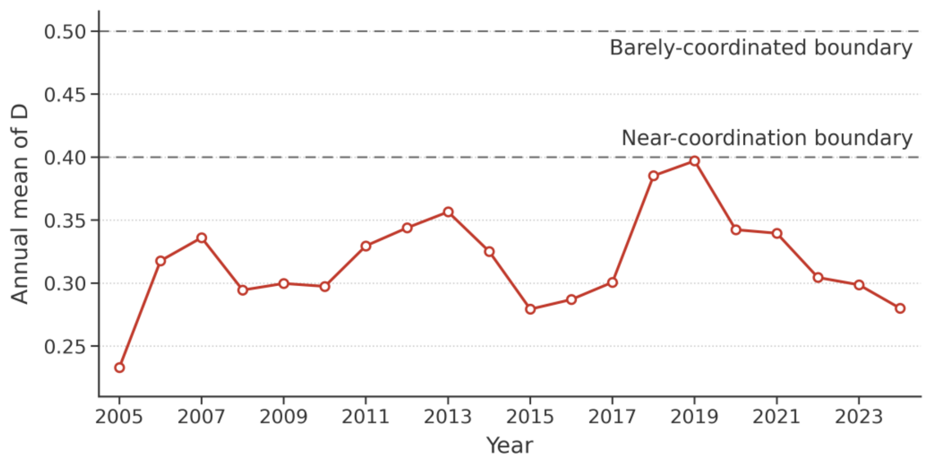
Figure 2.
Spatial distribution of the coupling coordination degree by city and year, 2005–2024.
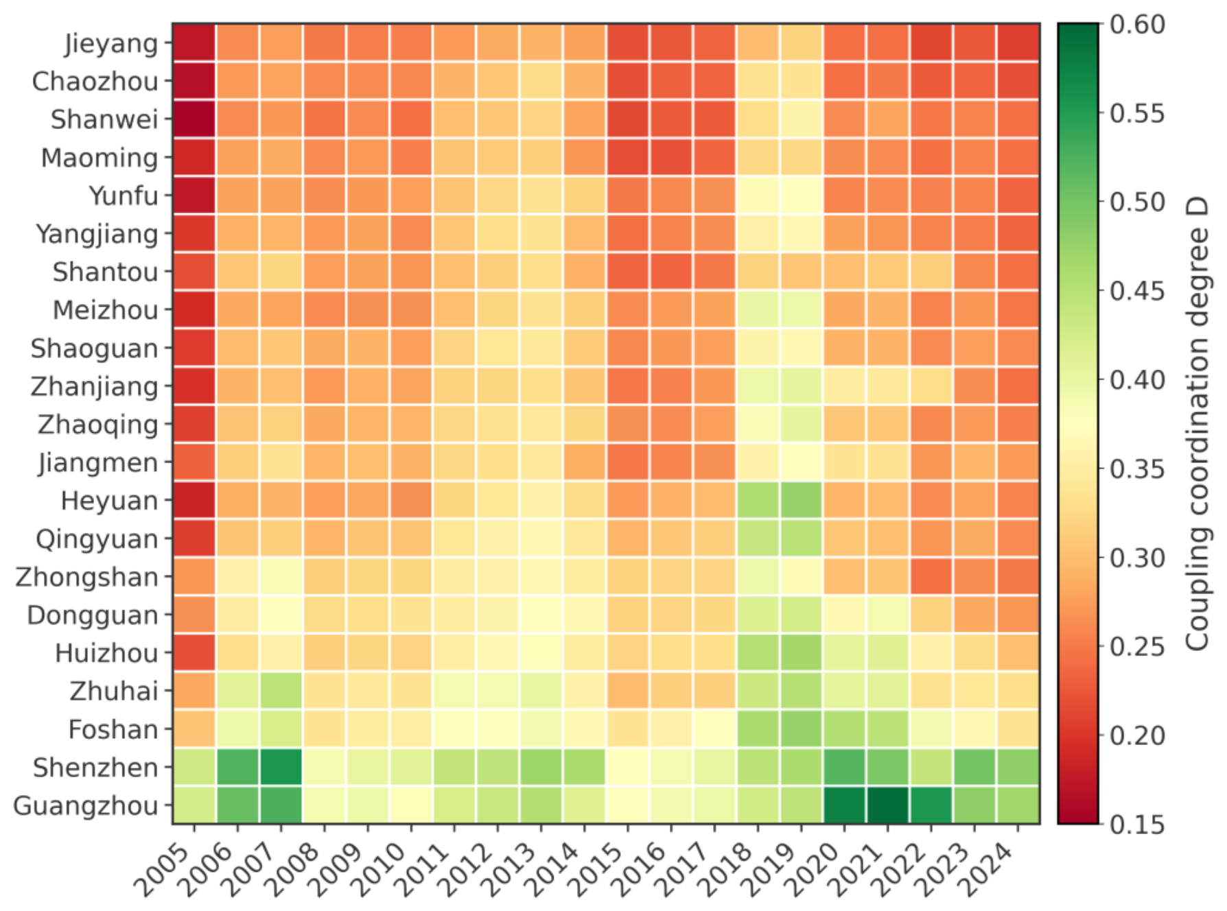
Figure 3.
Coupling coordination degree: nine PRD cities versus twelve non-PRD cities, 2005–2024.
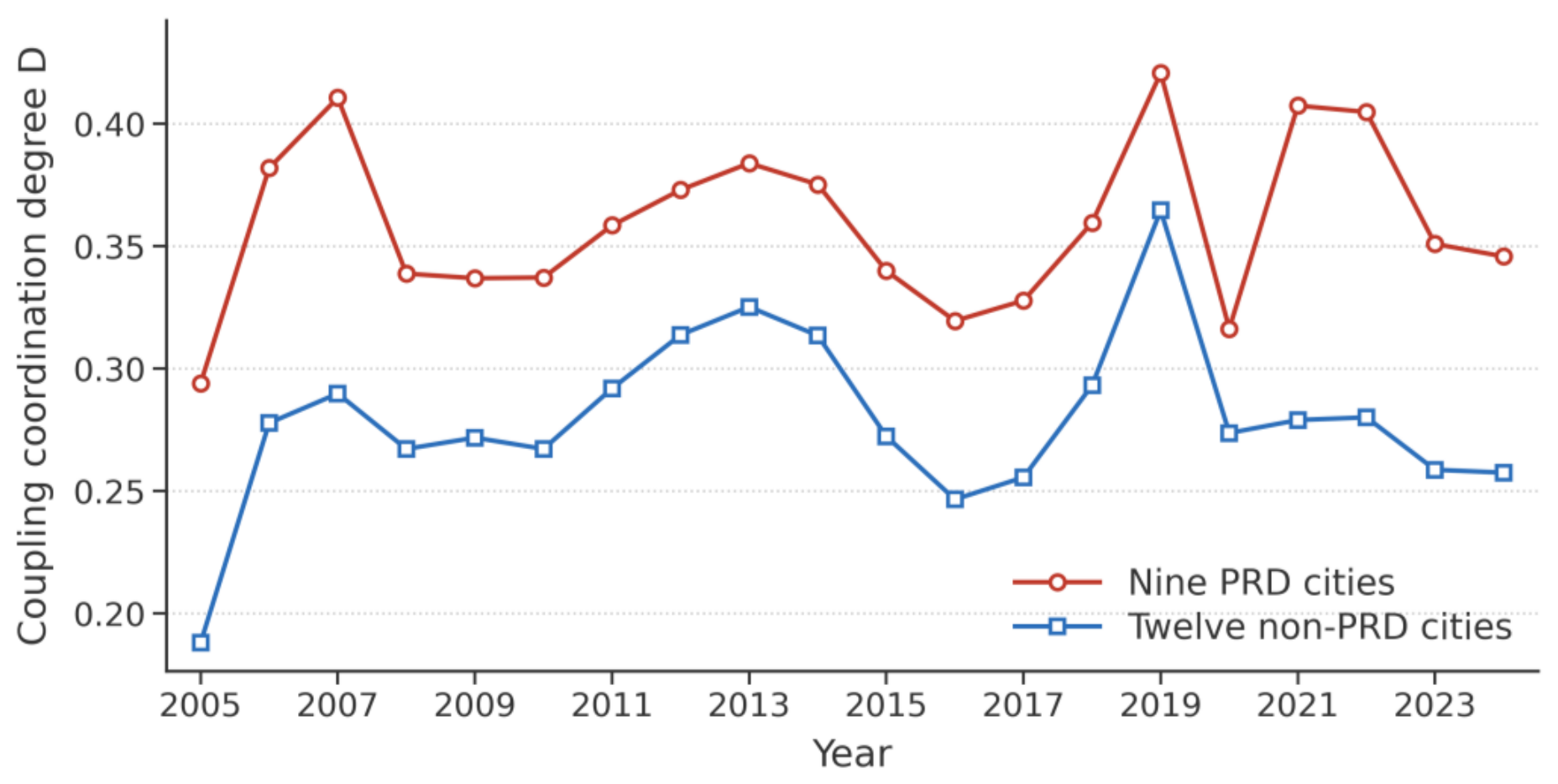
Figure 4.
Dimension-specific effects of REM on urban resilience (two-way fixed effects, city-clustered standard errors).
Figure 4.
Dimension-specific effects of REM on urban resilience (two-way fixed effects, city-clustered standard errors).
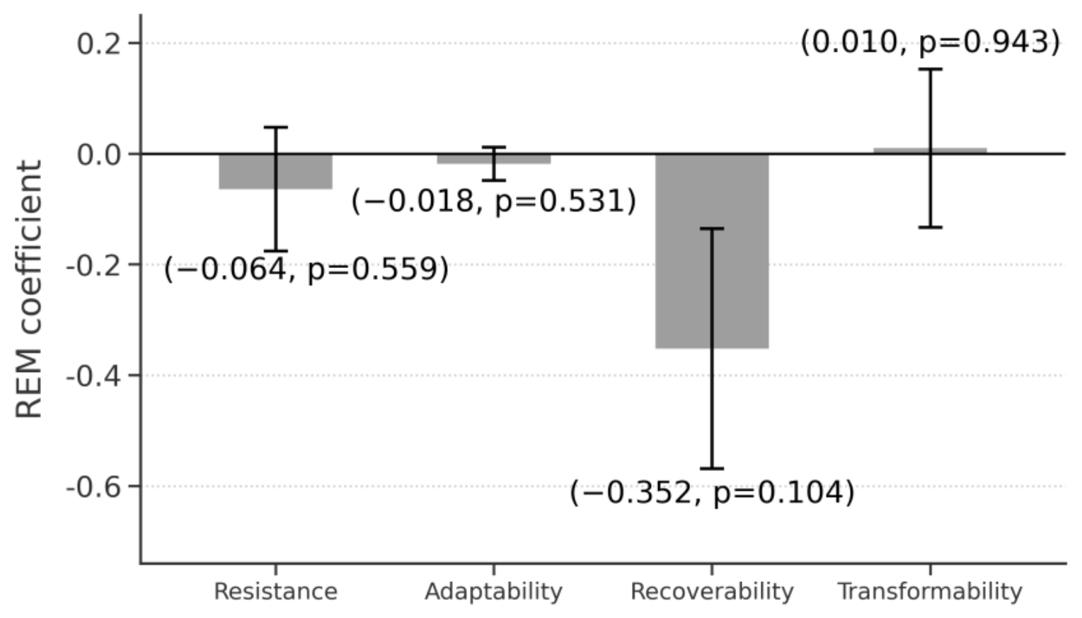

Table 1.
Indicator system for real estate market development.
| Dimension | Indicator | Property |
|---|---|---|
| Market scale | Real estate development investment | Positive |
| Market scale | Share of real estate investment in fixed-asset investment | Moderate/Risk |
| Market price | Average selling price of residential buildings | Moderate |
| Market price | Housing price-to-income ratio | Negative |
| Market supply | Floor space under construction | Positive |
| Market supply | Floor space completed | Positive |
| Market demand | Floor space of commercial buildings sold | Positive |
| Market demand | Resident population growth rate | Positive |
| Financial linkage | Outstanding real estate loan ratio | Moderate/Risk |
| Market risk | Floor space of commercial buildings for sale | Negative |
| Market risk | Housing price volatility | Negative |
Note: “Moderate” and “moderate/risk” indicate that the indicator has a negative effect when it deviates from the desirable range; standardisation follows the attribute classification.
Table 2.
Indicator system for urban resilience.
| Dimension | Indicator | Property |
|---|---|---|
| Resistance | GDP per capita | Positive |
| Resistance | Per capita general public budget revenue | Positive |
| Resistance | Hospital beds per 10,000 people | Positive |
| Adaptation | Tertiary industry share | Positive |
| Adaptation | Urbanisation rate | Positive |
| Adaptation | Per capita road area | Positive |
| Recovery | Registered urban unemployment rate | Negative |
| Recovery | Growth of total retail sales | Positive |
| Recovery | Fiscal expenditure capacity | Positive |
| Transformation | R&D intensity | Positive |
| Transformation | Green coverage rate | Positive |
| Transformation | Digital inclusive finance index | Positive |
Table 3.
Components of the composite uncertainty index.
| Component | Measurement |
|---|---|
| Housing price volatility | Rolling SD of residential price growth |
| Real estate investment volatility | Rolling SD of investment growth |
| Policy uncertainty exposure | National annual EPU index × real estate dependence |
| Fiscal pressure | (Fiscal expenditure − revenue)/revenue |
| External shock | Public health emergency dummy |
| Composite uncertainty | Entropy-weighted aggregation of the above |
Table 4.
Baseline regression and moderating effect of uncertainty.
| Variable | M1: Baseline | M2: Adding UNC | M3: Moderating effect |
|---|---|---|---|
| REM | −0.1451** (0.0631) | −0.1184** (0.0549) | −0.0384 (0.0634) |
| UNC | 0.4522*** (0.0582) | 0.0590 (0.1151) | |
| REM × UNC | 2.1303*** (0.5876) | ||
| lnPGDP | 0.0799** (0.0324) | 0.0789** (0.0329) | 0.0735*** (0.0256) |
| IND | 0.1061*** (0.0303) | 0.0935*** (0.0271) | 0.0987*** (0.0269) |
| lnPOP | 0.1064** (0.0488) | 0.1276*** (0.0486) | 0.0675 (0.0417) |
| N | 420 | 420 | 420 |
| Fixed effects | City + Year | City + Year | City + Year |
Note: City-level clustered robust standard errors in parentheses; ***, **, and * denote significance at the 1%, 5%, and 10% levels. UNC is centred in M3.
Table 5.
Panel threshold estimation results.
| Item | Estimate | p-value |
|---|---|---|
| Threshold variable | UNC | |
| Threshold estimate | 0.0736 | < 0.01 (bootstrap) |
| REM, low-uncertainty regime | −0.1525** | 0.0166 |
| REM, high-uncertainty regime | 0.7516*** | 0.0001 |
| lnPGDP | 0.0696*** | 0.0071 |
| IND | 0.1002*** | 0.0003 |
| N | 420 |
Table 6.
Spatial Durbin model estimates and effect decomposition.
| Item | Estimate | p-value |
|---|---|---|
| LM-lag | 12.9111 | 0.0003 |
| Robust LM-lag | 4.7188 | 0.0298 |
| LM-error | 11.9309 | 0.0006 |
| Robust LM-error | 3.7387 | 0.0532 |
| ρ (spatial autoregressive) | −0.9741*** (0.2498) | 0.0001 |
| W·REM | −0.4706** (0.2286) | 0.0395 |
| IND | 0.0802*** (0.0231) | 0.0005 |
| REM direct effect | −0.1310 | |
| REM indirect effect (spillover) | 0.0682 | |
| REM total effect | −0.0628 |
Note: The spatial weight matrix is row-standardised inverse distance truncated at 500 km; city and year effects included.
Table 7.
Robustness checks.
| Specification | REM coefficient | p-value |
|---|---|---|
| Baseline (M1) | −0.1451 | 0.022 |
| REM replaced by investment intensity | 0.0025 | 0.986 |
| REM replaced by per-capita floor space sold | 0.0054 | 0.552 |
| Adding housing affordability | −0.0067 | 0.506 |
| REM replaced by inverse price volatility | 0.0361 | 0.127 |
| UR by equal weights | −0.0854 | 0.107 |
| UR by principal components | −0.1067 | 0.233 |
| UR proxied by GDP growth stability | −0.0359 | 0.243 |
| Lagged REM (t−1) | −0.1101 | 0.139 |
| Winsorised at 1%/99% | −0.2080 | 0.017 |
| Excluding Guangzhou and Shenzhen | −0.1223 | 0.087 |
| Excluding Guangzhou | −0.1525 | 0.045 |
| Excluding resource-based cities | −0.1393 | 0.029 |
| Excluding population-growth extremes | −0.1281 | 0.030 |
| Placebo (500 permutations): mean | −0.0002 | — |
Disclaimer/Publisher’s Note: The statements, opinions and data contained in all publications are solely those of the individual author(s) and contributor(s) and not of MDPI and/or the editor(s). MDPI and/or the editor(s) disclaim responsibility for any injury to people or property resulting from any ideas, methods, instructions or products referred to in the content. |
© 2026 by the authors. Licensee MDPI, Basel, Switzerland. This article is an open access article distributed under the terms and conditions of the Creative Commons Attribution (CC BY) license.
Copyright: This open access article is published under a Creative Commons CC BY 4.0 license, which permit the free download, distribution, and reuse, provided that the author and preprint are cited in any reuse.