

Submitted:
10 November 2026
Posted:
10 November 2026
You are already at the latest version
Abstract
Q methodology identifies shared patterns in how respondents evaluate sets of statements, but analysis is limited to a few respondents whose number should be lower than that of statements. Moreover, the process can become cumbersome when respondents rank many statements and difficult to reproduce when methodological choices span data preparation, component extraction and interpretation. Generalised Q (GQ) analysis addresses these limitations by constructing synthetic combined statements from smaller sets of constituent statements. Here, we introduce GQR (Generalised Q Analysis in R), an open-source R package implementing the GQ workflow through both a programmatic interface and an interactive Shiny application.GQR supports unrestricted full binary, one-per-group, and random-pattern designs, data transformation and respondent filtering, construction of synthetic evaluation matrices, ordinary and SPSS-compatible principal component analysis (PCA), and regression-based interpretation of both component content and respondent associations. For large ordinary-PCA problems, GQR provides an exact compact method that avoids materialising the synthetic evaluation matrix. The Shiny application uses the same analytical core and can export executable R code recording the current analysis and settings.Computational benchmarks showed that compact PCA reproduced materialised-matrix solutions to numerical precision while reducing runtime and memory requirements by orders of magnitude as the number of synthetic statements and respondents increased. Using the built-in Central and Eastern European gardening dataset, we further demonstrate how GQ analysis can identify multidimensional response patterns and relate them to respondent and garden characteristics. GQR therefore provides an accessible, reproducible and computationally efficient implementation of GQ analysis for multidimensional preference and survey data.
Keywords:
Q methodology
; R package
; computational social science
; shiny
; preference analysis
; questionnaire survey
1. Introduction
Understanding how people organise preferences, attitudes and perceptions across several dimensions is a common problem in the social sciences [1,2]. Conventional variable-centred analyses commonly examine relationships among measured variables across respondents [1], whereas the Q methodology focuses on similarities among respondents in how they evaluate a set of statements [3,4,5]. This respondent-centred approach has been used in psychology [6], political science [7], healthcare [8], regional science [9] and environmental research [10], particularly when the aim is to identify recurring patterns of viewpoints rather than estimate the population frequency of individual responses [1,11].
Traditional Q studies usually ask participants to evaluate or rank a relatively large set of statements, often through a constrained sorting procedure [12,13,14], where the number of participants should be lower than the number of statements. This provides a structured understanding of subjective priorities, but it can become difficult when many statements are included. First, ranking many statements at the same time can place a substantial cognitive burden on respondents, especially when the statements are similar or cover several dimensions. Second, because the conventional Q matrix contains statements in one dimension and respondents in the other, it can support only as many independent respondent dimensions as there are statements. Finally, although the extracted components describe shared patterns among respondents, researchers still need to interpret them from the statements associated with each component [15].
Dentinho, Kourtit and Nijkamp [15] proposed Generalised Q (GQ) analysis to address these limitations. Instead of asking respondents to evaluate every complex statement or combination directly, the method starts with smaller sets of simple statements and constructs combined statements mathematically after data collection. Respondents therefore evaluate a manageable number of constituent statements, while the analysis expands these responses into a much larger set of synthetic statements. Each synthetic statement is defined explicitly by 0/1 dummies that show which original statements are included, retaining a direct link between the extracted components and the statements from which they are built.
This structure also provides a more explicit way to interpret components. After a principal component analysis (PCA), the scores of the synthetic statements can be regressed on the dummies used to construct them. The resulting coefficients show which original statements are most strongly associated with each component. Separately, respondent component loadings can be related to demographic, behavioural or contextual covariates. GQ analysis therefore provides two complementary views of each component: what combination of statements it represents, and which respondent characteristics are associated with it.
Since its introduction, this formulation of GQ analysis has been applied to several distinct empirical problems. Janzakov et al. [16] used the method to examine migration attitudes in Samarkand, Uzbekistan, while Nijkamp et al. [17] applied it to post-conflict infrastructure reconstruction and regional recovery priorities in Iraq. More recent applications have examined residents’ perceptions of traditional gastronomy and its role in tourism development in northern Portugal [18] and visitor perceptions and management priorities across cultural heritage sites in Europe [19]. Together, these studies show that GQ analysis can be used not only for conventional attitude and preference surveys, but also for structured planning and policy problems in which multidimensional response patterns are of interest.
Despite this growing range of applications, GQ analysis still lacks a dedicated open-source implementation covering the complete workflow. Existing studies have therefore relied on study-specific combinations of data preparation, matrix construction and statistical analysis. This becomes increasingly problematic as the number of statements grows because an unrestricted dummy matrix with (m) statements contains (2^m) possible binary combinations, while even grouped designs may produce thousands or tens of thousands of synthetic statements. Reproducible implementation therefore requires not only automated construction of the matrices and subsequent analyses, but computational strategies that avoid unnecessary materialisation and decomposition of very large matrices.
Methodological choices in traditional Q studies vary substantially and are not always reported completely [14]. GQ analysis introduces additional choices, including the synthetic-statement design, transformations, PCA route and interpretation models, which should likewise be recorded explicitly. A code-based implementation can make these decisions reproducible by exposing them as function arguments and by generating a script that records the settings used.
Here, we introduce GQR (Generalised Q Analysis in R), an R [20] package implementing the GQ framework described by Dentinho et al. [15]. GQR provides exported R functions and an interactive Shiny application [21] built on the same analytical core. The package covers data preparation, synthetic-statement design and evaluation, ordinary and SPSS-compatible PCA, Statement–Component Regression, Component–Covariate Regression, visualisation and export. For large ordinary-PCA analyses, GQR can use an exact compact engine that avoids materialising the full synthetic evaluation matrix. The Shiny application can also generate executable R code that records the current analysis and plot settings.
We first describe the basis of Generalised Q analysis and its implementation in GQR, followed by the package architecture, treatment of large synthetic-statement spaces and computational benchmarks. We then demonstrate the workflow using selected variables from the multilingual gardening and biodiversity-awareness dataset of Varga-Szilay et al. [22]. Finally, we discuss the methodological scope, computational limitations and potential uses of GQ analysis in computational social science.
2. Generalised Q Analysis
2.1. From Q Methodology to Synthetic Statements
If n respondents evaluate m simple statements, we can represent these data by V, an n × m respondent-by-statement matrix. Each row contains the evaluations of one respondent, and each column corresponds to one simple statement (Figure 1).
GQ analysis expands the m original statements into k synthetic statements. Their composition is encoded in a k × m binary dummy matrix D: each row represents one synthetic statement, each column represents one original statement, and a value of 1 indicates that the original statement is included in that synthetic statement (0 indicates that it is not included).
For example, the row (1,0,1,0) represents a synthetic statement that contains the first and third original statements but not the second or fourth.
Figure 1.
Conceptual workflow of Generalised Q analysis in GQR: Respondents evaluate simple statements, which are expanded into synthetic statements through the dummy matrix D. The synthetic evaluation matrix W = D Vᵀ is then analysed by PCA, after which interpretation proceeds through statement-based and respondent-based regressions.
Figure 1.
Conceptual workflow of Generalised Q analysis in GQR: Respondents evaluate simple statements, which are expanded into synthetic statements through the dummy matrix D. The synthetic evaluation matrix W = D Vᵀ is then analysed by PCA, after which interpretation proceeds through statement-based and respondent-based regressions.
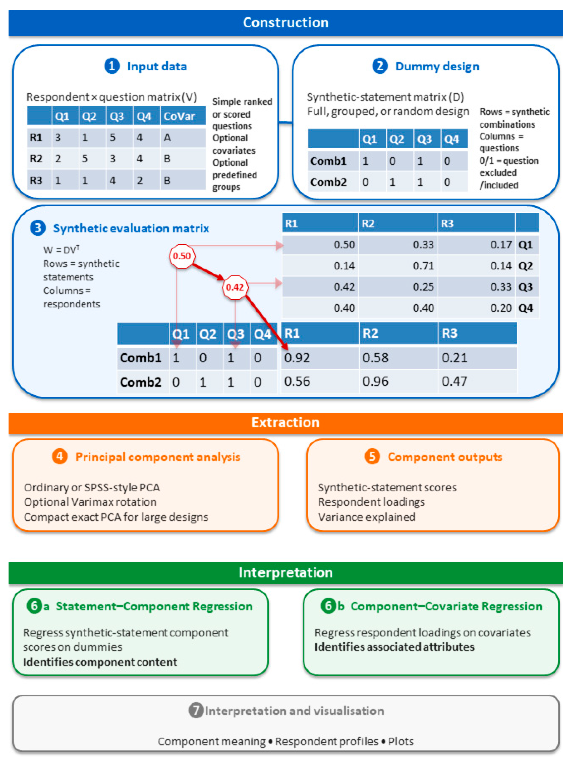
The synthetic evaluation matrix (W) is then obtained as W = DVT, with the resulting W matrix having dimension of k × n. Each value Wij is the synthetic evaluation of statement combination i for respondent j. It is calculated by adding that respondent’s evaluations for all original statements marked 1 in row i of D. A synthetic evaluation is therefore the sum of a respondent’s evaluations of the constituent statements (Figure 1). This additive construction assumes that each constituent statement contributes independently: it does not represent interactions or changes in meaning that arise only when statements are combined. The assumption should therefore be considered when deciding which statements can sensibly be combined and when interpreting the extracted components.
2.2. Construction of the Dummy Matrix
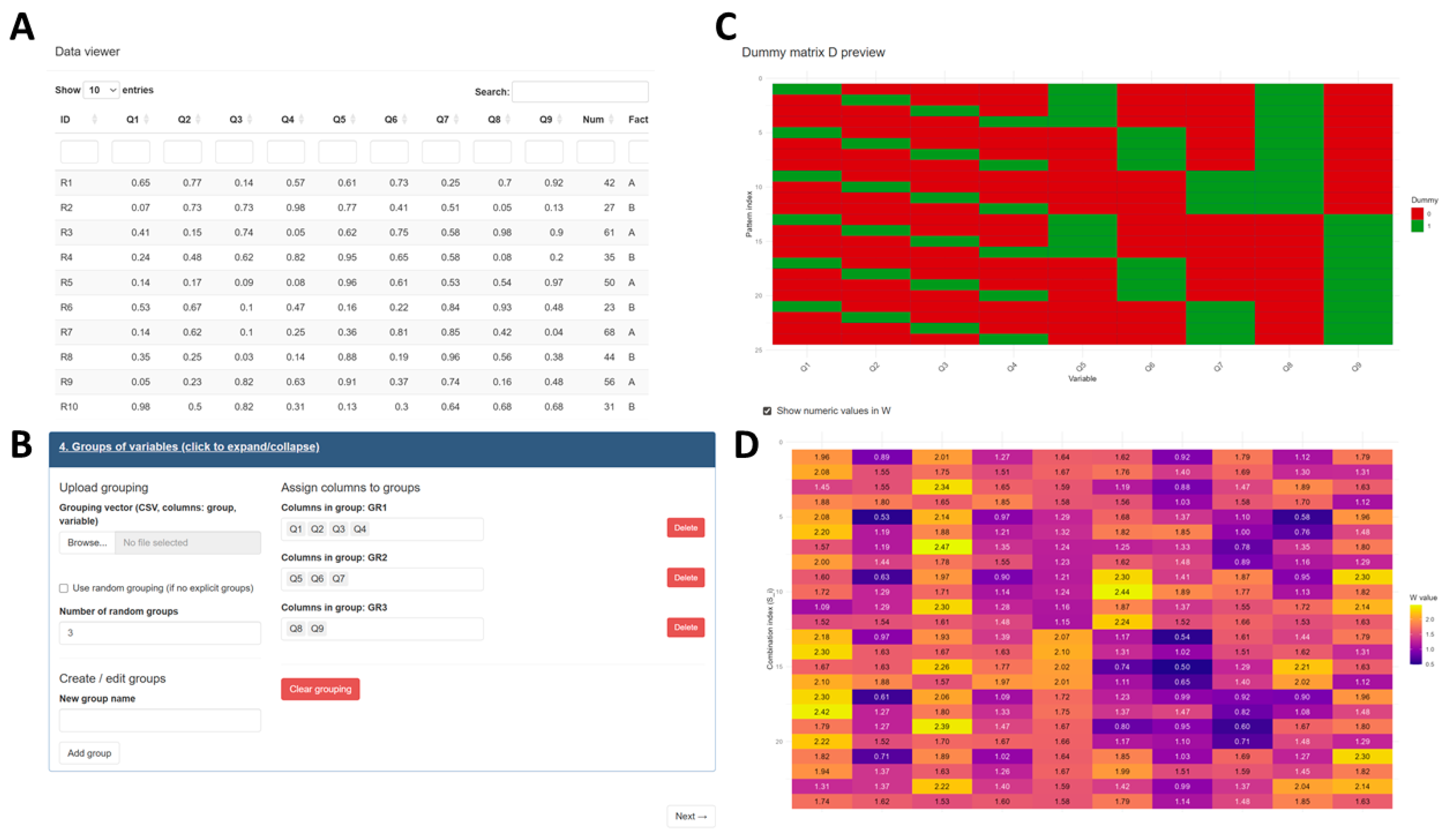
GQR supports three dummy designs through its programmatic interface. In the unrestricted full binary design, every possible 0/1 combination of the m statements is generated, giving k = 2^m synthetic statements. No prior grouping is required, but the design grows exponentially with m. In the grouped one-per-group design, statements are assigned to q conceptually defined groups and each synthetic statement contains exactly one statement from every group (Figure 2). If group g contains rg statements, the number of possible combinations is . This design corresponds most closely to the original GQ formulation, in which alternatives are evaluated within separate questions or thematic domains; when the groups follow the questionnaire structure, it can also reduce the number of synthetic combinations substantially.
The third, random approach generates a user-defined number of randomly sampled synthetic statements rather than constructing the complete set of possible combinations. This provides a Monte Carlo sample of the full binary design space when exhaustive construction is impractical; it does not enforce one statement per thematic group. The Shiny interface currently exposes full and grouped one-per-group designs directly. Its separate “Use random grouping” option randomly assigns analysis variables to groups and then applies the grouped one-per-group design; it should therefore not be confused with the programmatic random-pattern design.
Figure 2.
The data viewer (A), the group selection window (B), the visual representation of the dummy matrix (C), and the visualisation of the weighted W matrix (D), as shown in the GQR Shiny app. The dummy dataset included in the package was used for the figures.
Figure 2.
The data viewer (A), the group selection window (B), the visual representation of the dummy matrix (C), and the visualisation of the weighted W matrix (D), as shown in the GQR Shiny app. The dummy dataset included in the package was used for the figures.
2.3. Principal Component Extraction and Interpretation.
PCA is applied to W to extract the dominant patterns of synthetic-statement evaluations across respondents. GQR supports ordinary centred PCA, with optional scaling, and an SPSS-compatible correlation-based workflow intended to reproduce earlier GQ analyses. The latter uses cor.smooth() and principal() from the psych [23] R package. If the respondent correlation matrix is not positive definite, cor.smooth() adjusts it before component extraction. Varimax rotation can be applied to the retained components in either workflow.
Component interpretation then uses two separate regressions. Statement–Component Regression asks which original statements characterise each component. For each component, synthetic-statement scores are regressed on the 0/1 dummies used to construct the synthetic statements. In grouped one-per-group designs, dummy columns within each group sum to one and cannot all be fitted together with an intercept; GQR therefore omits one statement per group as a reference category, using the first statement in each group by default. The resulting coefficients provide quantitative support for interpreting and/or naming components.
The component–covariate regression asks a different question: which respondent characteristics are associated with each component? Here, respondent component loadings are related to variables such as demographic characteristics, behaviours or spatial categories. The two regressions therefore separate the interpretation of component content from the description of the respondents associated with that component.
3. GQR Implementation
3.1. Package Architecture
GQR is organised around exported analytical functions, with the Shiny application acting as a graphical front end to those functions rather than maintaining a separate calculation engine. Analyses performed through Shiny therefore use the same core implementations available to scripted workflows. The programmatic interface additionally exposes lower-level controls that are not all surfaced in the GUI, including direct random-pattern dummy generation.
The package can be installed from the GitHub repository by using the following R code:
remotes::install_github(“pozsgaig/GQR”, dependencies = TRUE).
The complete scripted workflow can be run with gqr_analysis(). Individual stages, such as data preparation, design estimation, dummy generation, construction of W, PCA and the two interpretation regressions, are also available as separate functions, allowing each step to be controlled or reproduced independently (Table 1). Supporting functions expose data transformation, estimation of synthetic-statement counts and memory requirements, input-file provenance and generation of reproducible analysis scripts.
The Shiny application follows the workflow through six main tabs: Data, Dummies, Principal Component Analysis, Statement–Component Regression, Component–Covariate Regression and Reproducible R script. The Data tab handles input data, column roles, factor designation, transformations and statement grouping. The Dummies tab constructs the dummy matrix and previews synthetic evaluations; the PCA and regression tabs control extraction and interpretation. The final tab converts the current graphical analysis into concise executable R code, recording the data source, final column roles and grouping, transformations, current respondent filters, dummy and PCA settings, regression settings, and the final plot controls. Uploaded files are referenced by their original names, with optional MD5 verification and sessionInfo() output.
GQR requires R (≥ 4.1.0) and keeps the dependencies of its analytical core limited. Most calculations use base or recommended R packages, while psych is required for the SPSS-compatible correlation-based PCA. The optional Shiny interface uses additional packages for data handling, plotting and interactive output. In particular, shiny provides the graphical interface and callr runs computationally intensive operations in separate R processes. The complete dependency list for each release is given in the package DESCRIPTION file.
3.2. Data Preparation and Transformations
GQR accepts ordinary data frames and optional statement-group definitions. gqr_read() reads CSV, RDS and RDA/RData inputs; for CSV files it detects comma, semicolon or tab delimiters, tries common UTF-8 and Windows/Latin encodings, and converts imported headings to deterministic, unique, ASCII, R-compatible names. In Shiny, these imported names can be renamed explicitly and numeric-coded categorical variables can be marked as factors. Analysis-variable and covariate roles are kept mutually exclusive, and factor-marked columns are excluded from the statement set and made available as covariates. Before matrix construction, the preparation functions validate numeric analysis variables, identifiers and the selected roles.
Analysis variables can be standardised, rescaled to the interval [0,1], converted to row-wise relative contributions, or transformed using entropy-based measures, depending on the purpose and structure of the data. Respondent-level variables that are not used to build synthetic statements can be retained as covariates for later Component–Covariate Regression. Keeping analysis variables and covariates separate helps prevent demographic or contextual variables from being included accidentally in the synthetic statements.
3.3. Efficient Analysis of Large Sets of Synthetic Statements
The number of synthetic statements can increase rapidly as m increases, particularly when all binary combinations are allowed. Explicitly constructing the complete synthetic evaluation matrix W = DVᵀ can therefore require substantial memory even when the number of original statements is modest. However, W is obtained by multiplying the k × m dummy matrix D by the m × n transpose of V (VT). Consequently, all variation in W originates from the m original statement columns, and W can contain at most m independent dimensions (Figure 2D), regardless of how many synthetic statements it contains; thus, rank(W) ≤ m.
GQR uses this property in gqr_pca_design(). For ordinary centred/scaled PCA, the main decomposition is performed in the much smaller space defined by the m original statements, and only the required synthetic-statement component scores are reconstructed afterwards. The result is the same as PCA on the fully constructed W matrix to numerical precision, apart from ordinary floating-point differences and the arbitrary sign direction of individual PCA axes. The compact procedure is therefore an exact calculation, not an approximate or randomised form of PCA.
The compact calculation avoids two major computational costs. First, the potentially large W matrix does not need to be stored merely to calculate ordinary PCA. Second, the decomposition is carried out in the much smaller original-statement space and not over all synthetic statements. GQR can select this compact PCA automatically for sufficiently large ordinary-PCA analyses, while users can still request either the full-matrix or compact implementation explicitly.
The SPSS-compatible correlation-based workflow remains separate because it calculates respondent correlations from the materialised W matrix and follows an established scoring convention. GQR therefore retains the full W matrix for this workflow so that its results remain compatible with earlier SPSS-based GQ analyses.
For interactive analyses, GQR estimates the number of synthetic statements and expected memory use before a large ungrouped full-binary calculation begins. Shiny warns users when the requested design is likely to be large and allows them to return to the grouping stage. Moreover, for saving memory, and thus computing time, when W is large, GQR does not plot the complete matrix but previews only the rows required for display. Computationally intensive dummy generation and PCA are run in separate R processes using the callr package [24], so progress can be displayed and a calculation can be stopped without terminating the main Shiny session.
For dense matrix multiplication and decomposition, GQR uses the BLAS/LAPACK numerical libraries supplied with R. Depending on the R installation, these libraries may already use multiple processor cores. GQR therefore prioritises reducing the amount of data that must be stored and processed, rather than creating several R workers that would duplicate large matrices in memory.
3.4. Computational Benchmarking
Computational performance was evaluated with GQR 0.1.2 on two Windows 10 x64 systems: a laptop with a 13th Gen Intel Core i7-1365U processor (10 physical/12 logical cores, 31.7 GB RAM, R 4.5.1) and a PC with an Intel Core i9-14900K processor (24/32 cores, 63.8 GB RAM, R 4.5.0); both used psych 2.5.6. The principal scaling benchmark used unrestricted full binary designs with 6–18 original variables (k = 64–262,144 synthetic statements) and 250, 1,000 or 5,000 respondents. Feasible configurations were repeated three to five times and are summarised by median elapsed time and interquartile range. Ordinary PCA on a materialised W matrix (matrix route) was compared with gqr_pca_design() (compact route). Materialised-W benchmarks were limited to designs requiring no more than approximately 1 GiB, whereas compact runs were continued to larger implied W sizes.
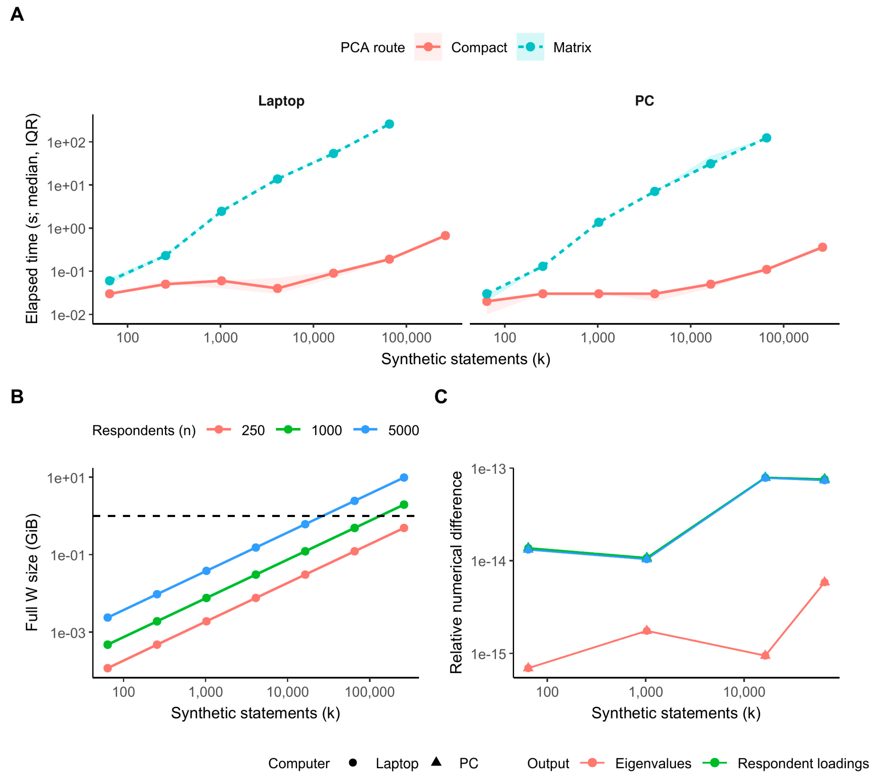
Runtime diverged sharply as the synthetic-statement space and respondent count increased. With 250 respondents and k = 262,144, median compact-PCA time was 0.87 s on the laptop and 0.82 s on the PC, compared with 73.08 s and 41.60 s, respectively, for the matrix route. With 5,000 respondents and k = 16,384, for which a complete W matrix occupies 625 MiB, compact PCA required 0.21 s on the laptop and 0.13 s on the PC, whereas the matrix route required 1,704.86 s and 803.34 s. At k = 262,144 and 5,000 respondents, a complete W matrix would occupy 9.77 GiB; the compact route nevertheless completed in 1.16 s on the laptop and 0.50 s on the PC. Across matched solutions, relative numerical differences in eigenvalues and respondent loadings were on the order of 10−13 or smaller (Figure 3).
Automatic-engine checks produced the same decision on both machines: a 1.95-MB W estimate used the matrix engine and materialised W, whereas a 125-MB estimate selected the compact design engine and did not materialise W, consistent with the 64-MB default thresholds in gqr_analysis().
Figure 3.
Computational performance of GQR 0.1.2. (A) Median elapsed time (IQR) for compact and materialised-matrix ordinary PCA as the number of synthetic statements increased on the laptop and PC. (B) Memory required by a fully materialised W matrix for 250, 1,000 and 5,000 respondents; the dashed line marks the 1-GiB materialised-W benchmark limit. (C) Relative numerical differences between compact and materialised solutions for eigenvalues and respondent loadings; symbols distinguish the two computers.
Figure 3.
Computational performance of GQR 0.1.2. (A) Median elapsed time (IQR) for compact and materialised-matrix ordinary PCA as the number of synthetic statements increased on the laptop and PC. (B) Memory required by a fully materialised W matrix for 250, 1,000 and 5,000 respondents; the dashed line marks the 1-GiB materialised-W benchmark limit. (C) Relative numerical differences between compact and materialised solutions for eigenvalues and respondent loadings; symbols distinguish the two computers.
3.5. Numerical Compatibility and Testing
The package test suite compares compact ordinary PCA with ordinary PCA performed on an explicitly constructed W matrix. Tests account for the arbitrary reversal of individual PCA-axis signs and require eigenvalues, synthetic-statement scores and respondent loadings to agree to numerical precision after sign alignment. The benchmark results above provide an independent scaling check of the same equivalence over much larger designs.
The SPSS-compatible workflow is tested separately because alternative PCA and rotation routines can return mathematically equivalent components in a different order or direction, which would change displayed downstream coefficients. GQR therefore retains psych::cor.smooth() and psych::principal() for this route and validates the established coefficient convention against the bundled synthetic reference example. Across the two benchmark machines, the maximum absolute difference from the reference coefficients was 0.00452.

Table 1.
Principal GQR functions and their role in the Generalised Q workflow.
| Stage | Main function | Principal inputs | Principal output | Shiny tab |
|---|---|---|---|---|
| Data input and preparation |
gqr_read() gqr_prepare_data() gqr_filter_data() (supporting) gqr_transform_data() (supporting) |
File or data frame; analysis, covariate and ID columns; optional transformations and respondent filters. | Data frame or gqr_prepared_data object with validated/transformed data, roles and respondent IDs. | Data |
| Design planning | gqr_estimate_design() | Analysis variables; design mode; optional groups/random-pattern count; respondent count. | Estimated number of combinations and memory required for D and W before allocation. | Data/Dummies |
| Synthetic-statement design | gqr_generate_dummies() | Analysis variables; full, grouped one-per-group or random design; group/random settings. | Binary integer design matrix D, with synthetic combinations in rows and original statements in columns. | Dummies (full/grouped); random via R |
| Synthetic evaluation matrix | gqr_make_w() | Prepared data; analysis columns; D; optional respondent IDs and missing-value handling. | W = D VT, with synthetic statements in rows and respondents in columns; selected rows may be materialised for previews. | Dummies/PCA |
| Component extraction |
gqr_pca() (matrix/SPSS-compatible) gqr_pca_design() (compact exact ordinary PCA) |
W and PCA settings, or prepared data + D for compact PCA; component count; centring/scaling; optional Varimax. | gqr_pca_result with eigenvalues, explained/cumulative variance, synthetic-statement scores, respondent loadings and rotation. | Principal Component Analysis |
| Statement-based interpretation | gqr_regress_statements() | PCA result; D; optional groups, components, standardisation and baselines. | Models and coefficients identifying original statements associated with each component, with baseline/constant-variable information. | Statement-Component Regression |
| Respondent-based interpretation | gqr_regress_respondents() | PCA result; respondent metadata; ID column; numeric/categorical covariates; optional components. | Aligned data, models and coefficients relating respondent component loadings to covariates. | Component-Covariate Regression |
| Complete scripted workflow | gqr_analysis() | Respondent data plus preparation, design, PCA and optional regression settings. | gqr_analysis object with prepared data, design estimates, D, optional W, PCA and optional regressions. | Programmatic interface; orchestrates the same analytical core used by Shiny |
| Graphical workflow | run_gqr() | Optional arguments passed to shiny::runApp(). | Launches the Shiny application; calculations are delegated to the exported gqr_* core functions. | All tabs |
| Code export | gqr_reproducible_script() gqr_file_provenance() |
Frozen analysis state; file provenance; current filters and analysis/plot settings. | Executable R script; optional MD5 verification and sessionInfo(). | Reproducible R script |
Note. gqr_pca() operates on a materialised W matrix and provides both ordinary and SPSS-style correlation PCA, whereas gqr_pca_design() performs algebraically equivalent ordinary PCA directly from D and the original respondent data without requiring the complete W matrix. For large ordinary-PCA analyses, gqr_analysis() can select the compact design engine automatically and avoid retaining W when it is not required. The Shiny interface calls these exported core functions, so graphical and scripted analyses use the same analytical implementations.
4. Application to Gardening Preferences in Central and Eastern Europe.
4.1. Data Source and Analytical Subset
We demonstrate the application of GQR using selected variables from the multilingual garden-management and biodiversity-awareness questionnaire dataset published by Varga-Szilay et al. [22]. The original survey was conducted in nine European countries – Croatia, Czechia, Estonia, Hungary, Latvia, Poland, Romania, Slovakia and Slovenia – and collected information on garden characteristics, management practices, biodiversity-supporting activities and environmental attitudes. Selected variables, and all the original data rows, of this dataset serve as the built-in “gardening” example dataset for the GQR package.
All analyses were conducted using GQR version 0.1.3, using the implemented Shiny app, under R version 4.1.1. The complete analysis script and package version used for the analysis were archived alongside the manuscript.
We loaded the full “gardening” dataset but filtered it for the present demonstration to respondents from Czechia, Estonia, Croatia, Hungary, Slovenia and Slovakia. This six-country subset contained 3,917 rows, compared with 5,511 responses in the full bundled dataset. The example was designed to identify multidimensional configurations among related questionnaire statements and then examine how the resulting component scores varied among respondent and garden characteristics.
4.2. Statement Selection, Grouping and Construction of the GQ Representation
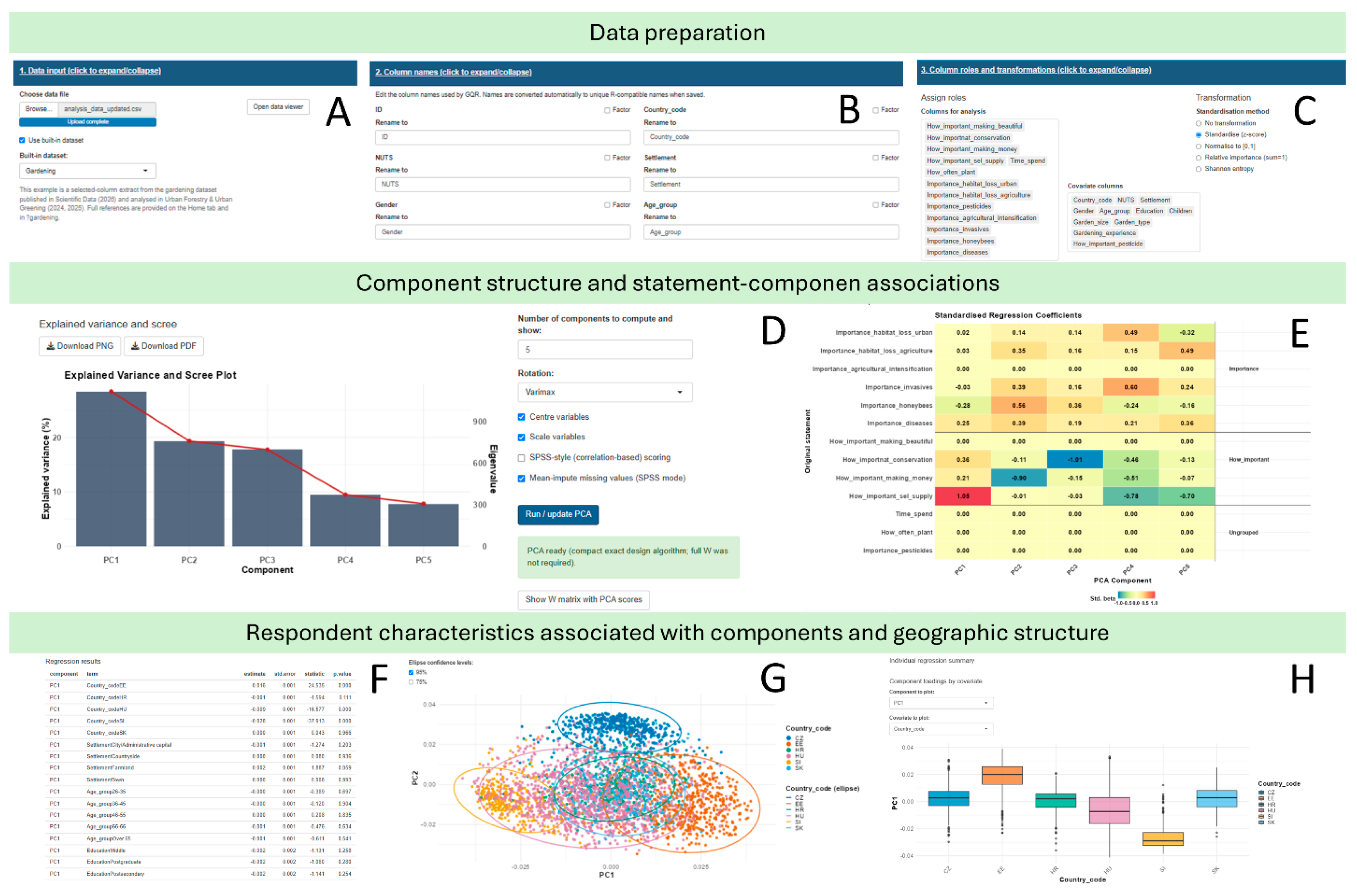
Selected questionnaire statements were used as analysis variables, while respondent- and garden-level characteristics were retained as external covariates (Figure 4A-C). Thirteen variables were included in the GQ analysis. Four statements describing gardening motivations formed one predefined group: beautification, conservation, income generation and self-sufficiency. A second predefined group contained six statements describing perceived pressures on wild pollinators: urban habitat loss, agricultural habitat loss, agricultural intensification, invasive species, honeybees and diseases. The remaining three variables, time spent gardening, planting frequency and pesticides, were retained as ungrouped analysis variables.
The two predefined groups followed the structure of the questionnaire and were specified before examining the component solution, so that the one-per-group combinations reflected sets of conceptually related statements rather than being defined post hoc from the PCA results. The selected analysis variables were standardised using z-scores, after which a grouped one-per-group design was used to construct the GQ representation.
4.3. Principal Component Extraction and Retained Component Structure
Ordinary principal component analysis (PCA) with Varimax rotation was applied to the resulting GQ representation. We initially computed five components, corresponding to the default setting of the GQR Shiny application (Figure 4D), but retained only the first three for subsequent interpretation on the basis of explained variance, the provided scree plot and interpretability of the component structure.
PC1 explained approximately 24% of the total variance, followed by PC2 (approximately 19%) and PC3 (approximately 18%); together, the first three components accounted for approximately 61% of the total variance. The scree plot showed a gradual decline in explained variance across the subsequent components (Figure 4D), supporting the use of the three-component solution for the remaining analyses.
Figure 4.
Graphical user interface of the GQR Shiny application for data preparation and multivariate analysis. Data preparation module, where users can upload a dataset or select an example dataset (A), rename variables, define factor variables (B), specify column roles, and select data transformation and standardisation procedures (C). Group selection and analysis output (D), showing the explained variance and scree plot, together with options for selecting the rotation method (Varimax) and a heatmap of standardized regression coefficients (E). PCA visualisation with user-selectable principal component axes, grouping variables, and graphical representation options, accompanied by the individual regression summary (F-H). The gardening example dataset included in the GQR package was used to generate the displayed results.
Figure 4.
Graphical user interface of the GQR Shiny application for data preparation and multivariate analysis. Data preparation module, where users can upload a dataset or select an example dataset (A), rename variables, define factor variables (B), specify column roles, and select data transformation and standardisation procedures (C). Group selection and analysis output (D), showing the explained variance and scree plot, together with options for selecting the rotation method (Varimax) and a heatmap of standardized regression coefficients (E). PCA visualisation with user-selectable principal component axes, grouping variables, and graphical representation options, accompanied by the individual regression summary (F-H). The gardening example dataset included in the GQR package was used to generate the displayed results.
4.4. Statement–Component Associations and Component Interpretation
After retaining three components, we used Statement–Component Regression to identify the original questionnaire statements most strongly associated with each component (Figure 4E).
PC1 was most strongly and positively associated with the perceived importance of self-sufficiency in the garden (standardised β = 1.05), indicating that this component primarily represented variation along a self-sufficiency dimension. PC2 was strongly negatively associated with the importance of making money from gardening (β = −0.90) and positively associated with the perceived importance of honeybees as a potential negative factor for wild pollinators (β = 0.56). Thus, in the fitted component orientation, higher PC2 scores corresponded to lower emphasis on making money and greater emphasis on the potential negative role of honeybees. PC3 was strongly negatively associated with the importance of conservation-oriented garden management (β = −1.01), so higher PC3 scores corresponded to lower values of this statement. These interpretations were derived from the coefficient patterns rather than imposed from the predefined statement groups.
4.5. Respondent Characteristics and Geographic Structure
We next used Component–Covariate Regression to examine associations between the retained component scores and respondent- and garden-level characteristics, including country, settlement type, age, education, garden size and gardening experience (Figure 4F). For PC1, country showed substantial differences relative to the Czech reference group: Estonia had higher PC1 scores (β = 0.016, p < 0.001), whereas Hungary (β = −0.009, p < 0.001) and Slovenia (β = −0.028, p < 0.001) had lower PC1 scores. Smaller gardens (<10 m2) were also associated with lower PC1 scores (β = −0.002, p = 0.047), while respondents with 2–5 years of gardening experience (β = 0.002, p = 0.030) and 5–10 years of experience (β = 0.002, p = 0.027) showed higher PC1 scores.
The PCA score distributions provided a complementary view of these respondent-level associations (Figure 4G-H). Estonia and Slovenia occupied contrasting positions along PC1, consistent with their positive and negative regression coefficients, respectively. Because PC1 was strongly and positively associated with self-sufficiency, this geographic difference indicates corresponding variation in respondents’ relative position along that dimension. Substantial overlap nevertheless remained among the six countries.
Additional structure was visible on PC2 and PC3. Czech respondents occupied a comparatively distinct position towards positive PC2 values, while Croatian respondents showed higher PC3 scores than most other country groups (Figure 4G). In relation to the Statement–Component Regression results, the positive PC2 position of Czech respondents corresponded to relatively lower values of the making-money statement, whereas higher PC3 scores among Croatian respondents corresponded to relatively lower values of conservation-oriented garden management.
Overall, applying the GQ method to the gardening dataset shows the simplicity of using the Shiny app implemented in the GQR package, and also how GQR can identify multidimensional patterns across related questionnaire statements and subsequently relate those patterns to respondent- and garden-level characteristics. This provides a complementary perspective to previous analyses of the same survey, which have primarily examined associations between socio-demographic characteristics, gardening practices and biodiversity-related management [25,26].
5. Discussion
Our new package, GQR provides the first dedicated R implementation of Generalised Q analysis, bringing the full workflow into a single environment that can be used either interactively or programmatically. Although conventional Q methodology is already supported by tools such as PQMethod [27], the qmethod R package [28] and Ken-Q Analysis [29], GQR was developed specifically for the additional analytical steps required by GQ analysis, including the construction of synthetic statements, their efficient analysis and the subsequent interpretation of the extracted components [15].
Because these additional analytical steps involve several user-defined choices, reproducibility becomes an important consideration. This concern extends across science and has received particular attention in psychology and experimental social science following large-scale replication studies [30,31,32]. Although R provides a fully scriptable and reproducible environment, coding itself remains a barrier to wider use of computational methods in the social sciences [33,34]. GQR therefore combines the R interface with a point-and-click Shiny application, allowing GQ analysis to be carried out without programming while retaining reproducibility. The Shiny application uses the same underlying functions as the scripted workflow and can generate executable R code recording the selected variables, transformations, respondent filters and analytical settings.
The analysis of the built-in gardening dataset further illustrates that the complete workflow, from data preparation and construction of the GQ representation to component interpretation and the analysis of respondent-level covariates, can be carried out directly within the Shiny application. More broadly, this example illustrates that GQ analysis can be applied to existing questionnaire data without requiring a conventional Q-sort, making it potentially useful for secondary analysis of survey datasets where statements can be meaningfully combined. In our example, the three retained axes described variation in self-sufficiency, economic motivation versus recognition of honeybees as a potential pressure on wild pollinators, and conservation-oriented garden management. The second of these was particularly informative: respondents placing greater emphasis on making money from gardening tended to score lower on recognising the potential negative effects of honeybees on wild pollinators, whereas the opposite pattern characterised those more aware of this less intuitive conservation issue. This illustrates how GQ analysis can reveal combinations of attitudes that may remain less apparent when questionnaire items are considered separately.
A practical limitation of GQ analysis is the rapid growth of the synthetic-statement space. Even with a modest number of original statements, exhaustive designs can produce very large W matrices and become computationally demanding. Grouped designs can reduce this growth where the questionnaire structure justifies grouping, while random-pattern designs allow a subset of combinations to be analysed when exhaustive construction is impractical; because both approaches determine which synthetic statements are represented, their use should follow the research question rather than computational convenience alone. GQR also addresses the computational burden of ordinary PCA through its compact implementation. Our benchmarks showed that, as the number of synthetic statements and respondents increased, materialising W rapidly became both slow and memory intensive, whereas the compact approach remained fast even for designs in which the corresponding W matrix would require almost 10 GiB of memory. The compact approach was therefore faster and less memory-intensive because it reformulated the PCA calculation, while it retained a numerically equivalent solution, which, in turn, allows substantially larger GQ designs to be analysed without approximating the PCA solution.
Several limitations remain. First, synthetic evaluations are constructed by adding the values of their constituent statements, which is only appropriate when these statements can be meaningfully combined; interactions or changes in meaning arising from particular combinations are not represented. Second, random-pattern designs analyse only a subset of the possible combination space, and further work is needed to determine how many sampled patterns are required for stable component recovery under different data structures. Finally, although Statement–Component Regression makes the basis of component interpretation more explicit, the resulting coefficients do not determine a unique component label, and substantive judgement remains necessary.
Nonetheless, GQ analysis may be useful beyond attitudinal questionnaires wherever observations can be meaningfully represented as evaluations of constituent attributes and combined through a defined synthetic design. Potential applications include regional and urban preference studies, policy prioritisation, stakeholder analysis, economic structure, and other settings in which multidimensional response profiles rather than isolated variables are of primary interest. The availability of a programmatic interface is particularly relevant for these applications because it allows the method to be incorporated into simulation, resampling and reproducible computational workflows rather than being restricted to interactive analysis.
Software and data availability
GQR is open-source software distributed under the GNU General Public License (GPL ≥ 3). Source code, documentation, vignettes and development history are available from the GitHub repository pozsgaig/GQR. The gardening example uses selected variables from the dataset published by Varga-Szilay et al. (2026). The complete published dataset should be cited independently when the example data or derived analyses are used.
Acknowledgments
We gratefully acknowledge financial support from FCT - Fundação para a Ciência e Tecnologia (Portugal) I.P., in the framework of the unit through research grants UIDB/00685/2025 (https://doi.org/10.54499/UID/00685/2025), CEEAplA | School of Business and Economics of the University of the Azores, and from the Regional Directorate for Science, Innovation and Development – Azores Government through the research grant M1.1. A/FUNC.UI&D/005/2026 (PROSCIENTIA). G.P. was funded by the INTERREG VI D MADEIRA-AÇORES-CANARIAS MAC 2021-2027 (1/MAC/2/2.4/0044). T.P.D. was also supported by the Associação para a Ciência e Desenvolvimento dos Açores (ACDA).
Conflicts of Interest statement
On behalf of all authors, the corresponding author states that there is no conflict of interest.
References
- Howard MC, Hoffman ME (2018) Variable-Centered, Person-Centered, and Person-Specific Approaches: Where Theory Meets the Method. Organizational Research Methods 21:846–876. [CrossRef]
- Woo SE, Hofmans J, Wille B, Tay L (2024) Person-Centered Modeling: Techniques for Studying Associations Between People Rather than Variables. Annual Review of Organizational Psychology and Organizational Behavior 11:453–480. [CrossRef]
- Brown SR (1993) A Primer on Q Methodology. Operant Subjectivity 16:.
- McKeown B, Thomas D (2013) Q Methodology, 2nd ed. SAGE Publications, Inc., Thousand Oaks, California.
- Stephenson W (1953) The study of behavior; Q-technique and its methodology. University of Chicago Press, Chicago, IL, US.
- Rost F (2021) Q-sort methodology: Bridging the divide between qualitative and quantitative. An introduction to an innovative method for psychotherapy research. Counselling and Psychotherapy Research 21:98–106. [CrossRef]
- Nederhand J, Edelenbos J (2023) Legitimate public participation: A Q methodology on the views of politicians. Public Administration Review 83:522–536. [CrossRef]
- Churruca K, Ludlow K, Wu W, Gibbons K, Nguyen HM, Ellis LA, Braithwaite J (2021) A scoping review of Q-methodology in healthcare research. BMC Med Res Methodol 21:125. [CrossRef]
- Pascariu GC, Nijkamp P, Kourtit K (2023) Regional science knowledge needs for the recovery of the Ukrainian spatial economy: A Q-analysis. Regional Science Policy & Practice 15:75–95. [CrossRef]
- Sneegas G, Beckner S, Brannstrom C, Jepson W, Lee K, Seghezzo L (2021) Using Q-methodology in environmental sustainability research: A bibliometric analysis and systematic review. Ecological Economics 180:106864. [CrossRef]
- Zabala A, Sandbrook C, Mukherjee N (2018) When and how to use Q methodology to understand perspectives in conservation research. Conservation Biology 32:1185–1194. [CrossRef]
- Watts S, Stenner P (2005) Doing Q methodology: theory, method and interpretation. Qualitative Research in Psychology 2:67–91. [CrossRef]
- Watts S, Stenner P (2012) Doing Q Methodological Research: Theory, Method and Interpretation. SAGE Publications Ltd.
- Dieteren CM, Patty NJS, Reckers-Droog VT, van Exel J (2023) Methodological choices in applications of Q methodology: A systematic literature review. Social Sciences & Humanities Open 7:100404. [CrossRef]
- Dentinho TP, Kourtit K, Nijkamp P (2023) Generalized Q analysis as a new tool in social science research - a pedagogical introduction. EJES 14:5–21. [CrossRef]
- Janzakov B, Dentinho TP, Akhrorov F (2024) Migrants’ Attitudes from Samarkand, Uzbekistan. A Generalized Q Analysis. RPER 183–196. [CrossRef]
- Nijkamp P, Kourtit K, Dentinho TP (2025) Infrastructure reconstruction planning in post-conflict areas – a multidimensional resilience assessment for Iraq. Planning Practice & Research 40:733–757. [CrossRef]
- Ramazanova M, Freitas IV de, Castro AM, Dentinho TP (2025) Perceptions of Residents of Porto Region on Traditional Gastronomy with a Generalized Q Analysis. RPER 97–113. [CrossRef]
- Kourtit K, Nijkamp P, Gravagnuolo A, Ponce Dentinho T (2026) Managing Cultural Tourism and Heritage Sites in Urban Areas—Application of Q-Analysis to Europe. Urban Science 10:484. [CrossRef]
- R Core Team (2026) R: a language and environment for statistical computing. R Foundation for Statistical Computing, Vienna, Austria.
- Chang W, Cheng J, Allaire J, Xie Y, McPherson J (2020) shiny: Web application framework for r.
- Varga-Szilay Z, Jelaska LŠ, Vilumets S, Barševskis A, Benedek K, Bevk D, Jojczyk A, Krištín A, Růžičková J, Veromann E, Fetykó KG, Szövényi G, Pozsgai G (2026) A multilingual, multi-country dataset on gardening and biodiversity awareness across Central and Eastern Europe. Sci Data. [CrossRef]
- William Revelle (2025) psych: Procedures for psychological, psychometric, and personality research. Northwestern University, Evanston, Illinois.
- Csárdi G, Chang W (2026) callr: Call R from R.
- Varga-Szilay Z, Fetykó KG, Szövényi G, Pozsgai G (2024) Bridging biodiversity and gardening: Unravelling the interplay of socio-demographic factors, garden practices, and garden characteristics. Urban Forestry & Urban Greening 97:128367. [CrossRef]
- Varga-Szilay Z, Barševskis A, Benedek K, Bevk D, Jojczyk A, Krištín A, Růžičková J, Jelaska LŠ, Veromann E, Vilumets S, Fetykó KG, Szövényi G, Pozsgai G (2025) Improving biodiversity in Central and Eastern European gardens needs regionally scaled strategies. Urban Forestry & Urban Greening 113:129074. [CrossRef]
- Schmolck P (2014) PQMethod.
- Zabala A (2015) The R Journal: qmethod: A Package to Explore Human Perspectives Using Q Methodology. The R Journal 6:163–173. [CrossRef]
- Banasick S (2023) Ken-q analysis.
- Open Science Collaboration (2015) Estimating the reproducibility of psychological science. Science 349:aac4716. [CrossRef]
- Camerer CF, Dreber A, Holzmeister F, Ho T-H, Huber J, Johannesson M, Kirchler M, Nave G, Nosek BA, Pfeiffer T, Altmejd A, Buttrick N, Chan T, Chen Y, Forsell E, Gampa A, Heikensten E, Hummer L, Imai T, Isaksson S, Manfredi D, Rose J, Wagenmakers E-J, Wu H (2018) Evaluating the replicability of social science experiments in Nature and Science between 2010 and 2015. Nat Hum Behav 2:637–644. [CrossRef]
- Munafò MR, Nosek BA, Bishop DVM, Button KS, Chambers CD, Percie du Sert N, Simonsohn U, Wagenmakers E-J, Ware JJ, Ioannidis JPA (2017) A manifesto for reproducible science. Nat Hum Behav 1:0021. [CrossRef]
- Wallace BC, Dahabreh IJ, Trikalinos TA, Lau J, Trow P, Schmid CH (2012) Closing the Gap between Methodologists and End-Users: R as a Computational Back-End. Journal of Statistical Software 49:1–15. [CrossRef]
- Abbasnasab Sardareh S, Brown GTL, Denny P (2021) Comparing four contemporary statistical software tools for introductory data science and statistics in the social sciences. Teaching Statistics 43:S157–S172. [CrossRef]
Disclaimer/Publisher’s Note: The statements, opinions and data contained in all publications are solely those of the individual author(s) and contributor(s) and not of MDPI and/or the editor(s). MDPI and/or the editor(s) disclaim responsibility for any injury to people or property resulting from any ideas, methods, instructions or products referred to in the content. |
© 2026 by the authors. Licensee MDPI, Basel, Switzerland. This article is an open access article distributed under the terms and conditions of the Creative Commons Attribution (CC BY) license (http://creativecommons.org/licenses/by/4.0/).
Copyright: This open access article is published under a Creative Commons CC BY 4.0 license, which permit the free download, distribution, and reuse, provided that the author and preprint are cited in any reuse.