Quantification of the Energy Radiated by a Low-Frequency Electrical Circuit with a Nonlinear Load and Non-Harmonic Supply

1. Introduction

Modern electrical appliances equipped with electronic control systems or power regulation are widely used in environments where people spend extended periods of time. The theory of electromagnetic field (EMF) propagation at frequencies associated with commercially available devices has been addressed in numerous areas of research. At frequencies above 100 kHz, various analyses are available concerning the effects of EMF, including its effects on the human body [2,3]. In contrast, the low-frequency range below 100 kHz has received considerably less research attention from this perspective. A similar situation exists in the extremely low frequency (ELF) range, typically in the order of tens of hertz.

With the introduction of modern energy-efficient lighting technologies, extra-low-voltage (ELV) electrical installations operating at voltages up to 60 V have become increasingly common. However, transferring the same amount of energy from a 50/60 Hz public electricity supply to a load operating at 24 V requires a direct current in the conductors that can be approximately ten times higher. When the power delivered to the load is simultaneously regulated using pulse-width modulation (PWM), interesting phenomena involving higher-order harmonic components arise both in the supply wiring and within the load itself.

Since the conductors and electrical appliances used in such applications are commonly installed in occupied environments, often in close proximity to people, the energy radiated by the resulting electromagnetic field may reach non-negligible levels. According to the well-established mathematical relationship describing the EMF, namely the energy balance equation [1], a portion of the useful energy supplied to a closed system is converted into Joule heat, while the remaining portion is radiated into the surrounding environment. The experiment demonstrates that the presence of higher-order harmonic components in the supply voltage alters this energy distribution. As the frequency increases, the energy associated with the generated electromagnetic wave also increases. At low frequencies, this energy is relatively small and is therefore often considered negligible in calculations. The objective of this study is to quantify the amount of radiated energy in circuits operating within the ELF range, particularly with regard to the generation and presence of higher-order harmonic components.

The theoretical part of the article focuses on describing the power supply method and calculating the actual energy delivered to the electrical load. The nonlinear nature of the load and the theoretically justified generation of significant higher-order harmonic components are described up to frequencies in the order of 100 kHz. The circuit is supplied with direct voltage, which is switched to regulate the power delivered to the load. The switching is performed using PWM, resulting in a non-sinusoidal supply waveform.

The objective of the experimental part of this study is to confirm the existence of, and practically quantify, the EMF generated when low-voltage electrical appliances are powered using PWM. For the purposes of this study, experimental measurements were performed using a DC power supply with a PWM output, operating at switching frequencies of 1,400 Hz and 4,000 Hz and employing different modulation depths φ.

2. Materials and Methods

A. Principle of the Experiment

We start from the generally applicable energy balance equation, expressed in the form given by (1)

$${\displaystyle \underset{\mathit{V}}{\int }}\left({\displaystyle \frac{1}{2}}\epsilon E^2+{\displaystyle \frac{1}{2}}\mathrm{\mu }{H}^2\right)\mathit{dV}={\displaystyle \underset{\mathit{V}}{\int }}\gamma E^2\mathrm{d}V+{\displaystyle \underset{\mathit{S}}{\oint }}\left(\mathbf{E}\mathit{x}\mathbf{H}\right).\mathbf{dS}$$

(1)

which describes the amount of energy supplied to a system and the mechanisms by which this energy is converted into other forms. The validity of this equation can also be demonstrated for anisotropic and inhomogeneous media. However, it does not hold for nonlinear media in which the material parameters ε, µ, γ are functions of the electric and magnetic field intensities, E and H or of time t.

In the present case, the left-hand side of the equation represents the energy supplied to a closed volume over a specified period of time, which can be precisely defined and experimentally implemented. The right-hand side describes the Joule heat, which can be measured experimentally, while the remaining term represents the energy radiated into the surrounding environment.

For the steady-state condition, when the system is supplied with direct voltage in the first case, the following relationship applies:

$${\displaystyle \underset{\mathit{S}}{\oint }}\left(\mathbf{E}\mathit{x}\mathbf{H}\right).\mathbf{dS}=0$$

(2)

and the left-hand side of the equation (1) $-{\displaystyle \frac{\partial }{\partial t}}{\displaystyle \underset{V}{\int }}\left({\displaystyle \frac{1}{2}}\epsilon E^2+{\displaystyle \frac{1}{2}}\mu H^2\right)\mathrm{d}V$ is constant. Therefore, ${\mathrm{J}}_1={\displaystyle \underset{V}{\int }}\gamma {\mathrm{E}}^2\mathit{dV}$ let us denote it as the Joule heat generated in the first case. In the second case, involving a nonlinear power supply, the corresponding quantity will similarly be ${\mathrm{J}}_2={\displaystyle \underset{V}{\int }}\gamma {\mathrm{E}}^2\mathrm{dV}$ The energy supplied in both cases is kept equal; therefore, the following relationship holds:

$$J_1={\displaystyle \underset{\mathit{V}}{\int }}\mathit{\gamma }{E}^2\mathbf{d}V\mathbf{a}{J}_2={\displaystyle \underset{\mathit{V}}{\int }}\mathit{\gamma }{E}^2\mathbf{d}V+{\displaystyle \underset{\mathit{S}}{\oint }}\left(\mathbf{E}\mathit{x}\mathbf{H}\right).\mathbf{dS}$$

(3)

Since J₁ = J₂ the expression therefore becomes

$${\mathit{Q}}_{\mathit{v}}={\displaystyle \underset{\mathit{S}}{\oint }}\left(\mathbf{E}\mathit{x}\mathbf{H}\right).\mathbf{dS}$$

(4)

represents the amount of energy radiated into the surrounding space through the closed surface S. It is a scalar quantity obtained from the scalar product of the differential surface element dS and the vector product (ExH). To calculate the total energy supplied to the entire measurement system, the heat capacity of the system c, must be known. The following relationship applies:

$$Q_{\mathbf{S}}=\mathit{c}\mathit{\Delta }{\mathsf{\vartheta }}_{\mathit{S}}=U_{\mathit{S}}{I}_S{\mathbf{T}}_0$$

(5)

where Q_S is the energy supplied to the system under steady-state conditions [Ws], $\Delta {\mathsf{\vartheta }}_{\mathrm{S}}$ [K] is the temperature change resulting from the energy supplied to the measurement system over a period of time T₀ [s] a c [JK⁻¹] is the heat capacity of the measurement system. The value of Q_v will be zero under steady-state conditions, since the system is supplied with direct voltage and all the supplied energy is converted into Joule heat, resulting in an increase in temperature of [missing symbol]. Therefore, for measurement and subsequent calculations, if the amount of energy Q supplied to the system and the resulting temperature change $\Delta \mathsf{\vartheta }$ are known, the following relationship applies:

$$\mathit{c}={\displaystyle \frac{{\mathit{Q}}_{\mathbf{S}}}{\Delta {\vartheta }_S}}={\displaystyle \frac{U_S{I}_S{\mathbf{T}}_0}{\Delta {\vartheta }_S}}$$

(6)

Equation (6) is valid under the assumption that the same measurement system is used throughout, with an unchanged mass, material composition, and corresponding heat capacity c [WsK⁻¹]. The value of c_S represents the amount of energy required to increase the temperature of the measurement system by one Kelvin. It is advisable to choose value Δϑ as high as possible, which in practical terms means conducting the measurement over a longer period of time, thereby achieving higher measurement accuracy. Consequently, for the expression in (4), the following relationship applies:

$${\mathrm{Q}}_{\mathrm{N}}=c\Delta {\mathsf{\vartheta }}_{\mathrm{N}}+{\mathrm{Q}}_{\mathrm{V}}={\mathrm{Q}}_{\mathrm{S}}$$

(7)

where Q_N is the energy supplied to the system under transient conditions (non-stationary system) when powered by a non-sinusoidal source, and $\Delta {\mathsf{\vartheta }}_N$ is the resulting temperature change caused by this energy. For convenience, we choose Q_N = Q_S, and after substituting c from equation (6), we obtain:

$$c\left(\Delta {\mathsf{\vartheta }}_{\mathrm{S}}-\Delta {\mathsf{\vartheta }}_{\mathrm{N}}\right)={\mathrm{Q}}_v$$

(8)

Equation (8) expresses the amount of energy radiated into the surrounding space [Ws]. Since the same measurement system is investigated, only the differences in temperature rise are considered. Equation (8) can therefore be regarded as an alternative form of the energy balance equation (1), applicable to the investigated system described above.

B. Characteristics of the Nonlinear Load

For clarity, the nonlinear load, which is a source of additional distortion of the supply current, is described using an equivalent circuit. In the present study, the load consists of a commercially available standard LED strip incorporating semiconductor LED chips connected in a voltage-driven configuration. The current flowing through the strip is in the order of 10 A, and its total length is 10 m.

Figure 1. Equivalent circuit of the analysed load.

Figure 1. Equivalent circuit of the analysed load.

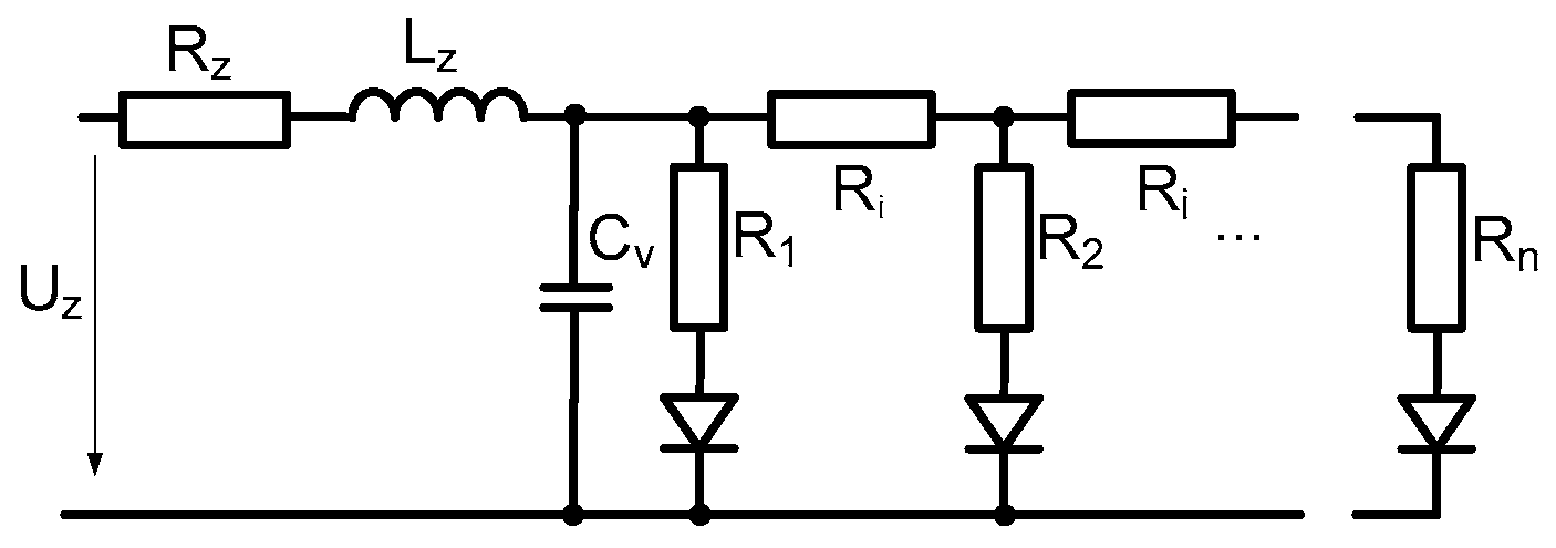
As evident from the equivalent circuit shown in Figure 1, an analytical description of the load characteristics based solely on calculations is not straightforward, particularly given the presence of several hundred semiconductor components. Such an approach would require the adoption of several simplifying assumptions. A closer approximation of the actual characteristics can be achieved through measurements, followed by an analytical representation of the general nonlinear load characteristics using a Lagrange interpolation polynomial [5].

In practical applications, the Shockley equation [4] is commonly used to describe the behaviour of a semiconductor diode with sufficient accuracy. It describes the current flowing through the diode as a function of the applied voltage (9):

$${\mathit{I}}_{\mathbf{FS}}=\left({\mathit{I}}_0.{\mathit{e}}^{{\displaystyle \frac{{\mathit{U}}_{\mathbf{F}}}{\mathbf{n}.{\mathbf{U}}_{\mathbf{T}}}}}-1\right)$$

(9)

and

$${\mathbf{U}}_{\mathbf{T}}={\displaystyle \frac{\mathbf{kT}}{\mathbf{q}}}$$

(10)

where I_FS is the calculated current flowing through measured diode [A], I₀ is the reverse saturation current [A], q is the elementary charge 1,602.10⁻¹⁹[C], U_F is the forward voltage across the diode [V], k is the Boltzmann constant 1.38.10⁻²³[J/K], n is the ideality factor, with values in the range of <1,2>, and T is the absolute temperature [K]. The measured I_F and calculated I_FS values are presented in Table I

Table 1. Selected Measured and Calculated Values of the Voltage–Current (VA) Characteristic of the Nonlinear Element.

UF[V]	IF[mA]	UF[V]	IF[mA]	UF[V]	IF[mA]	UF[V]]	IF[mA]	UF[V]	IF[mA]
0.2	60	3.2	273	6.2	348	9.2	557	12.2	3134
0.4	80	3.4	291	6.4	331	9.4	599	12.4	3652
0.6	100	3.6	311	6.6	333	9.6	638	12.6	4266
0.8	100	3.8	332	6.8	340	9.8	687	12.8	4992
1.0	101	4.0	342	7.0	345	10.0	756	13.0	5851
1.2	102	4.2	343	7.2	352	10.2	837	13.2	6867
1.4	102	4.4	344	7.4	350	10.4	934
1.6	103	4.6	345	7.6	369	10.6	1048
1.8	112	4.8	346	7.8	390	10.8	1183
2.0	130	5.0	346	8.0	403	11.0	1343
2.2	201	5.2	347	8.2	418	11.2	1523
2.4	202	5.4	349	8.4	436	11.4	1746
2.6	210	5.6	351	8.6	457	11.6	2011
2.8	228	5.8	353	8.8	482	11.8	2325
3.0	251	6.0	355	9.0	512	12.0	2695

Table 1. Selected Measured and Calculated Values of the Voltage–Current (VA) Characteristic of the Nonlinear Element.

UF[V]	IF[mA]	UF[V]	IF[mA]	UF[V]	IF[mA]	UF[V]]	IF[mA]	UF[V]	IF[mA]
0.2	60	3.2	273	6.2	348	9.2	557	12.2	3134
0.4	80	3.4	291	6.4	331	9.4	599	12.4	3652
0.6	100	3.6	311	6.6	333	9.6	638	12.6	4266
0.8	100	3.8	332	6.8	340	9.8	687	12.8	4992
1.0	101	4.0	342	7.0	345	10.0	756	13.0	5851
1.2	102	4.2	343	7.2	352	10.2	837	13.2	6867
1.4	102	4.4	344	7.4	350	10.4	934
1.6	103	4.6	345	7.6	369	10.6	1048
1.8	112	4.8	346	7.8	390	10.8	1183
2.0	130	5.0	346	8.0	403	11.0	1343
2.2	201	5.2	347	8.2	418	11.2	1523
2.4	202	5.4	349	8.4	436	11.4	1746
2.6	210	5.6	351	8.6	457	11.6	2011
2.8	228	5.8	353	8.8	482	11.8	2325
3.0	251	6.0	355	9.0	512	12.0	2695

Figure 2. (a) Graphical representation of the Shockley equation and measured values for the analysed semiconductor chip acting as a nonlinear load. (b) Graphical representation of the measured values of the actual nonlinear load.

Figure 2. (a) Graphical representation of the Shockley equation and measured values for the analysed semiconductor chip acting as a nonlinear load. (b) Graphical representation of the measured values of the actual nonlinear load.

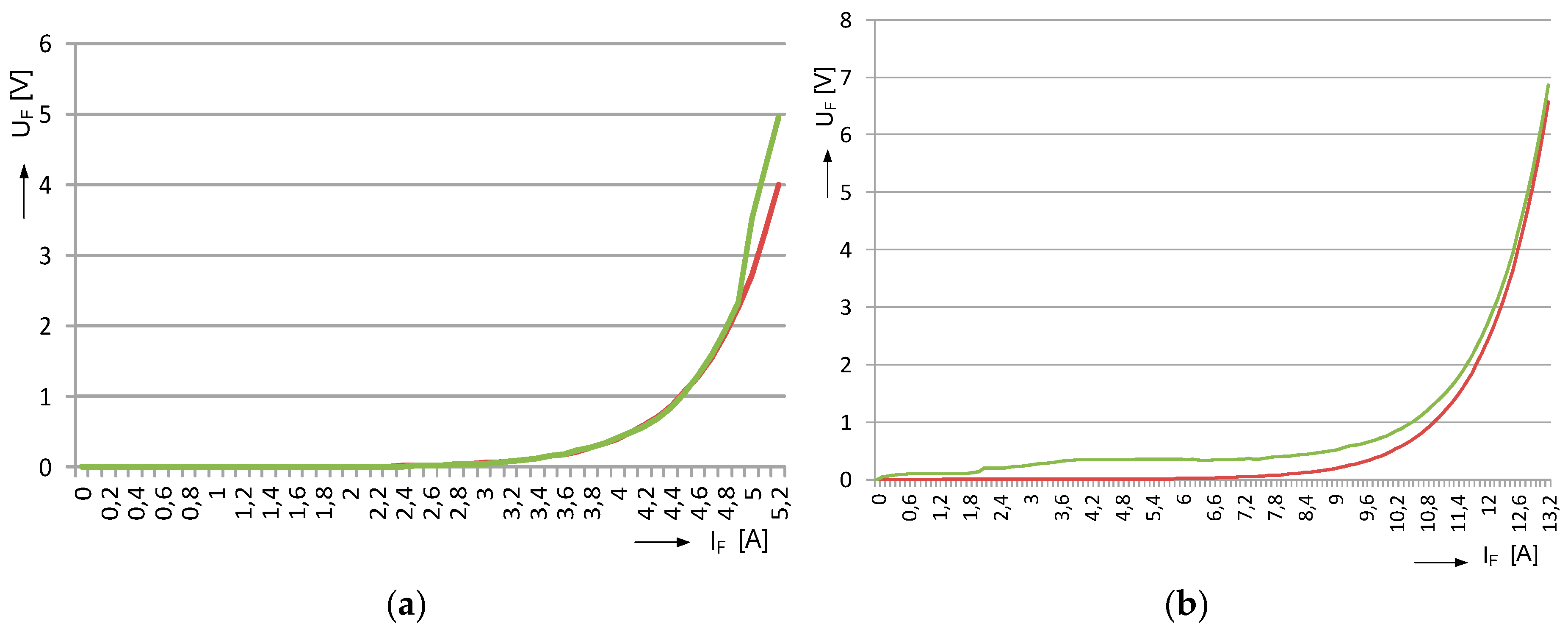
The graphical representation of the measured values of I_F and U_F , together with the values obtained from the Shockley function I_FS=f(U_F), shown in Figure 2(a), clearly demonstrates significant nonlinearity in both the theoretical analysis and the experimental measurements. Figure 2(b) presents a graphical representation of the voltage–current (VA) characteristics of the actual nonlinear load shown in Figure 1. The measured values are provided in Table II, where U_F [V] represents voltage values ranging from 0 to 110% of the nominal DC operating voltage, and I_F [mA] represents the corresponding current values in the circuit.

The graphical representation of the VA characteristic reveals similar nonlinear behaviour. It can therefore be expected that the analysed practical load, when supplied with the voltage waveform shown in Figure 3, will generate higher-order harmonic components. Experimental verification and quantification of this phenomenon constitute the subject of the present study.

Table 2. Selected Measured and Calculated Values of the Voltage–Current (VA) Characteristic of the Nonlinear Element.

UF[V]	IF[mA]	IFS[mA]	UF[V]	IF[mA]	IFS[mA]
0.1	1.04	0.04	1.4	7.68	2.67
0.2	1.09	0.09	1.6	9.01	4.01
0.3	1.15	0.15	1.8	11.97	5.96
0.4	1.23	0.22	2.0	data	8.82
0.5	1.32	0.31	2.2	data	13.01
0.6	1.43	0.42	2.4	data	19.13
0.7	1.56	0.56	2.6	data	28.10
0.8	3.42	0.72	2.8	data	41.22
0.9	3.91	0.91	3.0	data	60.43
1.0	6.14	1.14	3.2	data	88.54
1.1	6.43	1.42	3.4	data	129.6
1.2	6.77	1.76	3.6	data	189.9
1.3	7.18	2.17	3.8	data	278.0

Table 2. Selected Measured and Calculated Values of the Voltage–Current (VA) Characteristic of the Nonlinear Element.

UF[V]	IF[mA]	IFS[mA]	UF[V]	IF[mA]	IFS[mA]
0.1	1.04	0.04	1.4	7.68	2.67
0.2	1.09	0.09	1.6	9.01	4.01
0.3	1.15	0.15	1.8	11.97	5.96
0.4	1.23	0.22	2.0	data	8.82
0.5	1.32	0.31	2.2	data	13.01
0.6	1.43	0.42	2.4	data	19.13
0.7	1.56	0.56	2.6	data	28.10
0.8	3.42	0.72	2.8	data	41.22
0.9	3.91	0.91	3.0	data	60.43
1.0	6.14	1.14	3.2	data	88.54
1.1	6.43	1.42	3.4	data	129.6
1.2	6.77	1.76	3.6	data	189.9
1.3	7.18	2.17	3.8	data	278.0

C. Characteristics of Non-Sinusoidal Power Supply

For the analytical description of the power supply voltage waveform, well-established relationships are used (10-12) [6]. The waveform is a commonly studied non-sinusoidal PWM signal, whose characteristics vary depending on the modulation depth φ.

Figure 3. Voltage and current waveforms at the terminals of a PWM power supply [14, 16] with a modulation depth of 20%.

Figure 3. Voltage and current waveforms at the terminals of a PWM power supply [14, 16] with a modulation depth of 20%.

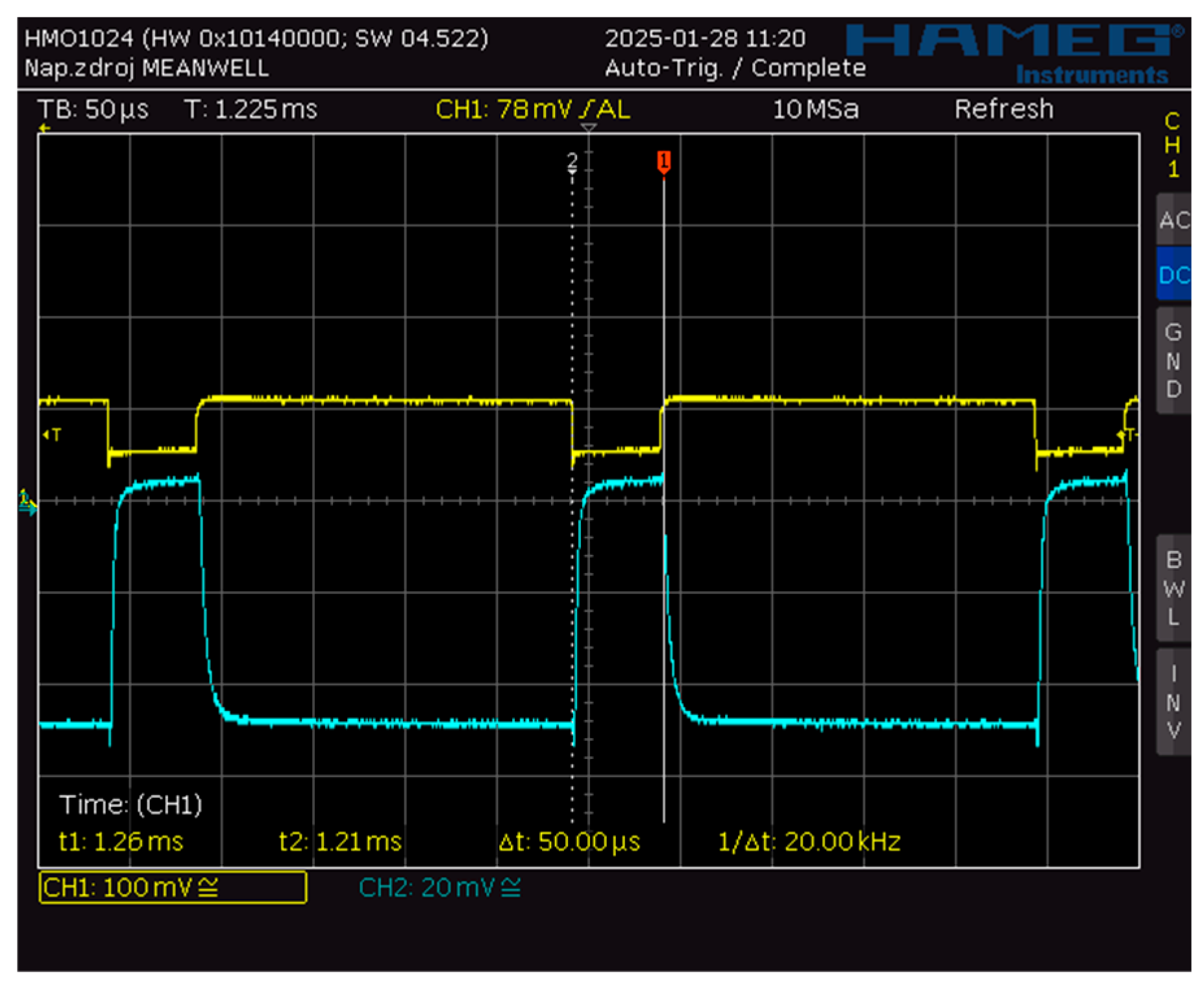
The time-dependent asymmetric supply voltage waveform shown in Figure 4, with a modulation depth of φ = t_i/T, is described for calculation and graphical representation purposes using the first form of the Fourier series.

For further analysis and substitution into equation (11), the voltage u(t) needs to be expressed in the following form:

$$\mathit{u}\left(\mathit{t}\right)={\mathbf{U}}_0+{\displaystyle \sum _{\mathit{k}=1}^{\mathit{n}}}{\mathbf{U}}_{\mathbf{m}\left(\mathbf{k}\right)}\mathbf{sin}\left(\mathit{k}\mathit{\omega }\mathit{t}+{\mathit{\psi }}_{\left(\mathit{k}\right)}\right)$$

(11)

$${\mathbf{U}}_{\mathit{m}\left(\mathit{k}\right)}=\sqrt{{\mathbf{A}}_{\left(\mathit{k}\right)}^2+{\mathbf{B}}_{\left(\mathit{k}\right)}^2}$$

(12)

$$\mathit{tg}{\mathit{\psi }}_{\left(\mathit{k}\right)}={\displaystyle \frac{\mathbf{sin}\left(\mathit{k}\mathit{\omega }\mathit{t}\right)}{1-\mathbf{cos}\left(\mathit{k}\mathit{\omega }\mathit{t}\right)}}$$

(13)

In the specific case of supplying the load with an ideal PWM voltage waveform, the load operates only at the maximum voltage level. Accordingly, during the interval Δt=<0,t_i>, the current, as shown in Figure 4, corresponds to the current value I_m at the given U_m. During the interval <t_i,T> the current is zero. Consequently, the nonlinear characteristics of the load do not become apparent.

Figure 4. Harmonic components of the power supply voltage under no-load conditions.

Figure 4. Harmonic components of the power supply voltage under no-load conditions.

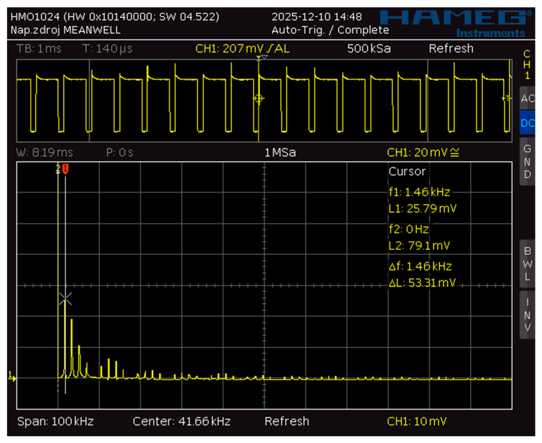
A different situation arises when the load is supplied with a general non-sinusoidal voltage waveform, in which case the imperfections of the switching element also become apparent. Consequently, an analytical description of the current waveform in the circuit becomes more complex.

Figure 5. Harmonic components of the voltage and current waveforms in a circuit loaded with a nonlinear load.

Figure 5. Harmonic components of the voltage and current waveforms in a circuit loaded with a nonlinear load.

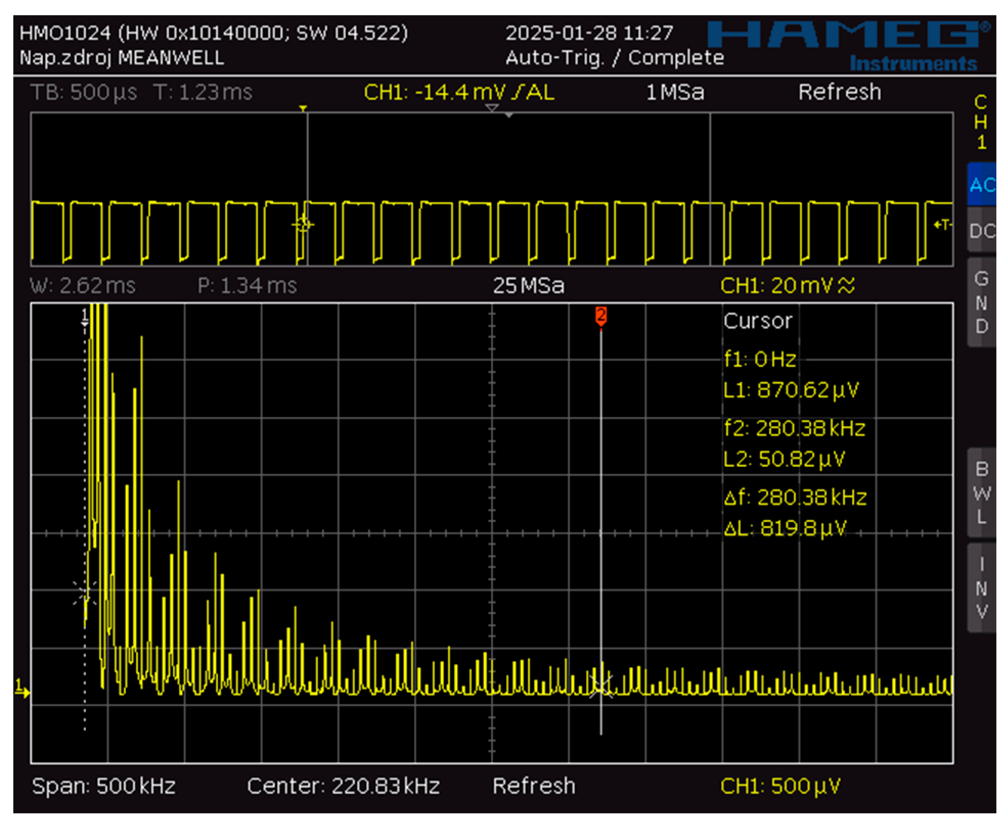
Figure 5 allows the complexity of the current waveform flowing through the circuit and its harmonic content to be assessed. By visualizing the presence of higher-order harmonic components, the experimental setup enables the investigation of system behaviour under variations in modulation depth, frequency, and, if required, supply voltage amplitude.

3. Results

For the experiment to provide sufficiently reliable and meaningful results, the following assumptions must be satisfied:

The experiment must be conducted over a sufficiently long period of time, on the order of several hours, in order to minimise measurement errors.

Both measurements must be performed using the same test specimen.

The length of the connecting wires between the power supply and the load must be negligible compared with the length of the load, which represents the active region contributing to electromagnetic radiation.

The nonlinear load under investigation, namely the LED strip, must be positioned in such a way that it does not form closed loops, thereby preventing the introduction of parasitic inductance that would not be representative of real-world operating conditions.

Measurements must be performed in an actual room where electromagnetic noise is naturally present. Care must be taken to ensure that the noise level remains approximately constant throughout the entire measurement period, thus maintaining equivalent measurement conditions in this respect.

The nonlinear load under investigation must not exhibit significant thermal inertia.

Despite effective thermal insulation of the measurement system from its surroundings, a small amount of heat inevitably escapes from the system. Additional measurement errors may arise from power losses in the connecting wires and other sources. It is therefore essential to use the same measurement system for both measurements and to satisfy assumptions 1–3. Under these conditions, such errors become systematic, and it can be assumed that their effects are approximately equal in both measurements.

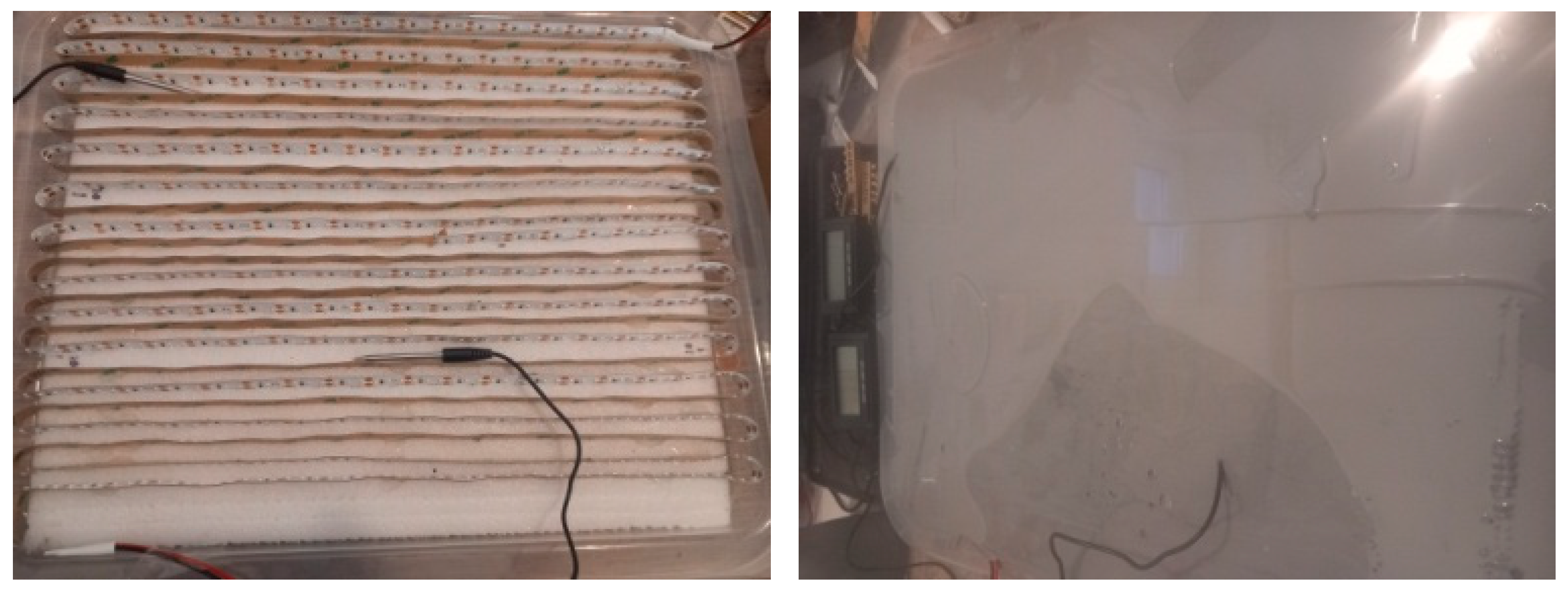
The load itself is embedded in a material that ensures heat transfer and a uniform temperature distribution while simultaneously allowing energy to propagate into the surrounding space. The manufacturer of the material intended for medical applications [7] specifies its permittivity ε, and other material parameters.

Figure 6. Measured load after placement in the template (with indication of the location of the temperature probes) and after pouring with a homogeneous heat-conducting material.

Figure 6. Measured load after placement in the template (with indication of the location of the temperature probes) and after pouring with a homogeneous heat-conducting material.

Measurement Procedure:

1. DC current with precisely defined characteristics, according to Equation (6), is applied to the input of the system. A specified amount of energy (5) is supplied to the circuit over a time interval T₀ during which the temperature of the system increases by Δϑ The measured value is presented in Table II. The measurement can be performed for different values of time T₀

2. After thermal equilibrium has been reached at temperature ϑ₁ and a sufficient time has elapsed since the measurement described in Step 1, a PWM voltage with the characteristics specified in Table IV is applied to the input of the system. The same amount of energy as in Step 1 is supplied to the circuit over a time interval T Immediately after this interval has elapsed, the temperatures measured by all probes, ϑ₂ are recorded.

3. The measurement is repeated in accordance with Table IV, using different power supply characteristics.

4. The measured value specified in Table III, ${\Delta {\mathit{\vartheta }}_{\mathit{N}}=\mathit{\vartheta }}_2-{\mathit{\vartheta }}_1$ can then be evaluated.

Table 3. Measured and calculated values ​​of heat capacity c.

ΔϑS [K]	QS [Ws]	c [WsK−1]	T0 [s]
27.9	46392	1663	500
32..7	55670	1702	600
38.8	64950	1674	700
44.4	75150	1692	800

Table 3. Measured and calculated values ​​of heat capacity c.

ΔϑS [K]	QS [Ws]	c [WsK−1]	T0 [s]
27.9	46392	1663	500
32..7	55670	1702	600
38.8	64950	1674	700
44.4	75150	1692	800

Table 4. Measured of increases temperature corresponding to the same amount of energy Q_N.

Meas.	φ [%]	T [s]	QN [Ws]	ΔϑN [K]	ΔϑS − ΔϑN [K]
1	20	3000	75150	39.3	5.1
2	30	2000	75150	39.6	4.8
3	50	1200	75150	40.1	4.3
4	70	857	75150	40.2	4.2

Table 4. Measured of increases temperature corresponding to the same amount of energy Q_N.

Meas.	φ [%]	T [s]	QN [Ws]	ΔϑN [K]	ΔϑS − ΔϑN [K]
1	20	3000	75150	39.3	5.1
2	30	2000	75150	39.6	4.8
3	50	1200	75150	40.1	4.3
4	70	857	75150	40.2	4.2

4. Discussion

The measurement results obtained by substituting the measured values into Equation (8) are presented in Table V. It is evident that the amount of energy radiated into the surrounding space depends on the modulation depth φ of the supply voltage. This dependence is associated with the content of higher-order harmonic components and the increased influence of the nonlinear load.

Table 5. Radiated energy as a function of the PWM signal modulation depth 20%.

φ[%]	QS [Ws]	QV [Ws]	QV/QS.100%
20	75150	8629	11.4
30	75150	8121	10.8
50	75150	7275	9.6
70	75150	7106	9.4
100	75150	0	0

Table 5. Radiated energy as a function of the PWM signal modulation depth 20%.

φ[%]	QS [Ws]	QV [Ws]	QV/QS.100%
20	75150	8629	11.4
30	75150	8121	10.8
50	75150	7275	9.6
70	75150	7106	9.4
100	75150	0	0

In the specific measurement described in this study, which investigates PWM excitation at a frequency of 1400 Hz, the amount of energy radiated into the surrounding space is surprisingly high. According to the results presented in Table V, it accounts for 11.5% of the total supplied energy at a supply voltage modulation depth of φ=20%. In practical situations, several circuits operating with non-harmonic supply waveforms may be present in the same environment [9]. Therefore, the results of the described measurements of energy radiated by the circuits can be regarded as minimum values, while the actual levels encountered in practice may be considerably higher.

5. Conclusions

The objective of the experiment and this paper was to demonstrate the amount of energy radiated into the surrounding space by circuits operating with non-harmonic supply waveforms and nonlinear loads, which may be present in environments where people spend extended periods of time.

Quantifying the radiated energy using the derived relationship for energy balance in a closed system makes it possible to implement measures to protect sensitive devices against unwanted interference caused by parasitic electromagnetic induction in the field of biomedicine. It also provides the basis for simulating unwanted electromagnetic pollution under laboratory conditions.

Actual measurements of radiated energy can support theoretical analyses, which become complex when a sufficiently high degree of accuracy is required. The described measurement procedure is, in principle, applicable to other objects under investigation and can be readily reproduced.

Since the amount of radiated low-frequency energy can be controlled, the described system can be used, with a certain degree of accuracy, as a source of an electromagnetic field. Subsequently, the amount of induced energy can be investigated as a function of the distance from the source, as well as the influence of other objects present within the measurement space [9].

References

- M.Nevesely, Theoretical Electrical Engineering, Selected Topics, University of _Zilina, ISBN 80-8070-290,2004.
- EN 62226-3-1: Exposure to electric or magnetic fields in the low- and intermediate-frequency range – Methods for calculating the current density and electric field induced in the human body – Part 3-1: Exposure to electric fields – Analytical and numerical 2D models, Catalogue No. 105831, 2008-05-01, including EN 62226-3-1/A1, June 2017.
- International Commission on Non-Ionizing Radiation Protection (ICNIRP); Gaps in knowledge relevant to the guidelines for limiting exposure to time-varying electric and magnetic fields (1 Hz–100 kHz). Health Physics, 118(5): 533–542, 2020. [CrossRef]
- Tak H. Ning:On the Shockley Diode Equation and Analytic Models for Modern Bipolar Transistors, First published: 03 July 2023. [CrossRef]
- Title of Site. Available online: https://Planetcalc.com Lagrange polynomial, theory and usefull algorithms.
- L. Saribulut, AT; Tümay, M.: “Fundamentals and Literature Review of Fourier Transform in Power Quality Issues”, Journal of Electrical and Electronics Engineering, Research, 2013, ISSN 2141-2367.
- Title of Site. Available online: https://ellsworth.com/industries/medical Dow SylgardTM 160 Silicone encapsulant part A and B.
- EN62493 Assessment of lighting equipment in relation to human exposure to electromagnetic fields, cat. number 121553 and changes with later date -A1,A2, 2024.
- Tropp, M. Benova, Analysis of electromagnetic field values in real space with multiple non-harmonic supplies, Transportation Research Procedia, Vol. 93, p.706-716, 2026. [CrossRef]
- V.Hottmar, B.Adamec, Introduction to the Theory of Electromagnetic Wave Propagation, Antennas and Radio Receivers, EDIS 2014, ISBN 978-80-554-0821-7.
- Product documentation, PWM switched power supply for LED lighting:https://www.meanwell.com/webapp/product/;Product catalog; 2024.
Disclaimer/Publisher’s Note: The statements, opinions and data contained in all publications are solely those of the individual author(s) and contributor(s) and not of MDPI and/or the editor(s). MDPI and/or the editor(s) disclaim responsibility for any injury to people or property resulting from any ideas, methods, instructions or products referred to in the content. |
© 2026 by the authors. Licensee MDPI, Basel, Switzerland. This article is an open access article distributed under the terms and conditions of the Creative Commons Attribution (CC BY) license (http://creativecommons.org/licenses/by/4.0/).
Copyright: This open access article is published under a Creative Commons CC BY 4.0 license, which permit the free download, distribution, and reuse, provided that the author and preprint are cited in any reuse.