

Submitted:
09 November 2026
Posted:
10 November 2026
You are already at the latest version
Abstract
This paper is a continuation of the first preprint on the two-layer conflict model, where the model was formulated and validated on a highway HDV stream from the UTE dataset. Here the same Layer 2 is applied to a fundamentally different environment: a signalized urban intersection with a mixed vehicle-class stream, namely the DLR Urban Traffic (DLR UT) dataset recorded at the AIM Research Intersection in Braunschweig, Germany. The public fragment contains 96 files covering 24 September 2023 (one day). We compute the three-level conflict metrics (Ψ, Ψframe, C), the state parameters (M, Δ, r, ρ), and analyse the contribution of different pair types (car-to-car, car-to-truck, truck-to-car, car-to-motorbike, etc.). The results on this single day show that (i) car-to-car dominates both by absolute contribution and per pair (Ψ = 0.0416 vs. <= 0.0037 for all other types), while among non-car types car-to-truck has the highest per-pair Ψ (0.0037), followed by truck-to-truck (0.0033); (ii) the NE direction is the most conflict-prone (r = 4.35%), consistent with the left-turn-with-oncoming scenario reported in the literature, and the SE direction is the least conflict-prone (r = 1.89%); (iii) the ratio M/Δ ≈ 7 in all four directions, and the co-occurrence index ρ = (C - M)/Delta is close to the right edge of the inequality band (ρ = 0.88-0.97), indicating that the structural composition of conflict does not change across directions and only the intensity changes; different pair types co-occur in the same conflicting frames rather than replacing each other. The danger_report tool introduced in the first preprint is reused here without changes to its format; the urban instantiation only adds vehicle-class and direction labels, and it is used below to illustrate two aggregation pitfalls that are specific to short urban encounters. The analysis uses the open-source repository dlr-ut-conflict-metrics available at https://github.com/andreychernyshov5-beep/dlr-ut-conflict-metrics, which builds on the conflict-metrics library of the first preprint.
Keywords:
surrogate safety measures
; time-to-collision
; conflict metrics
; micro-macro link
; trajectory data
; urban intersection
; DLR UT
1. Introduction
Surrogate safety measures (SSMs) such as time-to-collision (TTC) and deceleration rate to avoid a crash (DRAC) are widely used as safety proxies when crash statistics are insufficient. However, SSMs are applied pairwise and have no formal link between the micro- and macro-levels; moreover, fixed thresholds (e.g., TTC = 3 s) lose discriminative power in dense traffic.
A two-layer conflict model was proposed in the first preprint [1] and validated on the UTE highway dataset. In that work Layer 1 (environment-specific movement models and micro-metrics) and Layer 2 (the universal three-level metric system , , C with the state parameters M, , r) were introduced, the basic aggregation inequality was proved, and a per-lane TTC calibration procedure based on the 5th percentile of the empirical TTC distribution was applied to a real HDV stream.
The present paper is the second part of that work. Its purpose is twofold. First, it tests whether Layer 2 remains valid when the environment changes from a highway to a signalized urban intersection, i.e., whether the universality claimed in [1] holds in practice. Second, and more importantly, it extends the analysis from an HDV-only stream to a mixed vehicle-class stream that contains cars, vans, trucks, and motorbikes, and therefore allows the pair type P to carry information about vehicle classes rather than being a single HDV→HDV label. In the UTE stream of [1] all pairs were HDV→HDV and the heterogeneity parameter was by construction; here carries information, because the stream contains several vehicle classes.
The contributions of this paper relative to [1] are:
- 1.
- An urban, mixed vehicle-class application of Layer 2: the DLR UT urban intersection, with urban preprocessing (direction assignment, UTM projection, leader–follower pair formation) that instantiates Layer 1 for the urban case, and a per-type analysis of , dominant pair types, and per-encounter breakdowns by vehicle type.
- 2.
- A methodological observation specific to short urban encounters: two aggregation pitfalls (across frames and across pairs) that do not arise in the HDV-only highway case, illustrated on the danger_report of the 07:00–07:15 interval.
The confirmation of the bursty character of conflict at an urban intersection ( by – percentage points) is consistent with the highway case and is reported as a consistency check rather than as a separate contribution.
All code and preprocessing scripts are available in the open-source repository dlr-ut-conflict-metrics [3], which depends on the conflict-metrics library [2] introduced in the first preprint.
- Relation to the first preprint.
This paper should be read as a companion to [1]. The model, the three-level metrics, the aggregation inequality, the state parameters, the calibration procedure, and the danger_report script are all taken from [1]; the present paper does not re-derive them and only instantiates them for the urban mixed-class case. The reader is referred to [1] for proofs and for the highway (UTE) results. The novelty of the present paper is the urban, mixed vehicle-class application and the two aggregation pitfalls that are specific to short urban encounters.
2. Related Work on Surrogate Safety Measures
2.1. Established SSMs
Time-to-collision (TTC) [9] predicts the time remaining until a collision if both vehicles maintain their current velocities; it is the most widely used temporal SSM and is well suited to rear-end conflict. Modified TTC (MTTC) [10] accounts for relative acceleration and is therefore applicable to merging and lane-changing scenarios. The Potential Index of Crash Under Deceleration (PICUD) [11] is a distance-based measure that evaluates the risk of collision under emergency braking. The Weighted Combination of Spacing and Speed Difference Rates () [12] combines spacing and speed difference into a single index and was designed for car-following risk in mixed traffic.
These measures share a common limitation for the purpose of the present paper: they are defined pairwise and provide no formal link between the micro-level (a pair at a given instant) and the macro-level (the stream over a time window). Fixed thresholds (e.g., s) further reduce their discriminative power in dense traffic, as noted in [1].
A recent PRISMA review by Singh and Dass [7] surveys the use of SSMs at signalized intersections with a focus on mixed traffic conditions. The review confirms that SSM research at signalized intersections is active and that real-time flexibility, integration with connected and automated vehicles, and data-driven modelling remain open areas. It does not, however, provide a formal micro–macro link of the kind developed in the two-layer model.
2.2. Composite SSMs for Mixed Traffic
A recent line of work constructs composite indices that combine longitudinal and lateral risk into a single number for each vehicle. Zhang et al. [6] propose , a weighted combination of a longitudinal term (spacing and speed difference relative to the leader) and a lateral term (safe lane-changing distance and lateral speed difference relative to the critical vehicle in the target lane). The weights , , and are determined by numerical sensitivity analysis, and the index is validated on the NGSIM US-101 dataset with a risk threshold of corresponding to s. The same work incorporates CAV degradation (CACC→ACC) and perception–reaction time (PRT) into the car-following models, and evaluates the effect of CAV penetration rate and lane-changing modes on and on , an aggregate share of risky vehicle-states.
The approach of Zhang et al. is complementary to the one adopted here. Their contribution is a new composite SSM that folds two risk dimensions into one number for a single vehicle; the present work does not propose a new SSM and instead provides a formal link between existing SSMs and an aggregate stream-level measure. The two lines of work answer different questions: answers “how risky is this vehicle at this instant, given both its longitudinal and lateral interactions?”, whereas the three-level system answers “which pair types and which frames produce the aggregate conflict of the stream, and how heterogeneous is this conflict across types?”. In this sense, could in principle be used as the micro-level metric inside Layer 1 of the two-layer model, with Layer 2 aggregating it across pairs and frames; the two-layer model does not depend on which SSM is chosen in Layer 1.
Two further differences are worth noting. First, Zhang et al. validate on a highway segment (NGSIM US-101) and a simulation built on that segment, whereas the present paper validates on a signalized urban intersection with mixed vehicle classes (car, van, truck, motorbike). Second, their aggregate measure is a share of vehicle-states below a threshold, aggregated over all vehicles and time steps; it does not distinguish pair types and does not provide a decomposition into a dominant contribution M and a heterogeneity term . The pair and the integral r of the present work are designed precisely to make this decomposition explicit.
Summary.
Existing SSMs are either pairwise (TTC, MTTC, PICUD, ), composite but vehicle-level (Zhang et al.), or review-level (Singh and Dass). None provides a formal micro–macro link with a decomposition into a dominant contribution and a heterogeneity term. The two-layer model fills this gap, and the present paper tests it on an urban mixed-class stream.
3. Data
3.1. DLR UT Dataset
The DLR UT dataset [4] was recorded at the AIM Research Intersection in Braunschweig, Germany. The public fragment contains 96 files covering one day (24 September 2023), with trajectories interpolated to 20 Hz. Objects are classified into six classes: car (25 894 trajectories), bicycle (3 153), motorbike (1 105), truck (838), pedestrian (765), van (541). In this analysis we keep only motorized vehicles: car, van, truck, motorbike. This is the mixed vehicle-class character of the dataset: unlike the HDV-only UTE stream of [1], where all pairs were HDV→HDV and by construction, the urban stream contains several vehicle classes, so the pair type P is a vehicle-class combination and carries information.
Scale of the analysed fragment.
After preprocessing, the fragment yields leader–follower pairs across frames in four sectors, grouped into 372 non-empty (interval, direction) records (96 files × 4 directions, minus empty records). Per-lane TTC thresholds in the urban fragment range from s to s (median s), compared with – s in the UTE stream of [1]; the urban thresholds are systematically lower, which is consistent with the denser, slower urban flow.
No hard-braking corner cases were observed on this day by the criterion of [5] ( m/s2 for s, m/s); this is consistent with the ≈ 4 corner cases per month reported there, and it means that the conflict metrics reported below are driven by the routine car-following regime rather than by extreme events.
3.2. Preprocessing
For each 15-minute file we:
- 1.
- Assign each object a single type via argmax over the classification probabilities.
- 2.
- Filter out pedestrians and bicycles.
- 3.
- Assign a direction label (NE, NW, SW, SE) based on the yaw angle.
- 4.
- Project the UTM coordinates onto the mean direction of each sector to obtain a longitudinal coordinate x.
- 5.
The raw DLR UT data are provided in UTM coordinates with six classification probability columns. To make them compatible with the conflict-metrics library, we convert them into the schema frame, agent_id, x, y, vx, vy, type. Listing shows the key transformation.
| Listing 1. Key preprocessing step: converting DLR UT to the conflict-metrics schema. |
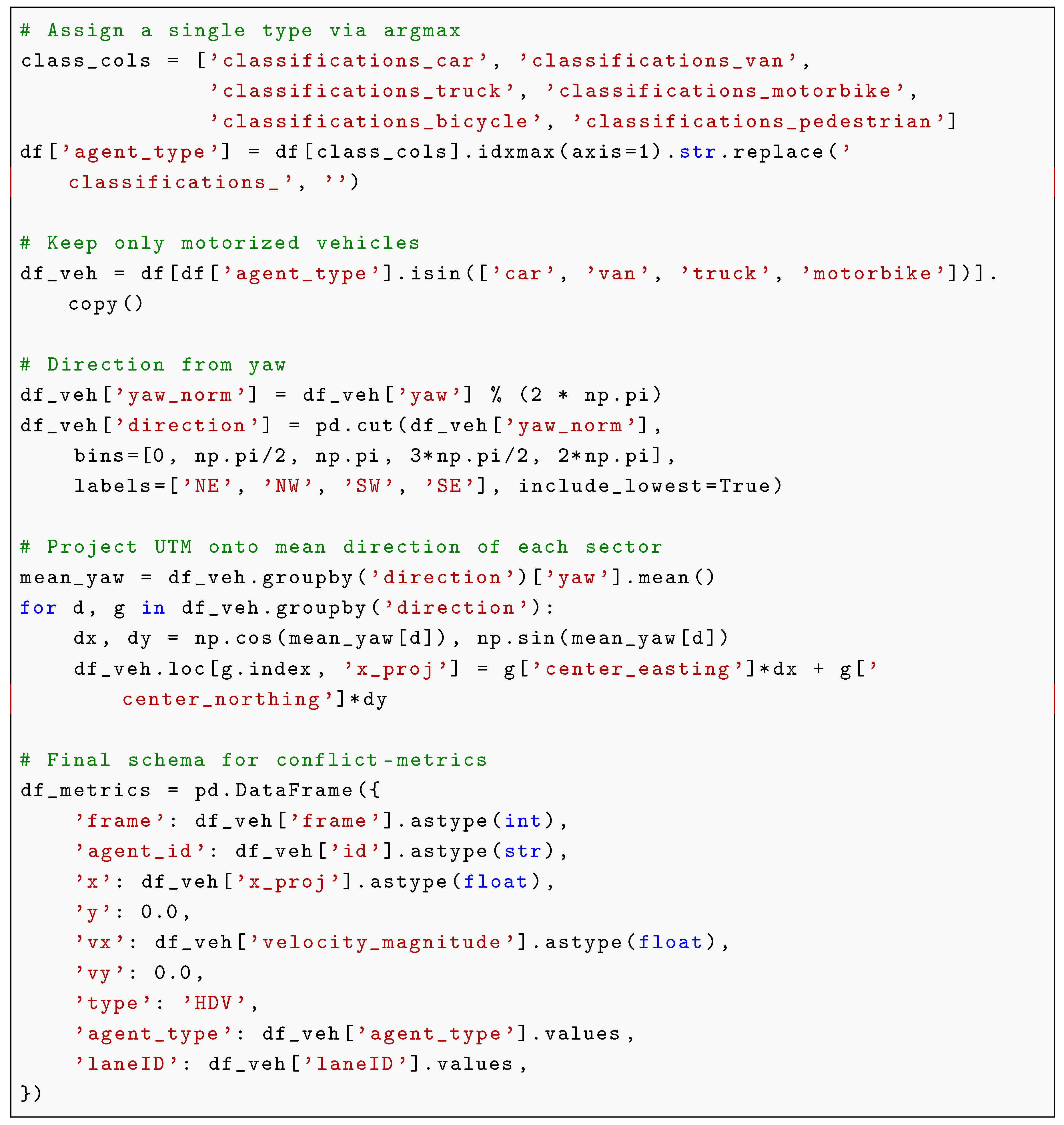 |
The type column is set to ’HDV’ for all objects because the conflict-metrics schema requires it; the model itself does not use this column, and the vehicle class is carried in agent_type.
In this fragment the sector identifier (NE, NW, SW, SE) coincides with the laneID value (lane 1 = NE, lane 2 = NW, lane 3 = SW, lane 4 = SE), so we use “direction (lane k)” as a single label. Within a sector there may be 2–3 physical lanes, so the quantities reported below are sector-level, not lane-level.
4. Conflict Metrics
The conflict metrics follow the two-layer model of [1]. Layer 1 is environment-specific: it contains the movement models and the micro-level metrics that reflect the physics of a given environment. For road traffic these are car-following models and the surrogate safety measures (TTC, DRAC). Layer 2 is universal: it defines a three-level system of metrics and the state parameters derived from it, and it is independent of the environment. The present section restates Layer 2 in the notation of [1]; the urban-specific part (Layer 1) is described in Section 3.
4.1. State of a Leader–Follower Pair
The state of a leader–follower pair at time t is given by , where s is the gap and is the relative speed, with . Two boundaries are introduced:
A frame is conflicting if both conditions hold: and .
The pair type P is determined by the nature of the leader and the follower. In this work, P is a vehicle-class combination such as , , or . Layer 2 does not depend on the specific set of types, and the basic aggregation inequality below holds for any finite set of types.
4.2. Three-Level Metrics
The three levels take the form:
Here is the number of pairs of type P, and are the numbers of conflicting and total frames of the i-th pair, N is the total number of frames, is the number of frames in which at least one pair of type P is in conflict, and is the number of frames in which at least one pair of any type is in conflict.
Basic aggregation inequality.
The levels are related by
Proof sketch. The lower bound follows because every conflicting frame contains at least one pair type, so the set of conflicting frames is the union of the per-type sets; the upper bound follows from subadditivity of the union. The lower bound is attained when all conflicts belong to a single type; the upper bound is loose when types co-occur in the same frame. The inequality is also checked computationally on the DLR UT data; see Table 3 and Section 6.
4.3. State Parameters
From the meso-level metrics, two state parameters are introduced:
Here M is the limiting conflict (the contribution of the dominant pair type) and is the boundary gap (structural heterogeneity). The pair forms a two-dimensional coordinate of the meso-level distribution: M measures dominance (how much one pair type prevails), and measures excess (how much the other types add to the sum ). Although is computed from M and S, the two parameters are not equivalent: for a fixed M, an increase in means that conflict is distributed among several types rather than concentrated in one. The pair is precisely the diagnosis of the stream structure: it tells which groups of agents shape the macro-state, and therefore which control action is appropriate. The integral distance to the target state is
The control objective for conflict is , which is equivalent to .
Position of C within the inequality band.
By (5), C lies between M and . The position of C within this band is informative. If , the conflicting frames of different pair types are almost disjoint: each frame is dominated by a single type, and the types behave as separate risk channels. If , the conflicting frames of different pair types overlap: several types are in conflict in the same frame, and the types co-occur rather than replace each other. The normalized position
therefore measures the co-occurrence of pair types within conflicting frames: means separation, means co-occurrence. For the DLR UT data is reported in Table 3.
4.4. Calibration of the TTC Threshold
The TTC threshold is calibrated per lane on the longest continuous interval in which every frame contains at least three vehicles; the 5th percentile of the empirical TTC distribution over active pairs within this interval is used as the threshold. This adapts the threshold to the traffic phase and preserves discriminative power at different densities. The DRAC threshold is fixed at m/s2. An active pair is a pair of adjacent vehicles in the same lane (ordered by longitudinal position) with and m. This calibration procedure is the same as in [1] and in the analyze_frenet.py script of the conflict-metrics library [2].
4.5. Transfer to an Urban Environment
Layer 2 is environment-invariant by construction: its metrics (, , C, M, , r, ) are defined only through the observable quantities and and contain no parameters that depend on the environment. Applying the model to the DLR UT dataset therefore requires only instantiating Layer 1 with the urban preprocessing described in Section 3: classification of agents, filtering of pedestrians and bicycles, assignment of a direction label, projection of the UTM coordinates onto the mean direction of each sector, and formation of leader–follower pairs. The metrics and the aggregation inequality (5) themselves are unchanged; this is the sense in which the two-layer model is universal across the highway case (UTE) of [1] and the urban case (DLR UT) of the present paper.
5. Results: Dominant Pair Types and Per-Type Contribution
Table 1 combines the frequency of dominant pair types, the number of records in which each type occurs, and the mean for each type across all 372 records. Combining the three columns makes the table informative: it shows which types dominate both by frequency and by per-pair contribution.
Interpretation. car→car gives both the largest absolute contribution (, i.e., ) and the largest per-pair contribution: its is an order of magnitude higher than that of any other pair type (). Among the non-car types, car→truck has the highest per-pair (), followed by truck→truck () and motorbike→car (). This indicates that, while car→car pairs dominate the aggregate conflict load, heavy-vehicle interactions (car→truck, truck→truck, truck→car) form a distinct secondary risk cluster that deserves separate attention in safety analysis.
Table 2 complements this aggregate view with a per-encounter breakdown by vehicle type. The top section reports aggressive followers (those with in at least one interval), the bottom section reports leader magnets (top-10 by in each interval), both aggregated over all 96 intervals. Car followers dominate by count (600 of 647), but per encounter van followers show a comparable mean ( vs. for car) at a higher mean ( vs. m/s). Truck followers are the least aggressive per encounter (, m/s, gap m), consistent with their larger mass and longer braking distances. Among leader magnets, motorbike leaders show the highest per-encounter ( vs. for car), despite being the rarest type (16 appearances); they are also the slowest on average ( km/h vs. km/h for car), which is exactly the “slow leader” scenario. These per-encounter numbers should be read with caution: the samples for van, truck, and motorbike are small (13–69 appearances), the 95% bootstrap confidence intervals in Table 2 overlap for all non-car types, and a single interval can dominate the mean. They are indicative, not conclusive.
6. Results: Vs and the Diagnosis
Table 3 compares (share of conflict frames over all frames) and (median over 10-second windows), averaged over the day, and reports the state parameters M, , r and the co-occurrence index for each direction.

Table 3.
Comparison of and , and state parameters by direction (mean over the day, 372 records).
| Direction | M | r | ||||||
|---|---|---|---|---|---|---|---|---|
| NE (1) | 0.0482 | 0.0141 | 0.0484 | 0.0696 | 0.0429 | 0.0060 | 0.0435 | 0.88 |
| NW (2) | 0.0421 | 0.0116 | 0.0423 | 0.0674 | 0.0373 | 0.0053 | 0.0380 | 0.91 |
| SW (3) | 0.0447 | 0.0088 | 0.0452 | 0.0690 | 0.0376 | 0.0077 | 0.0391 | 0.92 |
| SE (4) | 0.0213 | 0.0024 | 0.0213 | 0.0378 | 0.0184 | 0.0030 | 0.0189 | 0.97 |
Burstiness. and agree to within percentage points for all directions, while is systematically lower, by – percentage points. This is the signature of bursty conflict: most 10-second windows contain no conflicts, but the windows that do contain conflicts are intense. The effect is strongest for NE ( vs. ) and weakest for SE ( vs. ). This matches the highway case (UTE) of [1] and is reported here as a consistency check, not as a separate contribution.
Structure of conflict via and . The ratio is approximately 7 in all four directions (NE: ; NW: ; SW: ; SE: ), and the co-occurrence index is close to the right edge of the inequality band in all four directions (, , , for NE, NW, SW, SE respectively). Two conclusions follow.
First, the structural composition of conflict does not change across directions: in every direction a single pair type (car→car) dominates the meso-level distribution, and is small relative to M. What changes across directions is only the intensity r: NE is the most conflict-prone (), SE the least (), and NW and SW are intermediate. This is exactly what the diagnosis is designed to reveal: the macro-state differs across directions mainly in magnitude, not in composition.
Second, C sits near the right edge of the inequality band, not near the left edge. Since means that the conflicting frames of different pair types overlap, the values – mean that different pair types co-occur in the same conflicting frames rather than replacing each other: when the stream is in conflict, it is usually in conflict for several pair types at once, not for one type at a time. This is the expected behaviour in a dense urban intersection, where a single leader can simultaneously be in conflict with a following car and with a following truck, and a single frame can contain several conflicting pairs of different types. The near-right-edge position of C is therefore not a numerical curiosity: it is a structural property of the urban stream, and it is why the upper bound of (5) is loose (the sum counts the same frame several times). In the highway stream of [1], by contrast, the stream is HDV-only and all pairs have the same type, so the question of co-occurrence does not arise and by construction.
Figure 1 shows the daily dynamics of C for each direction. Figure 2 visualises the inequality check for the NE direction: the red line (C) stays within the grey band () and close to its upper edge, confirming the fundamental inequality on real data and the co-occurrence of pair types. The same inequality holds for all four directions (see Table 3). Figure 3 shows the relationship between C and traffic volume.
7. Danger Report Example
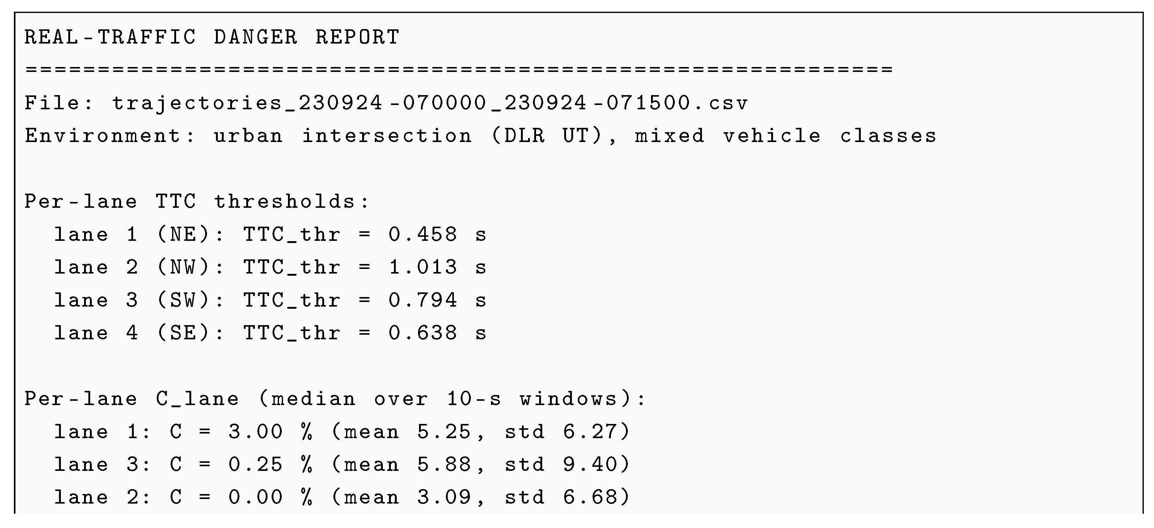
The danger_report script was introduced in [1] for the UTE highway stream, where it reported per-lane thresholds, hot lanes, aggressive followers, leader attractors, and top pairs by . We reuse the same script from the dlr-ut-conflict-metrics repository [3] (which depends on conflict-metrics [2]) and instantiate it for an urban, mixed-class interval. The format of the report is unchanged; the only extension is that every follower, leader, and pair now carries a vehicle-class label (car, van, truck, motorbike) and every lane index is annotated with a direction label (NE, NW, SW, SE). This extension is not a contribution in itself — it is what makes the report directly usable for urban control actions (e.g., warn a truck follower approaching a slow motorbike leader in the NE sector) rather than only for highway lane management. This section illustrates the tool on a single interval; it is not a separate result.
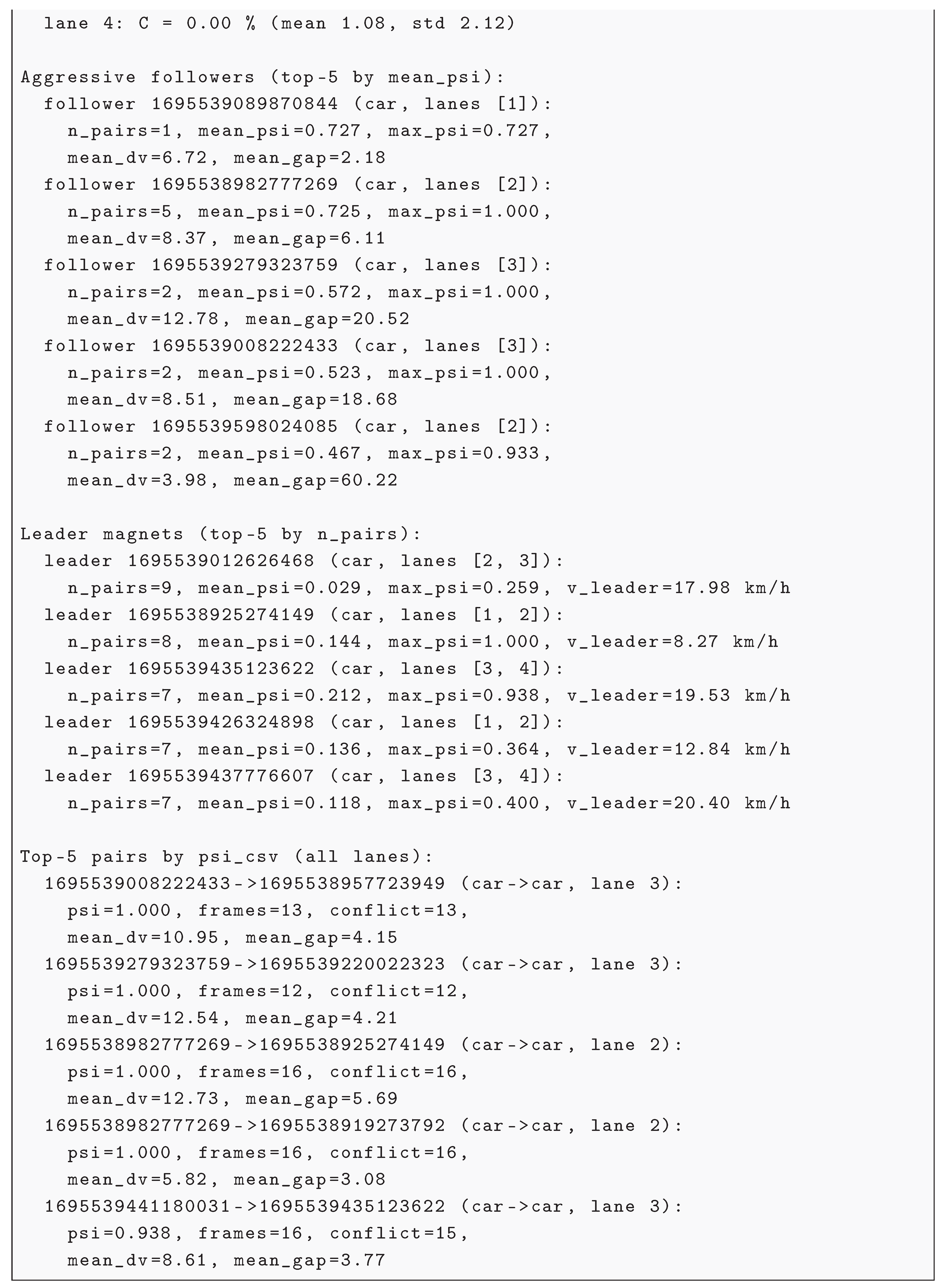
Below is an example output for the morning-peak interval 07:00–07:15 UTC (file trajectories_230924-070000_230924-071500.csv). This interval was chosen because it contains the most conflicting pairs of the day ( for several pairs), in contrast to the night-time interval 00:00–00:15, where conflict is sparse.
| Listing 2. Danger report for the 07:00–07:15 morning-peak interval (abridged; top-5 aggressive followers and top-5 leader magnets are shown). The format is the same as in [1]; the vehicle-class and direction labels are the urban instantiation. |
|
7.1. Aggregation Across Frames
The most conflicting pairs have very small gaps (e.g., 1.97–3.32 m for the top pairs in lanes 2–3) combined with high relative speeds (up to 12.78 m/s). This is exactly the pattern that the two-layer model is designed to detect: a high and a small gap produce a low TTC and a high DRAC simultaneously, so the pair is flagged as conflicting in most frames (). Urban encounters are short ( for most top pairs), so on 12 frames is much noisier than on the 47+ frames required in the highway case of [1]. The urban report therefore prints frames next to every pair, and we recommend reading together with rather than in isolation.
7.2. Aggregation Across Pairs
One follower requires separate evaluation. Follower 1695539598024085 (car, lane 2) has both a high conflict index (, ) and a large mean gap ( m) at a moderate mean relative speed ( m/s). This combination may look paradoxical at first sight, but it is not. In this interval the follower has pairs, both of type car→car:
- pair : , mean gap m, mean m/s, mean TTC s. Frame by frame, the gap shrinks from m to m, TTC drops to s, and DRAC rises to m/s2; 14 of 15 frames are conflicting;
- pair : , mean gap m, mean m/s, mean TTC s (a far-away vehicle ahead, never in conflict).
The reported per-follower mean gap ( m) is the average of the two pair-level mean gaps; it is large not because the follower keeps a large gap, but because one of its two pairs is far away. The same composition effect inflates the mean ( m/s on average, m/s for the conflicting pair) and deflates the mean ( on average, for the conflicting pair). This is a second, distinct aggregation pitfall: aggregation across pairs, not only across frames. A per-follower mean over a small number of pairs ( here) is dominated by the pair composition, and the same follower can appear as a top aggressive follower or as a safe follower depending on which pairs happen to be built in a given interval. Such followers should be inspected pair by pair before any control action is derived from them; a high per-follower is a diagnostic signal, not a verdict. In the highway stream of [1] a follower typically accumulates many pairs within a lane over the 5.5-min segment, so this composition effect is averaged out; in the urban case it is not, and the per-follower mean must be read together with .
7.3. Leader Magnets
The report also identifies leader magnets: leaders that attract a large number of conflicting followers. Leader 1695539012626468 has the most followers () but a low mean : it is often followed, but rarely in conflict. In contrast, leader 1695538925274149 has 8 followers, mean , and maximum : it is slow (mean speed 8.27 km/h), and at least one follower that approaches it enters a conflict in every frame. This is the “slow leader” scenario already discussed in [1]: a slow leader creates a high for the follower, which drives the conflict index up.
The most extreme case in the full day is a motorbike leader (ID 1695584982736428, lane 1) that is almost stationary ( km/h): with and , every follower that approaches it enters a conflict. This is the “slow leader” scenario in its purest form. It also illustrates why the leader type matters: the motorbike group has the highest per-encounter mean among leader magnets in Table 2b ( vs. for car), but the 95% bootstrap CI for the motorbike group is wide () and overlaps with the car group, so this ordering is indicative rather than conclusive. The extreme case itself (a stationary motorbike leader) is a fact, not a statistical estimate. The highway stream of [1] contained no motorbikes, so this slow-motorbike-leader scenario could not be observed there; it is a property of the DLR UT mixed vehicle classes, not of the report format.
Practical recommendations (urban).
(i) Warn car followers with and m/s in the NE sector. (ii) Warn followers approaching slow motorbike leaders (the extreme case is ID 1695584982736428, km/h). (iii) Monitor lane 1 (NE) as the hot direction. (iv) Use “slow motorbike leader / high- car follower” as an urban ADAS/V2X test case — this scenario is absent from the highway UTE stream.
8. Discussion
- What the metrics show.
The three-level system and the state parameters provide not merely “how many conflicts” but where exactly they are concentrated and how they are structured. On the DLR UT data, two things are visible. First, in all directions, so the composition of conflict (car→car dominance) is stable and only the intensity r changes. Second, is close to the right edge of the inequality band (–), which means that different pair types co-occur in the same conflicting frames rather than replacing each other; this is the structural reason why the upper bound of the aggregation inequality is loose in the urban case. are geometric coordinates of the meso-level distribution, not information-theoretic measures of synergy; their interpretation is limited to the state-space geometry described in Section 4.
- What the danger report shows.
The danger_report exposes two aggregation pitfalls that do not arise in the HDV-only highway case: short encounters inflate the noise of when is small, and small make the per-follower mean dominated by pair composition. Both pitfalls are properties of the urban data, not of the script, and both are diagnostic signals that should be inspected before any control action is derived.
- Validation on real trajectories.
The present work validates on real DLR UT trajectories rather than on simulation alone. This is a deliberate choice: Qu and Wu [8] show that the correlation between simulated SSMs and field-observed conflicts is not stable across thresholds and that public data are often insufficient for a robust link between simulated SSMs and real crashes. Real-trajectory validation avoids this particular pitfall, although it introduces the data-volume limitations listed in Section 9.
- Practical implications.
Urban conflict management at this intersection should focus on car→car pairs in the NE sector, where both the intensity r and the dominant contribution M are highest, and slow motorbike leaders are a distinct test case for ADAS/V2X that is absent from highway data. The near-right-edge position of C also implies that warning systems should not treat pair types independently: when the stream is in conflict, several types are usually in conflict at once.
9. Limitations
- Data volume. The public fragment covers one day (24 September 2023), and within it the per-type samples are small: among the 647 aggressive followers, 600 are cars, and van, truck, and motorbike together account for 47 appearances (Table 2a); motorbike leaders account for only 16 appearances (Table 2b). The absolute values reported here (e.g., for NE, and the per-encounter for non-car types) are therefore illustrative of this day and indicative rather than conclusive. Confirmation requires a multi-day, multi-intersection record.
- Direction as a proxy for lane. The sector label (NE, NW, SW, SE) coincides with the laneID in this fragment, but within a sector there may be 2–3 physical lanes. The reported quantities are therefore sector-level, not lane-level, and cannot be used to rank individual lanes within a sector.
- Aggregation across pairs. For followers with a small number of pairs (), the reported per-follower mean gap, mean , and mean are dominated by the pair composition rather than by the follower’s behaviour; the case of follower 1695539598024085 (Section 7.2) is a direct illustration. A high per-follower should therefore be inspected pair by pair before any control action is derived from it.
10. Conclusions
The two-layer conflict model was applied to the DLR UT dataset (urban intersection with mixed vehicle classes). The results on this single day show that:
- 1.
- car→car dominates both by absolute contribution and per pair ( vs. for all other types); among non-car types, car→truck has the highest per-pair (), followed by truck→truck ().
- 2.
- The NE direction is the most conflict-prone (), consistent with the LTWO scenario; the SE direction is the least conflict-prone ().
- 3.
- The structural composition of conflict is stable across directions: in all four directions, and the co-occurrence index is close to the right edge of the inequality band (–), meaning that different pair types co-occur in the same conflicting frames rather than replacing each other. Only the intensity r changes across directions.
- 4.
- Conflict is bursty: by – percentage points across all directions, as in the highway case (UTE).
- 5.
- Per-encounter, van followers show a mean comparable to car and motorbike leaders show the highest mean among leader magnets; these effects are based on small samples (13–16 appearances) and wide bootstrap confidence intervals, and are indicative rather than conclusive.
These findings confirm the universality of Layer 2 (the conflict model) across different environments (highway vs. urban intersection) and different pair types. The danger_report of [1] transfers to the urban mixed-class case without changes to its format; the urban instantiation adds vehicle-class and direction labels and is used to illustrate two aggregation pitfalls specific to short urban encounters. For practice, urban conflict management at this intersection should focus on car→car pairs in the NE sector, and slow motorbike leaders are a distinct test case for ADAS/V2X that is absent from highway data.
Author Contributions
A.V. Chernyshov: conceptualization, methodology, software, validation, formal analysis, writing – original draft. The author bears sole responsibility for the content of the work.
Funding
This research received no external funding.
Institutional Review Board Statement
Not applicable.
Informed Consent Statement
Not applicable.
Data Availability Statement
The DLR Urban Traffic (DLR UT) dataset analysed in this study is publicly available from the DLR Institute of Transportation Systems; the public fragment covering 24 September 2023 is the one used here. The UTE dataset referenced for comparison is available at SEU Traffic (http://seutraffic.com). The conflict-metrics library (model, metrics, calibration, and danger_report) is available at https://github.com/andreychernyshov5-beep/conflict-metrics. The urban preprocessing, the DLR UT adapter, and the scripts reproducing the results of this paper are available at https://github.com/andreychernyshov5-beep/dlr-ut-conflict-metrics.
Acknowledgments
The author thanks the developers of the DLR UT dataset for making the data available.
Conflicts of Interest
The author declares no competing interests.
Abbreviations
The following abbreviations are used in this manuscript:
| SSM | Surrogate Safety Measure |
| TTC | Time-to-Collision |
| MTTC | Modified Time-to-Collision |
| DRAC | Deceleration Rate to Avoid a Crash |
| PICUD | Potential Index of Crash Under Deceleration |
| Weighted Combination of Spacing and Speed Difference Rates | |
| HDV | Human-Driven Vehicle |
| CAV | Connected and Automated Vehicle |
| DLR UT | DLR Urban Traffic dataset |
| UTE | Ubiquitous Traffic Eyes dataset |
| LTWO | Left Turn With Oncoming traffic |
References
- A.V. Chernyshov. Conflict metrics for traffic streams: a two-layer model with a micro-macro link. Preprints 2026, 202611.0404. [CrossRef]
- A.V. Chernyshov. conflict-metrics: Conflict metrics for traffic streams. GitHub repository, v1.0, 2026. https://github.com/andreychernyshov5-beep/conflict-metrics.
- A.V. Chernyshov. dlr-ut-conflict-metrics: Urban and mixed-traffic extension of the two-layer conflict model (DLR UT dataset). GitHub repository, 2026. https://github.com/andreychernyshov5-beep/dlr-ut-conflict-metrics.
- C. Schicktanz, L. Klitzke, K. Gimm, S. Knake-Langhorst, G. Rizzo, H.H. Mosebach, K. Liesen. The DLR Urban Traffic Dataset (DLR-UT): A Comprehensive Traffic Dataset from an Urban Research Intersection. In 2025 IEEE Intelligent Vehicles Symposium (IV), pp. 398–405, 2025.
- C. Schicktanz, K. Gimm. Detection and analysis of corner case scenarios at a signalized urban intersection. Accident Analysis and Prevention, vol. 210, p. 107838, 2025.
- M. Zhang, J. Yang, X. Yang, X. Duan. Measuring collision risk in mixed traffic flow under the car-following and lane-changing behavior. Applied Sciences, vol. 14, no. 23, p. 11400, 2024. [CrossRef]
- A. Singh, S. Dass. A PRISMA review of the use of surrogate safety measures at signalized intersections with a focus on its application in mixed traffic condition. Innovative Infrastructure Solutions, vol. 10, no. 6, pp. 227.1–227.19, 2025. [CrossRef]
- A. Qu, C. Wu. Revisiting the correlation between simulated and field-observed conflicts using large-scale traffic reconstruction. Accident Analysis and Prevention, vol. 210, p. 107808, 2025. [CrossRef]
- J.C. Hayward. Near Miss Determination through Use of a Scale of Danger. Highway Research Board, Washington, DC, USA, 1972.
- K. Ozbay, H. Yang, B. Bartin, S. Mudigonda. Derivation and validation of new simulation-based surrogate safety measure. Transportation Research Record, vol. 2083, pp. 105–113, 2008.
- N. Uno, Y. Iida, S. Itsubo, S. Yasuhara. A microscopic analysis of traffic conflict caused by lane-changing vehicle at weaving section. In Proceedings of the 13th Mini-EURO Conference, Bari, Italy, 2002, pp. 10–13.
- K. Hou, F. Zheng, X. Liu. Enhancing mixed traffic safety assessment: A novel safety metric combined with a comprehensive behavioral modeling framework. Accident Analysis and Prevention, vol. 208, p. 107766, 2024.
Figure 1.
Share of conflict frames C by direction over 24 September 2023. The NE direction (top-left) shows the highest peaks, consistent with the LTWO scenario.
Figure 1.
Share of conflict frames C by direction over 24 September 2023. The NE direction (top-left) shows the highest peaks, consistent with the LTWO scenario.
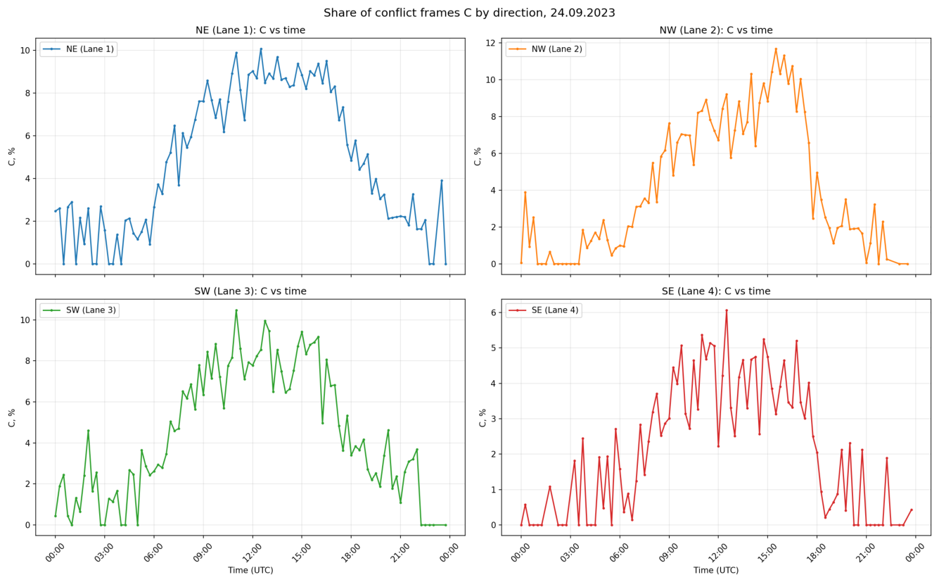
Figure 2.
Inequality check for the NE direction (Lane 1). The red line (C) stays within the grey band () and close to its upper edge (), confirming the fundamental inequality on real data and the co-occurrence of pair types within conflicting frames.
Figure 2.
Inequality check for the NE direction (Lane 1). The red line (C) stays within the grey band () and close to its upper edge (), confirming the fundamental inequality on real data and the co-occurrence of pair types within conflicting frames.
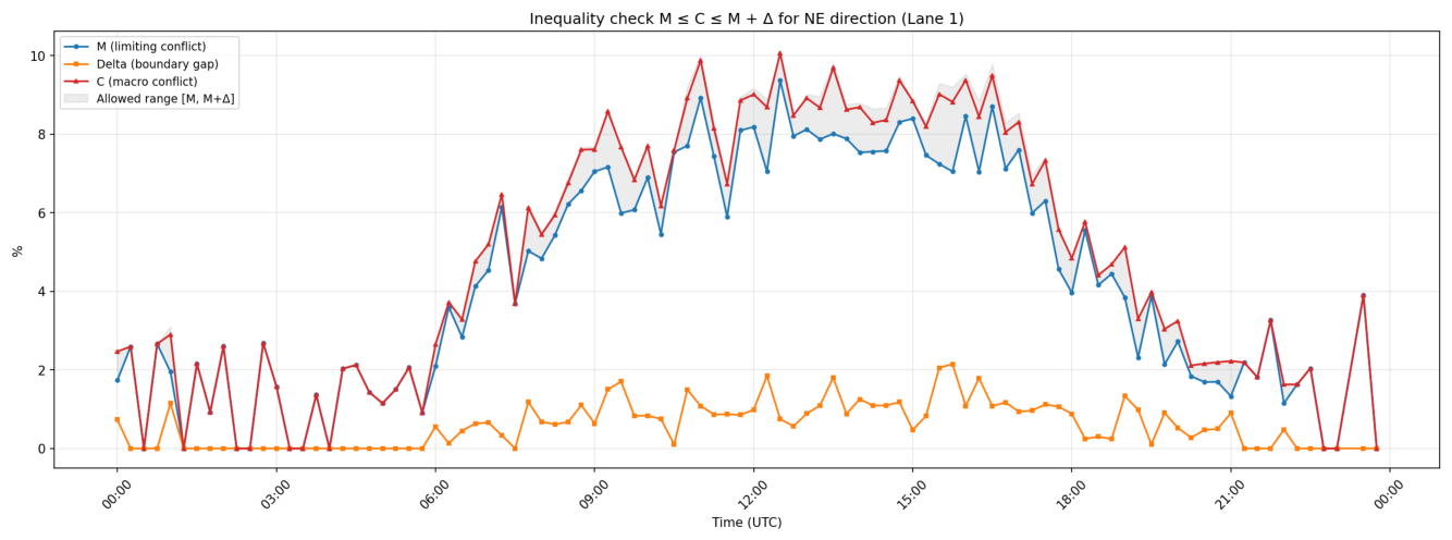
Figure 3.
Conflict share C versus traffic volume (number of vehicles per 15-min interval) by direction.
Figure 3.
Conflict share C versus traffic volume (number of vehicles per 15-min interval) by direction.
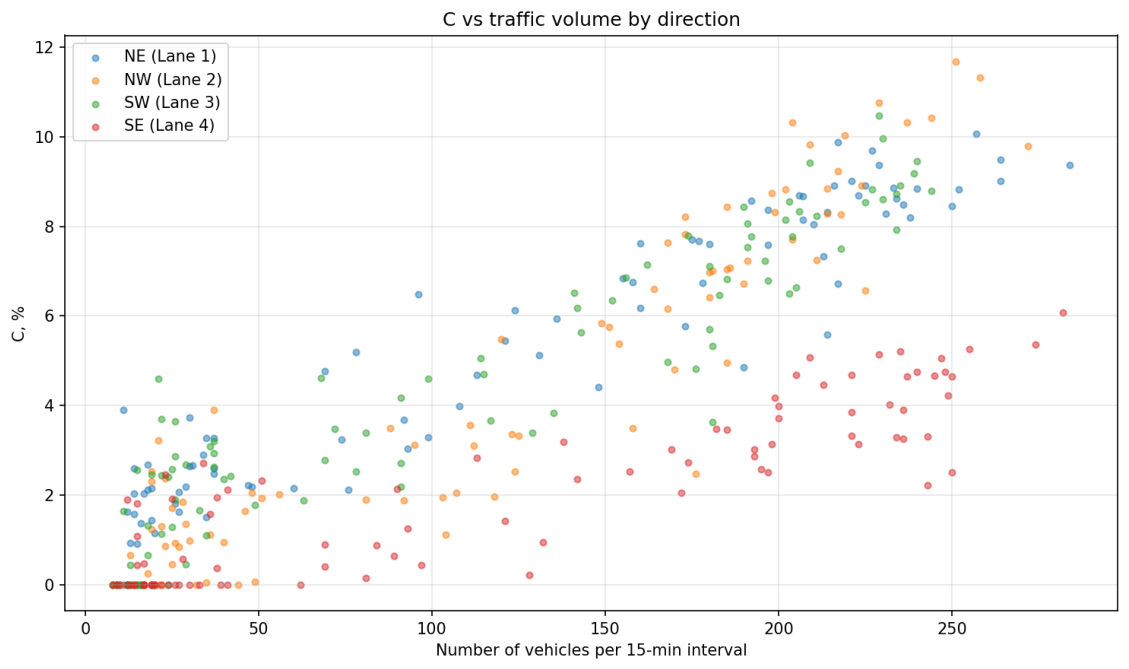
Table 1.
Pair-type summary across all 372 records: number of records in which the type is dominant, number of records in which it occurs, and mean . Only pair types with at least one occurrence are shown.
Table 1.
Pair-type summary across all 372 records: number of records in which the type is dominant, number of records in which it occurs, and mean . Only pair types with at least one occurrence are shown.
| Pair type | Mean | ||
|---|---|---|---|
| car→car | 337 | 298 | 0.0416 |
| car→truck | 10 | 149 | 0.0037 |
| truck→truck | 5 | 14 | 0.0033 |
| truck→car | 7 | 127 | 0.0025 |
| motorbike→car | 4 | 160 | 0.0027 |
| car→van | 4 | 132 | 0.0026 |
| car→motorbike | 3 | 152 | 0.0024 |
| van→car | 1 | 120 | 0.0020 |
| truck→motorbike | 0 | 8 | 0.0013 |
| motorbike→motorbike | 0 | 16 | 0.0009 |
| motorbike→van | 0 | 17 | 0.0008 |
| truck→van | 0 | 10 | 0.0008 |
| motorbike→truck | 1 | 17 | 0.0007 |
| van→truck | 0 | 6 | 0.0007 |
| van→van | 0 | 13 | 0.0005 |
| van→motorbike | 0 | 9 | 0.0004 |
Table 2.
Per-encounter statistics by vehicle type, aggregated over all 96 intervals. Top: aggressive followers (mean in at least one interval). Bottom: leader magnets (top-10 by in each interval). “Appearances” is the number of (interval, vehicle) records, not unique vehicles across the day. The 95% CI for mean is obtained by bootstrap over appearances; the column replaces the uninformative maximum (which is for all types).
Table 2.
Per-encounter statistics by vehicle type, aggregated over all 96 intervals. Top: aggressive followers (mean in at least one interval). Bottom: leader magnets (top-10 by in each interval). “Appearances” is the number of (interval, vehicle) records, not unique vehicles across the day. The 95% CI for mean is obtained by bootstrap over appearances; the column replaces the uninformative maximum (which is for all types).
| Vehicle type | Appearances | Mean | 95% CI | Mean , m/s | |
| (a) Aggressive followers | |||||
| car | 600 | 0.449 | [0.42, 0.48] | 0.92 | 8.03 |
| van | 13 | 0.456 | [0.30, 0.61] | 0.85 | 9.45 |
| motorbike | 13 | 0.406 | [0.24, 0.57] | 0.84 | 8.52 |
| truck | 21 | 0.327 | [0.20, 0.46] | 0.71 | 6.61 |
| (b) Leader magnets | |||||
| Vehicle type | Appearances | Mean | 95% CI | Mean | |
| car | 811 | 0.110 | [0.09, 0.13] | 0.50 | 7.58 |
| motorbike | 16 | 0.222 | [0.10, 0.35] | 0.62 | 4.44 |
| van | 31 | 0.121 | [0.07, 0.17] | 0.45 | 7.36 |
| truck | 69 | 0.099 | [0.07, 0.13] | 0.42 | 5.29 |
Disclaimer/Publisher’s Note: The statements, opinions and data contained in all publications are solely those of the individual author(s) and contributor(s) and not of MDPI and/or the editor(s). MDPI and/or the editor(s) disclaim responsibility for any injury to people or property resulting from any ideas, methods, instructions or products referred to in the content. |
© 2026 by the authors. Licensee MDPI, Basel, Switzerland. This article is an open access article distributed under the terms and conditions of the Creative Commons Attribution (CC BY) license (http://creativecommons.org/licenses/by/4.0/).
Copyright: This open access article is published under a Creative Commons CC BY 4.0 license, which permit the free download, distribution, and reuse, provided that the author and preprint are cited in any reuse.