

Submitted:
08 November 2026
Posted:
10 November 2026
You are already at the latest version
Abstract
This is the third paper of a series on Four Null Spacetime Theory, in which spacetime is built from finite cells spanned by four lightlike vectors in perfect balance. The first two papers established the geometry of one cell and how cells meet; this one asks how radiation and gravity act on them. On a light front gravity separates by spin into the Raychaudhuri and Damour constraints and two radiative polarizations, and the cell preserves the separation: its scalar sector has only a double root, its vector sector a positive dressing, and its finite step corrections have unique covariant forms. Symmetry and locality alone do not fix the finite cell law, as explicit counterexamples show; causality does, given one premise, that the law’s principal part depends on the reconstructed metric alone and not on the cell’s clock; observation bounds the speed difference such a coupling would produce at long wavelengths to about one part in 1015, but does not establish that the coupling vanishes. For a reversible two step law whose kernel stays within its causal reach and which is stable at every momentum, Bernstein’s inequality bounds every propagation speed by the reach, and equality forces Kirchhoff’s law on the sphere one cell away, with quartic coefficient one twelfth; the shell family that earlier work left open reaches beyond the light cone and is excluded, and scale invariance under blocking independently selects the same law. On the Regge lattice of the cell the Fierz Pauli graviton appears with the correct normalization. Requiring the propagation law on curved backgrounds to come from one action fixes the Einstein coupling to one and, through order of the cell size squared in the transverse traceless sector, a unique completion whose coefficients are exact rationals, with the extrinsic coefficient two thirds, all certified in exact a rithmetic. The constraints remain first class, their lattice forms are preserved to fourth order along rays, and the ray network radiates by the quadrupole formula. Every result is stated with its status, and every verified result is reproduced by the archived package.
Keywords:
general relativity
; gravitational waves
; discrete spacetime
; Regge calculus
; Huygens principle
; Kirchhoff’s formula
; characteristic evolution
; null hypersurfaces
; Raychaudhuri equation
; Damour equation
; Linearized gravity
; Fierz–Pauli theory
; graviton interactions
; transverse-traceless perturbations
; quadrupole radiation
; effective field theory of gravity
; emergent spacetime
; Fierz–Pauli action
; Huygens principle
; Four Null Spacetime Theory
What This Paper Achieves
The central idea of the series. Spacetime is a fabric of finite cells, each spanned by four lightlike vectors in perfect balance, and that balance, not any added structure, is what organizes geometry, curvature, propagation and fields. The local idea of this paper. On balanced cells radiation advances by one exact law, Kirchhoff’s law on the sphere one cell away, selected by causality rather than chosen, given a principal part free of the cell’s clock, and gravity follows from it: the constraints keep only the two polarizations of general relativity, and requiring one action fixes the Einstein interaction and its cell scale completion as exact rational numbers, with no fitted parameter.
| Result | What it establishes | How it supports the central idea |
| Gravity on a light front (Section 2) | constraints and two radiative polarizations; the cell’s finite step forms are unique and add no mode | the cell carries exactly the degrees of freedom of general relativity |
| Why geometry alone does not fix the law (Section 3) | explicit stable, isotropic laws with the right cone but the wrong finite cell behavior | identifies the missing principle precisely |
| The Huygens law and its causal selection (Section 4) | given a principal part free of the clock, causality, stability and propagation at the reach force Kirchhoff’s law and equal to one twelfth | the cell’s own light cone selects its propagation law |
| The Regge lattice (Section 5) | the Fierz Pauli graviton with the correct normalization | the cell geometry of Papers I and II carries Einstein gravity |
| Integrability (Section 6) | the Einstein coupling and a unique completion in exact rationals, with x equal to two thirds | gravity’s interaction follows from propagation, with nothing fitted |
| Beyond the transverse traceless sector (Section 7) | four further coefficients conditionally fixed; one direction isolated | locates precisely what dynamics must still supply |
| Consistency of the constraints (Section 8) | first class constraints, lattice forms preserved to fourth order, a safe near resonant channel | the cell’s dynamics keeps general relativity’s structure |
| Radiation and the weak field (Section 9) | the quadrupole formula; corrections that are contact terms; the classical tests | the cell reproduces the observed gravitational physics |
Place in the series. This paper builds on Four Null Spacetime Theory I. The Balanced Null Cell: from the Regular Tetrahedron to the Metric, the Hodge Split, the Relational Clock and Spinors [16] and Four Null Spacetime Theory II. Transport, Gluing and Discrete Curvature: Shared Faces, Holonomy, Spin Structures and Closed Balanced Spacetimes [17], cited below as Papers I and II. Paper I supplies the cell, its clock and the subdivision into 24 simplices used here as a Regge lattice; Paper II supplies the transport between cells and the open question, from its Route B, of the one interaction coefficient this paper isolates. The series continues with IV. Fields on the Four Null Fabric, V. Characteristic Dynamics of Free Gravity and VI. Quantum Geometry of Four Null Cells.
Postulates used. Of the six postulates of the theory, listed in Paper I, this paper uses null canonical primacy, balance and the composite clock, which the gauge consistency tests require to transform with the generators; it derives the Huygens law of the third postulate within a stated class of laws, under the premise that the generators are characteristics of the propagation law, the dynamical form of null canonical primacy, confirms it by the blocking of the fifth, and uses the integrability of the sixth.
Status and AI disclosure. Exact means proved symbolically or in exact arithmetic, and machine checked; certified means supported as a polynomial identity by randomized exact arithmetic tests, with the stated false acceptance probability; verified means checked numerically; conditional marks a result that holds under a stated assumption; cited marks a result from an earlier record of the program that is not rerun in this paper’s package; reported marks a possibility computed in the program but neither proved nor reproducible here, stated for completeness and never used as a premise; open marks what is not settled. The calculations were carried out with AI assistance under the author’s direction; these are internal checks, not external replication.
1. Introduction
- In Brief: what a propagation law and an interaction must satisfy
Papers I and II built the cell and the fabric: four balanced lightlike generators, their metric and clock, and the transport between cells that share a face. This paper asks how radiation and gravity act on them. Three things must be settled. First, which parts of gravity propagate and which are constraints; on a light front general relativity answers this by spin, and the cell must preserve the answer. Second, the propagation law itself: every candidate must reproduce the light cone at long wavelengths, but the finite cell behavior can differ, and something must select it. Third, the interaction: once a law is fixed on flat space, its form on curved space determines how gravitational waves interact, and the question is whether anything fixes that form.
Formulation A. The program calls its present architecture Formulation A. It keeps the four tetrahedral null directions of Paper I as the smallest local causal seed, carries free fields with a Huygens law, imposes the null constraints on each ray, and evolves along null rays rather than on spacelike slices. It was introduced to replace an earlier rigid update on spacelike slices, which grows at the cell scale, as Paper V shows. The propagation law and the interaction derived in this paper are those of the Formulation A graviton in the program’s records; Paper V tests the evolution in time.
The results sit on a chain that starts from the geometry of Papers I and II:
Symbols. each arrow marks a step that uses only what precedes it.
The structures of general relativity that must be recovered are retained as requirements at long wavelengths:
| Element | Requirement of general relativity | Realization on the cells |
| Gravitational waves | two tensor polarizations | two transverse shear polarizations |
| Long wavelength propagation | the Einstein wave equation | the Huygens law reduces to it |
| Scalar and vector gravity | constrained, not radiative | Raychaudhuri and Damour constraints |
| Gauge structure | consistency with diffeomorphisms | relational clock and null constraint algebra; Ward identity |
| Transverse traceless interaction through order | the Einstein interaction | fixed by integrability within the stated basis |
The answers come in order. Section 2 separates gravity on a light front and gives the cell’s finite step constraints. Section 3 shows by counterexamples that symmetry and locality do not select the law, and Section 4 shows that causality does, with Kirchhoff’s law as the unique member. Section 5 places Regge calculus on the cell’s subdivision and recovers the Fierz Pauli graviton. Section 6 and Section 7 derive the Einstein interaction and its completion from integrability. Section 8 tests the consistency of the constraints, Section 9 the radiation and the weak field, and Section 10 records where the controlled statements stop.
2. Gravity on a Light Front
- In Brief: gravity has two radiative modes; its other parts are constraints
Finding 1. On a light front gravity separates by spin into constraints and radiation
What we found. On a null surface, made of lightlike rays, the gravitational data separate by spin into three canonical pairs [2,3],
Symbols. is the area density and its conjugate, the spin zero pair; a transverse shift and its momentum, the spin one pair; the shape of the two dimensional cross section and its shear, the spin two pair; A and B label the two transverse directions.
What we found. and only the shear propagates. The spin zero part obeys the Raychaudhuri equation [18,20], and the spin one part the linearized Damour equation [5]:
Symbols. is the expansion of a bundle of rays, its shear and v the parameter along the rays; is the Ricci tensor along the ray direction ℓ, equal to times the matter energy along the ray; marks a small perturbation and V the null coordinate.
What it means. Light bundles focus because of their own convergence, their shear and the matter they cross, and the transverse momentum is fixed by area and shear. These are constraints, not wave equations. The split is a property of Einstein’s equations on null surfaces; it is not assumed here.
What we found. On the cell, a mode changes by a factor per step, and the update obeys a two step recurrence. The constraint forces the scalar update factor to two, and the identity
Symbols. W is the factor by which a mode changes in one step; X is the update factor, equal to W plus its inverse.
What it means. leaves the constrained scalar only the double root at one: the mode never oscillates, so there is no propagating scalar graviton. The cell preserves the split: its finite cell corrections keep the scalar root at one, keep the vector dressing positive (Section 8), and add no mode.
Why it matters. Gravity on the cell has exactly the two polarizations of general relativity.
Scope. Exact in the linear sectors studied.
Finding 2. The finite step constraint has a unique covariant form
What we found. With the square root of the area density, the focusing law along a ray reads
Symbols. a prime is a derivative along the ray; is the squared shear.
What we found. and replacing the second derivative by one centred null step of length gives the finite cell constraint
Symbols. S is the focusing source; the matter energy along the ray; Newton’s constant.
What it means. A centred step differs from the second derivative by one twelfth of the step squared times the fourth derivative, and the focusing law turns that fourth derivative into the bracket. The coefficient is the centred step’s, so no new coefficient appears.
What we found. The constraint uses an affine parameter. For an arbitrary parameter the spin zero connection transforms inhomogeneously, and the correction has a covariant form,
Symbols. f generates an infinitesimal change of the parameter along the ray; is the covariant correction.
What it means. It transforms with weight four and reduces to the bracket above in the affine gauge, where the connection is half the expansion. Within the general local form with these derivative orders and no new field, these two conditions have exactly one solution, so the covariant completion is unique.
Why it matters. The cell’s correction to focusing is fixed completely, by the step and by covariance.
Scope. Exact; the uniqueness is solved symbolically.
Finding 3. A naive finite generator is excluded, so the constraints stay continuous
What we found. A centred first difference violates the Leibniz rule,
Symbols. is the centred difference of step h; f and g are functions along the ray.
What it means. so a bracket built from it fails the Jacobi identity. The consistent architecture keeps the generator of null reparametrizations continuous and places the finite cell information in the constraint equation itself, as Section 8 confirms from the constraint algebra.
Why it matters. It explains where finite cell physics may enter and where it may not.
Scope. Exact.
Finding 4. The vector constraint is dressed by a positive factor, with a unique covariant operator
What we found. For a vector of weight one under null reparametrizations, the local operator with two derivatives along the ray, weight three and the right affine reduction is unique,
Symbols. is a vector of weight one along the ray; is the covariant second derivative along the ray.
What we found. and the native vector kernel factorizes, giving the finite cell Damour equation
Symbols. is the kernel of the gauge invariant vector variable; the dressing factor; the continuum Damour constraint and its lattice form in flat affine gauge.
What it means. The factorization reproduces both independently established coefficients without fitting, and fixes the coefficient of the invariant built from the Ricci tensor contracted with the clock at minus four fifths. Through order the lattice constraint vanishes exactly when the continuum one does: the dressing introduces no new constraint and no vector mode. The exact native factors stay positive on the band, with minimum for the spatial factor.
Why it matters. The vector sector, like the scalar one, adds nothing to the two polarizations.
Scope. Exact through order on flat backgrounds; the curvature dependent horizontal terms of a nonlinear completion are not fixed by these data, and an exact all band factorization is not established.
3. Why Geometry Alone Does Not Fix the Law
- In Brief: the principal cone does not determine the finite cell law
Finding 5. Symmetry, locality and the light cone do not fix the finite cell law
What we found. Paper I showed that the democratic weighting of the generators fixes one light cone. That controls long wavelengths, not the finite cell law, and several natural constructions fail. Equal weights on the four transports give an operator with no light cone, and a causal hop along two tetrahedra carries waves slower than its reach:
Symbols. is the transport along generator a; the spatial Laplacian; the speed of one microscopic hop and the long wave speed of the propagating mode.
What it means. Both terms of the first operator have the same sign, so it is elliptic and describes no propagation; the inverse Gram weighting of Paper I is what makes it Lorentzian. And “one cell per tick” does not explain the speed of light: the hop’s multiplier, a quarter of the sum of the cosines of the momentum along the four tetrahedral directions, is one minus a sixth of the squared momentum at long wavelength in every direction, so the phase per tick grows as the momentum over root three. The mechanism must be a wave transmission law, not hopping.
What we found. Any real, time symmetric one step law has a multiplier, and the strict tetrahedral law on the four generator endpoints fails twice:
Symbols. is the one step spatial transmission operator and its multiplier; the phase per step; the tetrahedral directions of Paper I.
What it means. The tetrahedron is isotropic at second order but not at fourth, so its law is anisotropic at the cell scale, and it reaches , where a reversible update grows: it is unstable.
What we found. Even exact isotropy, locality, reversibility and stability within the band do not suffice, as an explicit family shows:
Symbols. , between zero and one, labels the family; equal to zero is the Huygens multiplier.
What it means. Every member has the correct light cone and is stable for momenta below , but its quartic term differs. The family is not stable at every momentum: it reaches one plus eight at and exceeds one from p near , and for equal to a quarter, a half and one. Space is continuous, so these momenta occur. A photon law constructed independently on the cell has been reported in the program to differ from the Huygens law at fourth order, by a direction dependent correction without birefringence; this is a reported possibility, neither proved nor reproduced here, and nothing below depends on it.
What we found. Nor does ordinary composition select the law: a phase generator with a cubic correction composes perfectly over adjacent intervals,
Symbols. is the free evolution over an interval L; its phase generator; an arbitrary coefficient.
What it means. It is stable, has the same light cone and composes exactly, so composition alone selects nothing.
Why it matters. These failures identify the missing principle: something beyond symmetry, locality and the infrared cone must fix the finite cell law.
Scope. Exact; each counterexample, and the speed of the hopping automaton, is checked symbolically or numerically. The fourth order difference of the independent photon law is reported.
4. The Huygens Law and Its Causal Selection
- In Brief: one propagation law, exact for free waves, with no shape parameter
Finding 6. The propagation cone rests on one premise: a principal part free of the clock
What we found. The most general weighting of the four generators symmetric under their permutations, written as in Paper I and applied to the derivatives along them, gives a principal operator with an isotropic spatial part but an undetermined speed:
Symbols. is the weighting of the generator pairs, with on equal labels and on distinct ones, as in Paper I; is the derivative along generator a.
What it means. Democracy alone gives a one parameter family of cones. Requiring the generators themselves to be characteristics of the operator, each null with respect to it, fixes the weighting to Paper I’s condition, the inverse Gram matrix, and the speed to the slope of the generators:
Symbols. is a diagonal entry of the inverse weighting; v is the speed of the principal operator; the time and space coefficients become four times and minus four times , a wave operator.
What it means. No measured value of the speed of light is inserted: the rate is already the slope of every generator. But covariance alone does not force this cone, because the relational clock is a covariant object built from the same cell, so a principal tensor may contain it:
Symbols. is the reconstructed inverse metric; the relational clock; and constants; v the speed in units in which the metric cone has unit speed. In the rest frame of the clock the tensor is diagonal, with entries in time and in each spatial direction, which gives the speed.
What it means. A nonzero couples the graviton to the cell’s clock, a preferred frame. The premise of this paper is therefore that the principal part of the propagation law depends on the reconstructed metric alone, with zero; equivalently, that the generators are characteristics. At long wavelengths observation constrains the premise: the arrival of GW170817 and GRB 170817A bounds the fractional difference between the speeds of gravity and light between about and [10], under assumptions on the delay between the two emissions and on the distance to the source. A clock coupling would show up there as a speed difference, so its effect at these frequencies is at most of order times ; the bound constrains the relative propagation speed, and does not establish that the microscopic clock coupling vanishes.
Why it matters. It names the one premise on which the causal selection below rests, and shows that covariance alone would not supply it.
Scope. Exact for the algebra and for the counterexample; whether vanishes at the cell scale, or only after coarse graining, is open, and could be decided by the gravitational Ward identity, by integrability or by the null constraint algebra.
Finding 7. Radiation propagates by Kirchhoff’s law on the sphere one cell away
What we found. Radiation moves from cell to cell by Kirchhoff’s form of Huygens’ principle [9,13], over one tick of the cell’s clock:
Symbols. is the propagated field, a gravitational polarization, an electromagnetic potential component or a spinor; the average of the field over the sphere of radius , each value carried back to the center by parallel transport along its ray.
What it means. For the full sphere the law is an exact time sampling of the continuum wave equation: space is not discretized, so exact dispersion, the absence of birefringence and the absence of spatial doublers are inherited from the continuum. For a plane wave it gives
Symbols. is the frequency and k the magnitude of the wavevector, in units with the speed of light one.
What it means. Free waves travel at exactly the speed of light, without dispersion and in every direction alike, throughout the band in which the clock’s step is monotonic, below divided by the cell length. Expanding the time step and the spatial operator together gives the free wave operator
Symbols. is the free wave operator, whose zeros give the frequencies of waves; is its quartic spatial coefficient.
What it means. The cell correction vanishes on the light cone. The band edge is a sampling limit of the time step: higher frequencies are aliased rather than removed, so it becomes a physical cutoff only if the cells’ dynamics removes the aliased modes. In the quantum theory a law kept exact up to a sharp band edge has a nonlocal vacuum, as Paper IV shows: the law stays exact as a statement about free propagation at long wavelengths, while its realization near the band edge must be local and analytic. It is the largest frequency the clock can carry, one over twice the cell time. Nothing in Papers I to III fixes the cell length. If it is set by horizon entropy, as Paper VI discusses, matching the Bekenstein Hawking entropy with an entropy for each cell crossing a horizon, then
Symbols. is the Planck length; the entropy per horizon cell, in nats; c the speed of light; the band edge frequency.
What it means. For one bit per cell the cell length is Planck lengths, about meters, the cell time seconds and the band edge hertz; for ten nats per cell they are Planck lengths, about meters, seconds and hertz. These values are conditional twice over: the horizon identification is a hypothesis, and the entropy per cell is not derived. No experiment bounds the cell length for the selected law, since its free waves have no dispersion; the bounds quoted in earlier work apply only to the historical shell. The same one twelfth is the coefficient of the finite step focusing correction of Section 2, so one number governs both the propagation law and the focusing of light rays at the cell scale. A finite realization samples the sphere with a spherical design; the one used in the program, 98 directions forming a design of degree thirteen, holds the dispersion to at the edge of a band of wavelengths longer than about three cells (cited).
Why it matters. Free radiation on the cells moves exactly as in the continuum, so every departure from general relativity must come from interactions and curvature, not from free propagation.
Scope. Exact for the full sphere.
Finding 8. The selected law has a healthy spectrum
What we found. With the Huygens multiplier every mode stays on the unit circle within the band, every root has positive residue, and the two step law conserves a positive energy:
Symbols. W is the factor of a mode per step; the derivative is positive for frequencies in the band; E is the conserved energy of a mode, with L the spatial operator in units of the cell length.
What it means. The energy is positive definite exactly when the spatial operator lies strictly between zero and four, which holds in the band, and it is conserved to over 20000 steps. In the free sector there is no ghost and no mode of negative energy; the two polarizations are exactly degenerate, and the growth factors and of earlier recurrences are absent from the selected law. A positive norm construction of the interacting theory is a separate question.
Why it matters. The selected law is not only causal but physically sound: it carries no ghost, no growing mode and no negative energy.
Scope. Exact.
Finding 9. Causality and stability bound every propagation speed by the reach, and select Kirchhoff’s law
What we found. Consider any reversible one step law whose real, reflection symmetric kernel is supported within the causal ball of radius L, the reach of one tick. Stability for every momentum, which continuous space requires, and the theorem of Paley, Wiener and Schwartz [12] make the multiplier along any direction an entire function of exponential type L bounded by one, and Bernstein’s inequality [1] applied twice gives, with the premise above fixing the speed of the law at the reach of the cell,
Symbols. v is the long wavelength speed of the law in any direction; L the radius of the kernel’s support.
What it means. Along a direction, the second derivative of the multiplier at zero is minus the squared speed times the squared tick, and Bernstein’s inequality bounds it by the squared reach. If the speed equals the reach, both inequalities are equalities, and the equality case of Bernstein’s inequality [1,11] forces a cosine; evenness and the normalization fix it in every direction, so isotropy follows without being assumed. A stable law that never leaves the causal ball propagates at most at the speed of its own reach, and a law that propagates exactly at its reach is Kirchhoff’s law. The hopping automaton is slower than its reach, as the bound requires; the family above reaches its reach at long wavelength but grows at large momentum, and is excluded.
Why it matters. The propagation law is selected by the cell’s own light cone, not chosen: with the reach equal to the cell length, is one twelfth.
Scope. Exact, given the classical equality case of Bernstein’s inequality, for real, reflection symmetric kernels of the reversible two step form; other forms of update are open.
Finding 10. The two shell family reaches beyond the light cone, so causality selects the single sphere
What we found. The law belongs to a one parameter family that averages over two shells of radii plus or minus , normalized for the correct long wavelength limit, with multiplier and quartic coefficient
Symbols. is the shell separation and the mean radius, in units of the cell length; u is the momentum times the cell length.
What it means. Every member has phase and group velocities no larger than the speed of light, which earlier work took as causality. But for a positive separation the outer shell lies beyond the light sphere,
Symbols. is the radius of the outer shell; at the historical value of the separation it reaches beyond the cell length.
What it means. In the band, phase and group velocities at most the speed of light are the conditions
Symbols. is the spatial operator of the law and its derivative, in units of the cell length; the single sphere satisfies the first with equality at every momentum.
What it means. and every shell satisfies both, with a dispersion that is subluminal and measures the product of the separation and the cell length,
Symbols. is the group velocity; the second relation is the dispersion of the historical member.
What it means. Yet each tick samples support outside the Four Null light cone. Figure 1 compares the two. This does not contradict the bound, because the physical speed of light is then smaller than the speed of the kernel’s actual reach. Support inside the causal ball of the cell fixes the separation to zero, hence the single sphere and equal to one twelfth. The earlier statement that every member is causal is replaced by this more precise one: the family has subluminal phase and group velocities but support beyond the cone. The historical member, with equal to , remains useful as a diagnostic: integrability gives it the same rational completion at its own scale (Section 6).
Why it matters. It removes the last shape parameter from free propagation.
Scope. Exact.
Finding 11. The same law holds at every scale
What we found. Combining two steps into one gives the exact blocking relation and its action on the quartic coefficient:
Symbols. is the spatial operator at step L; a its quartic coefficient and that of the blocked law.
What it means. Coarse graining drives the coefficient toward one twelfth by quarters, from the historical value through , and , while the physical combination of the offset and the squared momentum stays fixed. The single sphere operator is an exact fixed point at every order: two minus twice the cosine of is mapped onto two minus twice the cosine of . Requiring the blocked law to be the same law gives the doubling relation of the multiplier, whose only solution with the infrared cone is the cosine.
Why it matters. Scale self similarity, an independent principle, selects the same law as causality.
Scope. Exact in the free sector.
Turning point 1. Causal support selects the free law; blocking confirms it
What changed. Earlier tests used phase and group velocities and allowed two shell laws whose support extended beyond the Four Null light sphere; ordinary composition does not select the law either.
What it means. Within the reversible two step class, support inside one causal reach, stability at every momentum and propagation at the speed of that reach force the cosine multiplier and equal to one twelfth, and scale self similar blocking has the same fixed point. What remains open is the premise at the cell scale, that the principal part carries no clock term, and a native interacting real time dynamics that reproduces the free law.
5. The Regge Lattice
In Brief: the cell’s subdivision recovers Einstein gravity at long wavelengths
...
12.The null lattice carries the Fierz Pauli graviton
...
What we found. Regge calculus places curvature on hinges as deficit angles [19]. On the lattice of Paper I, each cell subdivided into 24 congruent simplices with lightlike edges, the quadratic Regge kernel is proportional to the Fierz Pauli kernel of linearized general relativity [7]:
Symbols. is the quadratic Regge kernel of the lattice; the Fierz Pauli kernel; the four volume of the parallelotope, in units of the cell length.
What it means. The ratio is the same for every momentum, to over twelve random momenta, with rank six and the gauge directions null: the lattice carries weak gravitational waves with the correct normalization. Its first nonlinear interaction is exactly Einstein’s, as the next finding shows.
Why it matters. The cell geometry of Papers I and II carries Einstein gravity, including its first nonlinear interaction.
Scope. Exact for the quadratic kernel, reproduced here.
Finding 13. The lattice’s first nonlinear interaction is exactly Einstein’s
What we found. On a one parameter branch of deformations of the lattice, the coefficients of its three graviton vertex are compared with those of Einstein’s, as identities in the branch parameter [6]:
Symbols. the identities run over 36 quadratic momentum monomials, 100 polarization pairs and 10 output equations; is the branch parameter, valid above one over root three; the degree of each identity after clearing denominators.
What it means. The local algebraic field contains several radicals, but an exact audit shows that they all cancel, leaving rational functions of the parameter, with numerators of degree at most 32 and denominators of degree at most 31 for the lattice and at most 8 and 7 for Einstein’s target; the non affine block that is eliminated is invertible on the branch, so the elimination preserves rationality. Every cleared identity is therefore a polynomial of degree at most 39, and each was found to vanish in exact rational arithmetic at 40 distinct values of the parameter. A polynomial of degree at most 39 with 40 roots vanishes identically, so the identities hold on the whole branch: this is a proof, not a sample. At the value one, an independent exact pipeline reconstructs the coefficient tensor as times an integer tensor with the exact crossing symmetry of the three legs.
Why it matters. Not only the linear graviton but the first nonlinear interaction of general relativity is carried exactly by the cell geometry.
Scope. Exact on the tested deformation branch, by the degree argument; cited, since the computation is in the lattice record and not rerun in this paper’s package; quartic tests are numerical only.
What we found. The same Lorentzian lattice carries growing modes at the cell scale. Its native scalar kernel contains the factor
Symbols. X is the update factor and W the factor of a mode per step; is the golden ratio.
What it means. Multiplied by the appropriate power of the mode factor, the scalar kernel of the old real time recurrence factorizes exactly,
Symbols. the quartic is reciprocal, so its two real roots are inverse to each other, and its other two roots lie on the unit circle.
What it means. and the larger symmetric spectrum contains a distinct instability of the shears, with roots plus and minus and their inverses. These are exact eigenvalues of the finite step recurrence, not artifacts of a fit, and no analytic replacement of the curvature map removes them: every map with the same linear term at flat space, such as the hyperbolic sine in place of the logarithm of the hinge holonomy, has the same quadratic Hessian there. The largest root gives a mode that grows by this factor per step at zero momentum. The lattice therefore certifies the long wavelength sector only and is not the microscopic dynamics. The three structures of the theory have distinct roles: the Lorentzian lattice certifies the Einstein limit, the Huygens law is the free propagation, and the Euclidean F4 lattice of Paper IV is the regulator for quantum tests. The constraint of Section 2 removes the growing mode: it replaces the scalar kernel by one with only the double root at one.
Scope. Exact.
6. Integrability Fixes the Einstein Interaction
- In Brief: requiring one action fixes how gravitational waves interact
On a curved background the Huygens law averages over geodesic spheres, carrying each value back by parallel transport. Its quadratic form in two probe waves, differentiated with respect to a third, background wave, is a cubic vertex. If the curved law comes from a single action, the vertex must be the same whichever of the three waves is treated as the background; this is the integrability condition. Appendix A describes the construction.
Finding 14. Integrability fixes the Einstein coupling and the static completion
What we found. Without curvature coupling the six assignments of the three waves disagree by 11% to 73%, at every wavelength. Adding the coupling to the background Ricci tensor and requiring integrability fixes it to one,
Symbols. h is a gravitational wave; the Ricci tensor of the background; the Einstein coupling.
What it means. all twelve independent integrability equations of the single sphere give exactly one, in exact rational arithmetic, and the Lichnerowicz combination of general relativity’s wave operator [14], with coupling three, is excluded. With this coupling the long wavelength three graviton interaction is Einstein’s.
What we found. At order , within a basis of 3150 tensor structures, the completion is unique, with coefficients rational multiples of :
Symbols. and are the polarizations of two waves with wavevectors and ; the linearized Ricci tensor of a background wave of wavevector ; the braces denote the anticommutator.
What it means. For the single sphere the four coefficients are , , and in magnitude, with the signs shown. In exact arithmetic the integrability system has 20 equations of rank five with zero residual and a unique solution; a randomized exact arithmetic certificate on six fresh configurations supports the identities as polynomial identities for all static transverse traceless momenta and polarizations, with false acceptance probability below .
Why it matters. The interaction of gravitational waves at the cell scale contains no fitted number.
Scope. Exact and certified for the single sphere, in the static transverse traceless sector through order .
Finding 15. The temporal completion is unique: rank 16 of 16
What we found. In full spacetime the temporal basis of 1095 contractions has exactly 16 independent structures, and integrability determines all of them, with exactly one nonzero:
Symbols. and are the frequencies of the two waves and that of the background, in units of one over the cell length; is the quartic part of the centred time step’s contribution to the vertex.
What it means. At leading order the temporal completion is a unit coupling to the time derivative of the extrinsic curvature of the background, the temporal counterpart of the Einstein coupling, and the four dimensional Einstein action normalized to the free kernel matches the vertex to at the smallest scale tested:
Symbols. is the leading temporal completion of the kinetic step; the frequency of the background; the time derivative of its extrinsic curvature.
What it means. At order the time step contributes only the frequencies of the two waves; integrability puts the background on equal footing, so the completed temporal vertex is symmetric in the three waves. Its coefficient is that of the centred clock step, not the shell coefficient: on the historical shell, where differs from one twelfth, the temporal coefficient is still one twelfth. Time and space corrections have different origins, the clock step and the shell geometry, and integrability ties them together.
Why it matters. No temporal direction is left free to absorb a different value of the extrinsic coefficient, so the value found next is forced.
Scope. Exact: 40 equations, rank 16 of 16, consistent with zero residual.
Finding 16. The extrinsic coefficient is eight times the quartic coefficient, two thirds, from the Gauss equation
What we found. Through order the radiative sector follows from the action
Symbols. R is the Ricci scalar; the electric part of the curvature relative to the clock; the spacetime curvature projected on the slice; the extrinsic curvature of the slice.
What it means. Seven independent configurations each give exactly two thirds, and solving for x together with the sixteen temporal coefficients gives a single exact system of rank 17 of 17 whose unique solution is one twelfth, fifteen zeros and two thirds. A randomized exact certificate on six fresh full spacetime configurations has false acceptance probability below . The value has a geometric reason: by the Gauss equation the projected curvature is the intrinsic curvature of the slice plus products of extrinsic curvatures, and at cubic order in the transverse traceless sector
Symbols. is the intrinsic curvature of the slice; the identity uses that the intrinsic curvature contracted twice with the extrinsic curvature is minus twice for transverse traceless fields.
What it means. The shell law sees only the intrinsic geometry of the slice, so the completion is purely intrinsic exactly when x is eight times .
Why it matters. The last coefficient of the transverse traceless interaction is fixed, and its value has a geometric meaning: the cell’s propagation sees only the intrinsic geometry of each slice.
Scope. Exact and certified.
Theorem (uniqueness of the transverse traceless interaction). Assume (i) the single sphere Huygens law, selected by causal support and stability given a principal part free of the clock, and confirmed by blocking; (ii) the integrability postulate, that the curved law follow from one action; and (iii) the completion basis of this section, restricted to transverse traceless waves through order . Then the Einstein coupling is one, the static completion coefficients are , , and with the signs of Eq. (34), the temporal completion is the clock step’s, and x is two thirds, all uniquely: the temporal system has rank 16 of 16 and the joint system with x rank 17 of 17. The identities are verified in exact arithmetic and certified as polynomial identities, with false acceptance probabilities below .
Finding 17. The completion has the same structure on every shell, and is sharply selected
What we found. On the shell family the same rationals appear, multiplied by the shell’s own coefficient, with six independent structures of rank six in each case:
Symbols. the coefficients are in the basis of the static completion written with the momenta and ; x is extracted on the historical shell.
What it means. Integrability fixes the structure of the completion for every shell, and the shell sets only its scale. Negative controls show that the coefficients are sharply selected: without parallel transport, or with straight instead of geodesic shells, the defect is about 99% and no coupling works; a coupling of leaves an asymmetry of ; shifting one rational by ten percent raises the residual by four orders of magnitude; and a second implementation sharing no code reproduced the vertices to and the completion.
Why it matters. The rational structure of the completion is a property of integrability itself, not of one shell, and the coefficients are selected sharply rather than fitted loosely.
Scope. Verified numerically; the shell runs and the two shell value of x are reproduced in this paper’s package, the controls and second implementation are cited. The temporal coefficient is the clock’s on every shell, so the completion is not a function of alone, and an exact proof across the family is open.
Finding 18. Gauge consistency requires the clock to transform with the generators
What we found. The cubic Ward identity of the covariant action, with one gauge leg and two transverse traceless legs, holds when the relational clock transforms with the generators and fails when it is frozen:
Symbols. the numbers are median residuals of the identity, at the finite difference floor when it holds.
What it means. The clock of Paper I is an essential part of the dynamics. On a pure gauge background, a coordinate change of flat space, covariance requires
Symbols. is the vertex of probes a and b on the pure gauge background generated by ; the quadratic form of the operator; the Lie derivative.
What it means. and it holds to between and , while the curvature completions vanish there, as they must. The native operator also merges with the covariant kernel for the non transverse components, to , and the full quadratic kernel of the ten metric and four clock components has rank six of fourteen, with the four diffeomorphism directions annihilated. The clock is composite and covariant; that it is pure gauge is not established.
Why it matters. The relational clock of Paper I is not decoration: without it the interaction is not gauge consistent.
Scope. Verified numerically; cited, not rerun.
7. Beyond the Transverse Traceless Sector
In Brief: four further coefficients fixed conditionally, and one direction isolated
Finding 19. Four extrinsic coefficients are fixed conditionally, and one direction is isolated
What we found. Without the transverse traceless restriction the same Gauss expansion produces four extrinsic operators,
Symbols. R is here the scalar curvature of the slice and the trace of the extrinsic curvature; the transverse traceless case has both zero.
What it means. If the completion remains purely intrinsic beyond the transverse traceless sector, as it is within it, the four coefficients are fixed: two thirds, minus one sixth, one sixth and minus two thirds for the single sphere. One cubic direction remains, and in synchronous slicing it is a boundary term at this order:
Symbols. E is the electric part of the curvature in synchronous slicing; the last term is of fourth order in the wave amplitude.
What it means. so it is invisible to the synchronous cubic test. Gauge covariance cannot fix its coefficient either: every operator built covariantly from the metric and the clock is separately invariant when the clock transforms with the generators. The transport between cells is fixed by their shared geometry (Paper II), so the information that may fix this coefficient must come from the dynamics of the gluing complex or, if balance is relaxed, from the two shape modes of the cells, Route B of Paper II.
Why it matters. Nothing in the interaction is fitted, and the one coefficient left open is located exactly.
Scope. Conditional for the four coefficients, which hold if the completion stays intrinsic; the Gauss expansion and the identity for the remaining direction are exact and verified in this paper’s package, the latter also reproduced independently [15].
Finding 20. The vector and scalar sectors and the poles
What we found. The vector sector fixes one coefficient, consistent with the dressing of Section 2, and the static scalar sector gives a conditional closure:
Symbols. is the coefficient of the square of the Ricci tensor contracted with the clock and projected orthogonally to it; the static scalar response at momentum q in units of one over the cell length.
What it means. The static scalar response comes from the angular average of the stepped focusing equation, which for a static field reads
Symbols. and are the two scalar potentials; the mass density; k the momentum in units of one over the cell length.
What it means. As the momentum vanishes the coefficient of the second potential reduces to the double root structure of Section 2, and neither coefficient vanishes elsewhere in the band. With the exact symbols, the only real frequency roots in the band are the two transverse traceless polarizations near the light cone. Truncated expansions create spurious roots near the band edge that the exact symbols do not have, so the pole structure must be read from the exact symbols.
Why it matters. Outside the radiative sector the cell adds no propagating mode, provided the exact symbols are used.
Scope. The vector coefficient is exact; the scalar closure depends on the sampling of the source along each ray and is conditional; the pole scan is cited.
8. Consistency of the Constraints
In Brief: the constraints remain first class, and their lattice forms are preserved
Finding 21. The continuum constraints remain the exact generators; finite cell physics lives in their lattice forms
What we found. On a single ray the continuum Raychaudhuri constraint closes as the algebra of reparametrizations of a line, while adding the finite cell correction leaves an anomaly:
Symbols. is the continuum constraint smeared with a test function f; the constraint with the finite cell correction X added; h is the combination .
What it means. The test is on a single ray, with the canonical spin zero pair, the source represented by a stress density that generates reparametrizations through the weight two bracket, and the constraint and its corrected form
Symbols. is the stress density, the area times the focusing source; X the finite cell correction density; the covariant correction of Section 2.
What it means. The stress density generates reparametrizations through the bracket
Symbols. F and G are functionals of the stress density; the variational derivative.
What it means. An additive deformation of weight w produces the anomaly times , so stepping in dressing time reduces the anomaly but does not remove it, and the correction is not a total derivative on the constraint surface. The algebra of reparametrizations of a line admits no nontrivial deformation apart from a central extension, so the correction cannot act as a new constraint generator. The consistent formulation keeps the continuum Raychaudhuri and Damour constraints as the exact first class gauge generators and places the finite cell physics in the radiative law and in the lattice form of the constraint equations, the finite step constraint of Section 2 and the dressing of the vector constraint.
Why it matters. It decides where the cell enters gravity’s gauge structure: not in the generators, which stay exact.
Scope. The anomaly computation is symbolic and cited; it covers one ray with the source represented by a reparametrization generating stress density.
Finding 22. Only the shear propagates, and the lattice constraint is preserved to fourth order along rays
What we found. The linear Raychaudhuri and Damour system on a sphere of rays truncated at angular degree L has, at nonzero frequency, exactly as many free data as shear modes,
Symbols. L is here the angular degree of the truncation; the right side counts the shear modes of the two polarizations.
What it means. No independent scalar or vector branch propagates, and at L equal to three the determinant of the non shear block is a pure power of the frequency, with no hidden root. Along a ray with strong shear, evolving the square root of the area density, the variable of the focusing law above, by the native step,
Symbols. is the square root of the area density on step n, and the squared shear there.
What it means. the continuum constraint residual falls as the square of the cell length while the residual of the corrected constraint falls as its fourth power, with exponents and , when both residuals are evaluated for the same variable , in 40 digit arithmetic with eighth order differences, for weak and moderate shear, amplitudes and : the native evolution preserves the lattice constraint to fourth order. The step is the focusing law of , not of the area itself, whose constraint carries an additional expansion term. In three dimensions, every component of a linearized wave evolved by the Huygens law keeps the harmonic gauge condition to , against for a forward differenced control.
What it means. Nonlinearly, the smeared spin zero and spin one constraints should close as
Symbols. is the spin zero constraint smeared with a function f; the spin one constraint smeared with a transverse vector field Y; the brackets on the right are commutators of the smearing fields.
What it means. and they do on discrete ray sets, with defects between and , when the ray set resolves the products that appear; beyond the resolved degrees the defect is of order one, so nonlinear closure needs an angular buffer, and dealiased nonlinear evolution with such a buffer is accurate to between and for weak and moderate fields. The lattice Damour equation has the covariant form
Symbols. is the covariant vertical operator of Section 2; the covariant transverse Laplacian on vectors.
What it means. which in flat affine gauge is the dressing by ; Damour transport along the coupled run has residuals of fourth order, reported with its scheme still to be documented. The native null step is itself the variation of a discrete action in the square root of the area,
Symbols. is the square root of the area density on step n, as above; the step.
What it means. and a discrete action combining the null symplectic potential, the Huygens radiative term and the continuum constraints with Lagrange multipliers reproduces the Huygens recurrence and imposes the constraints undeformed, so preservation reduces to the closure of the constraints with the radiative Hamiltonian.
What it means. Transversality is preserved exactly by the free law: the Huygens operator acts on every component with the same multiplier, so it commutes with the transverse traceless projection,
Symbols. is the free Huygens operator on a sequence of slices; the projection onto transverse traceless tensors.
What it means. and a wave transverse on two initial slices stays transverse on every later one, without scalar or vector contamination.
Why it matters. The cell’s dynamics keeps general relativity’s constraint structure.
Scope. The mode count and the three dimensional linear test are cited; the fourth order preservation along a ray is reproduced here and agrees with the record’s independent implementation. Preservation before caustics only: at a caustic the area vanishes and evolution through it needs a matching rule. Full nonlinear three dimensional preservation is open here; Paper V takes up the nonlinear characteristic dynamics.
Finding 23. The near resonant channel is safe
What we found. For two waves at a small angle the frequency mismatch of their product is, for the selected law, purely geometric:
Symbols. and are the wavenumbers of the two waves and the angle between them.
What it means. Nearly parallel waves are where a small constraint violating source could accumulate. With the single sphere the finite cell part of the mismatch vanishes, and exactly parallel waves are resonant, as in general relativity. The channel is safe for the same reason as in the continuum: on a superposition of parallel waves the cubic finite cell terms are total derivatives, so collinear waves do not interact. A law with below one twelfth would instead have an exact three wave resonance at a small angle, near for equal to one twentieth: the condition that be at least one twelfth excludes exact resonance as well as superluminal propagation, and the selected law sits on its boundary. On the exact plane wave metric of parallel waves of both polarizations, a vacuum solution for any profiles, the cubic parts of the finite cell terms are
Symbols. H is the profile of the plane wave metric, of amplitude , quadrupolar in the transverse plane with polarization profiles f and g.
What it means. and the transverse factor is a harmonic quadrupole, a total derivative in the transverse plane, so collinear waves have no cubic coupling. With the exact Huygens dispersion for both waves, at an angle of one cell, the Ward residual is between and with the clock transforming, against to with it frozen, and the constraint violating source projected on the resonant directions is about of the detuning: there is no amplification as the detuning decreases.
Why it matters. The channel in which a small violation of the constraints would grow fastest is closed for the selected law, as in general relativity.
Scope. Exact for the mismatch and the collinear test; the Ward tests are cited and concern the covariant comparator, so a native Ward test with the lattice constraint equations is open.
9. Radiation and the Weak Field
In Brief: the cell reproduces the observed gravitational physics
Finding 24. The ray network radiates by the quadrupole formula
What we found. The energy carried away by gravitational waves from a quadrupole source, computed from the news on the ray network, reproduces Einstein’s quadrupole formula:
Symbols. is the mass lost by the source; N the Bondi news, the radiative field at large distance; u retarded time; the brackets denote the average over ray directions; the trace free mass quadrupole; three dots the third time derivative.
What it means. The average over directions of the squared transverse traceless part of a symmetric traceless tensor is two fifths of its square; the integrand is a polynomial of degree four in the direction, so any ray network forming a spherical design of degree four or more integrates it exactly. The same identity gives the average shear of Section 2. This is checked here with the twelve icosahedral directions; the program’s run used 32 directions [8].
Why it matters. The quadrupole formula is the law confirmed by binary pulsar timing and by gravitational wave detectors.
Scope. Exact for any design of degree four or more; a quadrature consistency check of the ray network rather than an independent test of the cells.
Finding 25.The static finite cell corrections are contact terms, which leave the exterior potential unchanged at this order
What we found. The static symbol of the stepped focusing equation and the corrected static propagator are
Symbols. is the sine integral; q the momentum of a static field; a constant.
What it means. The correction is a constant in momentum space, a contact term proportional to a delta function, so it does not change the exterior potential away from matter. The finite cell term therefore leaves the exterior potential unchanged at the order calculated. That alone does not reproduce the classical tests, the GPS clock shift, the Cassini time delay and the perihelion of Mercury [4,21]: agreement with them requires the full post Newtonian content of the theory, its leading terms those of general relativity through the Einstein coupling of one, and is not computed here beyond leading order. Free waves of the selected law have no dispersion at order , so the law is consistent with the equal arrival times of gravitational and electromagnetic waves from GW170817 [10] for any cell size for which the observed frequencies lie in the band. Dispersion bounds on the cell size quoted in earlier work apply only to the historical shell, whose dispersion is nonzero.
Why it matters. At the order calculated, the finite cell term does not change the exterior field that weak field experiments test, and free propagation does not disperse, whatever the cell size within the band.
Scope. Perturbative and local: not a theorem that the complete nonperturbative exterior solution is that of general relativity.
10. Results That Bound the Claims
These results define where the controlled statements stop. In the homogeneous expansion sector, every covariant quadratic invariant gives the same cubic frequency shape while the native target varies, so the constraint sector is formulated as a null constraint problem. At order the operator has zero quadratic kernel and a nonzero three graviton vertex, so integrability leaves one direction free at that order. The shell operator acts on transverse traceless tensors; with a pure gauge probe the integrability defect is large and no curvature coupling repairs it, so gauge invariance of the full theory comes from the covariant kernel for the non transverse components. And the native discrete focusing step crosses zero and diverges for focusing beyond the cell scale.
| Result | status |
| Separation by spin; scalar double root; finite step constraint and its covariant form; vector dressing | exact |
| Symmetry, locality and the cone do not fix the law; composition selects nothing | exact |
| Kirchhoff’s law; healthy spectrum; causal selection with one twelfth; shell family beyond the cone; blocking | exact |
| Principal part free of the clock | its speed effect bounded to at long wavelengths, under observational assumptions; not established; open at the cell scale |
| Cell length, cell time and band edge | conditional on the horizon identification of Paper VI |
| Fierz Pauli kernel of the Regge lattice | exact |
| First nonlinear interaction exactly Einstein’s, by a degree 39 polynomial argument | exact; cited |
| Einstein coupling one; static completion; temporal rank 16 of 16; x two thirds with rank 17 of 17 | exact and certified |
| Same rationals on every shell; controls; Ward identity with transforming clock | verified |
| Four coefficients beyond the transverse traceless sector | conditional |
| Coefficient of ; the order direction | open |
| Continuum constraints first class; mode count | cited |
| Lattice constraint preserved to fourth order along rays | verified |
| Full nonlinear three dimensional constraint preservation; caustics | open |
| Quadrupole formula; contact static corrections leaving the exterior potential unchanged at this order | exact or perturbative |
| Agreement with GPS, Cassini and Mercury beyond leading order | not computed |
11. Relation to Known Work
Kirchhoff’s formula is the classical solution of the wave equation by spherical means [9,13], and the selection theorem rests on the Paley Wiener Schwartz theorem and the equality case of Bernstein’s inequality for entire functions of exponential type [1,11,12]. The separation of gravity on null surfaces by spin, with the Raychaudhuri and Damour constraints, is that of Einstein’s equations [2,3,5,18,20]; Regge calculus and the Fierz Pauli theory supply the lattice and linear limits [7,19]. What is new here is the causal selection of the propagation law of a cell and of its quartic coefficient, the unique covariant finite step forms of the null constraints, and the derivation of the Einstein coupling and of an exact rational cell scale completion from integrability alone.
12. Conclusions
On balanced cells radiation advances by Kirchhoff’s law on the sphere one cell away, and this law is selected rather than chosen: given that its principal part depends on the metric alone, a premise whose speed effect observation bounds at long wavelengths to about one part in without establishing it, causality, stability and propagation at the speed of the cell’s reach force it, and blocking confirms it. Gravity follows: the constraints keep only general relativity’s two polarizations, their finite step forms are unique, and requiring one action fixes the Einstein coupling and a cell scale completion in exact rationals, with the extrinsic coefficient two thirds. This is the local idea of the paper, and the third step of the central idea: balance, which made one cell rigid and the gluing of cells rigid, now fixes how waves move on the cells and how they interact, leaving one interaction coefficient to the dynamics of gluing. Paper IV places the other fields on the same cells, and Paper V takes up the nonlinear characteristic dynamics that the constraint tests here point to.
Notation
| Symbol | Meaning |
| , | the cell length and the cell time, related by the speed of light |
| , | a propagated field, and its value on clock layer n |
| , | the shell operator of one step, and the average over the sphere of radius |
| , k, | the wavevector of a wave, its magnitude and its frequency |
| p, u | the dimensionless momentum, the product of k and |
| the multiplier of a one step law, its action on a plane wave | |
| W, X | the factor by which a mode changes in one step, and the update factor |
| the spatial operator of the law, in units of the cell length | |
| the quartic coefficient of the spatial operator | |
| , | the separation and mean radius of the two shells of the shell family |
| , , | the expansion, shear and spin zero connection of a bundle of light rays |
| , | the area density of a bundle, and its square root |
| , | the Ricci tensor and the matter energy along a ray direction |
| S | the focusing source, the sum of and the squared shear |
| , | the Damour constraint and its finite cell dressing factor |
| h, , | a gravitational wave, the polarization of wave a, and the linearized Ricci tensor of a background wave c |
| the Einstein coupling of a wave to the background curvature; keeps its meaning from Paper I, the balanced product | |
| , , | the weighting of generator pairs, as in Paper I |
| , | the coefficients of the metric and of the clock in a principal tensor; the premise of this paper is that vanishes |
| the angle between two waves | |
| , , | the extrinsic curvature of a slice, the electric part of the curvature relative to the clock, and the spacetime curvature projected on the slice |
| x | the coefficient of the extrinsic operator |
| , | Newton’s constant and the Planck length |
| , | the entropy per horizon cell, a hypothesis of Paper VI, and the band edge frequency of the clock |
| , N | the trace free mass quadrupole of a source, and the Bondi news |
Data Availability Statement
The verification package of this paper, FourNullPaperIIIVerification.zip, separates three kinds of result. Reproduced in exact arithmetic: the Einstein coupling, the static completion, the temporal completion of rank 16, the value of x with the joint rank 17, and all twelve randomized certificates. Reproduced numerically: the shell family at three separations, x on the historical shell, the Fierz Pauli kernel, and 32 further checks of the light front, the Huygens law and its counterexamples, the Gauss expansion beyond the transverse traceless sector, the constraints and the radiation. Cited from earlier records and not rerun: the cubic vertex certificate, the constraint algebra anomaly, the mode count, the dealiased evolution, the three dimensional linear constraint test, the realization figures of the 98 and 32 direction designs, the negative controls, the second implementation and the Ward identity tests. Its SHA 256 checksum is 38c4848d4e5d5bf9e3678bf3836d7b7b6e52c18f49df8f6119e96754c6a5f7bb
Conflicts of Interest
The author declares no competing interests. The work received no external funding.
Use of Artificial Intelligence
AI systems, Anthropic Claude and OpenAI ChatGPT, were used substantially for the formulation, derivations, symbolic and numerical calculations, analysis, verification code and the preparation of the manuscript; their results were compared and reconciled. AI systems are not authors of this work. The author conceived the construction from the regular tetrahedron of four lightlike vectors, investigated the tetrahedral shape of the cell, initiated and directed the research, and takes full responsibility for the content. Checks described as independent were separately coded within this program and are not external replication.
Appendix A. The Native Curved Operator and the Integrability Test
On a background metric, the flat metric plus a small wave, the native spatial operator at a point is built in four steps: an orthonormal frame at the point from the background; for each ray of the design, a geodesic integrated to the shell radius together with parallel transport of a frame along it; the probe tensor at the endpoint carried back to the center with the transported frame, giving the shell mean; and Kirchhoff’s combination, paired with a second probe using the background volume and inverse metric, with trace free projection. The cubic vertex is the derivative of this quadratic form with respect to the background amplitude. For three waves, the vertex is computed for all six assignments of the waves to probe, probe and background; a quadratic form that is the second variation of one action gives the same value in all six, and the spread is the integrability defect. In the exact implementation for the single sphere, geodesics and transport are taken to first order along straight rays with exact sphere moments, the polarizations are rational and transverse traceless, and every quantity is an exact rational, converted by a strict routine that refuses any non rational value. The completion is solved in a basis of all contractions of the two probes, the background curvature and two momenta, 315 of Ricci type and 2835 of Riemann type, and in full spacetime, in synchronous slicing, the kinetic step of each slice is the quadratic form
Symbols. is probe a on slice n; the transport along the clock from slice n to slice zero; the pairing uses the background metric of slice zero.
with a basis of 1095 temporal contractions; the randomized certificates evaluate the identities at fresh rational configurations, where a nonzero polynomial would vanish only with the stated small probability.
Appendix B. Derivations
The Two Shell Law: Normalization and Quartic Coefficient
For an isotropic average over a sphere of radius r in units of the cell length, a plane wave gives, with u the momentum times the cell length,
Symbols. the brackets denote the average over unit directions .
With two shells of radii plus and minus , Kirchhoff’s combination is a centred difference of the function :
Symbols. X is the shell operator and L the spatial operator.
The odd power differences give the coefficients of the operator:
Symbols. these identities hold for any radii.
so that the quadratic term is normalized exactly when the mean radius and the separation satisfy the condition of Section 4, and then
Symbols. substituting the normalization condition gives the family of Section 4, and one twelfth for the single sphere.
The Finite Step Focusing Correction
With the area of a bundle, the expansion and the focusing law are
Symbols. a prime is a derivative along the ray; S is the focusing source.
and a centred null step differs from the second derivative by one twelfth of the step squared times the fourth derivative:
Symbols. the second relation differentiates the focusing law twice.
Dividing by the area density and using the two relations above gives the bracket of the finite step constraint,
Symbols. this is the correction that multiplies one twelfth of the step squared.
The Covariant Completion
Under a null reparametrization generated by f, the source has weight two, the expansion weight one, and the spin zero connection transforms inhomogeneously:
Symbols. a prime is a derivative along the ray.
The most general local correction with the required derivative order and no new field is
Symbols. A to H are here constant coefficients, not the symbols of the main text.
and requiring it to transform with weight four and to reduce to the bracket above in the affine gauge, where the connection is half the expansion, gives a linear system with exactly one solution:
Symbols. these are the coefficients of the covariant correction of Section 2.
Exact Composition of Huygens Steps
At step L the free dispersion and the doubling of the cosine give
Symbols. is the spatial operator at step L.
and since the left side of the last relation defines the operator at step , the blocking relation of Section 4 follows exactly. Writing the operator at step L with quartic coefficient a, the blocked operator has quartic term times the old step squared, which at the new step is the coefficient of Section 4. The offset from one twelfth falls by a quarter per blocking while the step doubles, so the physical combination
Symbols. is the coefficient after n blockings and the step.
is invariant: blocking restates the same physical law at a larger scale rather than erasing its finite cell dispersion.
Appendix C. Data
This appendix reproduces the numerical data behind Section 4 to Section 8 as recorded in the program’s supplementary derivations. Each block states its status: reproduced in this paper’s package, or cited from the record and not rerun, and whether it refers to the historical shell, with separation three twentieths and equal to , rather than to the selected single sphere.
Construction of the Native Curved Operator
Status: cited; historical shell. Checks.
| Check | Result |
| Flat background reproduces | agreement to |
| Step size convergence of the cubic coupling (30, 60, 120 steps) | stable to |
| Geodesic shell means on the unit three sphere versus the exact formula , | relative error to |
| Same test with straight coordinate shells (control) | error 8% to 300% |
The Integrability Test Without Curvature Coupling
Status: cited; historical shell. Bare operator.
| Configuration | ||||
| 1 | 0.535 | 0.536 | 0.537 | 0.537 |
| 2 | 0.734 | 0.718 | 0.712 | 0.711 |
| 3 | 0.617 | 0.663 | 0.681 | 0.687 |
| fresh seeds 21, 22, 23 | 0.11, 0.63, 0.50 (at ) | |||
The Einstein Coupling and the Einstein Limit
Status: cited numerically; reproduced exactly for the single sphere. Method.
| t | (seeds 1–5) | residual defect at |
| 0.45 | 0.97435648 | |
| 0.30 | 0.98856617 | |
| 0.20 | 0.99491103 | |
| 0.12 | 0.99816663 | |
| 0.99999999 | scaling exponent 2.008 | |
| Fresh seeds 21–25: 0.99061890 (), 0.99764966 (0.15), 0.99933112 (0.08); extrapolated 1.00000000. | ||
| The general relativistic Lichnerowicz combination () leaves defect ratio 2.03 and is excluded. | ||
Einstein limit.
| Configuration | ratio at | ratio at |
| 1 | 0.997318 | 0.999329 |
| 2 | 0.998531 | 0.999632 |
| 3 | 0.997498 | 0.999373 |
| 4 | 0.997952 | 0.999488 |
| 5 | 0.998799 | 0.999699 |
| fresh 21, 22, 23 (, ) | 0.999161, 0.998882, 0.999371 | 0.999791, 0.999720, 0.999843 |
Uniqueness, Universality and Intrinsic Match of the Completion
Status: partly reproduced: the shell family runs at three separations. Uniqueness.
| Quantity | Value |
| Independent structures among 315 | 6 |
| Rank of integrability equations (14 configurations, 70 equations) | 6 |
| Undetermined directions in the physical vertex | 0 |
| Consistency residual | |
| Enlarged basis: 315 Ricci type plus 2835 Riemann type contractions | still 6 structures, rank 6, residual |
Universality.
| Case | residual | ||||||
| 32 rays, | 0.0858183 | ||||||
| 50 rays, | 0.0858183 | ||||||
| 72 rays, | 0.0858183 | ||||||
| 50 rays, | 0.0844415 | ||||||
| 50 rays, | 0.0877304 | ||||||
| fresh seeds 31–38 | 0.0858183 | ||||||
| expected |
Intrinsic match.
| Extraction | configurations | ratio |
| two scales () | 14 | |
| three scales () | 4 | 0.9999916, 0.9999996, 0.9999996, 1.0000025 |
| three scales, closed form completion, fresh seeds 41–43 | 3 | 0.9999950, 1.0000025, 0.9999876 |
Second Implementation
Status: cited. Method.
| Configuration / assignment | implementation 1 | implementation 2 | relative difference |
| 1 / (0,1,2) | |||
| 2 / (2,0,1) | |||
| 3 / (1,2,0) |
Full Spacetime: Temporal Completion and the Coefficient X
Status: partly reproduced: x on the historical shell; exact for the single sphere. Bare time dependent integrability.
| Configuration | 1 | 2 | 3 | 4 |
| total defect, | 0.240 | 0.285 | 0.228 | 0.0405 |
| total defect, | 0.241 | 0.286 | 0.227 | 0.0403 |
| kinetic part alone | 0.306 | 0.312 | 0.326 | 0.399 |
Four dimensional Einstein limit.
| Configuration | 1 | 2 | 3 | 4 | 5 |
| ratio, | 0.999160 | 0.999151 | 0.999670 | 0.999533 | 0.999752 |
| ratio, | 0.999790 | 0.999788 | 0.999918 | 0.999883 | 0.999938 |
Cell scale temporal completion and x.
| two scales | three scales | fresh, independent solve | |
| structures / rank | 16 / 16 | 16 / 16 | 16 / 16 |
| integrability residual | |||
| mismatch at | 0.111 | 0.112 | 0.06 |
| mismatch at | |||
| best x | 0.681434 | 0.6865434 | 0.6865264 |
| 0.6865467 | |||
Gauge Consistency
Status: cited. Test 2: the Ward identity with a transforming clock.
| Setup | median residual | maximum |
| clock transforms with the gauge parameter, | ||
| clock transforms, (8 held out configurations) | ||
| clock frozen, generic gauge parameter | ||
| clock frozen, purely spatial gauge parameter | ||
| clock frozen, |
Vector Sector
Status: cited; the coefficient is checked exactly. Method.
| comparator kernel | 2.0000000 | 0 | 0 | 0 | |
| kernel | 0 | 0 | 0.25 | 0 | 0 |
Poles and Truncation
Status: cited.
| Source of truncation | spurious root | exact symbol |
| time step at , | none | |
| time step at , | none | |
| time step at , band edge | none | |
| quadratic term, | (scalar) | none |
Physical Consistency
Status: cited; the velocity, isotropy and dispersion bounds refer to the historical shell and its 50 direction design, not to the selected law, which has no dispersion at this order.
| Test | Data |
| Group and phase velocity | maximum approached only as ; all directions established in Sec. 35 (5000 direction scan maximum ) |
| Birefringence | polarizations equal to |
| Quartic isotropy, 50 rays | direction spread |
| GPS clock shift (leading order) | (gravity) (motion) s/day |
| Mercury perihelion (leading order) | per century |
| GW170817, | m at 100 Hz, m at 300 Hz |
| Cherenkov estimate, eV, | m ; deficit at |
| Vacuum energy with cell fixed volume | exactly, against to in the standard parametrization |
Causality Margins and Weak Curvature
Status: cited; historical shell, whose support reaches beyond the light cone. Isotropic symbol.
| Quantity | Result |
| phase margin | ; small k value |
| group margin | |
| range of L on the band |
Weakly curved backgrounds.
| 0.2 | 0.6 | 1.0 | 1.5 | 2.0 | |
| maximal relative shift | 0.271 | 0.010 | 0.066 | 0.156 | 0.340 |
The Shell Family
Status: cited; superseded as a statement about causality by Section 4: every shell has subluminal velocities but support beyond the cone. Integrability does not select h.
| h | structures / rank | completion coefficients | |
| 0.10 | 0.0844415 | 6 / 6 | |
| 0.15 | 0.0858183 | 6 / 6 | |
| 0.20 | 0.0877304 | 6 / 6 |
Causality and stability do not select h.
| h | minimum phase margin | minimum group margin | maximum L |
| 0.05 | (round off ) | 2.9967 | |
| 0.10 | 2.9867 | ||
| 0.15 | 2.9702 | ||
| 0.30 | 2.8837 | ||
| 0.60 | 2.5810 |
Constraint Algebra at Finite Cell Size
Status: cited. Results.
| Test | Result |
| Continuum algebra | exactly |
| Finite cell constraint, fixed cell step | |
| Covariant weight two reference deformation | anomaly |
| X on the constraint surface | nonzero |
| X a total derivative on the constraint surface | no, in general and in affine gauge |
Mode Count, Angular Closure and Dealiased Evolution
Status: cited. Linear Raychaudhuri and Damour system.
| L | frequency | unknowns | constraints | rank | free data | shear modes |
| 2 | 0.7 | 35 | 25 | 25 | 10 | 10 |
| 3 | 0.7 | 70 | 46 | 46 | 24 | 24 |
| 5 | 0.7 | 170 | 106 | 106 | 64 | 64 |
Nonlinear mixed angular closure.
| Ray set | closure defect |
| 200 rays | |
| 72 Gauss rays | |
| 128 Gauss rays |
Dealiased nonlinear propagation.
| amplitude | time | no buffer, | buffer | buffer |
| 0.05 | 0.5 | |||
| 0.05 | 4.0 | |||
| 0.20 | 0.5 | |||
| 0.20 | 4.0 |
Status.
| Result | Status |
| Only the two shear polarizations propagate (linear system) | exact rank count |
| Nonlinear mixed angular closure with adequate ray sets | strong numerical |
| Dealiased nonlinear propagation, weak and moderate fields | strong numerical |
| Lattice form of the Damour equation at | linear coefficient only |
| Preservation of the lattice Raychaudhuri and Damour equations under the Huygens evolution | open |
Preservation of the Lattice Raychaudhuri Equation
Status: reproduced in this paper’s package along one ray; the table is the record’s independent implementation. Preservation of the lattice Raychaudhuri equation.
| case | raw | corrected residual | ||
| weak, | 0.04 | 1.00 | ||
| 0.02 | ||||
| 0.01 | ||||
| strong focusing, | 0.04 | 0.22 | ||
| 0.02 | 0.22 | |||
| 0.01 | 0.21 |
Status.
| Result | Status |
| Covariant vertical Damour operator | analytic within the local ansatz |
| Factorization ; | exact through , flat background |
| Nonlinear covariant Damour completion | provisional minimal candidate; horizontal curvature terms not fixed |
| Exact all band vector spectrum | not established; native factors positive on the tested band |
| Lattice Raychaudhuri preserved to before caustics | strong numerical, independently reproduced |
| Damour transport residual | reported; scheme to be documented |
| Full three dimensional coupled evolution; caustics | open |
Linearized Gravity in Three Dimensions and Colliding Plane Waves
Status: cited; the nonlinear characteristic dynamics is developed in Paper V. Linearized gravity in three dimensions.
| centred conservation | forward conservation (control) | |
| 0.2 | ||
| 0.1 | ||
| 0.05 | ||
| 0.025 |
Nonlinear colliding plane waves.
| scheme | N | area | order | ||
| free evolution | 100 | ||||
| 200 | 1.96 | ||||
| 400 | 1.99 | ||||
| area clock | 100 | ||||
| 400 | 1.99 |
Status.
| Result | Status |
| Variational Raychaudhuri step | exact |
| Discrete action reproducing the Huygens recurrence with undeformed constraints | constructed |
| Linear discrete Bianchi identity (harmonic gauge) | exact; verified numerically |
| Nonlinear preservation to the order of the step (plane waves) | strong numerical |
| Area clock: exact area relation | exact |
| Vertical identity; discrete gauge invariance of the action | open |
The Near Resonant Channel
Status: cited; the detuning table uses the historical shell, the Ward table the exact Huygens dispersion. Detuning of nearly parallel waves.
| 0.1 | 0.1 | 0.00374 | |
| 0.05 | 0.05 | 0.00373 | |
| 0.2 | 0.1 | 0.00376 | |
| 0.1 | 0.05 | 0.00373 |
Numerical near resonant Ward test.
| detuning | Ward residual, clock transforming | clock frozen | ||
| 0.20 | 0.20 | 0.666 | ||
| 0.10 | 0.10 | 0.666 | ||
| 0.05 | 0.05 | 0.667 |
Status.
| Result | Status |
| Detuning formula for parallel waves | exact (analytic, confirmed numerically) |
| Cubic Ward identity, TT sourced sector | strong pass on generic configurations |
| Near resonant channel, covariant comparator | closed (exact collinear test; numerical Ward scan and projection) |
| Native cubic Ward test with the lattice constraint equations | open |
| Quartic Ward identity | open |
Negative Controls of the Completion
Status: cited; historical shell.
| Control | Outcome |
| No parallel transport / frozen transport | integrability residual about ; no value of works |
| Straight shells instead of geodesic shells | integrability residual about |
| asymmetry , much larger than the result | |
| Exact rationals multiplied by | cell scale residual |
| One canonical rational shifted by | residuals from to depending on term |
| No cell scale completion | normalized residual |
Further Recorded Values
Status: cited from the record unless marked; values for the historical shell are marked as such.
| Quantity | Recorded value |
| Growth factor of the Lorentzian lattice | (reproduced); its recorded value |
| Outer shell radius at the historical separation | (reproduced) |
| Birefringence of the free law | below ; polarizations equal to in the 50 direction realization |
| Quartic coefficient of the historical shell | (reproduced) |
| Leading dispersion of the shell family | |
| Dispersion of the historical shell | phase velocity , group velocity |
| x on the historical shell | ; best three scale extraction (reproduced), relative difference ; fresh solve , relative difference , with mismatch at ; mismatch to the covariant target at and at ; at in the fresh solve |
| Temporal coefficient on the historical shell | one twelfth, integrability residual , against with |
| Leading temporal completion | two structures, rank two, residual , named coefficients , , |
| Four dimensional Einstein normalization | , consistent for frequency and momentum to |
| Temporal defect without a cell scale completion | of the vertex |
| Comparator derivation of x | with no curvature coupling of the time step on static backgrounds, over five configurations, spread ; with the spatial coefficient replaced by , : in both cases eight times the spatial coefficient |
| Named form of the static completion | fit residual ; identity |
| Second implementation | six structures, rank six, residual ; coefficients ; vertices agree to between and |
| Negative controls in prose | frozen transport or straight shells: defect about ; coupling : asymmetry to ; one rational shifted by : residual to ; exact rationals times : |
| Curved operator construction | symmetric differences at background amplitudes and with Richardson extrapolation |
| Gauge checks | curvature completions on a pure gauge background ; diffeomorphism directions of the full kernel annihilated to |
| Vector factor | , minimum on the band |
| Physical poles | , , at , , |
| Bounding results | expansion sector: known terms exactly of the common shape, native target ratios to , residual about ; order : quadratic kernel , three graviton vertex against for the Einstein term; scalar residual ; non transverse probes: defect to , best repair ; focusing step crossing zero at steps 32, 3 and 2 |
| Design anisotropy bound | , for a design exact through degree nine; are spherical Bessel functions |
| Causality scan, historical shell | 200001 momenta; worst design bound on the operator ; direction scan maxima (phase) and (group); energy conserved to over 20000 steps |
| Coupled constraint run | two polarizations by the Huygens recurrence: raw residual exponent , corrected , with focusing to a minimum area of |
| Colliding plane waves | amplitudes and , minimum area ; constraint residuals of second order |
| Near resonance, historical shell | detuning with , positive, so no exact resonance; detuning coefficient ; at exact against from the formula; geometric mismatch , , , at angles , , , |
| Near resonance, Ward test | residuals between and over all tested angles and polarizations; source to detuning and with the clock transforming, and with it frozen |
References
- Boas, R. P. Entire Functions; Chapter 11; Academic Press: New York, 1954. [Google Scholar]
- Ciambelli, L.; Freidel, L.; Leigh, R. G. The phase space of gravity on null hypersurfaces. arXiv 2026, arXiv:2608.14449. [Google Scholar]
- Ciambelli, L.; Freidel, L.; Leigh, R. G. Null Raychaudhuri: canonical structure and the dressing time. JHEP 01 2024, 166. [Google Scholar]
- Bertotti, B.; Iess, L.; Tortora, P. A test of general relativity using radio links with the Cassini spacecraft. Nature 2003, 425, 374. [Google Scholar] [CrossRef] [PubMed]
- Damour, T. Black hole eddy currents. Phys. Rev. D. 1978, 18, 3598. [Google Scholar] [CrossRef]
- Dolu, G. A Lorentzian Regge lattice with four null generators: exact Einstein limit and exact anatomy of its microscopic instability. submitted to Classical and Quantum Gravity, 2026. [Google Scholar]
- Fierz, M.; Pauli, W. On relativistic wave equations for particles of arbitrary spin in an electromagnetic field. Proc. R. Soc. Lond. A 1939, 173, 211. [Google Scholar] [CrossRef]
- Dolu, G. Four Null formulation A reproducibility package, project record. 2026. [Google Scholar] [PubMed]
- F. G. Friedlander, The Wave Equation on a Curved Space-Time; Cambridge University Press: Cambridge, 1975.
- Abbott, B. P.; et al. Gravitational waves and gamma-rays from a binary neutron star merger: GW170817 and GRB 170817A. Astrophys. J. Lett. 2017, 848, L13. [Google Scholar] [CrossRef]
- Hachani, M. A. Entire functions of exponential type not vanishing in the half-plane. Ann. Univ. Mariae Curie-Sklodowska Sect. A 2017, 71, 31–39. [Google Scholar] [CrossRef]
- Hörmander, L. The Analysis of Linear Partial Differential Operators I, 2nd ed.; Springer: Berlin, 1990. [Google Scholar]
- G. Kirchhoff, Zur Theorie der Lichtstrahlen. Ann. Phys. 1883, 254, 663.
- Lichnerowicz, A. Propagateurs et commutateurs en relativité générale. Publ. Math. IHÉS 1961, 10, 5. [Google Scholar] [CrossRef]
- Dolu, G. Four Null non-transverse interaction verification certificate, randomized symmetric-tensor reproducibility script, project record. 2026. [Google Scholar] [PubMed]
- Dolu, G. Four Null Spacetime Theory I. The Balanced Null Cell: from the Regular Tetrahedron to the Metric, the Hodge Split, the Relational Clock and Spinors; 2026. [Google Scholar]
- Dolu, G. Four Null Spacetime Theory II. Transport, Gluing and Discrete Curvature: Shared Faces, Holonomy, Spin Structures and Closed Balanced Spacetimes; 2026. [Google Scholar]
- Raychaudhuri, A. Relativistic cosmology. I. Phys. Rev. 1955, 98, 1123. [Google Scholar] [CrossRef]
- Regge, T. General relativity without coordinates. Nuovo Cim. 1961, 19, 558. [Google Scholar] [CrossRef]
- Sachs, R. K. Gravitational waves in general relativity VI. The outgoing radiation condition. Proc. R. Soc. Lond. A 1961, 264, 309. [Google Scholar] [CrossRef]
- Will, C. M. The confrontation between general relativity and experiment. Living Rev. Relativ. 2014, 17, 4. [Google Scholar] [CrossRef] [PubMed]
Figure 1.
The support of one tick of the propagation law, in a plane through the cell. Left: Kirchhoff’s single sphere lies exactly on the light sphere of radius . Right: a two shell law, normalized to the same long wavelength limit, has its outer shell beyond the light sphere by the separation minus a sixth of its square, so it samples support outside the light cone even though its phase and group velocities do not exceed the speed of light. The separation is exaggerated for visibility; at the historical value the outer shell lies beyond.
Figure 1.
The support of one tick of the propagation law, in a plane through the cell. Left: Kirchhoff’s single sphere lies exactly on the light sphere of radius . Right: a two shell law, normalized to the same long wavelength limit, has its outer shell beyond the light sphere by the separation minus a sixth of its square, so it samples support outside the light cone even though its phase and group velocities do not exceed the speed of light. The separation is exaggerated for visibility; at the historical value the outer shell lies beyond.
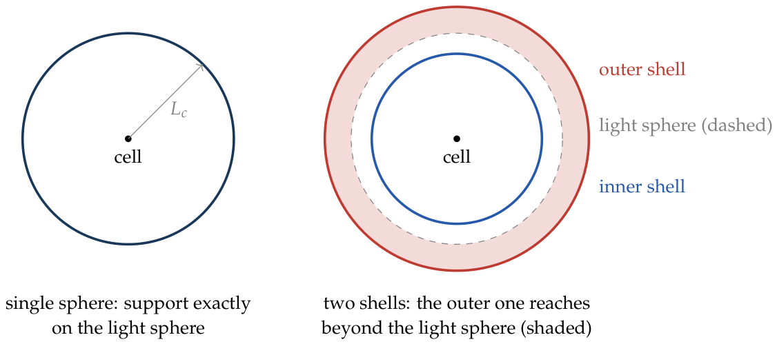
Disclaimer/Publisher’s Note: The statements, opinions and data contained in all publications are solely those of the individual author(s) and contributor(s) and not of MDPI and/or the editor(s). MDPI and/or the editor(s) disclaim responsibility for any injury to people or property resulting from any ideas, methods, instructions or products referred to in the content. |
© 2026 by the authors. Licensee MDPI, Basel, Switzerland. This article is an open access article distributed under the terms and conditions of the Creative Commons Attribution (CC BY) license (http://creativecommons.org/licenses/by/4.0/).
Copyright: This open access article is published under a Creative Commons CC BY 4.0 license, which permit the free download, distribution, and reuse, provided that the author and preprint are cited in any reuse.