

Submitted:
08 November 2026
Posted:
10 November 2026
You are already at the latest version
Abstract
In question answering (QA) for multi-constraint recommendation, the model must find every item that satisfies a request with several requirements. Still, training data that pair natural-language questions with complete answer sets are scarce. Such data can be synthesized by computing answers from an item catalog and using users’ ratings and reviews to select requests, yet the result may reveal whose evidence was used. We develop a QA data synthesis framework that protects these users using user-level differential privacy (DP), bounding each user’s total contribution and adding calibrated noise to the support statistics used to weight requests. Using one construction template, we build QA datasets for Movie, Beauty, and Recipe from pre-provided, rule-cleaned, and model-inferred attributes. In ablations without noise, an adversary who knows all other users’ data identifies, without false positives, every tested member whose evidence supports a request, up to 96% of members. Under DP with privacy budget ε=4, it flags at most 3.0% of members of these three datasets at a 1% false-positive rate, and an audit with repeated mechanism runs finds no evidence of privacy loss above ε. Models trained on private data retain at least 97% of the non-private ablation’s macro-averaged F1 on shared test questions.
Keywords:
synthetic question answering
; differential privacy
; multi-constraint recommendation
; membership inference
; privacy auditing
1. Introduction
Multi-constraint recommendation finds items that satisfy multiple user requirements simultaneously [1]. Training question-answering (QA) models for this task requires natural-language questions paired with their complete answer sets, and such data are scarce. pFoodReQ [2] and KERL [3] therefore build recipe QA data by synthesizing constrained questions and obtaining reference answers from a food knowledge graph. RecipeADQA [4] instead derives aspect-direction tags, each pairing a preference aspect with a direction, from real user queries and reviews. User histories can go further and indicate which combinations of constraints reflect real preferences. Ratings link users to items, and judgments extracted from reviews express support for or opposition to item properties [5]. Aggregating this evidence can shape the distribution of synthesized requests.
Such evidence is sensitive. Rating records can identify their owners even after anonymization [6], and synthetic data can retain information about their source records [7]. Because one user’s history may support many combinations of constraints, protecting a person requires bounding their total contribution. We therefore ask how to synthesize QA training data from this preference evidence while protecting the contributing users and retaining utility, the downstream performance of QA models trained on the synthetic data.
We propose a QA data synthesis framework with user-level differential privacy (DP), which bounds the change in the output distribution when one user’s complete evidence is added or removed [8]. Answers come from a fixed catalog, a structured collection of items and their attributes, and therefore do not depend on any user. Unlike general private synthesizers, which generate protected records such as table rows or preference data [9,10,11], the framework privatizes only support statistics, which count the users whose evidence supports each constraint combination and decide which combinations are sampled. It bounds each user’s total contribution to these statistics and adds calibrated noise to obtain sampling weights for requests.
We apply the framework to movies (Movie), beauty products (Beauty), and recipes (Recipe), with preference evidence drawn from MovieLens 32M ratings [12], Amazon Reviews 2023 ratings [13], and judgments extracted from Food.com reviews [14], respectively. All three express constraints as aspect-direction tags in the “aspect::direction” format of RecipeADQA, such as “genre::comedy”, “skin_type::dry”, or “health::low-sodium”. Movie uses pre-provided metadata, Beauty cleans product attributes with fixed rules, and Recipe uses preference tags inferred by language models. Each dataset pairs natural-language questions with structured constraints and complete answer sets.
The study makes three contributions:
- 1.
- Method framework. We introduce a QA data synthesis framework with a user-level privacy guarantee for the users whose ratings or review judgments supply preference evidence. The evidence adapter converts ratings or review judgments into binary support for constraint combinations that are fixed in advance. Requests with identical support for every possible user input share a single statistic, so a user’s bounded contribution is not split among them. Noisy sums of these bounded contributions then serve as sampling weights for QA pairs with complete catalog answers.
- 2.
- Multi-domain data construction. With one construction template and shared answer computation and dataset splits, we build Movie, Beauty, and Recipe in a common QA representation from pre-provided, rule-cleaned, and model-inferred aspect-direction tags with rating or review evidence.
- 3.
- Ablation-based privacy and utility evaluation. On outputs computed from the full user populations, we compare the full procedure of the framework with ablations that successively remove its noise and thresholding, its contribution bounding, and its user support. We evaluate membership-inference attacks that range from classifiers trained on additional releases with known membership to an informed adversary who knows every other user’s data, audit the implemented mechanism with repeated runs, and train QA models on each dataset to select, from a fixed candidate list, the items that satisfy each question. In the ablations without noise, the informed adversary identifies every member whose evidence supports at least one request; under DP with privacy budget , it flags at most 3.0% of the members of the three datasets at a 1% false-positive rate, even from the noisy support statistics before thresholding, which are not released. The audit finds no evidence of privacy loss above . Models trained on data from the full procedure retain at least 97.6% of the macro-averaged F1 of the non-private ablation, both on a test set shared by all models and on requests drawn in proportion to the support of users held out from synthesis, and without user support the request distribution lies 3.2 to 6.4 times farther from that support in total variation distance.
2. Related Work
2.1. Multi-Constraint Recommendation
Constraint-based recommendation represents user requirements through item properties and compatibility rules [1]. FoodKG [15] provides a food knowledge graph, and pFoodReQ [2] constructs a personalized QA benchmark whose reference recipes satisfy query requirements and dietary or health constraints. LC-QuAD [16] generates questions from query templates over DBpedia and pairs them with executable queries. QUEST [17] and RoMQA [18] pose questions with implicit set operations or many answers, and current retrieval and QA models struggle to recover their complete answer sets. Personalized recipe generation [19] and knowledge-enhanced recipe recommendation [3] use individual histories or external knowledge for personalization. RecipeADQA [4] derives an aspect-direction tag schema from real user queries and reviews and builds structured QA pairs for multi-constraint recipe recommendation. Across these QA datasets, however, constraint combinations come from templates, random sampling, or knowledge graphs and category structures rather than from user histories. We instead sample requests in proportion to the support each constraint combination receives in users’ ratings and review judgments, while answers remain complete sets computed from a fixed catalog. One construction template applies this design to movies, beauty products, and recipes.
2.2. Differentially Private Synthesis
Differential privacy (DP) bounds how much a mechanism’s output distribution can change between neighboring datasets, which are identical except for one record or for all records of one person [8]. The privacy budget sets this bound, and smaller values give stronger protection; a second parameter allows the bound to fail with a small probability, and gives pure DP. Applying DP to data synthesis requires specifying the privacy parameters, the unit of privacy, and the cumulative loss across all releases from the same data [20]. User-level protection bounds the combined contribution of all records from one person, trading bias from discarded contributions against noise [21].
McSherry and Mironov train recommenders on noisy aggregates of ratings, such as item averages and item–item covariances [22]. Private set union [23] releases elements contributed by enough users; because the candidate elements come from user data, the release threshold is part of its privacy guarantee and requires . The adaptive and iterative mechanism (AIM) [9] synthesizes private tabular data by adaptively selecting and measuring workload queries before generation, and DPPrefSyn [11] learns a private preference model and combines it with public prompts to generate preference data for language-model alignment. Without a DP guarantee, privacy-aware tabular generators can instead train an adversarial gradient-boosted tree generator under k-anonymization constraints [10]. None of these methods synthesizes questions paired with complete answer sets from a fixed catalog. Because our framework privatizes only the support statistics that weight requests, noise changes which requests are sampled but not their complete answers. The requests are fixed before any user data are read, and every statistic is subject to noise, so the release threshold adds no privacy cost, and the guarantee holds with .
2.3. Utility and Privacy Evaluation
The utility of private synthetic training data is commonly evaluated through the models trained on them. ContinuousBench [24], for example, tests whether private synthetic text transfers capabilities found only in the source corpus. On this benchmark, non-private synthesis transfers substantial corpus-specific knowledge, whereas current DP synthesis methods generally fail to do so even at , where protection is far weaker than at the budgets of 1 to 20 used in many deployments [20].
Membership-inference attacks test whether an observer of a release who knows a target’s data can tell whether those data were used to produce it [7]. Released aggregate statistics can reveal whether an individual contributed to them, as shown for allele frequencies [25] and aggregate location counts [26]. The power of such tests is bounded by the number of released statistics relative to the number of contributors [27], and tracing remains possible when the statistics are noisy [28]. Shadow models train attack classifiers on releases with known membership [29], and evaluation at low false-positive rates shows whether any individual is reliably identified [30]. Differences between the member and nonmember populations can, by themselves, make attacks appear successful [31]. Informed adversaries, who know every record except the target’s, remove this confound and match the neighboring datasets of DP [32]. Privacy audits use such adversaries, or repeated mechanism runs, to lower-bound the privacy loss of an implementation [33,34]. Attack outcomes therefore depend on the adversary’s knowledge and on the populations compared, and an unsuccessful attack does not establish that a release is private. Accordingly, we measure utility with QA models trained on each release, test the same releases with adversaries ranging from trained classifiers to an informed adversary, control for population differences, and audit the implemented mechanism with repeated runs.
3. Problem Formulation
3.1. Structured QA Pairs
Let be a fixed catalog of items and their attributes, such as the candidate recipe collection of RecipeADQA. Following RecipeADQA, a structured QA pair contains a natural-language question q, an executable constraint set C of atomic constraints on item attributes, and a verifiable answer set; a request is the set of requirements that C encodes and q expresses. To measure support in user histories, we partition C into a preference constraint core (hereafter, core), whose joint support is measured, and optional catalog-derived auxiliary constraints . The full constraint set and complete unordered answer set are
Here, means that item i satisfies constraint c, and the structured QA pair is . The partition is fixed for each request, with , although both parts may use the same tag vocabulary. Auxiliary constraints narrow the answer set, while support is measured on only.
For example, a review supporting “health::low-sodium” contributes to the core consisting of that tag, and adding an ingredient inclusion or exclusion constraint narrows the answers without changing this support statistic.
3.2. Support Units and the Synthesis Target
Let denote all preference evidence of source user u, the person whose rating history or extracted review judgments enter synthesis. A request bank is a fixed set of constraint combinations, grouped into support units that each share one support statistic. Unit has a fixed nonempty set of variants , each a complete constraint set, and all three domains group variants by their core. The support indicator equals one when the user’s input satisfies the support rule of and zero otherwise, and the support count before contribution bounding or noise is
The synthesis target is a population-level distribution over constraint combinations. Each unit carries a nonnegative weight, called its mass, such as its support count or a privately released weight. Request reconstruction (Section 4.3) converts these masses into . Private and non-private synthesis share this representation.
The fixed context comprises catalogs, schemas, request banks, semantic mappings or extractors, support rules, maps from units to variants, and language templates, all identical in neighboring datasets. A support indicator is user-local if it depends only on that user’s input and .
3.3. Privacy Scope and Outputs
The unit of privacy is one source user: two datasets are neighboring if one is obtained from the other by adding or removing all preference evidence of that user, with and every other user’s input unchanged. Movie and Beauty protect rating histories within fixed input populations. Beauty uses the provider’s 5-core population, in which every user and item has at least five interactions; this population is held fixed, so removing a user does not rerun the 5-core selection or change which other users and items are included. Recipe protects the judgments extracted from each user’s reviews, and the resources that extracted them are held fixed. Because identities in different sources may belong to one person, Section 4.4 also accounts for the privacy cost across domains. Table 1 summarizes, for each domain, what the guarantee protects, the resources it treats as fixed, and the steps it does not cover.
A release consists of constraint records, one for each variant of each retained unit, with their sampling weights. The C-only view exposes the constraint sets, and the C+weight view also exposes their weights; both derive from the same protected statistic. The C+weight view corresponds to releasing the synthesized data with their sampling frequencies, which carry the user-support signal, and the C-only view to releasing only the distinct constraint sets. Questions and complete answer sets are then generated from that statistic and fixed resources, without further access to protected inputs.
A membership adversary observes a release and part of a target user’s history, and predicts whether that user’s preference evidence was used in synthesis. Section 6 evaluates attacks on both views.
4. Method
Figure 1 gives an overview of the framework, which has three components. The evidence adapter (Section 4.1) encodes each source user’s rating history or saved review judgments as binary support over a request bank fixed before these inputs are read, and its support rule also determines which requests can share one statistic. The user-level private release (Section 4.2) bounds each user’s total contribution, adds calibrated noise, and thresholds the result to obtain sampling weights. QA pair sampling (Section 4.3) turns these weights into request probabilities, renders the sampled constraint sets as questions with fixed templates, and computes their complete answers from the catalog. Section 4.4 states the resulting privacy guarantee and its accounting.
4.1. Evidence Adapter
An evidence adapter supplies the support rule of Section 3.2, which computes from one user’s input and the fixed context. Because the domains provide two kinds of evidence, ratings and review judgments, the framework uses two kinds of adapters: rating adapters for Movie and Beauty and a review-judgment adapter for Recipe.
In the rating adapter, let be the items rated by user u, the rating of item i, and the mean over the complete supplied history, including items without usable catalog metadata. Define the positively associated catalog items as
For an executable constraint set T, rating support is
Here, is the indicator function. Support requires at least two distinct, positively associated items that satisfy every constraint in T, and each user contributes one binary indicator per unit, regardless of how many items match. The datasets Movie and Beauty apply Equation (4) to cores of one to three aspect-direction tags, , and an optional additional catalog attribute forms . Section 5 describes the catalog attributes and construction rules.
In the review-judgment adapter, let contain the supplied review contexts of user u, one per review. The judgments are saved model outputs that label each review sentence as supporting, opposing, or irrelevant to a candidate aspect-direction pair (Section 5); for context , and contain the pairs judged as “support” and “oppose”, respectively, and irrelevant judgments enter neither set. The user supports a core , a set of one to three aspect-direction pairs, if a single review context supports all of its pairs and opposes none of them:
Repeated sentence-direction judgments are deduplicated, and only explicit support enters . Multiple qualifying reviews from one user still yield one binary contribution per core, for the core of unit . The dataset Recipe applies this rule to the judgments that the RecipeADQA extraction pipeline saved for each user, and the aspect-direction tags map supported pairs to executable catalog constraints. Section 5 describes the review source, semantic resources, and catalog.
Under either support rule, units whose support is identical for every possible user input measure the same quantity, so counting them separately would split each user’s bounded contribution (Section 4.2.1) without adding information. Two units are support-equivalent if their support indicators agree for every admissible source-user input:
Support-equivalent units can share one exact support count. The equivalence depends only on the support rule and the fixed resources, so it is decided before any user input is read and costs no privacy budget.
Ratings attach to items, so rating support depends on a core only through the items it selects; review judgments attach to aspect-direction pairs, so review support depends on the pairs themselves. For ratings, Equation (4) depends on a core only through its complete answer set, so two rating cores with identical answers have identical support for every user and could share one statistic. However, the banks keep one unit per core in every domain, so that all three domains have the same unit structure and a quota of 1,024 cores. Review support in Recipe instead depends on the expressed directions: if the catalog returns the same recipes for “health::low-sodium” alone and together with “convenience::quick”, a review supporting only low sodium satisfies the first core but not the second under Equation (5), so Recipe cores with equal answers cannot share a statistic.
4.2. User-Level Private Release
The user-level private release turns the support indicators from the evidence adapter into the private weights used by request reconstruction (Section 4.3). All of its parameters and selection rules are fixed before any protected input is measured, because choosing them from the protected data would itself consume privacy budget.
4.2.1. Contribution Bounding and Quantization
Because one user may support many units, the release first bounds each user’s total contribution, so that adding or removing a user changes the aggregate by a limited amount, and scales the contributions to integers for the discrete noise added below. Encode user u’s support over the fixed bank as the binary vector , whose norm, the sum of its absolute entries, is the number of units that u supports. Let B bound each user’s total contribution and Q be a positive integer quantization scale. The bounded vector rescales when , the integer contribution quantizes its jth entry, and the bounded count sums these contributions over users:
A user supporting at most B units keeps and adds Q to each supported unit, whereas a user supporting units adds to each. Thus measures bounded support in user-equivalents, each equal to the contribution of one user who supports at most B units. When no user supports more than B units, . The bound applies once per user across the full bank, and users without matching evidence contribute zero but remain in the population.
The sensitivity of is its largest total absolute change between neighboring datasets. Because the coordinates are fixed and support indicators are user-local, adding or removing one user changes only by that user’s vector , whose norm satisfies . The sensitivity is therefore at most , and downward rounding removes less than user-equivalents from each user’s total.
4.2.2. Noise and Thresholding
One invocation of the randomized release mechanism, called a measurement, produces the noisy integer vector with
where is the noisy count of unit j and the noise terms are independent and follow the discrete Laplace, or two-sided geometric, distribution, with probability mass proportional to at each integer z [35]. Integer counts and discrete noise avoid the floating-point vulnerabilities of textbook Laplace samplers [36]. The scale divides the sensitivity by : adding or removing one user changes by at most in norm, so the probability of any noisy vector changes by at most a factor of , and a smaller adds more noise [37]. A user supporting units changes by at most and therefore incurs a privacy loss of at most in one release; only users supporting at least B units incur the full .
Every fixed coordinate receives noise, including those with zero support, so on the fixed bank this calibration gives pure DP with . An bound with Gaussian noise requires but reduces the per-unit weight of users above the bound in proportion to rather than , so users who support many units keep more weight [23].
Thresholding subtracts a fixed noise tolerance from each noisy count and keeps the positive results. For each bank, let be its total number of fixed support units across the three domains. For an accuracy level , is the two-sided discrete-Laplace accuracy tolerance at error probability , rounded up, and
By the union bound, the noise on all coordinates of a bank lies within with probability at least , and on this event . The parameter controls accuracy only; the DP relaxation parameter is . A unit is retained only when its noisy count exceeds , that is, when its noisy bounded support exceeds user-equivalents. The noise scale and the threshold grow in proportion to B: a smaller bound lowers the threshold but reduces the contributions of more users [21]. Each release uses one noise draw and a fixed threshold. If all are zero, the release is empty.
4.3. Sampling QA Pairs
QA pair sampling starts with request reconstruction, which maps support-unit masses to probabilities over the fixed variants. Let be the number of variants of unit j, and let be its mass, which in the private release is the weight of Equation (9). Units are sampled in proportion to their mass and variants uniformly within a unit, so unit j has probability and each variant has conditional probability :
The probability of a unit therefore does not depend on how many variants it has.
The marginal probability of a distinct full constraint set is . Because records retain their unit and variant identities, several records can share a single constraint set C, and sums their probabilities. Fixed templates render each sampled set as a question, and Equation (1) supplies its complete answer set, yielding a structured QA pair.
4.4. Privacy Guarantee and Accounting
Algorithm 1 combines the steps of Section 4.1, Section 4.2 and Section 4.3 into one mechanism, from evidence encoding to question rendering, and the guarantee below applies to this whole mechanism.
| Algorithm 1 QA data synthesis with user-level differential privacy |
|
Input: fixed context , support units with variant sets , complete supplied preference evidence , and Output: the requested release views and structured QA pairs, or an empty release
|
Proposition 1
(User-level privacy). For fixed context and user-local support indicators, Algorithm 1, denoted , provides ε-DP with for each source user’s supplied preference evidence: for any neighboring datasets and any measurable output event E,
Proof.
Section 4.2.1 bounds the sensitivity of by , so releasing with discrete Laplace noise of scale on every fixed coordinate is -DP [35]. Thresholding, empty-output selection, reconstruction, view conversion, template rendering, and constraint evaluation over the fixed catalog depend only on and fixed context, and the post-processing property [8] preserves the guarantee for their joint output. □
Each release is one measurement. Its C-only and C+weight views, and any model trained on its QA data together with fixed resources, are post-processing of and keep the guarantee of Proposition 1, whereas every further measurement of protected inputs adds privacy cost. Sequential composition [8] adds the privacy costs of measurements that involve the same person, including measurements in different domains (Section 3.3).
5. Dataset Construction
We build Movie, Beauty, and Recipe with the framework of Section 4 and one construction template, so the three datasets share the private release, request reconstruction, answer computation over the catalog, and splitting rules. Their construction differs only in the provenance of the aspect-direction tags, the evidence for core support, and the auxiliary constraints, which Table 2 compares. Movie and Beauty take their tags from pre-provided metadata, which Beauty cleans with fixed rules, whereas Recipe infers them from reviews with large language models (LLMs) and a small language model (SLM).
5.1. Data Sources
Movie combines MovieLens 32M ratings [12,38] with pre-provided metadata in five aspects: genre and release decade from MovieLens, with 19 and 16 directions, and runtime, original language, and production country from a snapshot of The Movie Database (TMDB) [39]. The snapshot covers the 86,244 of 87,585 catalog movies whose MovieLens link resolves to a TMDB entry. Runtime has three directions, short, medium, and long (under 90, 90–119, and at least 120 minutes), and language and country keep their ten most frequent values, for 58 directions in total. The metadata define the constraints, and ratings determine support for their conjunctions.
Beauty uses the official Amazon Reviews 2023 Beauty_and_Personal_Care 5-core ratings [13,40] and six aspects, with 3,776 scent, 883 material, 645 item-form, 638 category, 289 hair-type, and 33 skin-type directions after the cleaning below. Fixed rules normalize values, split multi-valued fields when every part is interpretable, and merge aliases within a field, keeping all applicable values and excluding unresolved ones from evidence. Brand is excluded because its 51,950 values formed 89% of the eligible attribute constraints and would let brand-specific combinations dominate catalog-derived requests. The values hair_type::all and skin_type::all, which state that a product suits every hair or skin type, serve only as auxiliary constraints, since they describe broad applicability rather than a preference. The catalog contains 1,028,914 products, and 6,262 of the 6,264 directions can enter cores.
Recipe uses Food.com review judgments [14] and the semantic resources of RecipeADQA [4]. RecipeADQA identified nine user preference aspects from recipe-related queries in the ORCAS query-click dataset [41], took their fine-grained directions from Food.com reviews, and retained 393 aspect-direction pairs supported by reviews. It built this vocabulary and 100,000 silver labels for sentence-direction records with GPT-5.5 [42], Qwen3.5-9B [43], and DeepSeek-v4-flash [44], and fine-tuned the SLM, a DeBERTa-v3-base natural language inference (NLI) classifier [45], on these labels. The SLM classifies each review sentence as support, oppose, or irrelevant for each candidate aspect-direction pair, with 0.811 test accuracy against the silver labels. The recipe catalog is RecipeADKG, the enhanced recipe knowledge graph that RecipeADQA built from FoodKG and its underlying Recipe1M+ resources [15,46]; it maps 8,701 normalized FoodKG tags to 379 aspect-direction pairs over 706,350 recipes. Review judgments on the 335 pairs in both sets can be evaluated as executable tag constraints; by aspect, these pairs comprise 77 region, 61 tool, 52 occasion, 44 taste, 39 health, 27 method, 14 audience, 13 convenience, and 8 quantity directions. Our review-judgment adapter groups the saved judgments by review and by user, identified by the review’s author ID, with Equation (5).
5.2. Request Banks and User Roles
The main bank of each domain follows one construction template; Section 6.1.1 adds a random bank for comparison. A core combines one to three aspect-direction tags that are eligible as evidence and co-occur in at least one catalog item, and in Movie and Beauty it must match at least two items, the minimum for rating support. Each main bank keeps 1,024 cores, divided equally among the three core lengths and ranked within a length by the number of catalog items they match, with seeded tie-breaking. A length with fewer eligible cores, such as the 58 single-tag cores of Movie, passes its unused quota to the others.
For each core, the options are the core alone and the core extended by one additional catalog attribute. Construction ranks the options by the distance of their answer counts from 20 and keeps as the unit’s variants those among the first four that have L to 25 complete answers, with in Movie and Beauty and in Recipe. The cap of 25 follows RecipeADQA, which sets it from the average answer count of 25 at its maximum of ten constraints [4]. In Recipe, options with more than 25 answers are first narrowed toward 20 answers by adding ingredient inclusion or exclusion constraints, as in RecipeADQA [4], within the ten-constraint limit. Sixteen of the 4,060 main-bank variants carry such constraints. Cores without an accepted option are dropped and not replaced, leaving 1,021, 1,021, and 1,024 units in the main banks (Table 3). Complete answer sets come from evaluating the final constraints against the catalog.
Table 3 reports the source populations and dataset sizes. A fixed pseudorandom assignment divides the eligible users of each source into five disjoint roles in the proportions 20:50:10:10:10: auxiliary users, construction users, attack-reference users, nonmembers, and reference users. In Movie and Beauty, auxiliary users are the only users whose ratings may inform the design of the fixed resources, so that no construction user influences the fixed context; in every domain, auxiliary users enter no reported release or experiment. All 600,975 construction users enter construction, including those with zero support, and member targets are drawn from them; attack-reference users join the additional synthesis runs that train and calibrate the membership-inference attacks, nonmembers join no synthesis run and are scored by these attacks, and 5,000 reference users per domain, taken from their role in a fixed pseudorandom order, also join no synthesis run and provide held-out user support for evaluating the synthesized requests and the trained models.
5.3. Utility Test Set
Utility is measured by how well QA models trained on each dataset select, from a fixed candidate pool, the items that satisfy each question, so each domain fixes a test set of 400 questions that every such model answers (Table 3). Test requests are drawn from the main bank independently of user support: its variants are grouped by constraint count, ordered pseudorandomly within each group with a fixed seed, and taken from the groups in rotation until 400 distinct constraint sets are chosen. Each domain also has a validation set of 40 requests for model selection, whose answer sets are distinct and disjoint from those of the test set; it is drawn from the main bank in a fixed pseudorandom order, and the reported models, trained with fixed settings and evaluated with their final weights, do not use it. Training, validation, and test questions use distinct fixed template families, while catalog items may recur across these splits. Table 4 shows one test request per domain.
A fixed template renders each test request as a question, whose candidate pool of 30 items all models of a domain see in the same order. As in RecipeADQA [4], the pool contains all correct answers and distractors that violate at least one constraint, with priority to items that violate few constraints.
Training holdout keeps validation and test requests out of training: it removes from every training set each request whose full constraint set matches that of a validation or test request, together with requests that share the complete answers of a validation request or of half of the test requests (Appendix D).
6. Experiments
On the datasets of Section 5, we evaluate the full procedure of Algorithm 1 against ablations of its components and against a random request bank (Section 6.1.1), with three research questions on utility, fidelity to user support, and membership inference, answered in Section 6.2, Section 6.3 and Section 6.4:
- RQ1.
- How do the components of the full procedure and the construction of the request bank affect candidate-selection utility?
- RQ2.
- How closely do the request distributions of the full procedure and its ablations reflect reference-user support, and how well do the trained models answer requests drawn in proportion to that support?
- RQ3.
- How detectable is membership in the releases of the full procedure and of its ablations without noise to trained, realistic, and informed adversaries, and does an audit of the implemented mechanism find privacy loss above the stated bound?
6.1. Experimental Setup
This section gives the settings shared by all research questions; the protocols specific to fidelity and membership inference precede their results in Section 6.3 and Section 6.4.
6.1.1. Synthesis Settings
Each domain has two request banks: the main bank of Section 5 and, for comparing bank construction (RQ1), a random bank. The random bank keeps the number of main-bank units of each core length, but it orders eligible cores pseudorandomly with a fixed seed instead of by match count and builds variants by random sampling adapted from the knowledge graph question-answering (KGQA) generation of KERL [3], in the form reconstructed for RecipeADQA [4].
Each variant is built from a sampled catalog item that satisfies the core: in Movie and Beauty, it adds a random subset of the item’s other attributes, and in Recipe, it adds inclusions of the item’s ingredients and exclusions of ingredients that the item lacks but other recipes satisfying the core contain. Each core keeps up to four distinct variants within the domain’s answer-size bounds and the ten-constraint limit, and the cores with accepted variants form the random bank (Table 3).
Both banks are fixed before protected support is measured and share source populations, support rules, constraint evaluation rules, and privacy parameters. They differ only in their request spaces and hence in the user evidence they match.
Each bank has four procedures, which differ only in the unit masses passed to request reconstruction (Section 4.3): the full procedure and three ablations that remove its components cumulatively:
- DP The full procedure of Algorithm 1: the thresholded noisy mass .
- Bounded-non-private (Bounded) Without noise and thresholding: the bounded, quantized count of Equation (7).
- Non-private (NP) Also without contribution bounding: the unbounded support count .
- Public-only (Public) Also without user support: equal mass on every fixed unit, from fixed resources only (Table 1).
Each domain thus has eight training sources, one per bank and procedure; we name a source by its bank and procedure, as in main DP or random NP, and tables omit the prefix “main”. Each ablation is compared with the full procedure: DP minus Bounded measures the effect of noise and thresholding, DP minus NP that of the whole private release, and DP minus Public that of protected-user support, while comparing Bounded with NP isolates contribution bounding. Bounded and NP show what the private release costs in utility and provides against membership inference, and Public shows what user support adds to the fidelity of the request distribution. Main DP minus random DP compares bank construction at a common privacy budget.
All releases use , , , and . The bound B trades bounding against noise (Section 4.2.2), and keeps the rounding loss below 0.001 user-equivalents per user. The noise scale is then 5 user-equivalents, so a user supporting units incurs a privacy loss of at most per release. With for the main bank and 2,888 for the random bank (Table 3), the thresholds are 55.1 and 54.8 user-equivalents. Because the discrete-Laplace tail decays exponentially, grows only with : doubling a bank would raise it by , about 3.5 user-equivalents. The mechanism is implemented with OpenDP 0.15.1 [47].
The releases from the main and random banks of a domain measure the same users, so by sequential composition (Section 4.4) a user in both incurs a privacy cost of at most per domain and at most 24 across the three domains. The ablations and the fidelity measures of Section 6.3 are computed outside Algorithm 1, without a privacy guarantee, and only their aggregate results are reported.
6.1.2. QA Training and Evaluation
We train one QA model on each training source of Section 6.1.1 and evaluate it, together with a Base model that receives no fine-tuning, on the test set of Section 5.3. A model receives the question and the attributes of each candidate, labeled by a short code that is unique within the question, and answers with the codes of the selected items.
As in RecipeADQA [4], all adapted models fine-tune Qwen3-1.7B [48], which also serves as the Base model, with low-rank adaptation (LoRA) [49] under identical settings (Appendix D). Each model is trained once on the reported QA data of its training source, with the same input-token budget of 2,097,152 tokens: examples are drawn with replacement from the source’s request distribution after training holdout until their prompt and answer tokens reach this budget. Because the budget fixes training length, supervised-token counts, optimizer steps, and the coverage of sampled records vary across training sources. Each question is then decoded once greedily, with the final LoRA weights for adapted models; the eight adapted models and the Base model of each domain give 27 evaluations of 400 questions, or 10,800 predictions.
We score each prediction against the complete answer set of its question. A valid response is a JavaScript Object Notation (JSON) object holding a single list of unique codes. Invalid responses, including those with duplicate codes, count as empty predictions, and codes absent from the candidate list count as false positives. For question i, let be the codes of all qualifying candidates and the predicted codes. Precision is the fraction of predicted codes in , and recall is the fraction of recovered. The primary metric is the mean of per-question F1 scores:
Because every is nonempty, an empty prediction has F1 of zero. The share of NP macro F1 that DP retains is their ratio within a bank and domain. Exact match (EM) requires a valid response whose predicted set equals , and format success is the rate of valid responses; all three metrics average over the full test set.
Intervals for the QA metrics use 2,000 paired cluster bootstrap replicates per domain [50]. Each replicate resamples groups of questions with identical complete answers and shares its draws across models, and the resulting pointwise intervals are not adjusted for multiplicity. They condition on the fitted models, candidate sets, and released datasets and do not cover variation between training runs, because each model is trained once.
6.2. Utility Performance
6.2.1. Ablations
On the test set, models trained on data from the full procedure retain 97.6% to 100.0% of the macro F1 of the NP ablation (Table 5), and the DP minus NP difference excludes zero only in Beauty, at points (; Table 6). This cost lies in precision: the DP model recovers the correct answers as completely as the NP model, with mean recall of 99.1% against 98.9%, but also selects more distractors, with mean precision of 89.9% against 93.8%. In EM, the DP minus NP difference also excludes zero only in Beauty, at points (), a larger gap than in F1, because a single selected distractor fails a question.
Noise and thresholding remove every unit whose noisy count falls below , whereas the test set, drawn independently of user support, still asks about these units. Bounded, which omits the two steps, exceeds DP by 4.83 points in Beauty, where DP keeps fewer than half of the request variants (Table 3), and by 0.24 points in Movie, where it keeps most of them. In Recipe, DP keeps only about a third of the variants, yet no ablation, not even Public, which covers every unit, differs from it in F1, so F1 there depends little on which units the training data cover.
The Public ablation, which removes user support, spreads its mass evenly over the main bank and trains on 1.1 to 3.0 times as many records as DP; with intervals excluding zero, it is 5.97 points higher than DP in Beauty and 0.79 points lower in Movie. Because the test set ignores user support, it quantifies the utility cost of the private release relative to NP but cannot show what user support contributes; Section 6.3 examines how closely the private weights follow that support and how the models answer requests drawn by it.
F1 rewards partial answers: test questions have about 17 correct candidates out of 30, so the all-candidate heuristic, which selects every candidate, reaches F1 of 67.74% to 72.32% with zero EM. Differences between adapted models reflect selection rather than output format, because every adapted model produces valid responses for at least 99.50% of questions, whereas Base does so for at most 5.75% and scores near zero; Table A1 reports all 27 evaluations.
6.2.2. Bank Construction
The main bank yields more useful training data at the same privacy budget: at per release, main DP exceeds random DP in F1 in all three domains, by 0.22 to 19.63 points, and in EM in Beauty and Recipe, with intervals excluding zero (Table 6). Because the test set is drawn from the main bank, these gaps also reflect how well the training requests of each bank cover the test requests, and the two large gaps, in Beauty and Recipe, have different sources.
In Beauty, the gap comes from user support. Main-bank cores, ranked by catalog match count, match more items and hence more users’ ratings: 25.56% of reference users support at least one main-bank unit, against 2.06% for the random bank (Table A2). Because a unit needs about 55 user-equivalents of support to pass the threshold, main DP retains 1,698 request variants, whereas random DP retains 36 (Table 3). In Recipe, the banks reach similar user coverage, and the gap comes from the request space: random-bank variants combine a core with several ingredient constraints and have 1.87 complete answers on average, against 18.74 in the main bank, so models trained on them select too few items. Even random Public, which covers every random-bank unit, has a mean recall of only 37.6% at a mean precision of 96.1%.
6.3. User Support Fidelity
6.3.1. Distributional Fidelity
To answer RQ2, we encode the 5,000 reference users of each domain with the same support and reconstruction rules, after the banks, training sources, and model settings are fixed, and compare each source distribution, before training holdout, with their support through three fidelity measures.
User coverage is the fraction of reference users supporting at least one retained unit. Mass coverage is the fraction of reference support mass captured by retained units under the reconstruction rule. The reference target is the request distribution that reconstruction assigns to reference-user support, and the total variation (TV) distance between a request distribution p and is
A lower TV means that the request distribution follows the preferences of the held-out reference users more closely. The raw reference target uses unbounded support, and the bounded reference target applies the mechanism’s contribution bounding and quantization; each comparison stays within one bank, because the two banks define different request spaces.
DP keeps the request distribution close to reference-user support, because the units that its threshold removes have few supporters and together hold little support mass. Although thresholding removes up to two-thirds of the request variants (Table 3), DP retains over 96% of reference support mass and nearly the user coverage of NP in every domain (Table 7). With the same bank, user support makes the distribution follow users: Public, which spreads its mass evenly over the same bank, lies at TV distances of 0.41 to 0.73 from the raw reference targets, 3.2 to 6.4 times those of DP.
DP’s distance of 0.11 to 0.15 from the raw reference targets has three sources. Noise and thresholding add only 0.011 to 0.026 to the distance of Bounded. Comparing against the raw and bounded reference targets isolates contribution bounding, which matters mainly in Movie, where 95.0% of the member targets support at least 20 main-bank units, against at most 3.5% in Beauty and Recipe: there, DP and Bounded lie within 0.016 of the bounded target but 0.12 to 0.13 from the raw target, so bounding accounts for most of their distance from raw support (Table A2). NP, which applies the same reconstruction rule to the exact support of the construction users, differs from the raw target only through sampling variation between construction and reference users; this variation is largest in Beauty, where the fewest reference users support any unit, and there NP lies nearly as far from the raw target as DP.
6.3.2. Preference-Weighted Test
The DP, Bounded, and NP training sources weight requests by the support of construction users, whereas the test set ignores support. To evaluate the trained models on the requests that users support, we build a preference-weighted test set, whose requests are drawn in proportion to the support of the held-out reference users. In each domain, 400 draws select main-bank units with probability proportional to their number of reference supporters, with a fixed seed per domain. Each draw receives a request of its unit that is absent from both banks and from the test and validation sets, and a draw fails when its unit has no such request (Appendix D). Questions use the candidates and template of the test set and are weighted by their number of draws. The four main-bank models of each domain, the same fitted models as on the test set, answer these questions without retraining. Intervals for the preference-weighted test set use 2,000 paired bootstrap replicates of the draws.
The preference-weighted test set represents reference-user support with requests that no training source contains. Of the 400 draws per domain, 348 to 395 succeed, and units with failed draws hold at most 8.0% of the draw probability; nearly all successful draws have answer sets absent from every training source. Their units lie in the DP training sources for at least 96.3% of draws, because the units that reference users support most also have enough support among construction users to pass the threshold.
On these requests, DP matches NP: their F1 differs by at most 0.51 points in every domain, with intervals that include zero, and DP lies at most 3.44 points below Bounded (Table 8). The Beauty cost on the test set thus falls on requests that users rarely support, which the threshold removes and the preference-weighted test set seldom draws. For the same reason, the advantage of Public over DP in Beauty shrinks from 5.97 to 1.54 points, with an interval that still excludes zero, while DP remains significantly above Public in Movie and close to it in Recipe.
6.4. Membership Inference
The membership experiments of RQ3 apply the adversary of Section 3.3 to the releases of each bank and domain. In each domain, the targets are 5,000 member targets, who participate in synthesis, and 5,000 test nonmembers; 5,000 further calibration nonmembers serve only to set attack thresholds. Attackers observe the complete released constraint set, and in the C+weight view its sampling weights, before training holdout or sampling. They know a partial history of each target: 20 of its rated items in Movie and Beauty, or five of its review contexts with their saved judgments in Recipe, selected pseudorandomly with a fixed seed (Appendix D). Targets with short histories or no matching evidence remain in the evaluation.
All releases in these experiments share a background of every construction user except the 5,000 member targets. A shadow release, an additional synthesis run with known participation used to train or calibrate an attack [7,29], adds 5,000 attack-reference users to , whereas the target release, from which the reported datasets come, adds the member targets, so all releases have the same population size. Shadow-training and shadow-calibration releases draw from separate pools of 10,000 attack-reference users, and paired shadow releases add complementary halves of a pool, so 20,000 attack-reference users take part. Each bank–domain pair has 32 shadow-training releases, 16 shadow-calibration releases, and one target release.
True positives (TP) are members the attack identifies, and false positives (FP) are nonmembers it flags; the true-positive rate (TPR) and false-positive rate (FPR) divide these counts by the 5,000 member targets and the 5,000 test nonmembers. Each attack’s threshold is calibrated on the calibration nonmembers to a 1% FPR target, and a target is flagged when its score strictly exceeds the threshold. We report TP, FP, TPR, FPR, and the area under the receiver operating characteristic curve (AUC), with score orientation fixed in advance. Attack intervals use 2,000 paired bootstrap replicates that resample members and nonmembers separately and condition on the fitted attacks, thresholds, shared backgrounds, and the noise draw of each target release.
Each shadow release is an additional measurement of protected inputs, because it contains the background ; the attacks and controls below reuse the completed releases and fitted classifiers, and the audit runs on synthetic inputs, so none of them adds a measurement. The DP outputs reported in this paper thus rest on 294 measurements, 49 for each of the six bank–domain pairs, with a conservative sequential sum of for a person involved in all of them, whereas each released dataset carries its per-release guarantee.
6.4.1. Trained Attacks
Two trained attacks are L2-regularized logistic regressions fitted on the shadow-training releases: an aggregate classifier summarizes the target’s observed support and its agreement with the release, and a per-unit classifier adds indicators of supported and released units and, in the C+weight view, released weights. An untrained matching score serves as a third attack: the summed released weight of the target’s matched units in the C+weight view, or their released fraction in the C-only view. All three attacks run on both views, and the C+weight per-unit classifier on all targets is the primary attack. For the primary attack, approximate simultaneous intervals [51] cover, per domain, a fixed family of seven comparisons (Appendix C) and ten metrics: AUC, average precision, equal error rate, standardized partial AUC below 1% FPR, and TPR, FPR, and attack advantage (TPR minus FPR) at the 1% target and an additional 5% calibration target. Their familywise level is 0.05/3 per domain, which splits 0.05 across the three domains.
Because the trained classifiers learn from few shadow releases, they can respond to differences between the member and nonmember populations rather than to the release. Two negative controls assess this effect. In the first, the trained classifiers, frozen after fitting, score the targets against the 16 shadow-calibration releases, which contain no target and thus serve as placebo releases, with thresholds recalibrated on each release. Detections on placebo releases can come only from population differences, so an actual release whose AUC or TPR exceeds the placebo range reveals membership through the release itself. In the second, a blind baseline [31], a logistic regression on the same partial-history features, is evaluated by five-fold cross-validation and measures how well members and nonmembers can be separated without any release. In addition, detections are split by whether the target’s partial history matches at least one unit, because only such targets give an attack release-based evidence.
The trained attacks stay close to chance on every release, including the Bounded and NP ablations, which add no noise: the primary attack has AUC from 0.487 to 0.533 on the main-bank releases (Table 9), and the trained classifiers have AUC from 0.490 to 0.509 on the C-only views of both banks. A target changes each supported count by at most one user-equivalent among 100,394 to 364,798 construction users, which is small against the variation that the other users contribute, so to an adversary who does not know their contributions, a release reveals little about any single target [27,28]. Every detection at the calibrated threshold comes from a target whose partial history matches at least one unit.
With so little leakage to remove, DP’s advantage over the ablations reaches significance only against Bounded, whose releases give the primary attack the most detections. In Recipe, the attack has lower AUC and TPR against DP than against Bounded, by 0.029 in AUC and 1.02 percentage points in TPR, with approximate simultaneous intervals and , although the interval for attack advantage includes zero; in Beauty, only its TPR at the 5% calibration target is lower, by 1.46 points. Against NP, every interval in these two domains includes zero, and in Movie no comparison in the multi-metric family excludes zero (Appendix C).
The negative controls show that the small excess of the Bounded and NP releases comes from the releases themselves rather than from differences between the member and nonmember populations. Without any release, the two populations can hardly be separated: the blind baseline reaches AUC of at most 0.509. On the placebo releases, which contain no target, the AUCs of the primary attack stay below the actual Bounded and NP AUCs in all three domains, and its TPRs below theirs in Beauty and Recipe, whereas every actual DP TPR lies within its placebo range (Table A3); noise thus removes the detections that the non-private releases add. Because these attacks gain so little even without noise, however, they cannot show how much protection the noise provides; the likelihood-ratio attacks of Section 6.4.2 test the support statistics directly, up to an adversary who knows every other user’s contribution.
6.4.2. Likelihood-Ratio Attacks
Two likelihood-ratio attacks test the support statistics directly, as in membership tests on aggregate genomic data [25,27]: a realistic adversary, who has reference statistics as side information, and an informed adversary, who knows every other user’s contribution. For DP and Bounded, the realistic adversary receives more than the release: the unthresholded noisy vector and the bounded counts , which are not released but from which either view can be computed. For NP, it recovers the support counts from the C+weight view, which determines them up to a common factor. From the support of the 20,000 attack-reference users, it predicts each unit’s support count among the construction users with a negative-binomial distribution (Appendix D). A target’s score then asks whether the statistics it observes are better explained with or without the target among the supporters: it sums, over the units matched by its partial history, the log-likelihood ratio between one additional supporter and none. Under DP, the predicted count is convolved with Laplace noise of scale five user-equivalents, and the C-only score uses the probabilities that the noisy counts exceed .
The informed adversary knows the contributions of every other construction user and the target’s complete contribution , so its two hypotheses, with and without the target, are the neighboring datasets of Proposition 1[32]. For DP, it computes the log-likelihood ratio between these hypotheses on and on each released view (Appendix D); for Bounded and NP, it compares the released views with those computed with and without the target. Target t changes its coordinates by , so its privacy loss is at most , where is its number of supported units (Section 4.2.2). For targets with , the expected TPR at any threshold is therefore at most times the expected FPR, the limit against which the detection rates of this adversary are compared.
Table 10 reports the likelihood-ratio attacks on the main-bank target releases. Exact support counts do not help the realistic adversary: it recovers them from the C+weight view of NP, yet its AUC ranges only from 0.498 to 0.518 across all releases of both banks, with similar TP and FP counts at the calibrated threshold, and the unthresholded DP vector does not change this result. Its prediction of each count from the 20,000 attack-reference users remains uncertain by more than the single supporter that a target adds, so, as for the trained attacks, the unknown contributions of the other users hide the target.
The informed adversary, who knows these contributions, faces no such uncertainty. In the C+weight views of the Bounded and NP ablations, which release support statistics without noise, it identifies, without false positives, every member who supports at least one unit, up to 4,788 of the 5,000 members in Movie, so contribution bounding alone gives no membership protection; the C-only views expose only members who are the sole supporters of some unit, at most one per domain, because removing any other member leaves the set of released units unchanged. Noise prevents this exposure. Even from the unthresholded noisy vectors, which are not released, the adversary flags at most 3.0% of the 5,000 members, 151 in Movie, and from the released views at most 1.6%, 79 in the C+weight view of Recipe; both rates lie far below the TPR of about 55% that permits at a 1% FPR. The random bank shows the same contrast, with at most 476 detections in random Movie (Table A4).
Detection under DP stays far below this limit because bounds the log-likelihood ratio of every outcome, whereas detection depends on its typical value. For the unthresholded attack, the expected log-likelihood ratio, the Kullback–Leibler divergence between the distributions of with and without a member’s contribution, grows as about for a member supporting units and falls to about beyond the bound, where bounding spreads the same total contribution over more units. Detection follows this pattern: in Beauty and Recipe, it rises up to members supporting 10 to 19 units, of whom the adversary flags 27.3% in main Beauty, against 11.5% of comparable nonmembers, and in every DP release with members in both groups, those supporting at least 20 units are flagged less often, for example 7.8% against 36.7% in random Movie. In main Movie, whose members support 237 units on average, 141 of the 151 flagged members belong to the 4,748 members supporting at least 20 units, a rate of 3.0%, against 1.0% for comparable nonmembers.
6.4.3. Mechanism Audit
Because all targets of a release share a single noise draw, the detection rates of the likelihood-ratio attacks reflect the actual releases; to estimate per-target privacy loss, we audit the implemented mechanism using synthetic canaries and repeated, independent runs of the mechanism [33,34]. A canary is a synthetic user that each trial either includes in the input or leaves out. It supports k units with contributions from Equation (7), so its privacy loss is (Section 4.2.2): the values , 5, 20, and 40 lie below, at, and above the bound and give losses of 0.2, 1, 4, and 4. Each supported unit receives mass from other users, so the expected counts with and without the canary lie symmetrically around the release threshold. Half of the trials select the score orientation and threshold of the likelihood-ratio statistics on and on the C-only view; the other half give from one-sided 97.5% Clopper–Pearson limits, a 95% lower confidence bound [52]. Two mechanisms that violate the stated serve as controls: a noise-free mechanism, whose outputs with and without the canary never coincide, so its privacy loss is infinite, and one with half the noise scale, whose true is 8.
In Table 11, the audit finds no evidence of privacy loss above the stated , and its controls show that it detects mechanisms that exceed it. Every 95% lower bound stays below the loss of its canary. For a one-unit canary, the bound nearly reaches the loss, 0.188 against 0.2, because the likelihood ratio of a single unit reaches its maximum on about half of the outcomes; a canary spread over 20 units reaches its loss of 4 only on rare outcomes, so its bounds stay near 2.3 even with 1,000,000 trials, and the 40-unit canary, with half the contribution per unit and fewer trials, gives lower bounds still. Without noise, the bound reaches 10.208, the largest value that the 100,000 evaluation trials per hypothesis allow, and at half the noise scale, where the true loss is 8, the bounds of 4.199 to 4.435 exceed the stated while staying, as for the 20-unit canary, well below the true loss.
7. Discussion
Privacy costs little utility because noise changes only which requests are sampled and how often: unlike private text synthesis, whose generated text must carry the protected knowledge [24], every retained request keeps its complete answer set. The test set measures this utility at the selection step of a retrieval-augmented recommender: its candidate pool acts as a retriever that returns every correct item among near-miss distractors, so differences between models reflect their training data rather than retrieval.
Without noise, a release protects its users only from adversaries who do not know the other users’ data (Section 6.4). Noise removes this dependence on the adversary’s knowledge, and contribution bounding lets noise of five user-equivalents suffice but gives no membership protection by itself. The guarantee is weakest for users who reach the bound: every user supporting at least 20 units incurs the worst-case loss , and protecting these users more strongly requires a smaller , which raises the threshold and removes more requests.
The same private aggregation serves three constraint vocabularies and two kinds of evidence, but the domains differ in how many units their users support: most Movie users exceed the bound, so bounding moves the Movie distribution away from raw support, whereas few users in Beauty and Recipe reach it (Section 6.3). All three domains share ; a domain-specific bound would set the trade-off between bounding bias and noise separately in each domain [21].
8. Conclusions
Our framework synthesizes multi-constraint QA data from ratings and review-derived judgments while protecting the contributing users with user-level differential privacy. Users affect only the sampling weights, which are noisy sums of their bounded contributions to the support of fixed requests, whereas complete answers come from a fixed catalog. One construction template produces Movie, Beauty, and Recipe from pre-provided, rule-cleaned, and model-inferred aspect-direction tags.
In ablations without noise, an adversary who knows every other user’s data identifies every member who supports at least one unit; at per release, it flags at most 3.0% of members in the private releases from the main bank at a 1% false-positive rate, even when given their unthresholded noisy vectors, which are not released. Attacks without such knowledge remain near chance on every release, including those without noise, and an audit with repeated mechanism runs finds no evidence of privacy loss above the stated budget.
Models trained on data from the full procedure retain 97.6% to 100.0% of the macro F1 of the NP ablation on the test set and stay within 0.51 points of it on requests drawn in proportion to user support. At the same privacy budget, models trained on main-bank data achieve higher F1 than those trained on random-bank data in all three domains. The private request distributions retain over 96% of reference support mass, whereas the request distribution of the Public ablation, which ignores user support, lies 3.2 to 6.4 times farther from reference-user support in total variation distance.
Author Contributions
Conceptualization, S.J. and Y.M.; methodology, S.J.; software, S.J. and H.L.; validation, S.J.; formal analysis, S.J.; investigation, S.J. and H.L.; data curation, S.J. and H.L.; writing—original draft, S.J.; writing—review, S.K., K.M.R.A., and Y.M.; supervision, S.K., K.M.R.A., and Y.M.; funding acquisition, S.J., K.M.R.A., and Y.M.; project administration, Y.M. All authors have read and agreed to the published version of the manuscript.
Funding
This work was supported by JSPS KAKENHI Grant Number JP25K15130 and JST SPRING Grant Number JPMJSP2132.
Institutional Review Board Statement
Not applicable.
Informed Consent Statement
Not applicable.
Data Availability Statement
The implementation, the three released datasets with their request banks and data splits, and the aggregate results of this study are available at https://github.com/MorimoLab/PrivacyQA. The Beauty data are released in full. For Movie and Recipe, item attributes derived from TMDB and Recipe1M+, whose terms do not permit redistribution, are withheld, along with the candidate lists and answer sets that depend on them; the repository describes how to rebuild them from the original sources. The source data are available from their providers: MovieLens 32M [38], Amazon Reviews 2023 [40], Food.com reviews [14], the TMDB API [39], and the RecipeADQA resources at https://github.com/MorimoLab/RecipeADQA, with Recipe1M+ and FoodKG under their own terms [15,46].
Acknowledgments
OpenAI Codex and Anthropic Claude assisted with manuscript drafting, restructuring, and LaTeX preparation. The authors have reviewed and edited the output and take full responsibility for the content of this publication.
Conflicts of Interest
The authors declare no conflicts of interest.
Abbreviations
The following abbreviations are used in this manuscript:
| AIM | Adaptive and iterative mechanism |
| AUC | Area under the receiver operating characteristic curve |
| DP | Differential privacy |
| EM | Exact match |
| FP | False positive |
| FPR | False-positive rate |
| GPU | Graphics processing unit |
| JSON | JavaScript Object Notation |
| KGQA | Knowledge graph question answering |
| LLM | Large language model |
| LoRA | Low-rank adaptation |
| NLI | Natural language inference |
| NP | Non-private |
| QA | Question answering |
| RQ | Research question |
| SLM | Small language model |
| TMDB | The Movie Database |
| TP | True positive |
| TPR | True-positive rate |
| TV | Total variation |
Appendix A. Complete Test-Set Results
Table A1 reports all 27 model evaluations, with intervals from the paired cluster bootstrap of Section 6.1.2.

Table A1.
Test-set results of all 27 model evaluations. Train is the number of training records after training holdout; macro F1, EM, and format success are percentages, with 95% paired bootstrap intervals for F1.
Table A1.
Test-set results of all 27 model evaluations. Train is the number of training records after training holdout; macro F1, EM, and format success are percentages, with 95% paired bootstrap intervals for F1.
| Domain | Source | Train | F1 | EM | Format success | F1 interval |
|---|---|---|---|---|---|---|
| Movie | DP | 2,758 | 99.60 | 89.00 | 100.00 | [99.47, 99.72] |
| Bounded | 3,112 | 99.83 | 96.00 | 100.00 | [99.74, 99.91] | |
| NP | 3,112 | 99.59 | 89.25 | 100.00 | [99.43, 99.72] | |
| Public | 3,112 | 98.81 | 87.75 | 100.00 | [98.17, 99.35] | |
| random DP | 1,807 | 99.38 | 85.25 | 100.00 | [99.19, 99.54] | |
| random Bounded | 3,311 | 97.50 | 60.75 | 100.00 | [97.00, 97.97] | |
| random NP | 3,311 | 98.87 | 75.50 | 100.00 | [98.61, 99.12] | |
| random Public | 3,919 | 99.81 | 96.00 | 100.00 | [99.67, 99.92] | |
| Base | 0 | 3.71 | 0.00 | 5.75 | [2.28, 5.30] | |
| Beauty | DP | 1,463 | 92.95 | 55.00 | 100.00 | [91.44, 94.31] |
| Bounded | 3,294 | 97.79 | 76.75 | 99.75 | [96.90, 98.50] | |
| NP | 3,294 | 95.26 | 62.75 | 100.00 | [93.81, 96.51] | |
| Public | 3,315 | 98.92 | 92.25 | 99.75 | [98.09, 99.55] | |
| random DP | 36 | 88.02 | 18.50 | 99.75 | [86.51, 89.49] | |
| random Bounded | 386 | 94.79 | 51.50 | 100.00 | [93.64, 95.81] | |
| random NP | 386 | 94.52 | 44.00 | 100.00 | [93.51, 95.44] | |
| random Public | 2,815 | 99.14 | 83.75 | 100.00 | [98.86, 99.39] | |
| Base | 0 | 0.00 | 0.00 | 0.00 | [0.00, 0.00] | |
| Recipe | DP | 1,158 | 96.37 | 59.75 | 100.00 | [95.23, 97.32] |
| Bounded | 2,728 | 95.70 | 59.00 | 99.75 | [94.43, 96.77] | |
| NP | 2,728 | 96.45 | 62.25 | 99.75 | [95.12, 97.62] | |
| Public | 3,494 | 96.73 | 83.25 | 99.75 | [94.99, 98.22] | |
| random DP | 959 | 76.74 | 7.75 | 100.00 | [75.17, 78.33] | |
| random Bounded | 1,998 | 86.28 | 11.75 | 100.00 | [85.02, 87.56] | |
| random NP | 1,998 | 69.79 | 7.50 | 100.00 | [66.80, 72.70] | |
| random Public | 3,398 | 50.24 | 6.00 | 99.50 | [47.89, 52.64] | |
| Base | 0 | 0.00 | 0.00 | 0.00 | [0.00, 0.00] |
Appendix B. Complete Fidelity Measures
Table A2 reports the fidelity measures of Section 6.3 for all 24 training sources before training holdout.
Table A2.
All fidelity measures before training holdout. User and mass coverage are percentages, and the raw and bounded TV distances use each bank’s raw and bounded reference targets.
Table A2.
All fidelity measures before training holdout. User and mass coverage are percentages, and the raw and bounded TV distances use each bank’s raw and bounded reference targets.
| Domain | Source | User coverage | Mass coverage | TV raw | TV bounded |
|---|---|---|---|---|---|
| Movie | DP | 95.46 | 99.73 | 0.1273 | 0.0159 |
| Bounded | 95.46 | 100.00 | 0.1161 | 0.0089 | |
| NP | 95.46 | 100.00 | 0.0076 | 0.1185 | |
| Public | 95.46 | 100.00 | 0.4060 | 0.4812 | |
| random DP | 95.46 | 99.55 | 0.1411 | 0.0123 | |
| random Bounded | 95.46 | 100.00 | 0.1335 | 0.0097 | |
| random NP | 95.46 | 100.00 | 0.0102 | 0.1384 | |
| random Public | 95.46 | 100.00 | 0.6990 | 0.7500 | |
| Beauty | DP | 25.42 | 96.43 | 0.1459 | 0.1413 |
| Bounded | 25.56 | 100.00 | 0.1327 | 0.1343 | |
| NP | 25.56 | 100.00 | 0.1433 | 0.1526 | |
| Public | 25.56 | 100.00 | 0.6875 | 0.6981 | |
| random DP | 1.98 | 94.55 | 0.1374 | 0.1374 | |
| random Bounded | 2.06 | 100.00 | 0.2078 | 0.2078 | |
| random NP | 2.06 | 100.00 | 0.2081 | 0.2081 | |
| random Public | 2.06 | 100.00 | 0.9872 | 0.9872 | |
| Recipe | DP | 72.16 | 98.24 | 0.1135 | 0.0570 |
| Bounded | 72.24 | 100.00 | 0.0874 | 0.0463 | |
| NP | 72.24 | 100.00 | 0.0442 | 0.0879 | |
| Public | 72.24 | 100.00 | 0.7284 | 0.7614 | |
| random DP | 72.06 | 98.76 | 0.0907 | 0.0468 | |
| random Bounded | 72.12 | 99.98 | 0.0730 | 0.0405 | |
| random NP | 72.12 | 99.98 | 0.0395 | 0.0710 | |
| random Public | 72.12 | 100.00 | 0.7649 | 0.7858 |
Appendix C. Additional Attack Results
Table A3 compares the primary attack on the actual main-bank target releases with its results on the 16 placebo releases of Section 6.4.1.
Table A3.
Primary attack on the actual main-bank target releases and on the 16 placebo releases at a 1% FPR target. Rates are percentages of the 5,000 member targets or test nonmembers.
Table A3.
Primary attack on the actual main-bank target releases and on the 16 placebo releases at a 1% FPR target. Rates are percentages of the 5,000 member targets or test nonmembers.
| AUC | TPR / FPR (%) | ||||
|---|---|---|---|---|---|
| Domain | Release | Actual | Placebo range | Actual | Placebo mean [TPR range] |
| Movie | DP | 0.506 | [0.492, 0.502] | 0.82 / 0.86 | 0.94 [0.68, 1.40] / 1.01 |
| Bounded | 0.517 | [0.501, 0.509] | 1.02 / 0.78 | 0.82 [0.68, 1.06] / 0.61 | |
| NP | 0.516 | [0.498, 0.510] | 0.96 / 0.80 | 0.76 [0.48, 0.94] / 0.66 | |
| Beauty | DP | 0.487 | [0.484, 0.500] | 1.14 / 1.16 | 1.03 [0.82, 1.32] / 0.86 |
| Bounded | 0.515 | [0.500, 0.513] | 1.46 / 0.82 | 0.91 [0.66, 1.18] / 0.84 | |
| NP | 0.515 | [0.497, 0.513] | 1.36 / 0.74 | 0.85 [0.58, 1.08] / 0.79 | |
| Recipe | DP | 0.504 | [0.491, 0.505] | 1.10 / 1.24 | 1.09 [0.80, 1.44] / 1.09 |
| Bounded | 0.533 | [0.491, 0.503] | 2.12 / 1.38 | 1.04 [0.86, 1.32] / 1.11 | |
| NP | 0.524 | [0.486, 0.500] | 1.74 / 1.52 | 1.04 [0.88, 1.20] / 1.14 | |
Table A4 reports the likelihood-ratio attacks on the random bank with the layout of Table 10. In random Beauty, only 105 members support at least one unit, so every AUC stays near 0.5, although on the Bounded and NP releases the informed adversary identifies all 105 of them without false positives.
Table A4.
Likelihood-ratio membership attacks on the random-bank target releases, with the populations, thresholds, and adversaries of Table 10.
Table A4.
Likelihood-ratio membership attacks on the random-bank target releases, with the populations, thresholds, and adversaries of Table 10.
| Realistic | Informed | ||||
|---|---|---|---|---|---|
| Domain | Release | AUC | TP/FP | AUC | TP/FP |
| Movie | DP unthresholded | 0.513 | 56/45 | 0.806 | 476/66 |
| DP C+weight | – | – | 0.593 | 94/42 | |
| DP C-only | 0.498 | 37/43 | 0.509 | 41/46 | |
| Bounded | 0.514 | 47/44 | 0.999 | 4,788/0 | |
| NP C+weight | 0.509 | 41/44 | 0.999 | 4,788/0 | |
| Beauty | DP unthresholded | 0.500 | 16/17 | 0.500 | 34/27 |
| DP C+weight | – | – | 0.500 | 30/24 | |
| DP C-only | 0.501 | 16/6 | 0.502 | 49/31 | |
| Bounded | 0.500 | 17/17 | 0.520 | 105/0 | |
| NP C+weight | 0.500 | 17/17 | 0.520 | 105/0 | |
| Recipe | DP unthresholded | 0.501 | 58/53 | 0.546 | 147/64 |
| DP C+weight | – | – | 0.534 | 95/55 | |
| DP C-only | 0.501 | 51/60 | 0.500 | 52/54 | |
| Bounded | 0.499 | 61/53 | 0.964 | 3,684/0 | |
| NP C+weight | 0.499 | 58/54 | 0.964 | 3,684/0 | |
Table A5 reports the primary attack on the random-bank releases.
Table A5.
Primary attack on the random-bank releases, with the thresholds and populations of Table 9. Public releases give every target the same score.
Table A5.
Primary attack on the random-bank releases, with the thresholds and populations of Table 9. Public releases give every target the same score.
| Domain | Release | AUC | TPR (%) | FPR (%) | TP | FP |
|---|---|---|---|---|---|---|
| Movie | random DP | 0.516 | 1.22 | 0.88 | 61 | 44 |
| random Bounded | 0.516 | 1.32 | 1.16 | 66 | 58 | |
| random NP | 0.513 | 0.98 | 1.20 | 49 | 60 | |
| random Public | 0.500 | 0.00 | 0.00 | 0 | 0 | |
| Beauty | random DP | 0.511 | 0.84 | 1.00 | 42 | 50 |
| random Bounded | 0.513 | 0.48 | 0.22 | 24 | 11 | |
| random NP | 0.513 | 0.48 | 0.22 | 24 | 11 | |
| random Public | 0.500 | 0.00 | 0.00 | 0 | 0 | |
| Recipe | random DP | 0.506 | 1.30 | 1.04 | 65 | 52 |
| random Bounded | 0.532 | 1.84 | 1.24 | 92 | 62 | |
| random NP | 0.521 | 1.44 | 1.30 | 72 | 65 | |
| random Public | 0.500 | 0.00 | 0.00 | 0 | 0 |
Table A6 reports paired AUC differences for DP minus Bounded, DP minus NP, and DP minus random DP. The approximate simultaneous intervals of Section 6.4.1 cover seven comparisons per domain: DP minus NP, DP minus Bounded, DP minus random NP, NP minus random NP, Bounded minus random NP, DP minus random DP, and Bounded minus random Bounded. Their critical value is the bootstrap quantile of the maximum standardized deviation over the 70 differences of a domain [51]. Among the listed intervals, only that of Recipe DP minus Bounded excludes zero. Across the whole family, no interval in Movie excludes zero. In Recipe, DP minus Bounded excludes zero for AUC, average precision, and TPR at both calibration targets, and Bounded minus random NP for TPR at the 1% target. In Beauty, DP minus Bounded excludes zero only for TPR at the 5% target, and each of the five comparisons between a main-bank and a random-bank release excludes zero for TPR and FPR at one or both targets, with attack advantages that include zero: few targets support any random-bank unit in Beauty, so the attack flags fewer targets on these releases than its calibration targets.
Table A6.
Paired differences between main DP and the listed source in the AUC of the primary attack, with approximate simultaneous intervals (Section 6.4.1).
Table A6.
Paired differences between main DP and the listed source in the AUC of the primary attack, with approximate simultaneous intervals (Section 6.4.1).
| Domain | DP minus | AUC difference | Simultaneous interval |
|---|---|---|---|
| Movie | Bounded | -0.0107 | [-0.0375, +0.0160] |
| NP | -0.0098 | [-0.0369, +0.0173] | |
| random DP | -0.0100 | [-0.0393, +0.0192] | |
| Beauty | Bounded | -0.0279 | [-0.0611, +0.0052] |
| NP | -0.0281 | [-0.0614, +0.0053] | |
| random DP | -0.0235 | [-0.0581, +0.0112] | |
| Recipe | Bounded | -0.0294 | [-0.0556, -0.0033] |
| NP | -0.0203 | [-0.0458, +0.0052] | |
| random DP | -0.0025 | [-0.0268, +0.0218] |
Appendix D. Reproducibility Details
The Beauty catalog, the request banks, and the test set of each domain were fixed on 22 October 2026 before the reported runs read any user history, and all reported releases, attacks, models, and analyses were completed on the same day.
Reproduction uses the catalog and schema versions, support rules, request banks, contribution parameters, reconstruction rules, and training and attack configurations in Section 4, Section 5, Section 6.1, and Section 6.4, together with the settings below. Comparisons use unrounded source records; rounding is applied only for presentation.
Recipe’s ingredient narrowing uses the beam search of the RecipeADQA construction code, with beam width 24 and up to 256 candidate ingredients that occur in at least 0.1% of the initial answers and leave recipes on both sides of a split. The distractors of the candidate pools come from a sample of 2,048 catalog items drawn with a fixed seed and from up to 128 sampled items satisfying each constraint. Besides requests with matching constraint sets, training holdout removes training requests with the same complete answers as a validation request or as a test request whose answer set takes an odd position in a fixed pseudorandom order of the test answer sets; for the other test requests, training may contain requests with the same answers.
Releases use exact rational arithmetic before the downward rounding of Equation (7). The sensitivity bound is , the noise scale is , and the integer thresholds are for the main bank and for the random bank; the OpenDP privacy map, which relates input distance to privacy loss, is checked at distance . In the random bank, a Movie or Beauty core alone is also a variant when its answer count lies in the accepted range, a Recipe variant adds one to five ingredient inclusions and one to three exclusions, and each core gets at most 256 attempts to find its variants.
All adapted models freeze the base weights, and LoRA updates the query and value projections with rank 8, a LoRA alpha of 16, and zero dropout. AdamW [53] uses learning rate and its PyTorch defaults otherwise (betas of 0.9 and 0.999, weight decay of 0.01), with one complete training example per update and gradient-norm clipping at 1. The loss is next-token cross-entropy on the assistant response, with prompt tokens masked. Training and inference use the same chat template, with Qwen3’s thinking mode disabled and a context limit of 32,768 tokens, and training uses a fixed seed. The example that crosses the token budget is kept whole, and no prompt or answer is truncated. Decoding generates at most 1,024 tokens per question, and a valid response holds its codes, as nonempty strings, under the single JSON key selected_candidate_codes.
The 24 adapted models took 25,833 optimizer steps in total under the matched input-token budget. Training and evaluation on four NVIDIA GeForce RTX 3090 graphics processing units (GPUs), each with 24 GB of memory and running up to two jobs, took approximately 109 minutes of wall-clock time, excluding data preparation, and the 15 inference-only runs of the preference-weighted test set, including three re-evaluations of the main DP models that reproduced all 400 saved test-set outputs in each domain, took a further 23 minutes. Inference batches hold 16, 8, and 12 questions in Movie, Beauty, and Recipe, the same for all training sources of a domain.
In the preference-weighted test set, each unit’s requests come from its ranked option list (Section 5), continuing after the first four options under the bank’s answer-size bounds and, in Recipe, its ingredient narrowing; options that occur in either bank or in the test or validation sets, or that repeat the answers of an earlier option of the unit, are skipped. Repeated draws of a unit take successive options and cycle when they run out.
The partial histories of Movie and Beauty keep the latest rating of each known item, and attackers recompute rating means from them. The logistic-regression attacks use fixed feature standardization and the liblinear solver; the experiment fits 96 classifiers and reports 144 attack evaluations. The realistic adversary places a Gamma prior with shape 0.5 on each unit’s per-user support rate, so for unit j with reference support the predictive support count among the construction users is negative binomial with shape and success probability . For DP, the informed adversary’s ratio is exact on and on the C-only view, and for the C+weight view it uses the same ratio after estimating the normalizing constant from released units outside the target’s support.
The negative controls, likelihood-ratio attacks, and audit of Section 6.4 used rules fixed before the releases were measured. Before scoring, every analyzed DP, Bounded, and NP view was checked against the post-processing of its stored vector, and the frozen classifiers reproduced the saved target scores. The synthetic audit invoked the OpenDP 0.15.1 mechanism 320 times on synthetic integer vectors, each invocation processing up to 10,000 concatenated trials with independent noise on every coordinate; it used OpenDP’s system randomness and read no user data. No measurement of protected inputs was recorded during these analyses.
References
- Felfernig, A.; Burke, R. Constraint-Based Recommender Systems: Technologies and Research Issues. In Proceedings of the 10th International Conference on Electronic Commerce, 2008; ACM; pp. 1–10. [Google Scholar] [CrossRef]
- Chen, Y.; Subburathinam, A.; Chen, C.H.; Zaki, M.J. Personalized Food Recommendation as Constrained Question Answering over a Large-Scale Food Knowledge Graph. In Proceedings of the 14th ACM International Conference on Web Search and Data Mining, 2021; pp. 544–552. [Google Scholar] [CrossRef]
- Mohbat, F.; Zaki, M.J. KERL: Knowledge-Enhanced Personalized Recipe Recommendation Using Large Language Models. In Proceedings of the 63rd Annual Meeting of the Association for Computational Linguistics, Volume 1: Long Papers; 2025; pp. 19125–19141. [Google Scholar] [CrossRef]
- Li, H.; Jiang, S.; Kamei, S.; Morimoto, Y. RecipeADQA: A User-aware Question-Answering Dataset for Multi-Constraint Recipe Recommendation. Preprints 2026. [Google Scholar] [CrossRef]
- Kusunoki, Z.; Jiang, S.; Hou, S.; Kamei, S.; Morimoto, Y. CaT: A Category-Oriented Transformer for Text and Sentiment Analysis in Japanese Hotel Overall Ratings Prediction. In Proceedings of the 2024 Twelfth International Symposium on Computing and Networking, 2024; pp. 162–168. [Google Scholar] [CrossRef]
- Narayanan, A.; Shmatikov, V. Robust De-anonymization of Large Sparse Datasets. In Proceedings of the 2008 IEEE Symposium on Security and Privacy, 2008; pp. 111–125. [Google Scholar] [CrossRef]
- Stadler, T.; Oprisanu, B.; Troncoso, C. Synthetic Data—Anonymisation Groundhog Day. In Proceedings of the 31st USENIX Security Symposium, 2022; pp. 1451–1468. Available online: https://www.usenix.org/conference/usenixsecurity22/presentation/stadler (accessed on 21 October 2026).
- Dwork, C.; Roth, A. The Algorithmic Foundations of Differential Privacy. Found. Trends Theor. Comput. Sci. 2014, 9, 211–407. [Google Scholar] [CrossRef]
- McKenna, R.; Mullins, B.; Sheldon, D.; Miklau, G. AIM: An Adaptive and Iterative Mechanism for Differentially Private Synthetic Data. Proc. VLDB Endow. 2022, 15, 2599–2612. [Google Scholar] [CrossRef]
- Jiang, S.; Iwata, N.; Kamei, S.; Alam, K.M.R.; Morimoto, Y. Privacy-Aware Table Data Generation by Adversarial Gradient Boosting Decision Tree. Mathematics 2025, 13, 2509. [Google Scholar] [CrossRef]
- Gao, F.; Yang, J. Differentially Private Preference Data Synthesis for Large Language Model Alignment. In Proceedings of the 43rd International Conference on Machine Learning; PMLR, 2026; Vol. 306, pp. 33724–33749. Available online: https://proceedings.mlr.press/v306/gao26ae.html (accessed on 22 October 2026).
- Harper, F.M.; Konstan, J.A. The MovieLens Datasets: History and Context. ACM Trans. Interact. Intell. Syst. 2015, 5, 19. [Google Scholar] [CrossRef] [PubMed]
- Hou, Y.; Li, J.; Fu, X.; He, Z.; Yan, A.; Chen, X.; McAuley, J. Bridging Language and Items for Retrieval and Recommendation: Benchmarking LLMs as Semantic Encoders. In Proceedings of the 64th Annual Meeting of the Association for Computational Linguistics, Volume 1: Long Papers; 2026; pp. 3251–3265. [Google Scholar] [CrossRef]
- Alvin. Food.com—Recipes and Reviews. Kaggle dataset, 2020. Available online: https://www.kaggle.com/datasets/irkaal/foodcom-recipes-and-reviews (accessed on 15 June 2026).
- Haussmann, S.; Seneviratne, O.; Chen, Y.; Ne’eman, Y.; Codella, J.; Chen, C.H.; McGuinness, D.L.; Zaki, M.J. FoodKG: A Semantics-Driven Knowledge Graph for Food Recommendation. In The Semantic Web—ISWC 2019; Springer, 2019; pp. 146–162. [Google Scholar] [CrossRef]
- Trivedi, P.; Maheshwari, G.; Dubey, M.; Lehmann, J. LC-QuAD: A Corpus for Complex Question Answering over Knowledge Graphs. In The Semantic Web—ISWC 2017; Springer, 2017; pp. 210–218. [Google Scholar] [CrossRef]
- Malaviya, C.; Shaw, P.; Chang, M.W.; Lee, K.; Toutanova, K. QUEST: A Retrieval Dataset of Entity-Seeking Queries with Implicit Set Operations. In Proceedings of the 61st Annual Meeting of the Association for Computational Linguistics, Volume 1: Long Papers; 2023; pp. 14032–14047. [Google Scholar] [CrossRef]
- Zhong, V.; Shi, W.; Yih, W.t.; Zettlemoyer, L. RoMQA: A Benchmark for Robust, Multi-Evidence, Multi-Answer Question Answering. In Proceedings of the Findings of the Association for Computational Linguistics: EMNLP 2023; 2023; pp. 7055–7067. [Google Scholar] [CrossRef]
- Majumder, B.P.; Li, S.; Ni, J.; McAuley, J. Generating Personalized Recipes from Historical User Preferences. In Proceedings of the 2019 Conference on Empirical Methods in Natural Language Processing and the 9th International Joint Conference on Natural Language Processing, 2019; pp. 5976–5982. [Google Scholar] [CrossRef]
- Near, J.; Darais, D.; Lefkovitz, N.; Howarth, G. Guidelines for Evaluating Differential Privacy Guarantees. NIST Special Publication 800-226; National Institute of Standards and Technology, 2025. [CrossRef]
- Amin, K.; Kulesza, A.; Munoz, A.; Vassilvitskii, S. Bounding User Contributions: A Bias-Variance Trade-off in Differential Privacy. In Proceedings of the 36th International Conference on Machine Learning; PMLR, 2019; Vol. 97, pp. 263–271. Available online: https://proceedings.mlr.press/v97/amin19a.html (accessed on 21 October 2026).
- McSherry, F.; Mironov, I. Differentially Private Recommender Systems: Building Privacy into the Netflix Prize Contenders. In Proceedings of the 15th ACM SIGKDD International Conference on Knowledge Discovery and Data Mining, 2009; pp. 627–636. [Google Scholar] [CrossRef]
- Gopi, S.; Gulhane, P.; Kulkarni, J.; Shen, J.H.; Shokouhi, M.; Yekhanin, S. Differentially Private Set Union. In Proceedings of the 37th International Conference on Machine Learning; PMLR, 2020; Vol. 119, pp. 3627–3636. Available online: https://proceedings.mlr.press/v119/gopi20a.html (accessed on 21 October 2026).
- Liu, P.; Rosenblatt, L.; Kong, W.; Ponomareva, N.; Kamath, G.; Cummings, R.; Geambasu, R.; Gan, Y.; Tsai, L.; Bie, A. ContinuousBench: Can Differentially Private Synthetic Text Improve Capabilities? arXiv 2026, 2606.01849. [Google Scholar]
- Homer, N.; Szelinger, S.; Redman, M.; Duggan, D.; Tembe, W.; Muehling, J.; Pearson, J.V.; Stephan, D.A.; Nelson, S.F.; Craig, D.W. Resolving Individuals Contributing Trace Amounts of DNA to Highly Complex Mixtures Using High-Density SNP Genotyping Microarrays. PLoS Genet. 2008, 4, e1000167. [Google Scholar] [CrossRef] [PubMed]
- Pyrgelis, A.; Troncoso, C.; De Cristofaro, E. Knock Knock, Who’s There? Membership Inference on Aggregate Location Data. In Proceedings of the 25th Network and Distributed System Security Symposium, 2018. [Google Scholar] [CrossRef]
- Sankararaman, S.; Obozinski, G.; Jordan, M.I.; Halperin, E. Genomic Privacy and Limits of Individual Detection in a Pool. Nat. Genet. 2009, 41, 965–967. [Google Scholar] [CrossRef] [PubMed]
- Dwork, C.; Smith, A.; Steinke, T.; Ullman, J.; Vadhan, S. Robust Traceability from Trace Amounts. In Proceedings of the 2015 IEEE 56th Annual Symposium on Foundations of Computer Science, 2015; pp. 650–669. [Google Scholar] [CrossRef]
- Shokri, R.; Stronati, M.; Song, C.; Shmatikov, V. Membership Inference Attacks Against Machine Learning Models. In Proceedings of the 2017 IEEE Symposium on Security and Privacy, 2017; pp. 3–18. [Google Scholar] [CrossRef]
- Carlini, N.; Chien, S.; Nasr, M.; Song, S.; Terzis, A.; Tramèr, F. Membership Inference Attacks from First Principles. In Proceedings of the 2022 IEEE Symposium on Security and Privacy, 2022; pp. 1897–1914. [Google Scholar] [CrossRef]
- Das, D.; Zhang, J.; Tramèr, F. Blind Baselines Beat Membership Inference Attacks for Foundation Models. In Proceedings of the 2025 IEEE Security and Privacy Workshops, 2025; pp. 118–125. [Google Scholar] [CrossRef]
- Balle, B.; Cherubin, G.; Hayes, J. Reconstructing Training Data with Informed Adversaries. In Proceedings of the 2022 IEEE Symposium on Security and Privacy, 2022; pp. 1138–1156. [Google Scholar] [CrossRef]
- Ding, Z.; Wang, Y.; Wang, G.; Zhang, D.; Kifer, D. Detecting Violations of Differential Privacy. In Proceedings of the 2018 ACM SIGSAC Conference on Computer and Communications Security, 2018; pp. 475–489. [Google Scholar] [CrossRef]
- Nasr, M.; Song, S.; Thakurta, A.; Papernot, N.; Carlini, N. Adversary Instantiation: Lower Bounds for Differentially Private Machine Learning. In Proceedings of the 2021 IEEE Symposium on Security and Privacy, 2021; pp. 866–882. [Google Scholar] [CrossRef]
- Ghosh, A.; Roughgarden, T.; Sundararajan, M. Universally Utility-Maximizing Privacy Mechanisms. SIAM J. Comput. 2012, 41, 1673–1693. [Google Scholar] [CrossRef]
- Mironov, I. On Significance of the Least Significant Bits for Differential Privacy. In Proceedings of the 2012 ACM Conference on Computer and Communications Security, 2012; pp. 650–661. [Google Scholar] [CrossRef]
- Dwork, C.; McSherry, F.; Nissim, K.; Smith, A. Calibrating Noise to Sensitivity in Private Data Analysis. In Proceedings of the Third Theory of Cryptography Conference; Springer Lecture Notes in Computer Science. , 2006; Vol. 3876, pp. 265–284. [Google Scholar] [CrossRef]
- GroupLens. MovieLens 32M Dataset. Available online: https://grouplens.org/datasets/movielens/32m/ (accessed on 15 October 2026).
- The Movie Database. TMDB API. Available online: https://developer.themoviedb.org/ (accessed on 25 September 2026).
- Amazon Reviews 2023 Project. Amazon Reviews 2023: 5-Core Data Processing. Available online: https://amazon-reviews-2023.github.io/data_processing/5core.html (accessed on 15 October 2026).
- Craswell, N.; Campos, D.; Mitra, B.; Yilmaz, E.; Billerbeck, B. ORCAS: 18 Million Clicked Query-Document Pairs for Analyzing Search. In Proceedings of the 29th ACM International Conference on Information and Knowledge Management, 2020; pp. 2983–2989. [Google Scholar] [CrossRef]
- OpenAI. GPT-5.5 System Card. 2026. Available online: https://deploymentsafety.openai.com/gpt-5-5 (accessed on 22 October 2026).
- Qwen Team. Qwen3.5: Towards Native Multimodal Agents. 2026. Available online: https://qwen.ai/blog?id=qwen3.5 (accessed on 22 October 2026).
- DeepSeek-AI. DeepSeek-V4: Towards Highly Efficient Million-Token Context Intelligence. arXiv 2026. [Google Scholar]
- He, P.; Gao, J.; Chen, W. DeBERTaV3: Improving DeBERTa Using ELECTRA-Style Pre-Training with Gradient-Disentangled Embedding Sharing. In Proceedings of the 11th International Conference on Learning Representations, 2023; Available online: https://iclr.cc/virtual/2023/poster/11295 (accessed on 22 October 2026).
- Marín, J.; Biswas, A.; Ofli, F.; Hynes, N.; Salvador, A.; Aytar, Y.; Weber, I.; Torralba, A. Recipe1M+: A Dataset for Learning Cross-Modal Embeddings for Cooking Recipes and Food Images. IEEE Trans. Pattern Anal. Mach. Intell. 2021, 43, 187–203. [Google Scholar] [CrossRef] [PubMed]
- OpenDP Project. OpenDP Python Package, Version 0.15.1. Available online: https://pypi.org/project/opendp/0.15.1/ (accessed on 21 October 2026).
- Yang, A.; Li, A.; Yang, B.; Zhang, B.; Hui, B.; Zheng, B.; Yu, B.; Gao, C.; Huang, C.; Lv, C.; et al. Qwen3 Technical Report. arXiv 2025. [Google Scholar]
- Hu, E.J.; Shen, Y.; Wallis, P.; Allen-Zhu, Z.; Li, Y.; Wang, S.; Wang, L.; Chen, W. LoRA: Low-Rank Adaptation of Large Language Models. In Proceedings of the 10th International Conference on Learning Representations, 2022; Available online: https://iclr.cc/virtual/2022/poster/6319 (accessed on 21 October 2026).
- Field, C.A.; Welsh, A.H. Bootstrapping Clustered Data. J. R. Stat. Soc. Ser. B Stat. Methodol. 2007, 69, 369–390. [Google Scholar] [CrossRef]
- Westfall, P.H.; Young, S.S. Resampling-Based Multiple Testing: Examples and Methods for p-Value Adjustment; Wiley: New York, NY, USA, 1993. [Google Scholar]
- Clopper, C.J.; Pearson, E.S. The Use of Confidence or Fiducial Limits Illustrated in the Case of the Binomial. Biometrika 1934, 26, 404–413. [Google Scholar] [CrossRef]
- Loshchilov, I.; Hutter, F. Decoupled Weight Decay Regularization. In Proceedings of the 7th International Conference on Learning Representations, 2019. [Google Scholar]
Figure 1.
Overview of the synthesis framework. The evidence adapter turns users’ ratings or review judgments into binary support; the shaded user-level private release adds calibrated noise to bounded support to produce sampling weights; and QA pair sampling turns these weights into questions with complete catalog answers.
Figure 1.
Overview of the synthesis framework. The evidence adapter turns users’ ratings or review judgments into binary support; the shaded user-level private release adds calibrated noise to bounded support to produce sampling weights; and QA pair sampling turns these weights into questions with complete catalog answers.
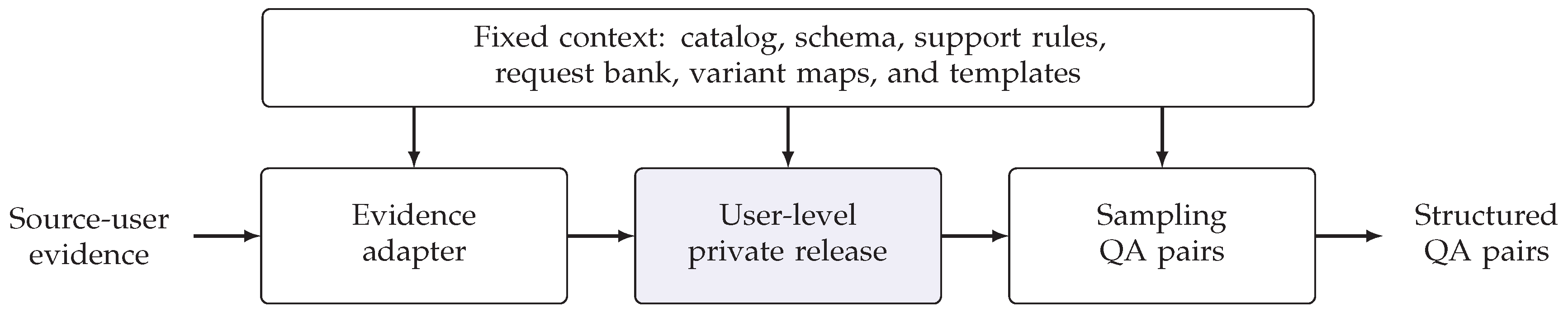
Table 1.
Scope of the user-level privacy guarantee in each domain. Fixed resources are identical in neighboring datasets.
Table 1.
Scope of the user-level privacy guarantee in each domain. Fixed resources are identical in neighboring datasets.
| Property | Movie | Beauty | Recipe |
|---|---|---|---|
| Protected input | Supplied rating history | Each user’s saved review judgments | |
| Supported object | One- to three-tag preference constraint core | One- to three-tag core supported within one review | |
| Requests sharing a count | Same preference constraint core | ||
| Fixed resources | Movie catalog and request-bank rules | Product catalog, normalization, population selection, and request-bank rules | RecipeADQA tag schema and classifier, recipe catalog, and request-bank rules |
| Not covered | Catalog construction and additional unprotected releases | Re-running global 5-core selection after deletion; catalog construction | Raw-review extraction, model-generated labels, aspect-direction selection, and resource construction |
Table 2.
Construction settings of the three datasets.
| Dimension | Movie | Beauty | Recipe |
|---|---|---|---|
| Aspect-direction provenance | Pre-provided metadata | Pre-provided metadata + rule-based cleaning | LLM+SLM inference |
| Evidence for core support | Ratings of matching items | Inferred review judgments of support or opposition | |
| Auxiliary constraints | Optional catalog-attribute constraint | Optional catalog tag and ingredient inclusion or exclusion | |
Table 3.
User populations, request banks, and test set of each dataset. Retained variants are counted before training holdout (Section 5.3), and training records and constraint sets after it.
Table 3.
User populations, request banks, and test set of each dataset. Retained variants are counted before training holdout (Section 5.3), and training records and constraint sets after it.
| Quantity | Bank | Movie | Beauty | Recipe |
|---|---|---|---|---|
| Construction users | 100,394 | 364,798 | 135,783 | |
| Reference users | 5,000 | 5,000 | 5,000 | |
| Support units | Main | 1,021 | 1,021 | 1,024 |
| Random | 1,021 | 1,017 | 850 | |
| Request variants | Main | 3,688 | 3,867 | 4,060 |
| Random | 4,011 | 2,821 | 3,400 | |
| DP-retained variants | Main | 3,265 | 1,698 | 1,390 |
| Random | 1,820 | 36 | 960 | |
| DP training records | Main | 2,758 | 1,463 | 1,158 |
| Random | 1,807 | 36 | 959 | |
| DP distinct constraint sets | Main | 2,424 | 1,356 | 1,019 |
| Random | 1,770 | 36 | 959 | |
| Test / validation questions | 400 / 40 | 400 / 40 | 400 / 40 | |
| Candidates per test question | 30 | 30 | 30 | |
| Constraints per test question | 1–4 | 2–4 | 1–4 | |
| Answers per test question | 2–25 | 2–25 | 1–25 | |
| Mean answers per test question | 17.56 | 17.13 | 16.54 |
Table 4.
Example test requests. The test template renders each constraint set as “I am looking for movies (products, recipes) with the following combination: …. Return all matches.”
Table 4.
Example test requests. The test template renders each constraint set as “I am looking for movies (products, recipes) with the following combination: …. Return all matches.”
| Domain | Preference constraint core | Auxiliary constraints | Answers |
|---|---|---|---|
| Movie | genre::mystery; language::en; runtime::short | era::1920s | 12 |
| Beauty | item_form::spray; scent::sandalwood; scent::vanilla | scent::coconut | 19 |
| Recipe | health::nutrient-dense | convenience::quick; exclusion of the ingredient spinach | 20 |
Table 5.
Test-set macro F1 and EM, in percent.
| Source | Movie | Beauty | Recipe | |||
|---|---|---|---|---|---|---|
| F1 | EM | F1 | EM | F1 | EM | |
| DP | 99.60 | 89.00 | 92.95 | 55.00 | 96.37 | 59.75 |
| Bounded | 99.83 | 96.00 | 97.79 | 76.75 | 95.70 | 59.00 |
| NP | 99.59 | 89.25 | 95.26 | 62.75 | 96.45 | 62.25 |
| Public | 98.81 | 87.75 | 98.92 | 92.25 | 96.73 | 83.25 |
| random DP | 99.38 | 85.25 | 88.02 | 18.50 | 76.74 | 7.75 |
| random Bounded | 97.50 | 60.75 | 94.79 | 51.50 | 86.28 | 11.75 |
| random NP | 98.87 | 75.50 | 94.52 | 44.00 | 69.79 | 7.50 |
| random Public | 99.81 | 96.00 | 99.14 | 83.75 | 50.24 | 6.00 |
| Base | 3.71 | 0.00 | 0.00 | 0.00 | 0.00 | 0.00 |
Table 6.
Paired differences between main DP and the listed source in macro F1 and EM, in percentage points, with 95% paired bootstrap intervals (Section 6.1.2).
Table 6.
Paired differences between main DP and the listed source in macro F1 and EM, in percentage points, with 95% paired bootstrap intervals (Section 6.1.2).
| Domain | DP minus | F1 | F1 interval | EM | EM interval |
|---|---|---|---|---|---|
| Movie | Bounded | -0.24 | [-0.37, -0.10] | -7.00 | [-10.50, -3.75] |
| NP | +0.01 | [-0.18, +0.20] | -0.25 | [-4.29, +3.48] | |
| Public | +0.79 | [+0.25, +1.46] | +1.25 | [-3.19, +5.41] | |
| random DP | +0.22 | [+0.03, +0.42] | +3.75 | [-0.49, +7.96] | |
| Beauty | Bounded | -4.83 | [-6.02, -3.70] | -21.75 | [-26.75, -16.50] |
| NP | -2.31 | [-3.33, -1.23] | -7.75 | [-13.07, -2.49] | |
| Public | -5.97 | [-7.20, -4.81] | -37.25 | [-42.39, -32.17] | |
| random DP | +4.93 | [+3.60, +6.25] | +36.50 | [+30.92, +41.90] | |
| Recipe | Bounded | +0.67 | [-0.74, +2.01] | +0.75 | [-4.53, +6.17] |
| NP | -0.08 | [-1.47, +1.31] | -2.50 | [-8.25, +3.27] | |
| Public | -0.36 | [-1.44, +0.90] | -23.50 | [-28.57, -18.55] | |
| random DP | +19.63 | [+17.60, +21.56] | +52.00 | [+46.56, +57.25] |
Table 7.
Fidelity measures for the main bank before training holdout; user and mass coverage are percentages, and TV is measured to the raw reference target.
Table 7.
Fidelity measures for the main bank before training holdout; user and mass coverage are percentages, and TV is measured to the raw reference target.
| Domain | Source | User coverage | Mass coverage | TV |
|---|---|---|---|---|
| Movie | DP | 95.46 | 99.73 | 0.1273 |
| Bounded | 95.46 | 100.00 | 0.1161 | |
| NP | 95.46 | 100.00 | 0.0076 | |
| Public | 95.46 | 100.00 | 0.4060 | |
| Beauty | DP | 25.42 | 96.43 | 0.1459 |
| Bounded | 25.56 | 100.00 | 0.1327 | |
| NP | 25.56 | 100.00 | 0.1433 | |
| Public | 25.56 | 100.00 | 0.6875 | |
| Recipe | DP | 72.16 | 98.24 | 0.1135 |
| Bounded | 72.24 | 100.00 | 0.0874 | |
| NP | 72.24 | 100.00 | 0.0442 | |
| Public | 72.24 | 100.00 | 0.7284 |
Table 8.
Preference-weighted test set: macro F1 and EM, in percent, with 95% paired bootstrap intervals for F1; the last column repeats each model’s test-set F1.
Table 8.
Preference-weighted test set: macro F1 and EM, in percent, with 95% paired bootstrap intervals for F1; the last column repeats each model’s test-set F1.
| Domain | Source | F1 | F1 interval | EM | Test-set F1 |
|---|---|---|---|---|---|
| Movie | DP | 98.18 | [97.14, 99.05] | 89.94 | 99.60 |
| Bounded | 98.37 | [97.44, 99.21] | 92.53 | 99.83 | |
| NP | 98.37 | [97.60, 98.94] | 83.05 | 99.59 | |
| Public | 96.90 | [96.01, 97.70] | 74.14 | 98.81 | |
| Beauty | DP | 97.82 | [96.82, 98.74] | 88.10 | 92.95 |
| Bounded | 98.99 | [98.45, 99.45] | 87.34 | 97.79 | |
| NP | 98.33 | [97.38, 99.11] | 85.82 | 95.26 | |
| Public | 99.36 | [98.61, 99.86] | 95.70 | 98.92 | |
| Recipe | DP | 93.82 | [91.84, 95.56] | 66.93 | 96.37 |
| Bounded | 97.26 | [96.17, 98.21] | 75.71 | 95.70 | |
| NP | 94.05 | [92.29, 95.71] | 63.57 | 96.45 | |
| Public | 93.86 | [91.96, 95.67] | 77.52 | 96.73 |
Table 9.
Primary attack on the main-bank releases at a 1% FPR target. Public releases give every target the same score, so no target is flagged.
Table 9.
Primary attack on the main-bank releases at a 1% FPR target. Public releases give every target the same score, so no target is flagged.
| Domain | Release | AUC | TPR (%) | FPR (%) | TP | FP |
|---|---|---|---|---|---|---|
| Movie | DP | 0.506 | 0.82 | 0.86 | 41 | 43 |
| Bounded | 0.517 | 1.02 | 0.78 | 51 | 39 | |
| NP | 0.516 | 0.96 | 0.80 | 48 | 40 | |
| Public | 0.500 | 0.00 | 0.00 | 0 | 0 | |
| Beauty | DP | 0.487 | 1.14 | 1.16 | 57 | 58 |
| Bounded | 0.515 | 1.46 | 0.82 | 73 | 41 | |
| NP | 0.515 | 1.36 | 0.74 | 68 | 37 | |
| Public | 0.500 | 0.00 | 0.00 | 0 | 0 | |
| Recipe | DP | 0.504 | 1.10 | 1.24 | 55 | 62 |
| Bounded | 0.533 | 2.12 | 1.38 | 106 | 69 | |
| NP | 0.524 | 1.74 | 1.52 | 87 | 76 | |
| Public | 0.500 | 0.00 | 0.00 | 0 | 0 |
Table 10.
Likelihood-ratio membership attacks on the main-bank target releases at a 1% FPR target. For DP and Bounded, the realistic adversary receives the unthresholded noisy vector and the bounded counts instead of the C+weight views.
Table 10.
Likelihood-ratio membership attacks on the main-bank target releases at a 1% FPR target. For DP and Bounded, the realistic adversary receives the unthresholded noisy vector and the bounded counts instead of the C+weight views.
| Realistic | Informed | ||||
|---|---|---|---|---|---|
| Domain | Release | AUC | TP/FP | AUC | TP/FP |
| Movie | DP unthresholded | 0.518 | 46/43 | 0.617 | 151/51 |
| DP C+weight | – | – | 0.559 | 74/54 | |
| DP C-only | 0.501 | 41/46 | 0.512 | 75/58 | |
| Bounded | 0.518 | 47/41 | 0.999 | 4,788/0 | |
| NP C+weight | 0.517 | 47/50 | 0.999 | 4,788/0 | |
| Beauty | DP unthresholded | 0.505 | 51/22 | 0.527 | 74/37 |
| DP C+weight | – | – | 0.523 | 73/35 | |
| DP C-only | 0.505 | 56/34 | 0.508 | 57/46 | |
| Bounded | 0.506 | 55/27 | 0.715 | 1,267/0 | |
| NP C+weight | 0.505 | 53/26 | 0.715 | 1,267/0 | |
| Recipe | DP unthresholded | 0.502 | 57/61 | 0.537 | 109/44 |
| DP C+weight | – | – | 0.537 | 79/47 | |
| DP C-only | 0.498 | 53/71 | 0.499 | 47/49 | |
| Bounded | 0.502 | 63/55 | 0.964 | 3,691/0 | |
| NP C+weight | 0.500 | 57/45 | 0.964 | 3,691/0 | |
Table 11.
Synthetic audit of the implemented mechanism, with trials counted per hypothesis.
| Design | k | Loss | Trials | (unthresholded) | (C-only) |
|---|---|---|---|---|---|
| Canary | 1 | 0.2 | 200,000 | 0.188 | 0.178 |
| Canary | 5 | 1.0 | 200,000 | 0.888 | 0.882 |
| Canary | 20 | 4.0 | 1,000,000 | 2.263 | 2.305 |
| Canary | 40 | 4.0 | 200,000 | 1.537 | 1.761 |
| Noise-free control | 20 | ∞ | 200,000 | 10.208 | 10.208 |
| Half-scale control | 20 | 8.0 | 200,000 | 4.435 | 4.199 |
Disclaimer/Publisher’s Note: The statements, opinions and data contained in all publications are solely those of the individual author(s) and contributor(s) and not of MDPI and/or the editor(s). MDPI and/or the editor(s) disclaim responsibility for any injury to people or property resulting from any ideas, methods, instructions or products referred to in the content. |
© 2026 by the authors. Licensee MDPI, Basel, Switzerland. This article is an open access article distributed under the terms and conditions of the Creative Commons Attribution (CC BY) license (http://creativecommons.org/licenses/by/4.0/).
Copyright: This open access article is published under a Creative Commons CC BY 4.0 license, which permit the free download, distribution, and reuse, provided that the author and preprint are cited in any reuse.