

Submitted:
07 November 2026
Posted:
10 November 2026
You are already at the latest version
Abstract
Closed-form solutions simplify the design of thick orthotropic plates, but their accuracy for plates with a free edge is unknown. This study developed one-term closed-form and multi-term series solutions of Alternative 1 Theory, with three-dimensional (3D) constitutive relations, for uniformly loaded rectangular orthotropic plates with a free edge. Ten support combinations, with the free edge parallel or perpendicular to the stiff direction, were analysed in 1,200 cases (E1/E2 = 5–40, a/t = 4–20, b/a = 0.5–3.0). A 3D Ritz solution, with deflections within 0.08% of exact, Lévy-type, and finite element solutions, served as the reference, and the series separated shape error from theory error. The converged series underestimated the 3D deflection by 4–19% at a/t = 4 and by up to 10% at a/t = 20. Its error was largest where the stiff direction spans between a clamped and a simply supported edge; there, it also overestimated the clamped-edge moment by up to 129%. Free-edge orientation governed the response. Plates with the free edge across the stiff direction deflected up to 1,050 times as much as their quarter-turned counterparts, and the one-term solution underestimated their deflection by 11–95% for b/a ≥ 1.0. The one-term formulas were within 10% of 3D elasticity in 319 cases, half of them for four plates with a/t ≤ 5 and b/a ≥ 1.0, partly through a cancellation of shape and theory errors. In thick plates, 3D face stresses at the free edge exceeded the linear values by up to 110%.
Keywords:
Alternative 1 Theory
; orthotropic plate
; free edge
; closed-form solution
; three dimensional elasticity
; shear deformation
1. Introduction
Rectangular plates with one unsupported edge are common in structural practice. Deck overhangs and cantilevering slab bays, balcony and canopy slabs, orthotropic steel decks at an open edge, timber floor panels beside a stairwell, and composite panels at a cut-out are all supported on three sides and free on the fourth. Many of these components are orthotropic, either because the material is orthotropic in nature (such as fibre-reinforced polymer laminae, rolled metals, and engineered timber panels) or because stiffening makes the structure behave orthotropically (such as stiffened steel decks) [1,2,3,4]. Their transverse shear moduli are small compared with the stiffer in-plane modulus. Therefore, shear deformation matters at span–thickness ratios for which an isotropic plate would already behave as a thin plate, and the classical (Kirchhoff) theory loses accuracy [5,6,7]. Because the free edge carries no support, it is usually where the largest deflection occurs and where the serviceability of the plate is decided.
A free edge is also the most demanding boundary for an analytical solution. Its conditions are natural rather than geometric: the normal bending moment and the effective (Kirchhoff) shear force must vanish, and concentrated corner forces arise where the free edge meets a supported edge [8,9]. In shear-deformable plate theories, a boundary layer forms along the edges, with a strength that depends on the edge condition [10], and in three dimensions, a free edge creates local stress states that two-dimensional theories capture only partially [11,12]. Solutions built from assumed shapes face a further difficulty. The deflection function must allow the free edge to deflect and rotate, yet no polynomial shape can satisfy both natural conditions exactly, and the choice of free-edge function significantly influences the accuracy of the result.
For thin plates, including orthotropic plates, accurate analytical solutions with free edges are now available. The symplectic superposition method has produced exact bending solutions for cantilever plates [13], plates with two adjacent free edges [14], completely free plates on elastic foundations [15], and plates supported only at their corners [16,17]. The finite integral transform method has provided solutions for cantilever plates under bending [18], for free orthotropic plates under arbitrary loading [19], for orthotropic plates with two adjacent free edges [20], and for orthotropic plates with opposite rotationally restrained and free edges [21]. However, all of these solutions are based on the classical plate theory. Results for shear-deformable plates are fewer. Tian et al. [22] obtained integral transform solutions for moderately thick plates with all edges free on an elastic foundation. Li et al. [23] derived analytical vibration solutions for thick plates with a free edge, and Mladenović et al. [24] analysed thick plates with partially clamped edges using Reissner’s theory. Exact three-dimensional (3D) elasticity solutions exist for only a few cases. Based on 3D elasticity and on shear deformation theories, Atashipour et al. [25] derived Lévy-type solutions for thick laminated orthotropic plates that may have free edges; however, the Lévy approach requires the two edges that meet the free edge to be simply supported. Revenko [26] presented an exact 3D solution for an orthotropic cantilever loaded at its end, and semi-analytical 3D methods have been applied to thick plates with general supports [27]. Consequently, plates that combine a free edge with clamped adjacent edges, such as the CCFC, CFCS, SFCC, and CFSS plates, have no exact 3D solution. To the best of the authors’ knowledge, no 3D reference values have been reported for orthotropic plates of these types.
Closed-form solutions from refined plate theories fill part of this gap. A polynomial shear deformation theory has been applied to isotropic thick plates with three clamped edges and one free edge [28], and Alternative I refined plate theory to isotropic plates with clamped and free edges [29]. A recent review of thick-plate research found that most studies concern plates whose edges are all simply supported or all clamped, and it called for work on other combinations, including plates with a free edge [30]. The available refined-theory solutions share three limitations. Each uses a single assumed shape whose error is never separated from the error of the theory. Their accuracy has seldom been measured against 3D elasticity and, to the authors’ knowledge, never for orthotropic plates with a free edge and clamped adjacent edges. Finally, they do not consider whether the free edge runs along or across the stiff material direction, although this decides how the load is carried in an orthotropic plate.
Alternative 1 Theory [31] offers a convenient basis for closed-form solutions of shear-deformable plates. Its in-plane displacements are single quantities that vary linearly through the thickness, and each rotation is related to the slope of the deflection in its own plane by a ratio found from energy minimisation. Thus, the shear strains follow from the kinematics, and no shear correction factor is required [29,31]. The theory has been combined with 3D constitutive relations for isotropic plates [29]. Its assumptions have also been built into a modified first-order theory for thick anisotropic plates [32], while the related Alternative II theory has been applied to the 3D bending and buckling of anisotropic plates [33]. For a free edge, the strip functions of the theory add a fifth-degree term and close the shape with an extra slope relation at the free edge [31]. How well such a closed shape represents an orthotropic plate with a free edge, and whether the remaining error lies in the shape or in the theory, has not been established. Consequently, designers of thick orthotropic plates with a free edge lack deflection and moment formulas of known accuracy. The existing solutions provide neither a measure of their error nor 3D reference values for most support combinations.
This study aimed to develop closed-form and multi-term Alternative 1 Theory solutions for uniformly loaded rectangular orthotropic plates with a free edge and to determine when they can be used. Ten plates were analysed. In six of them (SSFS, CCFC, CCFS, SSFC, SCFC, and CSFS), the free edge runs parallel to the stiff direction, whereas in the other four (SFSC, CFCS, SFCC, and CFSS), the free edge runs across the stiff direction. Four modular ratios, five span–thickness ratios from 4 to 20, and six aspect ratios from 0.5 to 3.0 were considered. A multi-term Legendre series whose first term is the closed form separated the error of the one-term shape from that of the theory, and a Ritz solution of 3D elasticity [34], validated against exact, Lévy-type, and finite element solutions, provided the reference.
This study extends existing research in four distinct ways. First, it gives explicit one-term formulas for ten orthotropic plates with a free edge. The formulas include reflected free-edge functions for a free edge across the stiff direction and a Poisson-coupling integral that no longer equals its symmetric counterpart when an edge is free. Second, it provides validated 3D benchmark deflections and moments for seven plates that have no exact solution. Third, by separating the shape error from the theory error, it explains why the one-term solution fails when the free edge crosses the stiff direction. It also identifies the clamped–simply supported span as the source of the largest theory errors and of a large overestimation of the clamped-edge moments. Fourth, it maps the span–thickness and aspect ratios for which the one-term formulas are adequate for preliminary design, and it quantifies the non-linear through-thickness stresses that a theory with linear in-plane displacements cannot represent.
2. Theoretical Formulation
The ten plates treated in this paper share one displacement field, one energy functional, and one set of stress-recovery formulas. They differ only in the one-dimensional edge functions from which the deflection surface is built. Therefore, the plate is formulated once, in Section 2.1, Section 2.2, Section 2.3 and Section 2.4, and the edge conditions are included only in Section 2.5 and Section 2.6. The kinematic and constitutive framework is that of Alternative 1 Theory in its 3D form. Four elements are specific to plates with a free edge and are developed here. They are (i) the argument that fixes the through-thickness variation of the deflection when one edge carries no support and (ii) the quintic edge functions of strips with a free end, with their reflected forms for a free edge on x = 0. The other two are (iii) the Poisson-coupling integral, which no longer equals its symmetric counterpart once an edge is free, and (iv) the natural conditions of the free edge, which are not imposed but are measured after the solution has been obtained.
2.1. Geometry, Edge Numbering, and Plate Designation
Consider a rectangular plate of length a, width b, and uniform thickness t, made of a homogeneous orthotropic material (Figure 1). The Cartesian origin is placed at the top left corner of the middle surface in plan (Figure 1a). The x-axis runs to the right along the top edge, the y-axis runs downward along the left edge, and the z-axis is directed downward through the thickness (Figure 1b). The principal material axes coincide with x, y, and z, and the largest Young’s modulus, E1, acts in the x-direction. A uniformly distributed transverse load of intensity q is applied to the upper face, z = −t/2.
The edges are numbered as follows: edge 1 (y = 0, top), edge 2 (x = 0, left), edge 3 (y = b, bottom), and edge 4 (x = a, right). A plate is designated by four letters giving the conditions of edges 1 to 4 in that order, where S denotes a simply supported edge, C denotes a clamped edge, and F represents a free edge. In six of the plates (SSFS, CCFC, CCFS, SSFC, SCFC, and CSFS), edge 3 is free and runs parallel to the stiff direction. In the other four (SFSC, CFCS, SFCC, and CFSS), edge 2 is free, and the free edge runs across the stiff direction. The material axes are fixed to the plate and do not turn with the supports. Hence, a plate of the second group is not a rotated copy of any plate in the first, even when its supports match up to a quarter turn.
The non-dimensional coordinates and plate ratios are defined as follows:
where ∝ is the span–thickness ratio, and β is the aspect ratio. Note that 0 ≤ X, Y ≤ 1, −1/2 ≤ Z ≤ 1/2, and the load acts on the face Z = −1/2.
2.2. Kinematics
2.2.1. Displacement field
Alternative 1 Theory [29,31] rests on three assumptions. The middle surface does not stretch, and a straight transverse fibre remains straight but may tilt relative to the normal of the deformed middle surface. In addition, each in-plane displacement is a single quantity proportional to z, and the displacements are written as follows:
where θx and θy are the rotations of the transverse fibre in the xz- and yz-planes, respectively. No form is imposed on the variation of w with z at this stage; it is fixed in Section 2.2.3.
u = z θx(x,y), v = z θy(x,y), w = w(x,y,z)
The defining relation of the theory links each rotation to the slope of the deflection in its plane through a rotation–slope ratio:
The ratios Cx and Cy are not prescribed; they are unknowns to be found by minimising the total potential energy (Section 2.8). In a thin plate, both approach −1, the fibre stays normal to the middle surface, and the Kirchhoff kinematics are recovered.
2.2.2. Strain Components
The small-strain relations of 3D elasticity applied to Eq. (2), with the coordinates of Eq. (1), yield the in-plane strains, which vary linearly through the depth:
and the transverse strains are expressed as follows.
With Eq. (3), the transverse shear strains become γxz = (1 + Cx)∂w/∂x and γyz = (1 + Cy)∂w/∂y. They follow directly from the assumed displacements, and the transverse shear stresses follow from them through Hooke’s law. For this reason, no shear correction factor is introduced.
2.2.3. Through-Thickness Variation of the Deflection
Because θx and θy in Eq. (2) do not depend on z, differentiating Eq. (3) with respect to z, with Cx and Cy non-zero, gives
Hence, the deflection must take the form w = w0(X, Y) + f(Z). The function f(Z) is the same at every point of the plan. For plates whose four edges are supported, f is removed because w vanishes over the depth of every edge. That argument cannot be applied edge by edge for the plates analysed in this study because the free edge places no restriction on w. However, it is sufficient for w to vanish over the depth of a single supported edge: on such an edge, w0 + f(Z) = 0 for every Z, which can only hold if f is a constant, and the constant is absorbed into w0. Because each of the ten plates has three supported edges, it follows that
w = w(X,Y), εz = 0.
Thus, the transverse normal strain disappears from the formulation, although, as Section 2.3 shows, the 3D constitutive coefficients do not.
2.3. Constitutive Relations
2.3.1. Three-Dimensional Stiffness Coefficients
All six stress components are retained. For an orthotropic material with principal axes along x, y, and z, the stiffness form of Hooke’s law is written with a reference modulus E0 as follows.
In this paper, E0 = E2. The dimensionless coefficients are expressed in terms of the nine independent elastic constants:
where the minor Poisson’s ratios follow from the symmetry of the compliance matrix, μij/Ei = μji/Ej. The material used throughout is of the Pagano type, with E2 = E3, G12 = G13 = 0.5E2, G23 = 0.2E2, and μ12 = μ13 = μ23 = 0.25. Four modular ratios, E1/E2 = 5, 10, 25, and 40, are considered. The resulting coefficients are listed in Table 1.
Δ=1 − μ12μ21 − μ23μ32 − μ13μ31 − 2μ21μ32μ13
2.3.2. Reduced Coefficients
Because εz = 0 by Eq. (7), only c11, c12, c22, c44, c55, and c66 enter the strain energy, and they enter with their full 3D values. Plate theories more commonly take σz = 0 instead [7]. Eliminating εz from Eq. (8) under that condition gives the reduced (plane-stress) coefficients:
with c44, c55, and c66 unchanged. Both coefficient sets were used for analysis in this study. The full set of Eq. (9) is used in the equations as written, and the reduced variant is obtained by replacing c11, c12, and c22 with , , and , respectively, in every equation from Eq. (12) onward. For the present materials, the reduction lowers c11 by 0.3–2%, c22 by 6–7%, and c12 by 25–27% (Table 1). Therefore, its effect on the response is largest where the plate bends mainly in the y-direction, which, as shown later, is the case near a free edge that runs across the stiff direction.
2.4. Total Potential Energy
The strain energy is , and the potential of the load is evaluated on the loaded face. Substituting Eqs. (4), (5), (7), and (8) and integrating through the depth with gives the total potential energy, Π = U − V, as a double integral over the unit square:
where D0 = E0t3/(12Δ) is the reference flexural rigidity. The first integral is the bending energy, and the second is the transverse shear energy. The factor ∝2 in front of the second integral increases rapidly as the plate becomes thinner. Consequently, the shear strains must become small, and Cx and Cy must approach −1.
2.5. Boundary Conditions
2.5.1. Supported Edges
On an edge with outward normal n, the conditions are as follows:
By Eq. (3), a zero slope normal to a clamped edge also makes the normal rotation zero at that edge. The conditions w = 0 and ∂w/∂n = 0 are geometric (essential) conditions, and every trial function used below satisfies them exactly. The zero-curvature condition of the simple support is a natural condition in the energy method. Nevertheless, it is built into the one-term edge functions, as is customary for polynomial shapes.
2.5.2. Free Edge
A free edge carries no traction. In the Kirchhoff form, which has two conditions per edge and which the theory approaches as ∝ → ∞, the normal bending moment and the effective (Kirchhoff) shear force must vanish [8]. On edge 3 (Y = 1) and on edge 2 (X = 0), these conditions are written, in the non-dimensional resultants of Section 2.9, as follows:
At a corner where the free edge meets a supported edge, the abrupt change in twisting moment generates a concentrated corner force, so Vn cannot vanish in the immediate neighbourhood of the corner in any smooth solution [8]. Both conditions are natural conditions of Eq. (12): they are not imposed on the trial functions but are satisfied only as the solution converges. Therefore, they are used in this paper as a measure of accuracy (Section 2.9.4) rather than as constraints.
2.6. Displacement Functions
2.6.1. Product Form And Supported Strips
The deflection is built as a product of two one-dimensional edge functions, each of which describes a strip of the plate spanning between two opposite edges:
h1(X,Y) = gx(X) gy(Y)
The function gx is determined by the conditions of edges 2 and 4, and gy by those of edges 1 and 3. For a strip whose two ends are supported, Eq. (13) applied at s = 0 and s = 1, where s represents X or Y, gives the following quartic functions:
where the first letter of a subscript refers to the end s = 0. The strip that is simply supported at s = 0 and clamped at s = 1 is the reflection .
2.6.2. Strips with a free end
Let r be a local coordinate that runs from the supported end of a strip (r = 0) to its free end (r = 1). At the free end, the strip analogues of Eqs. (14) and (15) are zero curvature and zero third derivative, d2g/dr2 = d3g/dr3 = 0. Together with the two conditions at the supported end, these give four conditions. For a strip that is simply supported at r = 0, the only quartic that satisfies all four is the rigid rotation g = r, which cannot describe bending. Therefore, a fifth-degree term is added, and, for consistency, the strip that is clamped at r = 0 is given the same degree. For a strip that is simply supported at r = 0, the conditions g(0) = d2g/dr2(0) = 0 and d2g/dr2(1) = d3g/dr3(1) = 0 leave the one-parameter family
and, for a strip that is clamped at r = 0, the conditions g(0) = dg/dr(0) = 0 and d2g/dr2(1) = d3g/dr3(1) = 0 leave
which, for a5 = 0, contains the quartic (6r2 − 4r3 + r4)/6 of a uniformly loaded cantilever strip.
The remaining parameter is fixed by an additional relation between the slope at the free end and the coefficient of the fifth-degree term. Following the procedure of Ibearugbulem [31] for strips with a free end, this relation is dg/dr(1) = −(2/3)λ in Eq. (18), and dg/dr(1) = −(1/5)a5 in Eq. (19). These relations give λ = −3/7 and a5 = −5/14, and the edge functions become
The slope relation is a closing assumption of the one-term shape and does not follow from the plate equations. Its consequences are examined through the multi-term series of Section 2.6.4, which does not use it.
When edge 3 is free, r = Y, and gy(Y) = gSF(Y) or gCF(Y). When edge 2 is free, the free end lies at X = 0, so r = 1 − X, and the reflected functions are
Because the outward normal of edge 2 points in the −x direction, d/dn = −d/dX on that edge. When the slope relation is stated in r, as above, it holds with the same coefficients for both free-edge positions, and the reflection preserves all four end conditions. Table 2 summarises the edge functions of the ten plates.
2.6.3. Rotations
In line with Eq. (3), the rotations of the one-term solution are proportional to the slopes of h1:
where A1, A2, and A3 are amplitudes, and Cx = A2/A1 and Cy = A3/A1. No condition is placed on the rotations at the free edge.
2.6.4. Multi-Term Legendre Series
To separate the error of the one-term shape from that of the theory, the one-term shape is improved using shifted Legendre polynomials:
hmn(X,Y) = h1(X,Y) Pm(2X − 1) Pn(2Y − 1), m = 0,1,…,M − 1; n = 0,1,…,N − 1
where Pm is the Legendre polynomial of degree m. The first term (m = n = 0) is the one-term solution, so the series reduces to Eq. (22) when M = N = 1. Each term carries its three amplitudes, and the ratios A2,mn/A1,mn and A3,mn/A1,mn act as term-wise rotation–slope ratios. Every hmn contains h1 as a factor and, thus, satisfies the geometric conditions of the supported edges. However, multiplication by Pm or Pn alters the derivatives of h1 at the free end. Therefore, the higher terms do not inherit the free-end conditions or the slope relation of Section 2.6.2, and the series is free to approach the natural conditions of Eqs. (14) and (15) through the energy minimisation. Where gx or gy is symmetric about the mid-span (Table 2), only even degrees are retained in that direction.
2.7. Governing Equations
Substituting Eq. (24) into Eq. (12) and setting the derivatives of Π with respect to every amplitude to zero gives a symmetric linear system of order 3K, where K is the number of retained terms:
where are the non-dimensional amplitudes. The blocks are defined as
The entries of the stiffness and load arrays are integrals over the unit square of products of the shape functions and their derivatives:
where i and j run over the K retained terms. Because each hi is a product of a function of X and a function of Y, every integral factorises into two single-variable polynomial integrals, which are evaluated exactly.
For plates supported on all four edges, integration by parts shows that k′xy = kxy, and the Poisson and twisting couplings can be combined. With a free edge, this equality no longer holds. For the strip function g in the direction normal to the free edge,
and the boundary term does not vanish because both the deflection and slope are non-zero at the free end. Consequently, k′xy ≠ kxy, and the two integrals are kept separate in Eq. (26). Combining them would introduce an error into the coupling between the two bending directions. K23 is not symmetric in i and j, but the complete matrix of Eq. (25) is, because K23 and its transpose occupy mirror positions.
For the multi-term series, Eq. (25) is solved numerically. Because the high-degree Legendre terms make the matrix poorly scaled, the system is first equilibrated by symmetric diagonal scaling. The series was truncated at Legendre degree 31 in each direction for the CCFC, CCFS, SCFC, CFCS, SFCC, and CFSS plates and at degree 23 for the SSFS, SSFC, CSFS, and SFSC plates, with only even degrees in a direction of symmetry. Convergence was confirmed by repeating each case with eight additional degrees.
2.8. One-Term Closed-Form Solution
2.8.1. Rotation–Slope Ratios
For K = 1, Eq. (25) has three unknowns. Dividing the second and third equations by gives two linear equations for the rotation–slope ratios:
with the solution
d11Cx + d12Cy = d13, d12Cx + d22Cy = d23
Dividing the integrals of Eq. (27) for h1 by kxy reduces them to seven rational constants that depend only on the supports of a plate. These are λ1 = kx/kxy, λ2 = 12kxz/kxy, λ3 = ky/kxy, λ4 = 12kyz/kxy, λ5 = kh/kxy, λ6 = 1200h1(X0, Y0), and λ7 = k′xy/kxy. The coefficients of Eq. (29) are then expressed as
For the free-edge plates, λ7 < 1 (Table 3), which reduces the Poisson coupling d12 relative to that of a plate with all edges supported.
2.8.2. Deflection Amplitude and Deflection
The first equation of Eq. (25) contains the transverse shear terms multiplied by ∝2. Subtracting the second and third equations from the first cancels these terms because K11 = K12 + K13, and directly yields the amplitude:
This form avoids multiplying a large ∝2 by a small (1 + C), which would otherwise cause a loss of precision in thin plates. The one-term deflection at the evaluation point of Table 2 is
2.8.3. Constants of the Ten Plates
Table 3 lists the exact constants. Plates related by a quarter turn of their supports (SSFC and CFSS, CCFS and SFCC, SCFC and CFCS, and CSFS and SFSC) share λ5, λ6, and λ7, and have λ1 interchanged with λ3 and λ2 with λ4. They remain different problems because c11 ≠ c22 and c55 ≠ c44, and because the free edge of the second plate in each pair crosses the stiff direction instead of running along it. SSFS and CCFC have no such counterpart among the ten plates.
2.9. Displacements, Stress Resultants, and Stresses
The expressions in this section are written for the K-term series. For the one-term solution, K = 1, , and .
2.9.1. Displacements, Moments, and In-Plane Stresses
The non-dimensional displacements are as follows:
The bending and twisting moments per unit width, , , and , are
and the in-plane stresses vary linearly through the depth:
The stresses on the faces, at Z = ±1/2, are reported at two locations. These are the midpoint of the free edge, where the moment parallel to the edge acts, and the midpoints of the clamped edges, where the normal moment typically governs design.
2.9.2. Shear Forces and Transverse Shear Stresses
The constitutive shear force, which is proportional to (1 + C) times the slope, vanishes wherever the slope vanishes, including along a clamped edge where the true shear force is greatest. Therefore, the shear forces are recovered from moment equilibrium, Qx = ∂Mx/∂x + ∂Mxy/∂y and Qy = ∂Mxy/∂x + ∂My/∂y:
Integrating the first two equilibrium equations of 3D elasticity through the depth, with zero shear traction on both faces, yields parabolic transverse shear stresses:
2.9.3. Transverse Normal Stress
The third equation of equilibrium, ∂τxz/∂x + ∂τyz/∂y + ∂σz/∂z = 0, is integrated from the unloaded face, Z = 1/2, where σz = 0, to give
The factor, G = −(1/q)(∂Qx/∂x + ∂Qy/∂y), measures how closely the solution satisfies vertical equilibrium at a point. An exact solution has G = 1, which gives σz = −q on the loaded face. Because the energy method enforces equilibrium only in an integral sense, G is computed from Eq. (39) and is reported as obtained, not set to unity. Its departure from 1 is a pointwise check on the solution. The constitutive value of σz expressed by Eq. (8) with εz = 0 is the stress that maintains εz = 0, not the normal stress transmitted through the depth, so it is not used.
2.9.4. Residuals of the Free-Edge Conditions
The natural conditions of Eqs. (14) and (15) are evaluated along the free edge after the solution has been obtained. The moment residual is defined as the largest value of on the free edge divided by the largest value of over the plate. The shear residual is defined as the largest value of on the free edge divided by the largest value of over the plate. Here, n = y for edge 3, and n = x for edge 2. Near the corners, cannot vanish, even in an exact solution, because a concentrated corner force acts there (Section 2.5.2). Therefore, both residuals are reported over the central 80% of the edge, which excludes 10% at each end, and over the whole edge. Only the central-80% residuals approach zero as the solution converges, so they show how well a given shape represents the free edge.
2.10. Three-Dimensional Reference Solutions
2.10.1. Ritz Solution of Three-Dimensional Elasticity
No exact 3D solution is available for most of the ten plates. Therefore, the reference is a Ritz solution of 3D elasticity of the type used for thick plates in [34]. Each displacement component is expanded as a triple product of Legendre polynomials in x, y, and z, multiplied by edge factors that enforce the geometric conditions. On a clamped edge, u = v = w = 0 over the full depth. On a simply supported edge, the support is of the hard type: w and the displacement tangential to the edge vanish over the full depth, and the normal displacement is free [35]. On the free edge, no factor is applied to any component, so the traction-free condition is left as a natural condition of the 3D energy. The stiffness matrix of Eq. (8) is used without any assumption on εz or σz, and the load q is applied to the face z = −t/2. Between 10 and 21 polynomials were used along x and between 13 and 24 along y, depending on the aspect ratio, and 10 through the thickness, giving 5,760–8,190 unknowns (Section 3.2). The moments and face stresses of the reference solution are obtained by integrating the 3D stresses through the depth. Where the free edge meets a clamped edge, the 3D stresses are singular at the corner. Hence, the local stresses near such corners converge slowly, whereas the deflection and the mid-edge stresses are not affected.
2.10.2. Lévy-Type Solution of Three-Dimensional Elasticity
Three of the plates, SSFS, CSFS, and SFSC, have a pair of opposite edges that are simply supported. For these, a semi-analytical 3D solution is also constructed in the manner of the Lévy-type 3D solutions in [25]. Let ξ denote the coordinate normal to the simply supported pair, measured as a fraction of its span (ξ = X for SSFS and CSFS, and ξ = Y for SFSC). The displacement component along ξ is expanded in cos(mπξ), and the other two in sin(mπξ). With these expansions, the hard simple-support conditions are satisfied exactly, and the harmonics uncouple because the material axes are aligned with the plate. The load is expanded as over odd m. For each harmonic, the dependence on the remaining in-plane coordinate and on z is represented by a Legendre Ritz expansion of 22 × 8 polynomials per displacement component. Edge factors are applied only at the supported or clamped end, and 41 odd harmonics are summed. This solution is independent of the 3D Ritz solution in its treatment of one in-plane direction and is used to validate the Ritz reference at the free edge (Section 3).
2.10.3. Error Measures
The error of the one-term closed form relative to 3D elasticity is split into two parts. The shape error, εs = w1/wK − 1, compares the one-term deflection with the converged series. It measures the error caused by the one-term shape alone, under the same theory. The theory error, εt = wK/w3D − 1, compares the converged series with the 3D reference and measures the error of the kinematic assumptions of Alternative 1 Theory. The total error is w1/w3D − 1 = (1 + εs)(1 + εt) − 1. Both measures are evaluated for the maximum deflection, which is located on the computed surface of each solution, and for the deflection at the midpoint of the free edge.
3. Convergence and Validation
Before the parametric results are used, three questions must be answered. First, has the multi-term series converged well enough for the shape error and the theory error to be separated cleanly? Second, has the 3D reference converged, and does it agree with independent solutions, including at the free edge? Third, does the formulation of Section 2 reproduce exact results where they exist? These questions are treated in turn in Section 3.1 to 3.4, and the resulting accuracy of each solution is summarised in Section 3.5. Unless stated otherwise, the full coefficients of Eq. (9) are used.
3.1. Convergence of the Multi-Term Series
3.1.1. Deflection, Free-Edge Moment, and Equilibrium Ratio
Table 4 follows four cases as the highest Legendre degree in each direction rises from 0, the one-term closed form, to 39. The cases cover a free edge parallel to the stiff direction (SSFS and CCFC) and across it (SFSC and CFSS), thick and moderately thin plates, and aspect ratios from 1.0 to 3.0. The equilibrium ratio G of Eq. (39) is evaluated at an interior point on the line through the free-edge midpoint, a quarter of the span from the free edge. This point is (X, Y) = (0.5, 0.75) when edge 3 is free and (0.25, 0.5) when edge 2 is free.
The SSFS plate, whose free edge meets two simply supported edges, converges fastest: and the free-edge moment are steady to five digits once the degree reaches 15, and G equals 1.000. Convergence is slowest for the CCFC plate at ∝ = 4, in which both ends of the free edge meet clamped edges. Between degrees 31 and 39, of this plate increases by 0.13% (from 1.6854 to 1.6876), whereas the free-edge moment is already steady to four digits at degree 15. The other cases change by less than 0.01% between degrees 31 and 39. In every case of Table 4, the converged series gives G within 1.1% of unity at the check point. The CFSS plate at β = 3.0, which has the largest deflections in the study, approaches unity more slowly than the others, with G = 1.034, 1.020, and 1.011 at degrees 23, 31, and 39.
The one-term values in Table 4 show the size of the shape error before any comparison with 3D elasticity is made. For the plates whose free edge runs along the stiff direction, the one-term deflection is 9.5% (CCFC) and 23.5% (SSFS) higher than the converged series. For those whose free edge crosses the stiff direction, the one-term deflection is 56% (SFSC) and 95% (CFSS) lower. Moreover, the one-term solution always positions the maximum deflection on the free edge. For the CCFC plate at ∝ = 20 (E1/E2 = 40, β = 1.0; not shown in Table 4), the converged maximum instead lies inside the plate at Y = 0.46 and exceeds the free-edge deflection by 1.0%. The one-term solution also violates local equilibrium: G ranges from −2.52 to 1.13 at the check points of Table 4.
On the basis of these results, the parametric study used degrees up to 31 for the CCFC, CCFS, SCFC, CFCS, SFCC, and CFSS plates and degrees up to 23 for the SSFS, SSFC, CSFS, and SFSC plates (Section 2.7). Each of the 1,200 cases was repeated with eight additional degrees. The largest resulting change in was 0.25% (CCFC, ∝ = 5). The change exceeded 0.1% in 107 of the 1,200 cases, all of them CCFC, CCFS, SSFC, SCFC, or CFCS plates, and the median change did not exceed 0.08% for any plate. The largest variation for each plate is listed in Table 5.
3.1.2. Free-Edge Conditions
Table 5 lists the largest residuals of the free-edge conditions for each plate over the 120 cases of that plate, measured over the central 80% of the free edge as defined in Section 2.9.4. The converged series satisfies both natural conditions closely: the moment residual does not exceed 3.8% (SSFC) and the shear residual does not exceed 2.6% (SSFS). The one-term solution leaves considerably larger residuals: 18.6–100% for the moment and 11.3–46.8% for the effective shear. A moment residual of 100% for the SSFS and CSFS plates indicates that the normal moment on the free edge is as large as the greatest normal moment anywhere in the plate. The one-term strip enforces zero curvature normal to the free edge but leaves the Poisson term c12 ∂2w/∂x2 of , which is significant along a free edge that runs in the stiff direction.
Over the entire edge, including the corners, the series residuals remain equally small for the SSFS, CSFS, and SFSC plates, whose free edge ends at simply supported edges. Where the free edge meets a clamped edge, the whole-edge residuals reach up to 100% for the moment and up to 2.6 times the largest interior shear force for the effective shear. These large values are confined to the immediate neighbourhood of the corner, where the clamped-edge constraint makes a non-zero Poisson moment unavoidable in any smooth trial function and where the concentrated corner force of Section 2.5.2 acts. For this reason, the central-80% residuals are used as the measure of how satisfactorily a solution represents the free edge.
3.2. Convergence of the Three-Dimensional Reference
The convergence of the 3D Ritz solution was examined separately in the plane and through the thickness (Table 6). Two square plates with clamped–free corners and the largest shear effects (CCFC and CFCS, E1/E2 = 40, ∝ = 4) were used, together with a long plate (SFCC, β = 3.0). The through-thickness expansion proved to be the controlling factor. Raising the number of polynomials in z from 6 to 10, with the in-plane expansion unchanged, increases the free-edge deflection of the CCFC plate by 0.29%, that of the CFCS plate by 0.06%, and that of the SFCC plate by 0.03%. By contrast, a further refinement of 20–30% in the plane changes these deflections by no more than 0.014%. The effect of the z-expansion is largest for the thick, strongly orthotropic plates with clamped edges, in which the in-plane displacements near a clamped edge vary through the depth in a way that low-degree polynomials cannot follow. Therefore, the reference solutions of all 1,200 cases were computed with 10 polynomials in z.
With 10 polynomials in z, the in-plane refinement in Table 6 changes the free-edge moment by at most 0.07%, except for the small moment of the SFCC plate (6 ≈ 0.015), which changes by 1.3%. The clamped-edge moments change by at most 0.09%, or by 0.34% at edge 3 of the SFCC plate (not shown). Therefore, the deflections of the 3D reference are converged to approximately four significant digits and its mid-edge moments to within a few tenths of a per cent.
3.3. Validation of the Three-Dimensional Reference
3.3.1. Exact Solution for a Simply Supported Plate
For a plate with all four edges simply supported (hard type), the exact 3D solution can be obtained using Pagano’s method [35]. It was computed here independently, in state-space form, by summing 50 × 50 odd harmonics, which converges the tabulated values to at least five digits. Table 7 compares it with the 3D Ritz solution using the same polynomial numbers as the parametric study. The deflections agree within 0.001%, and the face stresses are in agreement within 0.03%.
3.3.2. Lévy-Type Solutions for Plates with a Free Edge
The SSFS, CSFS, and SFSC plates were checked against the Lévy-type 3D solution of Section 2.10.2 at the free-edge midpoint, the point that matters most for these plates. The comparison covered 240 cases, with E1/E2 = 5, 10, 25, and 40, ∝ = 4, 5, 10, 15, and 20, and β = 0.5, 1.0, 2.0, and 3.0. With 30 × 12 polynomials and 61 harmonics instead of 22 × 8 and 41, its free-edge deflection changed by at most 0.02% and its free-edge moment by at most 0.05%. Across all 240 cases, the free-edge deflection of the Ritz reference agrees with the Lévy-type value within 0.04%, and the free-edge moment is in agreement within 0.004 in absolute terms. Relative to the Lévy-type moment, the difference is at most 0.07% for the SSFS plate and 0.34% for the CSFS plate. For the SFSC plate, it reaches 1.7% at β = 2.0 and ∝ ≥ 10, where the moment parallel to the free edge is small (6 = 0.10–0.22) and the Ritz moment is the lower of the two. Table 8 presents representative values for E1/E2 = 25.
3.3.3. Finite Element Solutions for Plates with Clamped and Free Edges
No exact solution exists for the seven plates that lack a simply supported pair of opposite edges. For these, the Ritz reference was compared with an independent FE model built in CalculiX [36], with 20-node hexahedral elements and reduced integration (C3D20R). The model had the same hard simple supports and clamped faces, a traction-free free edge, and the load applied as a pressure on the face z = −t/2. The FE moments were obtained by integrating the nodal stresses through the thickness at the edge point. The results are included in Table 6. On the finer mesh, the FE deflections are within 0.08% of the Ritz values with the largest polynomial numbers (CCFC, +0.02%; CFCS, −0.08%; SFCC, −0.02%), and they change by at most 0.07% between the two meshes. The clamped mid-edge moments are in agreement within 0.23%. The free-edge moments differ by up to 1.2% (CCFC), and by 0.0012 in absolute terms for the small free-edge moment of the SFCC plate. These differences decrease with mesh refinement and are attributed to the extrapolation of FE stresses to a free surface. The same FE model reproduces the Lévy-type free-edge deflection of the SSFS plate (E1/E2 = 40, ∝ = 4, β = 1.0) to five digits (2.3354 against 2.3354).
3.4. Thin-Plate Limit
As ∝ → ∞, Alternative 1 Theory tends to classical plate theory (CPT), and the SSFS, CSFS, and SFSC plates then have exact Lévy solutions with the free-edge conditions of Eqs. (14) and (15). These solutions were computed with the same stiffness coefficients and 101 harmonics and compared with the series and the one-term solution at ∝ = 10,000 (Table 9). This comparison tests the parts of the formulation that are specific to a free edge, namely the reflected edge functions, the separate Poisson-coupling integral k′xy, and the recovery of the free-edge moment, independently of the 3D reference. For both coefficient sets, the series reproduces the exact deflections within 0.0002% and the exact free-edge moments within 0.017%. The largest relative moment difference occurs where the moment itself is almost zero (SFSC, β = 3.0).
The one-term errors in Table 9 confirm that the shape error is not a thick-plate effect. In the thin limit, the one-term deflection at the free-edge midpoint differs from the exact value by −26.7% to +27.0% for the SSFS and CSFS plates and by −11.8% to −67.0% for the SFSC plate. These errors are similar to the shape errors found for thick plates in Section 3.1.
3.5. Summary of Accuracy
The checks above establish the accuracy of each solution used in Section 4:
- 3D reference: Deflections are converged to approximately four significant digits and agree with the exact SSSS solution within 0.001%, with the Lévy-type solutions within 0.04%, and with the FE solutions within 0.08%. Mid-edge moments are converged to within a few tenths of a per cent.
- Multi-term series: Truncation changes
by at most 0.25%, and the free-edge conditions are satisfied to within 3.8% (moment) and 2.6% (effective shear) away from the corners. In the thin limit, the series reproduces the exact CPT solutions with free edges to better than 0.0002%.
- Shape and theory errors: The series and the 3D reference are both converged to well within 1%. Thus, differences between them larger than approximately 0.3% can be attributed to the kinematic assumptions of the theory (theory error), and differences between the one-term and series solutions to the one-term shape (shape error).
4. Results and Discussion
This section presents the results of the 1,200 cases (ten plates, four modular ratios, five span–thickness ratios, and six aspect ratios). Section 4.1 presents benchmark 3D values. Section 4.2 and Section 4.3 describe how the plates deform and how the orientation of the free edge governs their response. Section 4.4 discusses the error of Alternative 1 Theory (the theory error), and Section 4.5 the accuracy of the one-term closed form (the shape error and the total error). Section 4.6 deals with stresses. Unless stated otherwise, the full coefficients of Eq. (9) are used, and deflections and moments are provided in the non-dimensional forms of Eqs. (34)–(36). The complete results of all 1,200 cases, for both coefficient sets, are provided as Supplementary Material.
4.1. Benchmark Three-Dimensional Results
Table 10 and Table 11 list the 3D reference deflections and moments for E1/E2 = 25 and β = 1.0 at three span–thickness ratios, together with the corresponding series and one-term values. Because no exact solution exists for seven of the ten plates, and the 3D values were validated in Section 3 to about four significant digits for the deflection, these values may serve as benchmarks for other plate theories.
The free edge dominates the response. In 1,121 of the 1,200 cases, the maximum deflection occurs on the free edge; the exceptions are discussed in Section 4.2.2. Plates whose free edge crosses the stiff direction (SFSC, CFCS, SFCC, and CFSS) deflect much more than those whose free edge runs along it, with = 4.28–8.37 for the former and 0.42–0.97 for the latter at ∝ = 10 (Table 10). In the SFCC and CFSS plates, the maximum lies on the free edge but away from its midpoint (Y = 0.43–0.57), because the supports at its two ends differ.
4.2. Deflected Shape and Location of the Maximum Deflection
4.2.1. Deflection Normal to the Free Edge
Figure 2 traces the deflection along the line through the midpoint of the free edge and normal to it, from the opposite supported edge (r = 0) to the free edge (r = 1). Four plates with E1/E2 = 25 and ∝ = 10 are shown, and the two groups clearly deform in different manners.
When the free edge runs along the stiff direction (Figure 2(a) and (b)), the load is carried mainly by strips parallel to x that span between the supported edges 2 and 4. Therefore, the deflection sharply increases near the supported edge and then levels off: beyond r ≈ 0.4, the 3D deflection of the SSFS plate varies by less than 8%, and that of the CCFC plate by less than 6%. The one-term shape cannot reproduce this plateau; it increases steadily to the free edge, underestimates the deflection in the inner part of the plate, and overestimates it at the free edge, by 17.7% for SSFS and 5.7% for CCFC. The converged series closely follows the 3D profile but lies below it by a nearly constant fraction (the theory error).
When the free edge crosses the stiff direction (Figure 2(c) and (d)), the deflection keeps increasing up to the free edge. In the CFCS plate, the series and 3D profiles are almost straight: the deflection at r = 0.5 is 51% of the free-edge value. An x-strip of this plate is free at x = 0 and simply supported at x = a; on its own, it exhibits no bending stiffness and can only rotate about the supported edge. Therefore, the load must be resisted in the weak y-direction over the span b, between the clamped edges 1 and 3, while the stiff direction merely keeps the x-strips nearly straight. The SFSC plate behaves more like a cantilever along x (the deflection at r = 0.5 is 41–42% of the free-edge value), because its x-strips are clamped at x = a. In both plates, the one-term profile flattens towards the free edge, where its strip function imposes zero curvature together with the slope relation of Section 2.6.2, and it underestimates the free-edge deflection by 58% (SFSC) and 73% (CFCS). As the thin-limit results of Section 3.4 show, this is a shape error and not an effect of thickness.
4.2.2. Maximum Deflection Inside the Plate
The maximum deflection does not always occur at the free edge. In 79 of the 1,200 cases, the 3D maximum lies inside the plate. All of these cases have E1/E2 ≥ 25 and ∝ ≥ 5, and almost all are plates with clamped edges 2 and 4 or with edge 4 clamped (CCFC, 21 cases; SCFC, 31 cases; SSFC, 25 cases). Figure 3 shows an example: the CCFC plate with E1/E2 = 40, ∝ = 20, and β = 1.0. The 3D deflection peaks at Y = 0.46, dips slightly, and rises again towards the free edge, where it is 1.0% lower than the maximum. The difference between the interior maximum and the free-edge deflection never exceeds 3.5% (SSFC, E1/E2 = 40, ∝ = 20). The dip is consistent with the free-edge moment condition of Eq. (14). With = 0, the Poisson term forces a curvature ∂2w/∂y2 of opposite sign to ∂2w/∂x2 along the free edge, and this anticlastic bending is pronounced when the plate bends strongly in the stiff direction. The converged series reproduces the shape (maximum at Y = 0.46), whereas the one-term solution, whose strip has zero curvature at the free edge, always places the maximum on the free edge. Along the free edge (Figure 3(b)), the one-term deflection is highly peaked: it overestimates the 3D deflection at the midpoint by 13% and underestimates it near the clamped ends.
4.3. Effect of the Orientation of the Free Edge
Four pairs of plates in this study have the same supports up to a quarter turn: SSFC and CFSS, CCFS and SFCC, SCFC and CFCS, and CSFS and SFSC. In each pair, the one-term constants of Table 3 are identical except that λ1 and λ3, and λ2 and λ4, are interchanged. Therefore, the closed form treats the two plates of a pair as the same problem with the stiffnesses exchanged. The 3D results show how different they are (Figure 4).
For square plates (Figure 4(a)), the plate whose free edge crosses the stiff direction deflects 2.8–16.6 times as much as its partner. The ratio increases with the modular ratio because this plate must bear more of its load in the weak direction, whose relative stiffness decreases as E1/E2 increases. The aspect ratio separates the pairs into two categories (Figure 4(b)). For β = 0.5, the two plates of each pair deflect almost equally (ratios 0.91–1.15). As β increases, the ratio levels off at approximately 12 for SFCC/CCFS and approximately 8 for SFSC/CSFS, in which the x-strips of the first plate are clamped at x = a and act as stiff cantilevers. For CFSS/SSFC and CFCS/SCFC, it increases to 378 and 401 at β = 3.0. Here, the x-strips of CFSS and CFCS are free at one end and simply supported at the other and carry no load by bending (Section 4.2.1), leaving the long span b to be bridged by the weak direction alone. Across the entire study, the ratio reaches 874 for CFSS/SSFC and 1,050 for CFCS/SCFC (E1/E2 = 40, ∝ = 20, β = 3.0). Hence, a designer who treats a plate with a free edge as interchangeable with its quarter-turned counterpart may err by up to three orders of magnitude.
4.4. Theory Error of Alternative 1 Theory
4.4.1. Effect of the Span–Thickness Ratio
The theory error, εt, compares the converged series with the 3D reference and is free of the one-term shape error. In all but one of the 1,200 cases (+0.01%), the series is stiffer than 3D elasticity: εt ranges from −19.4% to −4.2% at ∝ = 4 (median −10.3%) and from −9.7% to 0.0% at ∝ = 20 (median −3.0%) (Table 12). This sign is expected, because the assumed kinematics, with each rotation related to the slope of the deflection, constrain the deformation more than 3D elasticity does.
Figure 5 depicts how εt decreases in magnitude with ∝ for E1/E2 = 25 and β = 1.0, and it reveals three groups. In the SSFS and CSFS plates, whose stiff direction spans between two simply supported edges, εt changes from −11.8% at ∝ = 4 to −1.1% at ∝ = 20, as in a simply supported plate. In the CCFC and SCFC plates, whose stiff direction spans between two clamped edges, it changes only from −11.0% to −6.0%. The largest errors are observed in the CCFS and SSFC plates, whose stiff direction spans between a clamped and a simply supported edge: −18.9% and −19.2% at ∝ = 4, and still −6.7% and −7.2% at ∝ = 20. Thus, a clamped edge leaves a persistent theory error. Each term of the series has zero slope there, as well as zero rotation (Eq. (3)), whereas a 3D plate develops shear deformation and warping of the section near a clamped edge, and these relieve the edge restraint. The plates whose free edge crosses the stiff direction (Figure 5(b)) follow the same trend with smaller errors, from −6.8% to −12.5% at ∝ = 4 and from −1.9% to −6.0% at ∝ = 20. They bear more of their load in the weak direction (Section 4.4.2).
4.4.2. Effect of the Aspect Ratio and Modular Ratio
For the plates whose free edge runs along the stiff direction, εt hardly varies when β ≥ 1.0 (Figure 6), because the load path along x does not depend on length b. For the plates whose free edge crosses the stiff direction, εt decreases significantly in magnitude as β increases; at ∝ = 10, it changes from between −5.8% and −13.0% at β = 0.5 to between −2.5% and −3.5% at β = 3.0. This follows from the material: the ratio of bending to shear stiffness is E1/G13 = 50 in the stiff direction (for E1/E2 = 25) but only E2/G23 = 5 in the weak direction. When the load moves to the weak direction, as it does in these plates with increasing β (Section 4.3), transverse shear and the error of the kinematic assumptions lose their dominance.
The modular ratio acts through the same mechanism. At ∝ = 4 and β = 1.0, the theory error of the SSFS and CSFS plates increases from approximately −5.9% at E1/E2 = 5 to −12.5% at E1/E2 = 40. Over this range, the stiff direction becomes more shear-flexible relative to its bending stiffness. For the CCFS and SSFC plates, the error range is −16.7% to −19.4% over the four modular ratios, and for the plates whose free edge crosses the stiff direction, it changes by less than 2 percentage points.
4.4.3. Full and Reduced Coefficients
Figure 7 shows a comparison between the theory errors obtained with the two coefficient sets in all 1,200 cases. For the plates whose free edge runs in the stiff direction, the points lie close to the line of equality. The two sets differ by −1.0 to +1.25 percentage points, and the reduced set is closer to 3D elasticity in 272 of the 720 cases. For the plates whose free edge crosses the stiff direction, the reduced coefficients yield smaller errors in 463 of 480 cases, by up to 5.3 percentage points. At ∝ = 20, the εt values of these plates range from −0.2% to −3.3% with the reduced coefficients and −0.9% to −8.4% with the full coefficients (Table 12).
The difference arises from the coefficients that the reduction changes. It decreases c22 by approximately 7% and c12 by approximately 26% but leaves c11 almost unchanged (Table 1). Therefore, the response is sensitive to the selection of coefficient set only where bending in the weak direction is significant, which is the case near a free edge that crosses the stiff direction. In thin plates, 3D elasticity approaches the plane-stress state (σz ≈ 0) assumed by the reduced coefficients, whereas the condition εz = 0 behind the full coefficients slightly stiffens the weak direction. In thick plates, the two sets yield similar errors because the error is dominated by the kinematic assumptions. Both coefficient sets are reported in the Supplementary Material, and the choice of coefficient set matters substantially only for plates whose free edge crosses the stiff direction.
4.5. Accuracy of the One-Term Closed Form
4.5.1. Shape error and Total Error
Figure 8 shows the total error of the one-term solution, (one-term − 3D)/3D, for ∝ = 10 and E1/E2 = 25. Consider first the plates whose free edge runs along the stiff direction and meets a clamped edge (CCFC, CCFS, SSFC, and SCFC). Their one-term deflection is within +2.2% to +7.0% of the 3D value for β ≥ 1.0 but 9.0–21.6% too low for β = 0.5. For the SSFS and CSFS plates, it is 14–21% too high for β ≥ 1.0. For the plates whose free edge crosses the stiff direction, it underestimates the 3D value in every case. The shortfall is 8–21% at β = 0.5 and 30–52% at β = 1.0, and for β ≥ 1.5, it reaches 55–58% (SFSC and SFCC) and 54–92% (CFCS and CFSS).
The total error is the product of the shape error and the theory error (Section 2.10.3), and the two often have opposite signs. For the four clamped plates of the first group, the shape error ranges from +16% to +24% for β ≥ 1.0 (at ∝ = 10), whereas the theory error ranges from −10% to −15%. Therefore, the good agreement of the one-term solution with 3D elasticity in these plates is partly due to a cancellation of errors rather than a property of the one-term shape. As the plate becomes thinner, the magnitude of the theory error decreases, the shape error remains, and the one-term solution overestimates the deflection by up to 20% at ∝ = 20 (Table 12). For the plates whose free edge crosses the stiff direction, both errors are negative and add.
4.5.2. Range of Validity
Figure 9 maps how many of the four modular ratios give a one-term deflection within 10% of the 3D value for each plate and each combination of ∝ and β. Table 12 summarises the error ranges. Overall, the one-term solution is within 10% in 319 of the 1,200 cases (329 with the reduced coefficients) and within 5% in 212. The cases fall into a clear pattern:
- For the CCFC, CCFS, SSFC, and SCFC plates, the one-term solution is within 10% for all four modular ratios when ∝ = 4 or 5 and β ≥ 1.0, and for β = 1.0 at ∝ = 10. The exceptions are CCFS at ∝ = 4 and β = 1.0, and SCFC at ∝ = 10 and β = 1.0, where two of the four ratios qualify. Outside this region, it is reliable only for some modular ratios.
- For the SSFS and CSFS plates, it is within 10% in only 14 and 16 of the 120 cases, respectively, all at β = 0.5 or 1.0 for SSFS, and at β = 1.0 or 1.5 for CSFS.
- For the plates whose free edge crosses the stiff direction, it is within 10% only at β = 0.5 (5–13 cases per plate).
Therefore, the one-term closed form is suitable for preliminary design of the CCFC, CCFS, SSFC, and SCFC plates within this region, essentially thick plates (∝ ≤ 5) with β ≥ 1.0, bearing in mind that the agreement is significantly attributed to a cancellation of errors. Within this region, the shape error is +7% to +22%, and the theory error is −8% to −20%. The one-term closed form is unsuitable for the SSFS and CSFS plates or for any plate whose free edge crosses the stiff direction, except at β = 0.5. Elsewhere, the multi-term series, which has a theory error of 0–20%, or a 3D analysis should be used.
4.6. Stresses
4.6.1. Moments at Clamped Edges
At a clamped edge, the 3D face stress is singular where the clamped face meets the top and bottom faces. In the CCFC plate with ∝ = 10, the Ritz value at the edge increases from −1.10 to −1.30 as the expansion is refined, whereas the through-thickness moment varies by less than 0.1%. Therefore, the clamped-edge results are compared through the moment, , which is well defined in all three solutions.
Figure 10 shows the error of the series and one-term moments at the clamped mid-edges for all 1,800 clamped mid-edge values of the study, grouped by the type of the opposite edge. The series reproduces the 3D moment within −7.3% to +8.7% at clamped edges facing a clamped edge or the free edge, and within ±5% for ∝ ≥ 10. At clamped edges facing a simply supported edge, it overestimates the moment by 4.8–129% at ∝ = 4, by 1.4–26% at ∝ = 10, and by −0.1% to 6.9% at ∝ = 20. The largest errors, 129% and 128% (E1/E2 = 40, β = 0.5), occur at edge 2 of the CCFS plate and edge 4 of the SSFC plate, where the clamped–simply supported span lies along the stiff direction. Along the weak direction (SFCC and CFSS), the maximum is 47%. The reduced coefficients give almost the same errors (up to 130%). The cause is the one identified for the theory error in Section 4.4.1. In a thick 3D plate, shear deformation near the clamped edge allows the section to rotate relative to the deflection slope, and moment is redistributed towards the span and the simply supported edge. The tied, zero-slope kinematics of the theory prevent this redistribution, and the clamped edge attracts more moment. The one-term moments, with errors from −98% to +120%, are unreliable at clamped edges for any plate.
4.6.2. Moments at the Free Edge
At the free-edge midpoint, the moment parallel to the edge is satisfactorily reproduced by the series. Where this moment is not small (|| ≥ 0.1, 1,082 cases), the series is within 5% of the 3D value in 65% of the cases at ∝ = 4 and in 88% of the cases at ∝ = 20. The exceptions are again the plates with a clamped–simply supported span (CCFS, SSFC, SFCC, and CFSS). At ∝ = 4, the series underestimates their free-edge moment by up to 37%, which is the counterpart of the overestimated clamped-edge moment: the theory assigns excess moment to the clamped edge and too little to the span. For the other six plates, the series is within −10.8% to +10.5%. The one-term free-edge moments are in error by −94% to +64%.
4.6.3. Through-Thickness Stress Distributions
Figure 11 compares the through-thickness distributions of the series and the 3D solution for the CCFC plate with E1/E2 = 25, ∝ = 4, and β = 1.0. The transverse normal stress recovered from equilibrium (Eq. (39), with G = 1.005 at this point) is in good agreement with the 3D stress over the entire depth (Figure 11(c)). The transverse shear stress (Figure 11(b)) is parabolic in the series but flatter in 3D elasticity; hence, the series overestimates its mid-plane value by 21% (0.380 against 0.314).
The in-plane stress at the free-edge midpoint (Figure 11(a)) differs the most. Although the series moment agrees with the 3D moment within 1.2%, the 3D stress is strongly non-linear through the depth, and its face values (−0.501 and +0.519) are approximately twice the linear values implied by the moment (±0.24). This non-linearity is a 3D effect of thick, strongly orthotropic plates and is observed at all examined points, not only at the free edge. Consider the ten plates at E1/E2 = 25 and β = 1.0. When the free edge runs along the stiff direction, the 3D face stress at the free-edge midpoint exceeds the linear value by factors of 1.44–2.10 at ∝ = 4, 1.08–1.21 at ∝ = 10, and 1.02–1.06 at ∝ = 20. When it crosses the stiff direction, the factors are 1.01–1.21. Therefore, any theory with in-plane displacements linear in z, including the present one, underestimates the face stresses of thick plates even when its moments are accurate. For ∝ ≤ 10, a face stress obtained from such a theory should be increased accordingly or checked via a 3D analysis.
5. Conclusions
In this study, one-term closed-form and multi-term Legendre series solutions of Alternative 1 Theory, with 3D constitutive relations, were developed for uniformly loaded rectangular orthotropic plates with a free edge. Their accuracy was measured against a validated 3D elasticity reference for ten support combinations and 1,200 cases. The following conclusions are drawn.
- The formulation extends to plates with a free edge through reflected fifth-degree edge functions and a Poisson-coupling integral kept separate from the twisting integral, as the two are no longer equal if an edge is free. In the thin-plate limit, the converged series reproduced the exact Lévy solutions of classical plate theory for the SSFS, CSFS, and SFSC plates within 0.0002%. Away from the corners, it satisfied the free-edge conditions to within 3.8% (moment) and 2.6% (effective shear).
- The deflections of the 3D Ritz reference agreed with the exact solution for the simply supported plate within 0.001%, with Lévy-type 3D solutions for plates with a free edge within 0.04%, and with finite element solutions within 0.08%. Its deflections and moments, reported for all ten plates, provide benchmarks for seven plates that have no exact solution. Thick plates with clamped edges required ten polynomials through the thickness.
- The orientation of the free edge relative to the stiff direction governs the response. A plate whose free edge crosses the stiff direction deflected up to 1,050 times as much as its quarter-turned counterpart, because strips along the stiff direction that are free at one end and simply supported at the other carry no load by bending. The closed form regards such pairs as the same problem with exchanged stiffnesses, yet they cannot be used interchangeably in design.
- The converged multi-term series was stiffer than 3D elasticity in all but one case. Its theory error ranged from −4.2% to −19.4% at ∝ = 4 and from −9.7% to 0.0% at ∝ = 20. The error was largest where the stiff direction spans between a clamped and a simply supported edge (CCFS and SSFC), and it persisted in thinner plates whose main span ends at a clamped edge. For plates whose free edge crosses the stiff direction, its magnitude decreased with the aspect ratio as the load moved to the weak direction, where transverse shear matters less.
- The reduced coefficients yielded smaller theory errors than the full coefficients in 463 of 480 cases for plates whose free edge crosses the stiff direction, by up to 5.3 percentage points. For plates whose free edge runs in the stiff direction, the two sets differed by no more than 1.25 percentage points.
- The one-term closed form was within 10% of 3D elasticity in 319 of the 1,200 cases. It is adequate for preliminary design of the CCFC, CCFS, SSFC, and SCFC plates with ∝ ≤ 5 and β ≥ 1.0, although the agreement there is mainly owing to a positive shape error (+7% to +22%) offsetting a negative theory error. The one-term closed form is inadequate for the SSFS and CSFS plates. Except at β = 0.5, it is also inadequate for plates whose free edge crosses the stiff direction, whose deflection it underestimated by 11–95% for β ≥ 1.0; since this error persists in thin plates, it originates in the shape.
- At clamped edges facing a simply supported edge, the series overestimated the 3D moment by up to 129% at ∝ = 4, 26% at ∝ = 10, and 6.9% at ∝ = 20. At clamped edges facing a clamped edge or the free edge, it was within −7.3% to +8.7%. The one-term moments, with errors ranging from −98% to +120%, should not be used for design. In thick plates, the 3D in-plane stresses were considerably non-linear through the depth, and at the free-edge midpoint, the face stresses exceeded the linear values by up to 110% at ∝ = 4 in the cases examined (E1/E2 = 25, β = 1.0). Therefore, face stresses from any theory with linear in-plane displacements should be increased, or checked by a 3D analysis, when ∝ ≤ 10.
These findings are crucial for plate design. The one-term formulas give a quick, explicit check for four plates within the range identified above. However, plates whose free edge crosses the stiff direction require the converged series or a 3D analysis. The orientation of the material should also be settled before the support scheme is adopted, as a quarter turn can change the deflection by up to three orders of magnitude. Where a clamped edge faces a simply supported edge, the theory overestimates the clamped-edge moment of a thick plate while underestimating its deflection and free-edge face stresses, so neither result should be treated as a safe bound. The 3D benchmarks also give developers of plate theories a reference for supports that have no exact solution. This study was limited to homogeneous orthotropic plates of one material class (Pagano-type) under uniform load, with hard simple supports and with the principal material axes parallel to the plate edges. Future work should address laminated plates, other load distributions, plates with two or more free edges, and the corner forces at free–supported corners.
Supplementary Materials
The following supporting information can be downloaded at the website of this paper posted on Preprints.org. Table S1. Maximum deflection, its location, free-edge deflection and moment, and clamped mid-edge moments for all 1,200 cases: one-term, series, and 3D solutions, full coefficients. Table S2. As Table S1, reduced coefficients. Table S3. Shape errors, theory errors, and total one-term errors for all 1,200 cases, both coefficient sets. Table S4. Residuals of the free-edge conditions and truncation changes of the series for all 1,200 cases.
Author Contributions
Uchechi G. Eziefula: Conceptualisation, Methodology, Software, Validation, Formal analysis, Investigation, Data curation, Visualisation, Writing – original draft, Writing – review and editing. David O. Onwuka: Supervision, Conceptualisation, Validation, Writing – review and editing. Chinenye E. Okere: Supervision, Validation, Writing – review and editing. Joan I. Arimanwa: Supervision, Validation, Writing – review and editing.
Funding
This research did not receive any specific grant from funding agencies in the public, commercial, or not-for-profit sectors.
Data Availability Statement
The results of all 1,200 cases, for both coefficient sets, are provided as Supplementary Material. The computer programs used to generate them are available from the corresponding author on reasonable request.
Conflicts of Interest
The authors declare that they have no known competing financial interests or personal relationships that could have appeared to influence the work reported in this paper.
Declaration of Generative AI and AI-Assisted Technologies in the Manuscript Preparation Process
During the preparation of this work, the authors used Claude (Anthropic) to assist with drafting and language editing. After using this tool, the authors reviewed and edited the content as needed and take full responsibility for the content of the published article.
References
- Jois, K.C.; Höwer, D. Modeling and analysis of laminated composites. In Advances in Modeling and Simulation in Textile Engineering; Akankwasa, N.T., Veit, D., Eds.; Woodhead Publishing: Duxford, 2021; pp. 301–349. [Google Scholar] [CrossRef]
- Bošanský, M.; Trcala, M. Numerical analysis of cross-laminated timber panels under three-point bending using laminate theory. Materials 2025, 18(22), 5232. [Google Scholar] [CrossRef] [PubMed]
- Mairone, M.; Asso, R.; Masera, D.; Invernizzi, S.; Montagnoli, F.; Carpinteri, A. Fatigue performance analysis of an existing orthotropic steel deck (OSD) bridge. Infrastructures 2022, 7(10), 135. [Google Scholar] [CrossRef]
- Zhu, Z.; Zhu, R.; Xiang, Z. A review on behavior and fatigue performance of orthotropic steel–UHPC composite deck. Buildings 2023, 13(8), 1906. [Google Scholar] [CrossRef]
- Pluciński, P.; Jaśkowiec, J.; Wójtowicz, M. Three-dimensional bending analysis of multi-layered orthotropic plates by two-dimensional numerical model. Materials 2021, 14(22), 6959. [Google Scholar] [CrossRef] [PubMed]
- Chaiarun, P.; Chinnaboon, B.; Chucheepsakul, S.; Panyatong, M. Free vibration analysis of orthotropic thick plates by boundary element method. Sci. Eng. Connect 2024, 47(3), 295–321. [Google Scholar]
- Reddy, J.N. Theory and Analysis of Elastic Plates and Shells, second ed.; CRC Press: Boca Raton, FL, 2007. [Google Scholar]
- Szilard, R. Theories and Applications of Plate Analysis: Classical, Numerical and Engineering Methods; John Wiley & Sons: Hoboken, NJ, 2004. [Google Scholar]
- Ugural, A.C. Plates and Shells: Theory and Analysis, fourth ed.; CRC Press: Boca Raton, FL, 2017. [Google Scholar] [CrossRef]
- Arnold, D.N.; Falk, R.S. Asymptotic analysis of the boundary layer for the Reissner–Mindlin plate model. SIAM J. Math. Anal. 1996, 27, 486–514. [Google Scholar] [CrossRef]
- D’Ottavio, M.; Vidal, P.; Valot, E.; Polit, O. Assessment of plate theories for free-edge effects. Compos. Part B Eng. 2013, 48, 111–121. [Google Scholar] [CrossRef]
- Islam, M.S.; Prabhakar, P. Modeling framework for free edge effects in laminates under thermomechanical loading. Compos. Part B Eng. 2017, 116, 89–98. [Google Scholar] [CrossRef]
- Li, R.; Zhong, Y.; Tian, B. On new symplectic superposition method for exact bending solutions of rectangular cantilever thin plates. Mech. Res. Commun. 2011, 38, 111–116. [Google Scholar] [CrossRef]
- Liu, Y.; Li, R. Accurate bending analysis of rectangular plates with two adjacent edges free and the others clamped or simply supported based on new symplectic approach. Appl. Math. Model. 2010, 34(4), 856–865. [Google Scholar] [CrossRef]
- Li, R.; Zhong, Y.; Li, M. Analytic bending solutions of free rectangular thin plates resting on elastic foundations by a new symplectic superposition method. Proc. R. Soc. A 2013, 469, 20120681. [Google Scholar] [CrossRef]
- Li, R.; Wang, P.; Tian, Y.; Wang, B.; Li, G. A unified analytic solution approach to static bending and free vibration problems of rectangular thin plates. Sci. Rep. 2015, 5, 17054. [Google Scholar] [CrossRef] [PubMed]
- Li, R.; Wang, B.; Lv, Y.; Zhang, Q.; Wang, H.; Jin, F.; Teng, F.; Wang, B. New analytic solutions for static problems of rectangular thin plates point-supported at three corners. Meccanica 2017, 52(7), 1593–1600. [Google Scholar] [CrossRef]
- Tian, B.; Zhong, Y.; Li, R. Analytic bending solutions of rectangular cantilever thin plates. Arch. Civ. Mech. Eng. 2011, 11(4), 1043–1052. [Google Scholar] [CrossRef]
- Li, R.; Tian, B.; Zhong, Y. Analytical bending solutions of free orthotropic rectangular thin plates under arbitrary loading. Meccanica 2013, 48(10), 2497–2510. [Google Scholar] [CrossRef]
- Xu, Q.; Yang, Z.; Ullah, S.; Jinghui, Z.; Gao, Y. Analytical bending solutions of orthotropic rectangular thin plates with two adjacent edges free and the others clamped or simply supported using finite integral transform method. Adv. Civ. Eng. 2020, 2020, 8848879. [Google Scholar] [CrossRef]
- Zhang, S.; Xu, L. Analytical solutions for flexure of rectangular orthotropic plates with opposite rotationally restrained and free edges. Arch. Civ. Mech. Eng. 2018, 18, 965–972. [Google Scholar] [CrossRef]
- Tian, B.; Li, R.; Zhong, Y. Integral transform solutions to the bending problems of moderately thick rectangular plates with all edges free resting on elastic foundations. Appl. Math. Model. 2015, 39(1), 128–136. [Google Scholar] [CrossRef]
- Li, R.; Wang, P.; Xue, R.; Guo, X. New analytic solutions for free vibration of rectangular thick plates with an edge free. Int. J. Mech. Sci. 2017, 131–132, 179–190. [Google Scholar] [CrossRef]
- Mladenović, B.; Paunović, S.; Zorić, A.; Petrović, Ž.; Milošević, B. Bending analysis of rectangular thick plates with partially clamped edges based on Reissner theory. Appl. Mech. 2026, 7(2), 31. [Google Scholar] [CrossRef]
- Atashipour, S.R.; Girhammar, U.A.; Al-Emrani, M. Exact Lévy-type solutions for bending of thick laminated orthotropic plates based on 3D elasticity and shear deformation theories. Compos. Struct. 2017, 163, 129–151. [Google Scholar] [CrossRef]
- Revenko, V.P. Three-dimensional problem of the theory of elasticity for orthotropic cantilevers and plates subjected to bending by transverse forces. Mater. Sci. 2004, 40(2), 215–222. [Google Scholar] [CrossRef]
- Zhang, H.; Jiang, J.; Zhang, Z. Three-dimensional elasticity solutions for bending of generally supported thick functionally graded plates. Appl. Math. Mech. (Engl. Ed.) 2014, 35(11), 1467–1478. [Google Scholar] [CrossRef]
- Onyeka, F.; Okeke, E.T. Analytical solution of thick rectangular plate with clamped and free support boundary condition using polynomial shear deformation theory. Adv. Sci. Technol. Eng. Syst. J. 2021, 6(1), 1427–1439. [Google Scholar] [CrossRef]
- Onyeka, F.C.; Okeke, T.E. Elastic bending analysis exact solution of plate using alternative I refined plate theory, Niger. J. Technol. 2021, 40, 1018–1029. [Google Scholar] [CrossRef]
- Nwa-David, C.D. Anatomization of thick rectangular plates: a critical review, Niger. Res. J. Eng. Environ. Sci. 2023, 8(2), 425–436. [Google Scholar]
- Ibearugbulem. Note on Rectangular Plate Analysis; LAP Lambert Academic Publishing: Saarbrücken, 2016. [Google Scholar]
- Njoku, K.O.; Ibearugbulem, O.M.; Ettu, L.O.; Anya, U.C. Bending analysis of thick anisotropic rectangular plate using modified first shear deformation theory. Int. J. Innov. Sci. Res. Technol. 2023, 8(10), 848–865. [Google Scholar] [CrossRef]
- Bertram, D.I. Three-dimensional analysis of anisotropic plate subjected to in-plane compression and bending using Alternative II plate theory. PhD Thesis, Federal University of Technology Owerri, Owerri, Nigeria, 2025. [Google Scholar]
- Zhou, D.; Lo, S.H.; Au, F.T.K.; Cheung, Y.K.; Liu, W.Q. 3D vibration analysis of skew thick plates using Chebyshev–Ritz method. Int. J. Mech. Sci. 2006, 48(12), 1481–1493. [Google Scholar] [CrossRef]
- Pagano, N.J. Exact solutions for rectangular bidirectional composites and sandwich plates. J. Compos. Mater. 1970, 4, 20–34. [Google Scholar] [CrossRef]
- Dhondt, G. The Finite Element Method for Three-Dimensional Thermomechanical Applications; John Wiley & Sons: Chichester, 2004. [Google Scholar]
Figure 1.
Plate geometry, coordinate system, and edge numbering: (a) plan; (b) section through the thickness.
Figure 1.
Plate geometry, coordinate system, and edge numbering: (a) plan; (b) section through the thickness.
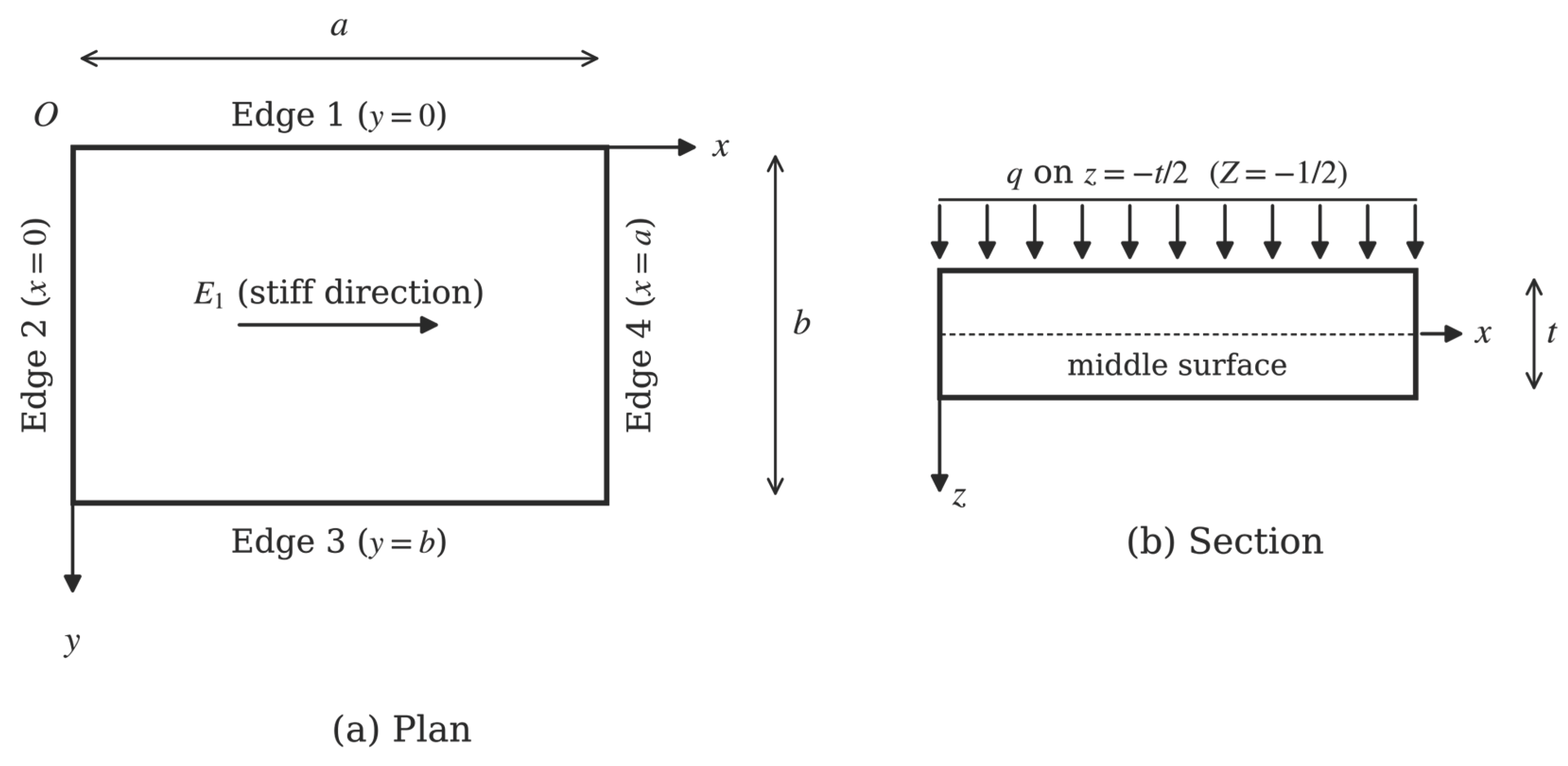
Figure 2.
Deflection along the line through the free-edge midpoint, normal to the free edge (E1/E2 = 25, ∝ = 10): (a) SSFS, β = 1.0; (b) CCFC, β = 1.0; (c) SFSC, β = 2.0; (d) CFCS, β = 2.0.
Figure 2.
Deflection along the line through the free-edge midpoint, normal to the free edge (E1/E2 = 25, ∝ = 10): (a) SSFS, β = 1.0; (b) CCFC, β = 1.0; (c) SFSC, β = 2.0; (d) CFCS, β = 2.0.
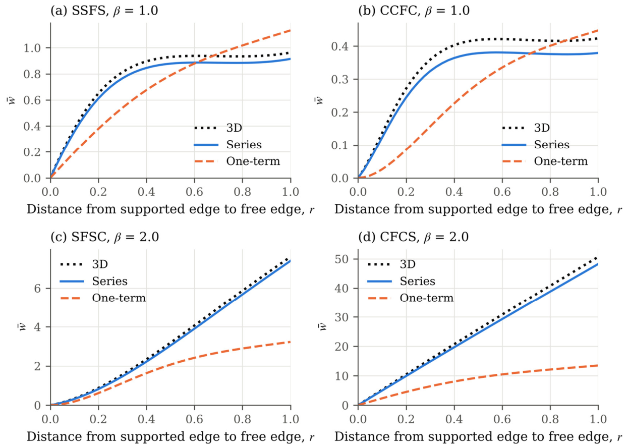
Figure 3.
Deflection of the CCFC plate (E1/E2 = 40, ∝ = 20, β = 1.0): (a) along the line X = 0.5, from clamped edge 1 to the free edge; (b) along the free edge.
Figure 3.
Deflection of the CCFC plate (E1/E2 = 40, ∝ = 20, β = 1.0): (a) along the line X = 0.5, from clamped edge 1 to the free edge; (b) along the free edge.
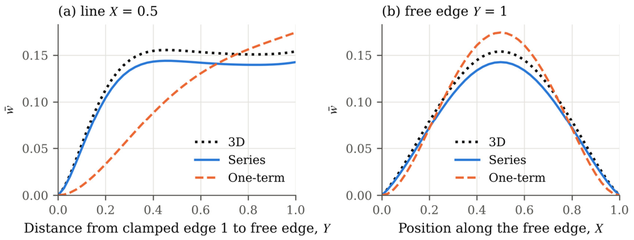
Figure 4.
Ratio of the 3D maximum deflections of plates related by a quarter turn of their supports (free edge across E1 divided by free edge parallel to E1): (a) effect of E1/E2 (∝ = 10, β = 1.0); (b) effect of the aspect ratio (∝ = 10, E1/E2 = 25).
Figure 4.
Ratio of the 3D maximum deflections of plates related by a quarter turn of their supports (free edge across E1 divided by free edge parallel to E1): (a) effect of E1/E2 (∝ = 10, β = 1.0); (b) effect of the aspect ratio (∝ = 10, E1/E2 = 25).
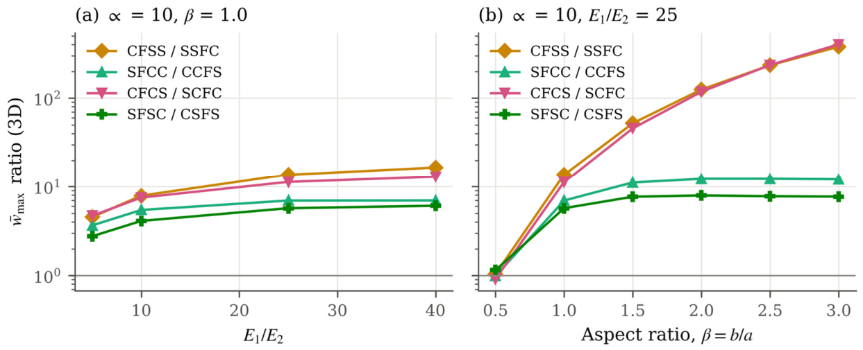
Figure 5.
Theory error of the converged series for the maximum deflection versus the span–thickness ratio (E1/E2 = 25, β = 1.0): (a) free edge parallel to E1; (b) free edge across E1. Plates of the same colour are related by a quarter turn of their supports.
Figure 5.
Theory error of the converged series for the maximum deflection versus the span–thickness ratio (E1/E2 = 25, β = 1.0): (a) free edge parallel to E1; (b) free edge across E1. Plates of the same colour are related by a quarter turn of their supports.
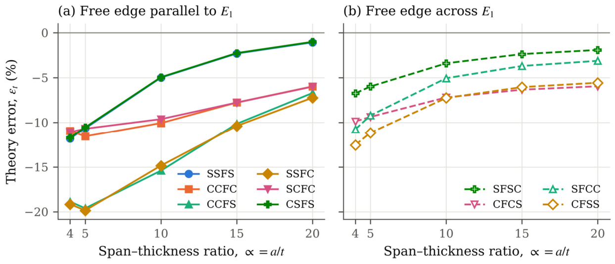
Figure 6.
Theory error of the converged series for the maximum deflection versus the aspect ratio (E1/E2 = 25): (a) ∝ = 4; (b) ∝ = 10.
Figure 6.
Theory error of the converged series for the maximum deflection versus the aspect ratio (E1/E2 = 25): (a) ∝ = 4; (b) ∝ = 10.
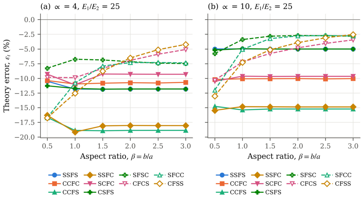
Figure 7.
Theory error with the reduced coefficients versus that with the full coefficients for all 1,200 cases.
Figure 7.
Theory error with the reduced coefficients versus that with the full coefficients for all 1,200 cases.
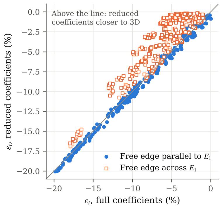
Figure 8.
Total error of the one-term closed form for the maximum deflection versus the aspect ratio (∝ = 10, E1/E2 = 25): (a) free edge parallel to E1; (b) free edge across E1. The shaded band marks ±10%.
Figure 8.
Total error of the one-term closed form for the maximum deflection versus the aspect ratio (∝ = 10, E1/E2 = 25): (a) free edge parallel to E1; (b) free edge across E1. The shaded band marks ±10%.
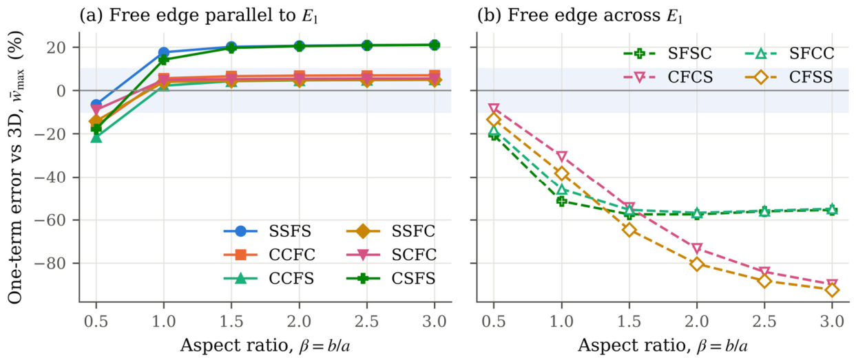
Figure 9.
Number of modular ratios (out of four: E1/E2 = 5, 10, 25, and 40) for which the one-term maximum deflection is within 10% of the 3D value, for each plate, span–thickness ratio, and aspect ratio.
Figure 9.
Number of modular ratios (out of four: E1/E2 = 5, 10, 25, and 40) for which the one-term maximum deflection is within 10% of the 3D value, for each plate, span–thickness ratio, and aspect ratio.
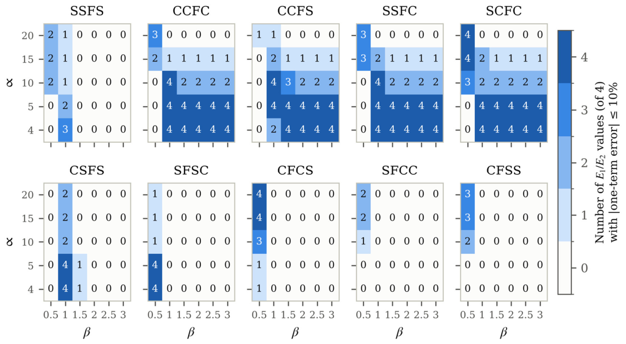
Figure 10.
Error in the normal moment at the clamped mid-edges relative to 3D elasticity, for all clamped edges of the study, grouped by the type of the opposite edge: (a) converged series; (b) one-term solution.
Figure 10.
Error in the normal moment at the clamped mid-edges relative to 3D elasticity, for all clamped edges of the study, grouped by the type of the opposite edge: (a) converged series; (b) one-term solution.
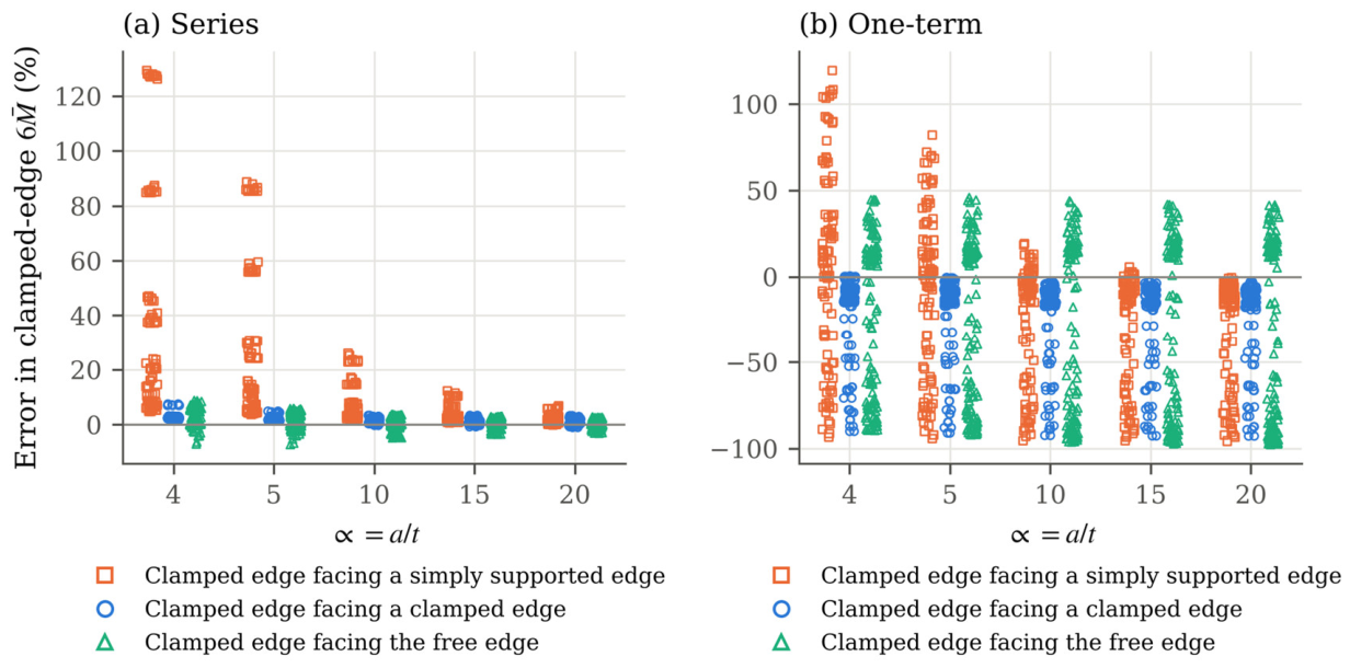
Figure 11.
Through-thickness stress distributions of the CCFC plate (E1/E2 = 25, ∝ = 4, β = 1.0): (a) in-plane normal stress at the free-edge midpoint; (b) transverse shear stress at (X, Y) = (0.25, 0.75); (c) transverse normal stress at (0.5, 0.75).
Figure 11.
Through-thickness stress distributions of the CCFC plate (E1/E2 = 25, ∝ = 4, β = 1.0): (a) in-plane normal stress at the free-edge midpoint; (b) transverse shear stress at (X, Y) = (0.25, 0.75); (c) transverse normal stress at (0.5, 0.75).
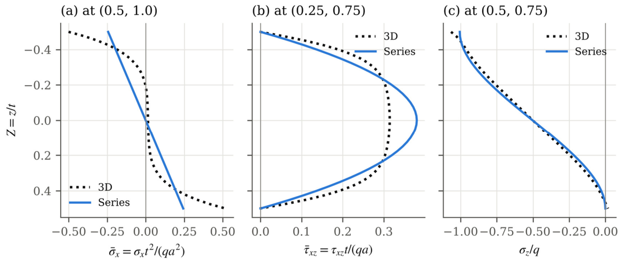

Table 1.
Dimensionless elastic coefficients of the Pagano-type materials (E0 = E2).
| Coefficient | E1/E2 = 5 | E1/E2 = 10 | E1/E2 = 25 | E1/E2 = 40 |
|---|---|---|---|---|
| Δ | 0.906250 | 0.921875 | 0.931250 | 0.933594 |
| c11 | 4.687500 | 9.375000 | 23.437500 | 37.500000 |
| c22 = c33 | 0.987500 | 0.993750 | 0.997500 | 0.998438 |
| c12 = c13 | 0.312500 | 0.312500 | 0.312500 | 0.312500 |
| c23 | 0.262500 | 0.256250 | 0.252500 | 0.251563 |
| c44 | 0.181250 | 0.184375 | 0.186250 | 0.186719 |
| c55 = c66 | 0.453125 | 0.460938 | 0.465625 | 0.466797 |
| (reduced) | 4.588608 | 9.276730 | 23.339599 | 37.402191 |
| (reduced) | 0.917722 | 0.927673 | 0.933584 | 0.935055 |
| (reduced) | 0.229430 | 0.231918 | 0.233396 | 0.233764 |
Table 2.
Edge functions, free-edge orientation, symmetry, and one-term evaluation points of the ten plates.
Table 2.
Edge functions, free-edge orientation, symmetry, and one-term evaluation points of the ten plates.
| Plate | Free edge | Free edge relative to E1 | gx(X) | gy(Y) | Even degrees only in | (X0, Y0) |
|---|---|---|---|---|---|---|
| SSFS | 3 (y = b) | parallel | gSS | gSF | X | (0.5, 1) |
| CCFC | 3 | parallel | gCC | gCF | X | (0.5, 1) |
| CCFS | 3 | parallel | gCS | gCF | – | (0.5785, 1) |
| SSFC | 3 | parallel | gSC | gSF | – | (0.4215, 1) |
| SCFC | 3 | parallel | gCC | gSF | X | (0.5, 1) |
| CSFS | 3 | parallel | gSS | gCF | X | (0.5, 1) |
| SFSC | 2 (x = 0) | perpendicular | gFC | gSS | Y | (0, 0.5) |
| CFCS | 2 | perpendicular | gFS | gCC | Y | (0, 0.5) |
| SFCC | 2 | perpendicular | gFC | gSC | – | (0, 0.4215) |
| CFSS | 2 | perpendicular | gFS | gCS | – | (0, 0.5785) |
Note: (X0, Y0) is the point at which h1 is greatest; the values 0.4215 and 0.5785 are roots of dgSC/dX = 0 and dgCS/dX = 0, respectively.
Table 3.
Constants of the one-term closed-form solution.
| Plate | λ1 | λ2 | λ3 | λ4 | λ5 | λ6 | λ7 |
|---|---|---|---|---|---|---|---|
| SSFS | 146468/37587 | 10462/2211 | 620/3417 | 62/51 | 1715/4556 | 1500/7 | 39/67 |
| CCFC | 124488/8195 | 35568/8195 | 858/745 | 1 | 17493/2980 | 75/7 | 86/149 |
| CCFS | 62244/8195 | 35568/8195 | 2717/2235 | 19/18 | 17493/5960 | 22.2835 | 86/149 |
| SSFC | 36617/4422 | 10462/2211 | 95/603 | 19/18 | 1715/2144 | 89.1339 | 39/67 |
| SCFC | 36617/2211 | 10462/2211 | 10/67 | 1 | 1715/1072 | 300/7 | 39/67 |
| CSFS | 497952/139315 | 35568/8195 | 17732/12665 | 62/51 | 1029/745 | 375/7 | 86/149 |
| SFSC | 17732/12665 | 62/51 | 497952/139315 | 35568/8195 | 1029/745 | 375/7 | 86/149 |
| CFCS | 10/67 | 1 | 36617/2211 | 10462/2211 | 1715/1072 | 300/7 | 39/67 |
| SFCC | 2717/2235 | 19/18 | 62244/8195 | 35568/8195 | 17493/5960 | 22.2835 | 86/149 |
| CFSS | 95/603 | 19/18 | 36617/4422 | 10462/2211 | 1715/2144 | 89.1339 | 39/67 |
Note: λ6 is exact where given as a fraction; for CCFS, SSFC, SFCC, and CFSS, it is given to four decimal places because X0 or Y0 is irrational.
Table 4.
Convergence of the multi-term series with the highest Legendre degree in each direction (full coefficients).
Table 4.
Convergence of the multi-term series with the highest Legendre degree in each direction (full coefficients).
| Case | Highest degree | K | at free-edge midpoint | at free-edge midpoint | G | |
|---|---|---|---|---|---|---|
| (a) SSFS; 25; 4; 1.0 | one-term | 1 | 2.8546 | 2.8546 | 0.9427 | 1.102 |
| 7 | 32 | 2.3121 | 2.3121 | 0.7558 | 0.994 | |
| 15 | 128 | 2.3122 | 2.3122 | 0.7558 | 1.000 | |
| 23 | 288 | 2.3122 | 2.3122 | 0.7558 | 1.000 | |
| 31 | 512 | 2.3122 | 2.3122 | 0.7558 | 1.000 | |
| 39 | 800 | 2.3122 | 2.3122 | 0.7558 | 1.000 | |
| (b) CCFC; 40; 4; 1.0 | one-term | 1 | 1.8485 | 1.8485 | 0.3155 | 1.129 |
| 7 | 32 | 1.6200 | 1.6184 | 0.2431 | 1.005 | |
| 15 | 128 | 1.6692 | 1.6691 | 0.2435 | 0.994 | |
| 23 | 288 | 1.6810 | 1.6810 | 0.2435 | 0.994 | |
| 31 | 512 | 1.6854 | 1.6854 | 0.2435 | 1.003 | |
| 39 | 800 | 1.6876 | 1.6876 | 0.2435 | 0.995 | |
| (c) SFSC; 25; 10; 2.0 | one-term | 1 | 3.2270 | 3.2270 | 0.0406 | 0.160 |
| 7 | 32 | 7.3791 | 7.3791 | 0.0305 | 1.085 | |
| 15 | 128 | 7.3945 | 7.3945 | 0.0305 | 1.000 | |
| 23 | 288 | 7.3983 | 7.3983 | 0.0305 | 0.999 | |
| 31 | 512 | 7.3997 | 7.3997 | 0.0305 | 1.001 | |
| 39 | 800 | 7.4004 | 7.4004 | 0.0305 | 1.000 | |
| (d) CFSS; 40; 20; 3.0 | one-term | 1 | 10.9526 | 10.5324 | 0.0747 | −2.525 |
| 7 | 64 | 219.4969 | 216.0093 | 1.3331 | −0.298 | |
| 15 | 256 | 219.7997 | 216.3116 | 1.3330 | 1.095 | |
| 23 | 576 | 219.8113 | 216.3258 | 1.3332 | 1.034 | |
| 31 | 1024 | 219.8148 | 216.3308 | 1.3334 | 1.020 | |
| 39 | 1600 | 219.8161 | 216.3331 | 1.3335 | 1.011 |
Note: Case gives the plate, E1/E2, ∝, and β. K is the number of terms; only even degrees are used in a direction of symmetry. G is evaluated at (X, Y) = (0.5, 0.75) for SSFS and CCFC and at (0.25, 0.5) for SFSC and CFSS.
Table 5.
Largest residuals of the free-edge conditions over the central 80% of the edge and largest truncation change of the series, over all 120 cases of each plate.
Table 5.
Largest residuals of the free-edge conditions over the central 80% of the edge and largest truncation change of the series, over all 120 cases of each plate.
| Plate | One-term: moment residual (%) | One-term: shear residual (%) | Series: moment residual (%) | Series: shear residual (%) | Series: largest change in with eight more degrees (%) |
|---|---|---|---|---|---|
| SSFS | 100.0 | 46.8 | 0.17 | 2.60 | 0.00 |
| CCFC | 50.0 | 30.3 | 0.64 | 1.01 | 0.25 |
| CCFS | 56.3 | 33.5 | 0.76 | 0.93 | 0.15 |
| SSFC | 56.3 | 31.1 | 3.80 | 1.29 | 0.14 |
| SCFC | 50.0 | 28.0 | 1.79 | 0.94 | 0.14 |
| CSFS | 100.0 | 46.0 | 0.06 | 1.56 | 0.02 |
| SFSC | 18.6 | 11.3 | 0.00 | 1.31 | 0.08 |
| CFCS | 50.0 | 26.9 | 2.15 | 0.90 | 0.12 |
| SFCC | 23.7 | 14.7 | 0.65 | 1.76 | 0.06 |
| CFSS | 56.3 | 28.4 | 1.98 | 0.88 | 0.05 |
Table 6.
Convergence of the 3D Ritz reference and comparison with finite element (FE) solutions.
| Case | Solution | Polynomials or elements (x × y × z) | Unknowns | at free-edge midpoint | at free-edge midpoint | at clamped mid-edge | |
|---|---|---|---|---|---|---|---|
| (a) CCFC; 40; 4; 1.0; edge 2 | 3D Ritz | 10 × 10 × 5 | 1,500 | 1.8346 | 1.8346 | 0.2422 | −0.4673 |
| 3D Ritz | 14 × 14 × 6 | 3,528 | 1.8677 | 1.8677 | 0.2434 | −0.4657 | |
| 3D Ritz | 14 × 14 × 8 | 4,704 | 1.8724 | 1.8724 | 0.2435 | −0.4656 | |
| 3D Ritz | 14 × 14 × 10 | 5,880 | 1.8732 | 1.8732 | 0.2436 | −0.4655 | |
| 3D Ritz | 18 × 18 × 10 | 9,720 | 1.8732 | 1.8732 | 0.2438 | −0.4651 | |
| FE | 24 × 24 × 6 | – | 1.8731 | 1.8731 | 0.2484 | −0.4638 | |
| FE | 32 × 32 × 8 | – | 1.8736 | 1.8736 | 0.2467 | −0.4640 | |
| (b) CFCS; 40; 4; 1.0; edge 1 | 3D Ritz | 10 × 10 × 5 | 1,500 | 9.4796 | 9.4796 | 0.2450 | −0.3598 |
| 3D Ritz | 14 × 14 × 6 | 3,528 | 9.5003 | 9.5003 | 0.2452 | −0.3589 | |
| 3D Ritz | 14 × 14 × 8 | 4,704 | 9.5046 | 9.5046 | 0.2453 | −0.3587 | |
| 3D Ritz | 14 × 14 × 10 | 5,880 | 9.5059 | 9.5059 | 0.2454 | −0.3586 | |
| 3D Ritz | 18 × 18 × 10 | 9,720 | 9.5073 | 9.5073 | 0.2454 | −0.3585 | |
| FE | 24 × 24 × 6 | – | 9.4939 | 9.4939 | 0.2472 | −0.3577 | |
| FE | 32 × 32 × 8 | – | 9.5001 | 9.5001 | 0.2464 | −0.3579 | |
| (c) SFCC; 25; 5; 3.0; edge 4 | 3D Ritz | 8 × 18 × 5 | 2,160 | 11.0293 | 10.9435 | 0.0155 | −3.0870 |
| 3D Ritz | 10 × 24 × 6 | 4,320 | 11.0481 | 10.9620 | 0.0149 | −3.0864 | |
| 3D Ritz | 10 × 24 × 8 | 5,760 | 11.0509 | 10.9649 | 0.0149 | −3.0859 | |
| 3D Ritz | 10 × 24 × 10 | 7,200 | 11.0517 | 10.9657 | 0.0150 | −3.0857 | |
| 3D Ritz | 12 × 30 × 10 | 10,800 | 11.0518 | 10.9658 | 0.0152 | −3.0862 | |
| FE | 12 × 36 × 6 | – | 11.0465 | 10.9606 | 0.0136 | −3.0827 | |
| FE | 16 × 48 × 8 | – | 11.0492 | 10.9633 | 0.0140 | −3.0842 |
Note: Case gives the plate, E1/E2, ∝, β, and the clamped edge at whose midpoint the moment is given. The parametric study used 14 × 14 × 10 polynomials for β = 1.0 and 10 × 24 × 10 for β = 3.0. FE denotes the CalculiX model with C3D20R elements (Section 3.3.3).
Table 7.
Validation of the 3D Ritz reference against the exact solution for the SSSS plate (β = 1.0, centre, on the face Z = 1/2).
Table 7.
Validation of the 3D Ritz reference against the exact solution for the SSSS plate (β = 1.0, centre, on the face Z = 1/2).
| E1/E2 | ∝ | exact | Ritz | Diff. (%) | exact | Ritz | Diff. (%) |
|---|---|---|---|---|---|---|---|
| 10 | 4 | 2.9803 | 2.9803 | −0.0004 | 0.7390 | 0.7390 | −0.005 |
| 10 | 10 | 1.6725 | 1.6725 | −0.0005 | 0.6984 | 0.6984 | +0.005 |
| 10 | 20 | 1.4775 | 1.4775 | 0.0000 | 0.6943 | 0.6943 | +0.001 |
| 25 | 4 | 2.3590 | 2.3590 | −0.0004 | 0.9643 | 0.9641 | −0.020 |
| 25 | 10 | 0.9478 | 0.9478 | −0.0008 | 0.8213 | 0.8214 | +0.006 |
| 25 | 20 | 0.7255 | 0.7255 | 0.0000 | 0.7958 | 0.7958 | +0.002 |
Table 8.
Lévy-type 3D solution versus 3D Ritz reference at the free-edge midpoint (E1/E2 = 25).
| Plate | β | ∝ | Lévy-type | Ritz | Diff. (%) | Lévy-type | Ritz | Diff. |
|---|---|---|---|---|---|---|---|---|
| SSFS | 1.0 | 4 | 2.6222 | 2.6221 | −0.001 | 0.7491 | 0.7492 | 0.0000 |
| SSFS | 1.0 | 10 | 0.9627 | 0.9627 | 0.000 | 0.7695 | 0.7695 | 0.0000 |
| SSFS | 1.0 | 20 | 0.7259 | 0.7259 | −0.001 | 0.7711 | 0.7712 | 0.0000 |
| SSFS | 3.0 | 4 | 2.5438 | 2.5438 | −0.002 | 0.7395 | 0.7400 | +0.0005 |
| SSFS | 3.0 | 10 | 0.9580 | 0.9580 | −0.002 | 0.7631 | 0.7633 | +0.0002 |
| SSFS | 3.0 | 20 | 0.7255 | 0.7255 | +0.001 | 0.7693 | 0.7693 | 0.0000 |
| CSFS | 1.0 | 4 | 2.6219 | 2.6218 | −0.005 | 0.7409 | 0.7408 | −0.0001 |
| CSFS | 1.0 | 10 | 0.9729 | 0.9729 | −0.001 | 0.7751 | 0.7748 | −0.0003 |
| CSFS | 1.0 | 20 | 0.7326 | 0.7326 | +0.002 | 0.7776 | 0.7772 | −0.0004 |
| CSFS | 3.0 | 4 | 2.5440 | 2.5437 | −0.009 | 0.7394 | 0.7399 | +0.0005 |
| CSFS | 3.0 | 10 | 0.9580 | 0.9580 | −0.002 | 0.7627 | 0.7630 | +0.0002 |
| CSFS | 3.0 | 20 | 0.7255 | 0.7255 | 0.000 | 0.7688 | 0.7689 | +0.0001 |
| SFSC | 1.0 | 4 | 9.1714 | 9.1723 | +0.010 | 0.2919 | 0.2921 | +0.0002 |
| SFSC | 1.0 | 10 | 5.5517 | 5.5517 | 0.000 | 0.2149 | 0.2149 | 0.0000 |
| SFSC | 1.0 | 20 | 4.9122 | 4.9121 | −0.002 | 0.2025 | 0.2024 | −0.0001 |
| SFSC | 3.0 | 4 | 13.6660 | 13.6677 | +0.013 | 0.0194 | 0.0194 | 0.0000 |
| SFSC | 3.0 | 10 | 7.2910 | 7.2907 | −0.003 | −0.0026 | −0.0031 | −0.0005 |
| SFSC | 3.0 | 20 | 6.3701 | 6.3696 | −0.008 | −0.0044 | −0.0052 | −0.0007 |
Note: the moment difference is given as an absolute value because the moment parallel to the free edge of the SFSC plate is close to zero in long plates.
Table 9.
Free-edge midpoint values in the thin-plate limit: exact Lévy solution of CPT versus the series and the one-term solution of Alternative 1 Theory at ∝ = 10,000 (full coefficients).
Table 9.
Free-edge midpoint values in the thin-plate limit: exact Lévy solution of CPT versus the series and the one-term solution of Alternative 1 Theory at ∝ = 10,000 (full coefficients).
| Plate | E1/E2 | β | exact (Lévy, CPT) | series | one-term | exact | series |
|---|---|---|---|---|---|---|---|
| SSFS | 10 | 0.5 | 1.7111 | 1.7111 | 1.5412 | 0.8274 | 0.8274 |
| SSFS | 10 | 1.0 | 1.6789 | 1.6789 | 1.9106 | 0.8114 | 0.8114 |
| SSFS | 10 | 2.0 | 1.6449 | 1.6449 | 2.0046 | 0.7945 | 0.7945 |
| SSFS | 10 | 3.0 | 1.6453 | 1.6453 | 2.0218 | 0.7947 | 0.7947 |
| SSFS | 40 | 0.5 | 0.4502 | 0.4502 | 0.4768 | 0.8682 | 0.8682 |
| SSFS | 40 | 1.0 | 0.4035 | 0.4035 | 0.5070 | 0.7759 | 0.7759 |
| SSFS | 40 | 2.0 | 0.4050 | 0.4050 | 0.5133 | 0.7789 | 0.7789 |
| SSFS | 40 | 3.0 | 0.4050 | 0.4050 | 0.5145 | 0.7789 | 0.7789 |
| CSFS | 10 | 0.5 | 1.4400 | 1.4400 | 1.0561 | 0.6927 | 0.6927 |
| CSFS | 10 | 1.0 | 1.6962 | 1.6962 | 1.8384 | 0.8200 | 0.8200 |
| CSFS | 10 | 2.0 | 1.6448 | 1.6448 | 1.9976 | 0.7945 | 0.7945 |
| CSFS | 10 | 3.0 | 1.6453 | 1.6453 | 2.0199 | 0.7947 | 0.7947 |
| CSFS | 40 | 0.5 | 0.4522 | 0.4522 | 0.4179 | 0.8721 | 0.8721 |
| CSFS | 40 | 1.0 | 0.4049 | 0.4049 | 0.5018 | 0.7786 | 0.7786 |
| CSFS | 40 | 2.0 | 0.4050 | 0.4050 | 0.5129 | 0.7789 | 0.7789 |
| CSFS | 40 | 3.0 | 0.4050 | 0.4050 | 0.5144 | 0.7789 | 0.7789 |
| SFSC | 10 | 0.5 | 0.9817 | 0.9817 | 0.8659 | 0.2011 | 0.2011 |
| SFSC | 10 | 1.0 | 7.2825 | 7.2826 | 3.6125 | 0.3601 | 0.3601 |
| SFSC | 10 | 2.0 | 14.4925 | 14.4925 | 4.9078 | 0.1177 | 0.1177 |
| SFSC | 10 | 3.0 | 15.1260 | 15.1260 | 5.0850 | 0.0116 | 0.0116 |
| SFSC | 40 | 0.5 | 0.8966 | 0.8966 | 0.5829 | 0.1833 | 0.1833 |
| SFSC | 40 | 1.0 | 3.3530 | 3.3530 | 1.1849 | 0.1517 | 0.1517 |
| SFSC | 40 | 2.0 | 3.9328 | 3.9328 | 1.2965 | 0.0046 | 0.0046 |
| SFSC | 40 | 3.0 | 3.7504 | 3.7504 | 1.3085 | −0.0039 | −0.0039 |
Table 10.
Benchmark maximum deflections and their location for E1/E2 = 25 and β = 1.0 (full coefficients for the series and one-term solutions).
Table 10.
Benchmark maximum deflections and their location for E1/E2 = 25 and β = 1.0 (full coefficients for the series and one-term solutions).
| Plate | ∝ | , 3D | X | Y | , series | , one-term |
|---|---|---|---|---|---|---|
| SSFS | 4 | 2.6221 | 0.50 | 1.00 | 2.3122 | 2.8546 |
| 10 | 0.9627 | 0.50 | 1.00 | 0.9145 | 1.1329 | |
| 20 | 0.7259 | 0.50 | 1.00 | 0.7180 | 0.8844 | |
| CCFC | 4 | 1.9528 | 0.50 | 1.00 | 1.7389 | 1.9040 |
| 10 | 0.4235 | 0.50 | 1.00 | 0.3808 | 0.4475 | |
| 20 | 0.2033 | 0.50 | 0.49 | 0.1911 | 0.2344 | |
| CCFS | 4 | 2.3259 | 0.51 | 1.00 | 1.8868 | 2.1299 |
| 10 | 0.6147 | 0.54 | 1.00 | 0.5199 | 0.6282 | |
| 20 | 0.3543 | 0.56 | 1.00 | 0.3305 | 0.4091 | |
| SSFC | 4 | 2.3240 | 0.49 | 1.00 | 1.8787 | 2.1751 |
| 10 | 0.6107 | 0.46 | 1.00 | 0.5200 | 0.6349 | |
| 20 | 0.3558 | 0.44 | 0.46 | 0.3300 | 0.4123 | |
| SCFC | 4 | 1.9486 | 0.50 | 1.00 | 1.7324 | 1.9397 |
| 10 | 0.4297 | 0.50 | 0.45 | 0.3884 | 0.4507 | |
| 20 | 0.2068 | 0.50 | 0.38 | 0.1944 | 0.2354 | |
| CSFS | 4 | 2.6218 | 0.50 | 1.00 | 2.3145 | 2.7757 |
| 10 | 0.9729 | 0.50 | 1.00 | 0.9246 | 1.1112 | |
| 20 | 0.7326 | 0.50 | 1.00 | 0.7251 | 0.8694 | |
| SFSC | 4 | 9.1723 | 0.00 | 0.50 | 8.5531 | 6.6278 |
| 10 | 5.5517 | 0.00 | 0.50 | 5.3624 | 2.6952 | |
| 20 | 4.9121 | 0.00 | 0.50 | 4.8175 | 2.0203 | |
| CFCS | 4 | 9.4614 | 0.00 | 0.50 | 8.5263 | 5.9883 |
| 10 | 4.8525 | 0.00 | 0.50 | 4.5025 | 3.3810 | |
| 20 | 4.1479 | 0.00 | 0.50 | 3.9004 | 2.9987 | |
| SFCC | 4 | 7.3818 | 0.00 | 0.46 | 6.5866 | 5.3861 |
| 10 | 4.2776 | 0.00 | 0.44 | 4.0608 | 2.3186 | |
| 20 | 3.7762 | 0.00 | 0.43 | 3.6579 | 1.7818 | |
| CFSS | 4 | 13.1052 | 0.00 | 0.54 | 11.4629 | 7.7090 |
| 10 | 8.3696 | 0.00 | 0.57 | 7.7615 | 5.1672 | |
| 20 | 7.6274 | 0.00 | 0.57 | 7.2021 | 4.8040 |
Table 11.
Benchmark moments for E1/E2 = 25 and β = 1.0: moment parallel to the free edge at its midpoint, and normal moment at the midpoint of the clamped edge with the largest 3D moment.
Table 11.
Benchmark moments for E1/E2 = 25 and β = 1.0: moment parallel to the free edge at its midpoint, and normal moment at the midpoint of the clamped edge with the largest 3D moment.
| Plate | ∝ | Free edge: 3D | Free edge: series | Free edge: one-term | Clamped edge | Clamped: 3D | Clamped: series | Clamped: one-term |
|---|---|---|---|---|---|---|---|---|
| SSFS | 4 | 0.7492 | 0.7558 | 0.9427 | – | – | – | – |
| 10 | 0.7695 | 0.7714 | 0.9634 | – | – | – | – | |
| 20 | 0.7712 | 0.7769 | 0.9669 | – | – | – | – | |
| CCFC | 4 | 0.2467 | 0.2437 | 0.3147 | 2 and 4 | −0.4633 | −0.4728 | −0.4033 |
| 10 | 0.2525 | 0.2505 | 0.3250 | 2 and 4 | −0.5020 | −0.5049 | −0.4164 | |
| 20 | 0.2532 | 0.2540 | 0.3273 | 2 and 4 | −0.5107 | −0.5118 | −0.4193 | |
| CCFS | 4 | 0.5365 | 0.3693 | 0.4684 | 2 | −0.3794 | −0.7031 | −0.6001 |
| 10 | 0.4298 | 0.3800 | 0.4830 | 2 | −0.6460 | −0.7464 | −0.6189 | |
| 20 | 0.3951 | 0.3834 | 0.4863 | 2 | −0.7315 | −0.7594 | −0.6230 | |
| SSFC | 4 | 0.5422 | 0.3733 | 0.4773 | 4 | −0.3967 | −0.7380 | −0.6638 |
| 10 | 0.4278 | 0.3780 | 0.4883 | 4 | −0.6703 | −0.7719 | −0.6790 | |
| 20 | 0.3948 | 0.3826 | 0.4901 | 4 | −0.7443 | −0.7720 | −0.6816 | |
| SCFC | 4 | 0.2498 | 0.2467 | 0.3199 | 2 and 4 | −0.4827 | −0.4954 | −0.4449 |
| 10 | 0.2519 | 0.2497 | 0.3274 | 2 and 4 | −0.5138 | −0.5166 | −0.4553 | |
| 20 | 0.2537 | 0.2541 | 0.3287 | 2 and 4 | −0.5117 | −0.5127 | −0.4571 | |
| CSFS | 4 | 0.7408 | 0.7480 | 0.9184 | 1 | −0.1479 | −0.1548 | −0.1307 |
| 10 | 0.7748 | 0.7776 | 0.9447 | 1 | −0.1459 | −0.1495 | −0.0754 | |
| 20 | 0.7772 | 0.7842 | 0.9504 | 1 | −0.1490 | −0.1525 | −0.0635 | |
| SFSC | 4 | 0.2921 | 0.2862 | 0.2572 | 4 | −2.0148 | −2.0461 | −2.3634 |
| 10 | 0.2149 | 0.2223 | 0.1313 | 4 | −2.4632 | −2.4597 | −2.9579 | |
| 20 | 0.2024 | 0.2137 | 0.1024 | 4 | −2.5509 | −2.5333 | −3.0944 | |
| CFCS | 4 | 0.2448 | 0.2456 | 0.2261 | 1 and 3 | −0.3597 | −0.3688 | −0.3144 |
| 10 | 0.2826 | 0.2870 | 0.2413 | 1 and 3 | −0.3685 | −0.3725 | −0.3355 | |
| 20 | 0.2960 | 0.3001 | 0.2447 | 1 and 3 | −0.3695 | −0.3730 | −0.3403 | |
| SFCC | 4 | 0.2220 | 0.2061 | 0.2032 | 4 | −1.6323 | −1.5826 | −1.8511 |
| 10 | 0.1919 | 0.1968 | 0.1297 | 4 | −1.9232 | −1.8912 | −2.4423 | |
| 20 | 0.1911 | 0.1991 | 0.1073 | 4 | −2.0088 | −1.9743 | −2.6227 | |
| CFSS | 4 | 0.3575 | 0.3425 | 0.2859 | 1 | −0.4499 | −0.5123 | −0.3976 |
| 10 | 0.3936 | 0.3968 | 0.2886 | 1 | −0.4968 | −0.5086 | −0.4014 | |
| 20 | 0.4090 | 0.4144 | 0.2892 | 1 | −0.5043 | −0.5065 | −0.4022 |
Note: where two clamped edges are listed, they carry the same moment by symmetry.
Table 12.
Ranges of the theory error and the total one-term error for the maximum deflection (%), over the four modular ratios and six aspect ratios, and number of cases in which the one-term error is within ±10%.
Table 12.
Ranges of the theory error and the total one-term error for the maximum deflection (%), over the four modular ratios and six aspect ratios, and number of cases in which the one-term error is within ±10%.
| Plate | εt full, ∝ = 4 | εt full, ∝ = 20 | εt reduced, ∝ = 4 | εt reduced, ∝ = 20 | One-term total, ∝ = 4 | One-term total, ∝ = 20 | Cases within ±10% (of 120) |
|---|---|---|---|---|---|---|---|
| SSFS | −12.5 to −5.8 | −2.2 to 0.0 | −13.1 to −5.8 | −3.0 to −0.4 | −18.2 to 16.2 | −17.6 to 24.9 | 14 |
| CCFC | −12.0 to −9.5 | −7.4 to −2.1 | −12.3 to −9.2 | −8.2 to −1.8 | −22.8 to 4.5 | −17.1 to 20.2 | 62 |
| CCFS | −19.3 to −14.5 | −9.6 to −1.9 | −19.7 to −14.1 | −10.3 to −1.8 | −26.1 to −0.2 | −25.6 to 20.2 | 59 |
| SSFC | −19.4 to −14.1 | −9.7 to −1.8 | −19.9 to −14.2 | −10.6 to −1.8 | −25.2 to −0.1 | −11.2 to 20.3 | 64 |
| SCFC | −12.0 to −8.0 | −7.5 to −2.1 | −12.5 to −8.0 | −8.2 to −1.8 | −22.2 to 4.5 | −4.9 to 20.2 | 67 |
| CSFS | −12.5 to −5.8 | −2.2 to 0.0 | −12.9 to −6.3 | −2.9 to −0.4 | −22.6 to 16.1 | −35.3 to 24.9 | 16 |
| SFSC | −8.4 to −4.4 | −5.1 to −0.9 | −8.5 to −3.4 | −1.2 to −0.2 | −54.8 to −3.7 | −66.0 to −9.2 | 11 |
| CFCS | −11.0 to −5.1 | −8.0 to −3.0 | −10.4 to −2.9 | −3.0 to −0.2 | −91.2 to −8.2 | −93.4 to 8.2 | 13 |
| SFCC | −17.7 to −4.7 | −7.9 to −0.9 | −16.7 to −3.4 | −3.2 to −0.2 | −53.9 to −14.1 | −65.2 to −2.8 | 5 |
| CFSS | −17.9 to −4.2 | −8.4 to −2.1 | −16.9 to −2.6 | −3.3 to −0.2 | −93.0 to −13.9 | −95.1 to 2.3 | 8 |
Disclaimer/Publisher’s Note: The statements, opinions and data contained in all publications are solely those of the individual author(s) and contributor(s) and not of MDPI and/or the editor(s). MDPI and/or the editor(s) disclaim responsibility for any injury to people or property resulting from any ideas, methods, instructions or products referred to in the content. |
© 2026 by the authors. Licensee MDPI, Basel, Switzerland. This article is an open access article distributed under the terms and conditions of the Creative Commons Attribution (CC BY) license (http://creativecommons.org/licenses/by/4.0/).
Copyright: This open access article is published under a Creative Commons CC BY 4.0 license, which permit the free download, distribution, and reuse, provided that the author and preprint are cited in any reuse.