Realistic Wind–Wave Loading Versus the Hub-Load Idealisation: Lateral Response of a Large-Diameter Offshore Wind Turbine Monopile

1. Introduction

The increasing demand for clean and sustainable energy has made offshore wind one of the fastest-growing renewable energy sources, with installed capacity expanding over the past two decades across Europe, Asia and North America. As individual turbine ratings have grown from 2–3 MW to beyond 10 MW, foundation systems have had to keep pace. Among the available substructures, monopiles have become by far the most widely adopted, accounting for around 80% of offshore wind installations Europe (Wind Europe, 2021) .

Offshore wind turbines are subjected to a complex combination of lateral environmental loads throughout their service life. Aerodynamic loads arise from the interaction of wind with the rotor, producing a thrust force at hub height, together with distributed wind drag along the tower (Arany et al., 2017; Deng et al., 2025; Jonkman et al., 2009). Hydrodynamic loads result from wave and current action on the submerged part of the monopile and are usually computed with Morison's equation, which accounts for both inertia and drag (Det Norske Veritas, 2007; Morison et al., 1950) . Together these loads generate large lateral forces and overturning moments at the mudline, which must be transferred safely to the surrounding soil by the embedded part of the monopile. Several studies have shown that the wind load at the hub has the greatest influence on the structural response under operating conditions, whereas wave loads become increasingly dominant in extreme sea states (Arany et al., 2017; Jawalageri et al., 2024; Shi et al., 2012). Accurate characterisation of these loads, and of how they are transferred to the soil, is therefore fundamental to safe and economical monopile design.

The literature on laterally loaded monopiles includes extensive experimental, analytical and numerical work. The early field tests of Reese et al. (1974) and Matlock (1970) on small-diameter piles established the basis of the p–y method. Centrifuge programmes later extended this understanding to large-diameter monopiles. Choo et al. (2014) and Choo and Kim (2015) developed p–y relationships from centrifuge tests and showed that the API p–y method overestimates the initial stiffness and underestimates the ultimate soil resistance of large-diameter monopiles. Klinkvort and Hededal (2014) examined the effects of load eccentricity and stress level in centrifuge tests, and LeBlanc et al. (2010) performed laboratory tests on stiff piles in sand, both confirming the rigid-body rotation of monopiles with low length-to-diameter ratios under monotonic and cyclic loading. Finite-element (FE) modelling has become an important tool for studying monopile behaviour beyond the limitations of the p–y framework. Lesny and Wiemann (2006) were among the first to use 3D FE models to examine the diameter-dependent lateral response of monopiles, and Achmus et al. (2009) investigated cyclic behaviour with a stiffness-degradation model.

Some of the most relevant recent studies are summarized in Table 1. Ahmed and Hawlader (2016) analysed large-diameter monopiles in dense sand with a modified Mohr–Coulomb model, Murphy et al. (2018) proposed a 3D FE approach for monopile design that includes interface contact modelling, and Khezri et al. (2024) studied the effect of slenderness ratio in clay. Recent studies have also extended large-diameter monopile analysis to partially rock-socketed foundations. Sadiq et al. (2025b) developed and centrifuge-validated a nonlinear 3D FE model for partially rock-socketed monopiles and combined the numerical database with machine-learning models to predict ultimate lateral capacity, while Sadiq et al. (2025a) investigated flexible, semi-rigid, and rigid rock-socketed monopiles to quantify the effects of stiffness and rock socketing on lateral capacity, deformation mode, earth-pressure distribution, bending response, and local p–y behaviour. A major development in large diameter monopile design was the PISA joint industry project, in which field tests at Cowden (stiff glacial clay till) were combined with 3D FE modeling (Burd et al., 2019; Byrne et al., 2017, 2019a) Similarly combined field tests at Dunkirk (dense marine sand) with 3D FE modelling (Taborda et al., 2019; Zdravkovic et al., 2019). The resulting design framework uses four soil-reaction components: distributed lateral load, distributed moment, base shear and base moment. Alternative soil-reaction frameworks have also been proposed, including a CPT-based p–y formulation validated against 3D FE and full-scale tests (Suryasentana and Lehane, 2016). Futher improved p–y approaches for large-diameter piles (Thieken et al., 2015), a unified ‘p–y + M_R–θ_R’ model for soft clay (Wang et al., 2020) , and beam-theory approaches (Gupta and Basu, 2018) . Complementary centrifuge programmes in clay have clarified the soil-flow mechanisms that govern the transition between flexible, semi-rigid and rigid pile behaviour (Hong et al., 2017; Kong et al., 2022; Lai et al., 2020). Studies that focus specifically on the depth-wise earth-pressure distribution around laterally loaded monopiles are comparatively scarce, yet they are important for understanding how resistance is mobilised. Ma and Yang (2023) carried out a comprehensive 3D FE study of how pile diameter influences the earth pressure distribution and soil deformation mechanisms around monopiles. They considered diameters of 2, 5 and 10 m, representing flexible, semi-rigid and rigid behaviour, all embedded 25 m in dense sand modelled with the Mohr–Coulomb criterion(Coulomb et al., 2023; Mohr, 1882) . They found that the normalised earth pressure distribution changes considerably with pile diameter, so theoretical stress distributions derived from small-diameter pile tests cannot be applied directly to large-diameter monopiles. Choo and Kim (2015) provided complementary centrifuge evidence that earth-pressure mobilisation around large-diameter monopiles differs fundamentally from that around conventional small-diameter piles.

Despite these advances, a common limitation persists in continuum-based geotechnical studies of monopiles: soil mobilisation and earth-pressure development are typically investigated using a single eccentric load applied above the mudline. Offshore wind turbines are in fact loaded simultaneously by three spatially distributed actions: the aerodynamic thrust at hub height, the wind drag along the tower, and the hydrodynamic load on the submerged monopile (Jonkman, 2007; Morison et al., 1950) . Wave loads act directly on the monopile between the seabed and the sea surface and change the bending-moment distribution along the submerged pile (Shi et al., 2012) Moreover, the relative contribution of the three components varies with environmental conditions: during extreme sea states the wave load increases sharply while the rotor thrust is reduced by pitching or parking the rotor (Det Norske Veritas, 2007; IEC 61400-3-1, 2019) . Consequently, the ratio of mudline moment to horizontal load, and therefore the effective height of the resultant load, varies substantially between loading scenarios. Classical rigid-pile theory shows that this effective height controls the position of the rotation point and the distribution of soil resistance (Guo, 2008; Zhang et al., 2005) . However, the effect of realistic distributed wind–wave loading on monopile deformation, bending response, earth-pressure redistribution, and local soil mobilisation has, to the authors’ knowledge not yet been examined systematically.

The present study addresses the gap associated with the conventional point-load assumption by considering the spatial distribution of wind and wave loading along the offshore wind-turbine system. A three-dimensional coupled FE model of the NREL 5 MW reference turbine (Jonkman et al., 2009) including the monopile and surrounding dense sand, is developed in Abaqus (Dassault Systèmes, 2017) and validated in two stages. The same three loading scenarios are analysed using both the three-dimensional continuum FE model and the nonlinear p–y spring model: (i) a single concentrated load at hub height, the conventional idealisation; (ii) rated wind combined with a normal sea state (NSS); and (iii) extreme wind combined with an extreme sea state (ESS), defined following (IEC 61400-3-1, 2019). Pile geometry, soil properties, model parameters, and the serviceability limit state (SLS) and ultimate limit state (ULS) definitions are kept identical across the three loading scenarios within each modelling approach, so that the observed differences can be attributed to the load distribution, that is, to the resulting force–moment combination.

The central objective is to determine how the realistic spatial distribution of wind and wave loading alters the lateral force–moment demand, rotation, deformation pattern, bending response and depth-wise mobilisation of soil resistance relative to the conventional single-hub-load idealisation, and to identify which of these effects are independent of the modelling approach. The novelty of the study lies in quantifying these effects in a coupled turbine–monopile–soil framework, using both continuum and p–y representations. Three research questions are addressed: (i) at the same mudline displacement, how does realistic load distribution change the lateral load, overturning moment and rotation relative to the single-hub-load idealisation; (ii) how does it change the deformation mechanism, the bending-moment distribution, the pile–soil contact pressure (continuum model) and the net soil-reaction mobilisation; and (iii) which of these effects appear in both the continuum and p–y models. Section 2 describes the model development, validation procedure, load cases, SLS and ULS assessment criteria, and analysis methodology. Section 3 presents and discusses the results, Section 4 and Section 5 summarise the engineering implications and the study limitations, respectively, and Section 6 presents the conclusions.

Table 1. Summary of the most relevant recent studies on laterally loaded offshore monopiles.

Reference	Approach	Soil type	Pile (D; L/D)	Loading type	Primary focus / key finding
(Ahmed and Hawlader, 2016)	3D FE	Dense sand	Large D; varied	Single eccentric load	Modified Mohr–Coulomb model for static lateral capacity of large-diameter monopiles
(Byrne et al., 2019a)	Field + 3D FE	Sand & clay	0.27–2.0 m; 3–10	Single lateral load + moment	PISA framework with p–y, m–θ, base shear and base moment components
(Wang et al., 2020) )	3D FE + analytical	Soft clay	Flexible–rigid; varied	Single lateral load + moment	Unified ‘p–y + MR–θR’ soil-reaction model reducing design conservatism
(Kong et al., 2022)	Centrifuge	Kaolin clay	Large D; varied	Monotonic + cyclic lateral	Monotonic and cyclic lateral behaviour and soil reaction of monopiles in clay
(Ma and Yang, 2023)	3D FE	Dense sand	2, 5, 10 m; L = 25 m	Single eccentric load	Earth pressure distribution and soil deformation vs diameter (flexible/semi-rigid/rigid)
(Khezri et al., 2024)	3D FE	Clay	Varied; 3–7	Single eccentric load	Effect of slenderness ratio on lateral capacity, deformation and soil reaction
(Sadiq et al., 2025b)	3D FE + ML	Sand over rock	240 configurations; L, D and e varied	Single eccentric load	ML prediction of lateral capacity of partially rock-socketed monopiles; XGBoost most accurate (R² = 0.986); SHAP feature importance D > e > L > Dr
(Sadiq et al., 2025a)	3D FE	Sand over rock	Flexible/semi-rigid/rigid	Single eccentric load	Lateral earth pressure and p–y of rock-socketed monopiles
Present study	Coupled 3D FE + p–y	Dense sand	5 m; 5	Distributed thrust + tower drag + wave	Effect of realistic load distribution on structural response and soil mobilisation

Table 1. Summary of the most relevant recent studies on laterally loaded offshore monopiles.

Reference	Approach	Soil type	Pile (D; L/D)	Loading type	Primary focus / key finding
(Ahmed and Hawlader, 2016)	3D FE	Dense sand	Large D; varied	Single eccentric load	Modified Mohr–Coulomb model for static lateral capacity of large-diameter monopiles
(Byrne et al., 2019a)	Field + 3D FE	Sand & clay	0.27–2.0 m; 3–10	Single lateral load + moment	PISA framework with p–y, m–θ, base shear and base moment components
(Wang et al., 2020) )	3D FE + analytical	Soft clay	Flexible–rigid; varied	Single lateral load + moment	Unified ‘p–y + MR–θR’ soil-reaction model reducing design conservatism
(Kong et al., 2022)	Centrifuge	Kaolin clay	Large D; varied	Monotonic + cyclic lateral	Monotonic and cyclic lateral behaviour and soil reaction of monopiles in clay
(Ma and Yang, 2023)	3D FE	Dense sand	2, 5, 10 m; L = 25 m	Single eccentric load	Earth pressure distribution and soil deformation vs diameter (flexible/semi-rigid/rigid)
(Khezri et al., 2024)	3D FE	Clay	Varied; 3–7	Single eccentric load	Effect of slenderness ratio on lateral capacity, deformation and soil reaction
(Sadiq et al., 2025b)	3D FE + ML	Sand over rock	240 configurations; L, D and e varied	Single eccentric load	ML prediction of lateral capacity of partially rock-socketed monopiles; XGBoost most accurate (R² = 0.986); SHAP feature importance D > e > L > Dr
(Sadiq et al., 2025a)	3D FE	Sand over rock	Flexible/semi-rigid/rigid	Single eccentric load	Lateral earth pressure and p–y of rock-socketed monopiles
Present study	Coupled 3D FE + p–y	Dense sand	5 m; 5	Distributed thrust + tower drag + wave	Effect of realistic load distribution on structural response and soil mobilisation

2. Methodology

The overall methodology is summarised in Figure 1. The modelling framework begins with a two-stage validation procedure in which the turbine superstructure and the pile–soil subsystem are validated separately (Section 2.1). The validated components are then integrated into a three-dimensional coupled turbine–monopile–soil finite-element model in Abaqus/Standard (Section 2.2). Three loading scenarios, a conventional single concentrated load at hub height, rated wind combined with a normal sea state (NSS), and extreme wind combined with an extreme sea state (ESS), are defined in Section 2.3 and applied consistently to both the three-dimensional continuum model and the nonlinear p–y spring model. The p–y model is introduced in Section 2.4 as an independent soil-reaction representation for evaluating whether the observed loading-distribution effects are robust to the adopted soil-pile interaction formulation. Responses from both modelling approaches are then evaluated at common displacement-based serviceability limit state (SLS) and ultimate limit state (ULS) criteria (Section 2.5), enabling systematic comparison of global response, bending demand, deformation mechanisms, earth-pressure and soil-reaction profiles, and local p–y behaviour.

Figure 1. Flowchart of the methodology: model development and two-stage validation, load-case definition, continuum and p–y analyses, and post-processing at SLS and ULS.

Figure 1. Flowchart of the methodology: model development and two-stage validation, load-case definition, continuum and p–y analyses, and post-processing at SLS and ULS.

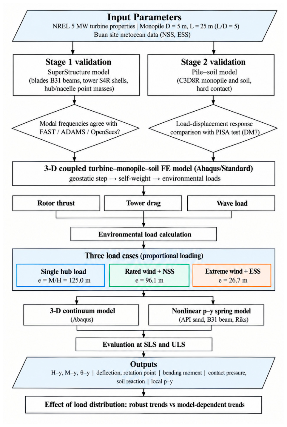
Table 2. Properties of the NREL 5 MW reference wind turbine (Jonkman et al., 2009) .

Component	Property	Value
Rotor	Rated power	5 MW
	Rotor diameter (m)	126
	Hub height (m)	90
	Cut-in; rated; cut-out wind speed (m/s)	3; 11.4; 25
Blade	Length (m)	61.5
	Overall mass (kg)	53,220
Hub–nacelle	Hub mass (kg)	56,780
	Nacelle mass (kg)	240,000
Tower	Height (m)	90
	Base; top outer diameter (m)	6.0; 3.87
	Base; top wall thickness (m)	0.027; 0.0119
	Steel E (GPa); ν; ρ (kg/m³)	210; 0.3; 8500

Table 2. Properties of the NREL 5 MW reference wind turbine (Jonkman et al., 2009) .

Component	Property	Value
Rotor	Rated power	5 MW
	Rotor diameter (m)	126
	Hub height (m)	90
	Cut-in; rated; cut-out wind speed (m/s)	3; 11.4; 25
Blade	Length (m)	61.5
	Overall mass (kg)	53,220
Hub–nacelle	Hub mass (kg)	56,780
	Nacelle mass (kg)	240,000
Tower	Height (m)	90
	Base; top outer diameter (m)	6.0; 3.87
	Base; top wall thickness (m)	0.027; 0.0119
	Steel E (GPa); ν; ρ (kg/m³)	210; 0.3; 8500

2.1. Model Validation

The reliability of the modelling framework was established through a two-stage validation procedure. In the first stage, the superstructure model of the NREL 5 MW reference turbine was validated against published modal frequencies obtained using FAST, ADAMS, and OpenSees (Jonkman and Buhl, 2005; Mazzoni et al., 2006; MSC Software, n.d.) In the second stage, the pile–soil interaction model was validated against the PISA benchmark (Burd et al., 2019; Byrne et al., 2019b) . Validating the structural and geotechnical components separately allows the dynamic response of the tower–rotor–nacelle assembly and the lateral response of the embedded monopile–soil system to be assessed independently before the two components are integrated into the coupled model.

2.1.1. NREL 5 MW Reference Wind Turbine

The NREL 5 MW baseline is a conventional three-bladed, upwind, variable-speed offshore reference turbine (Jonkman et al., 2009) . It has a rated power of 5 MW, a hub height of 90 m, a rotor diameter of 126 m and a rated wind speed of 11.4 m/s, with cut-in and cut-out wind speeds of 3 and 25 m/s. The principal properties adopted in the present model are listed in Table 2.

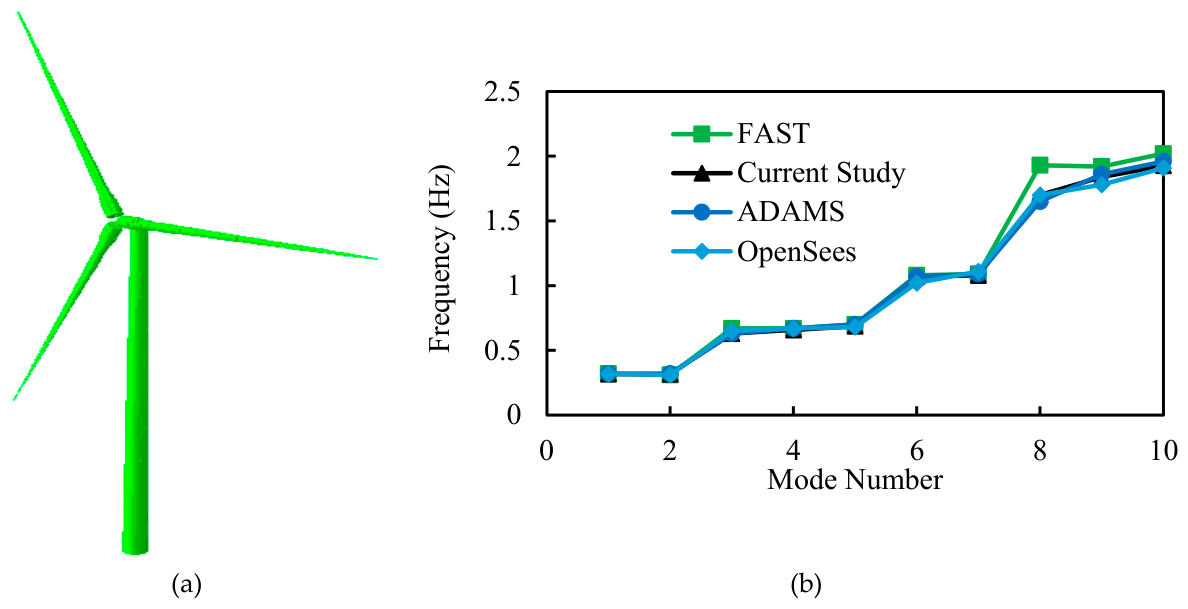
The turbine was modelled in Abaqus based on the NREL 5 MW reference definition (Figure 2a). The three blades were represented by two-node linear beam elements (B31) with the distributed structural properties of the reference blade, and the tapered tower was discretised with four-node reduced- integration shell elements (S4R). The hub and nacelle were idealised as concentrated inertial point masses at their centres of gravity. Distributing coupling constraints connected the tower top to the hub, the hub to the three blade roots, and the hub to the nacelle mass, so that loads and inertia were transferred consistently without artificial local stiffening. An effective tower steel density of 8500 kg/m³ was adopted to account for secondary components such as bolts, flanges, welds and paint that are not modelled explicitly (Jonkman et al., 2009) . For this validation stage, the tower base was fully fixed, so that the computed frequencies represented the dynamic characteristics of the superstructure alone and could therefore be compared directly with the published reference values.

The dynamic characteristics of the assembled superstructure were obtained using a linear perturbation frequency-extraction procedure with the Lanczos eigen solver. The first ten natural frequencies were compared with the FAST, ADAMS, and OpenSees results (Figure 2b). The lower modes are governed by the first fore–aft and side-to-side bending of the tower together with the first flap wise blade modes, while the higher modes correspond to edgewise blade modes and second-order blade and tower bending. The frequencies predicted by the present model agree closely with all three reference codes. They coincide almost exactly with the ADAMS and OpenSees results, and the only appreciable spread occurs in modes 8–10, where the FAST predictions are slightly higher, which is consistent with differences in modelling assumptions and structural idealisation among the reference codes. On this basis, the superstructure model was considered sufficiently validated for integration with the pile–soil subsystem and was retained unchanged in the subsequent coupled analyses.

Figure 2. Validation of superstructure: (a) NREL 5 MW wind turbine ABAQUS Model (b) comparison of the first ten natural frequencies with FAST, ADAMS and OpenSees.

Figure 2. Validation of superstructure: (a) NREL 5 MW wind turbine ABAQUS Model (b) comparison of the first ten natural frequencies with FAST, ADAMS and OpenSees.

2.1.2. Pile–Soil Interaction Model

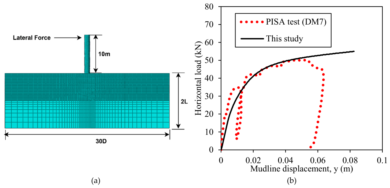
The developed three-dimensional finite-element (FE) model was validated against the well-documented PISA field tests conducted at the Dunkirk site in northern France. The PISA DM7 field test was selected as the benchmark case because its embedded length lies entirely within the upper hydraulically placed sand layer, thereby reducing the influence of the underlying soil stratum on the measured lateral response. The DM7 pile had a diameter of 0.762 m, an embedded length of 2.29 m (L/D =3), and was subjected to lateral loading at a height of 10 m above the ground surface. For consistency with the subsequent analyses, the ultimate limit state (ULS) was taken as a mudline displacement equal to 10% of the pile diameter (0.1D).

The upper soil layer consisted of dense hydraulically placed sand with a relative density of 100% and an initial void ratio of 0.54. During the field test, the groundwater table was located approximately 5.4 m below the ground surface, placing the entire embedded length of the DM7 pile above the recorded groundwater level. The saturated unit weight and at-rest earth-pressure coefficient of the sand were 17.1 kN/m³ and 0.4, respectively.

Figure 3a shows the FE computational domain, while Figure 3b compares the predicted and measured lateral load–mudline displacement responses. The FE model shows close agreement with the field response over the displacement range considered, capturing the initial stiffness and subsequent nonlinear load–displacement behaviour with only minor deviation from the measured curve. This agreement supports the adopted soil constitutive representation and pile–soil contact formulation for modelling the lateral response of monopiles in dense sand.

Figure 3. Validation of the pile–soil interaction model: (a) FE representation of the PISA DM7 benchmark and (b) comparison between measured and predicted lateral load–mudline displacement response.

Figure 3. Validation of the pile–soil interaction model: (a) FE representation of the PISA DM7 benchmark and (b) comparison between measured and predicted lateral load–mudline displacement response.

2.2. Three-Dimensional Coupled Finite-Element Model

The validated superstructure and pile–soil subsystem were combined into a single 3D coupled FE model in Abaqus/Standard (Figure 4). The model reproduces the complete load path of an operating offshore wind turbine, from the aerodynamic and hydrodynamic actions on the structure, through the tower and monopile, into the surrounding soil. Accordingly, the pile–soil interface response develops under the applied spatially distributed loading rather than from a prescribed equivalent point load. The superstructure is modelled using the same discretization and structural properties adopted in the validated configuration described in Section 2.1.1.

The monopile has a diameter of 5 m and is embedded 25 m in the seabed (L/D = 5). It passes through 25 m of water and extends 10 m above the still-water level to the transition piece and tower base. The NREL reference hub is 90 m above the tower base; therefore, the hub is 100 m above still-water level and 125 m above the mudline. The wall thickness, (t=113 mm, was selected following the API recommendation (API, 2014). The monopile is discretized with eight-node reduced-integration solid elements (C3D8R). A solid-element representation was adopted to provide an explicit three-dimensional pile–soil contact surface and to facilitate calculation of interface pressure and soil reaction around the pile circumference.

Figure 4. 3D Three-dimensional coupled turbine–monopile–soil finite-element model and mesh.

Figure 4. 3D Three-dimensional coupled turbine–monopile–soil finite-element model and mesh.

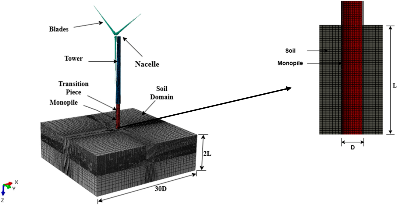
The soil is also discretized using C3D8R elements. The sand is modelled as an elastic–perfectly plastic material obeying the Mohr–Coulomb failure criterion with a non-associated flow rule. The lateral boundaries of the soil domain extend to 30D from the pile, and the domain depth is 2L, following previous numerical studies (Ahmed and Hawlader, 2016; Wang et al., 2020) to minimize boundary influence on the monopile response. The mesh is refined in the pile near field, where earth-pressure and deformation gradients are highest, and gradually coarsened toward the outer boundaries. The base of the soil domain is fully fixed, while the vertical boundaries are restrained in the direction normal to each face.

Pile–soil interaction is modelled using surface-to-surface finite-sliding contact along the outer shaft and pile base. A hard-contact normal pressure–overclosure formulation with separation permitted allows a gap to develop on the active side of the laterally deflecting pile, while tangential behaviour is governed by a penalty-friction formulation with a coefficient of μ = 0.62. The model is initialized through a geostatic step in which the in-situ effective-stress state is generated using the prescribed K₀ condition and the effective unit weight of the submerged sand. Turbine self-weight is subsequently applied, followed by the environmental loading histories. All reported displacements and rotations are referenced to the equilibrium configuration obtained after completion of the geostatic and self-weight steps, thereby isolating the response induced by the applied environmental loading.

The environmental conditions adopted for the normal and extreme loading scenarios are summarized in Table 3. The normal sea state (NSS) represents operation at the rated hub-height wind speed of 11.4 m/s, whereas the extreme sea state (ESS) represents the parked-turbine condition under an extreme hub-height wind speed of 33.83 m/s. The associated wave and current parameters are taken from the Sangwangdeungdo, Buan site conditions reported by Noh and Sun (2025).

Table 3. Environmental conditions adopted for the normal sea state (NSS) and extreme sea state (ESS) at Sangwangdeungdo, Buan (Noh and Sun, 2025) .

Parameter	Symbol	Normal (NSS)	Extreme (ESS)	Unit
Hub wind speed	Vhub	11.4	33.83	m/s
Turbine state	–	Operating	Parked	–
Significant wave height	Hs	1.0	5.41	m
Peak period	Tp	5.5	10.44	s
Surface current	Vc	0.5	1.5	m/s
Water depth	d	25	25	m

Table 3. Environmental conditions adopted for the normal sea state (NSS) and extreme sea state (ESS) at Sangwangdeungdo, Buan (Noh and Sun, 2025) .

Parameter	Symbol	Normal (NSS)	Extreme (ESS)	Unit
Hub wind speed	Vhub	11.4	33.83	m/s
Turbine state	–	Operating	Parked	–
Significant wave height	Hs	1.0	5.41	m
Peak period	Tp	5.5	10.44	s
Surface current	Vc	0.5	1.5	m/s
Water depth	d	25	25	m

2.3. Environmental Loads and Load Cases Definition

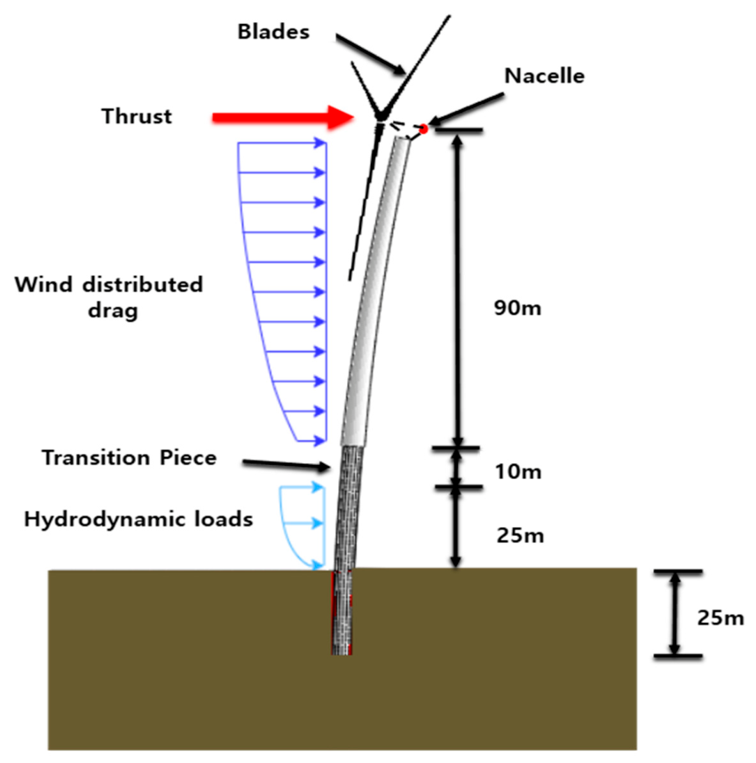
The environmental conditions adopted in this study were derived from the Buan offshore area on the west coast of South Korea, where the relatively shallow water depth is suitable for monopile-supported offshore wind turbines. Figure 5 illustrates the principal environmental actions considered for the NREL 5 MW reference turbine. The loading framework includes aerodynamic thrust at the rotor, distributed wind drag along the tower, and hydrodynamic loading along the submerged monopile.

Three loading scenarios are considered. The first is a conventional single concentrated load applied at hub height, consistent with the idealisation commonly adopted in previous monopile studies, and is used as a reference case. The second represents rated operation under a normal sea state (NSS), combining rotor thrust, tower wind drag, and wave loading. The third represents a parked turbine subjected to an extreme wind condition together with an extreme sea state (ESS). The environmental parameters adopted for the NSS and ESS conditions are summarized in Table 3.

Under the NSS condition, the dominant contribution to the global lateral demand is the rotor thrust acting at hub height, resulting in a relatively large effective loading height above the mudline. Under the ESS condition, rotor thrust is reduced because the turbine is parked, whereas the hydrodynamic load on the submerged monopile increases substantially. Consequently, the dominant lateral action shifts downward toward the mudline. The three loading scenarios therefore differ not only in total horizontal force and overturning moment, but also in the spatial distribution of load along the turbine–monopile system. This distinction forms the basis for evaluating whether an equivalent single-point-load idealisation can reproduce the structural and soil-response mechanisms generated by realistic distributed environmental loading.

Figure 5. Schematic representation of aerodynamic and hydrodynamic loading on the NREL 5 MW offshore wind-turbine system.

Figure 5. Schematic representation of aerodynamic and hydrodynamic loading on the NREL 5 MW offshore wind-turbine system.

2.3.1. Wind Loads

The aerodynamic thrust on the rotor is calculated following (Arany et al., 2017) :

F_Th = 0.5 C_T ρ_a V_hub² A_swept

(1)

where ρ_a is the air density, A_swept the rotor swept area, C_T the thrust coefficient and V_hub the wind speed at hub height.

Between the cut-in and rated wind speeds the thrust coefficient is obtained from the expression (Frohboese and Hassan, 2010) :

C_T = 3.5(2U_R + 3.5)/U_R² ≈ 7/U_R

(2)

For an operating rotor above rated wind speed, the constant-power approximation gives:

C_T = 3.5(2U_R + 3.5)/U³ ≈ 7U_R²/U³

(3)

where U_R denotes the rated wind speed and U is the wind speed under the considered loading condition.

The distributed drag along the tower follows the power-law wind profile (IEC 61400-3-1, 2019)

V(z) = V_hub (z/H_hub)^α

(4)

where V(z) is the wind speed at height z and α is the power-law exponent, taken as 0.14 for the NSS profile and 0.11 for the extreme-wind profile (IEC 61400-3-1, 2019) .

The distributed drag force acting on each tower segment is then calculated as

F_windD(z) = 0.5 ρ_a V²(z) A(z)

(5)

where A(z) is the tributary projected area. The tower is divided into ten segments of 8.76 m, and the drag force associated with each segment is applied at its centre as an equivalent tributary nodal force. This discretization preserves the vertical distribution of aerodynamic drag rather than reducing the tower loading to a single resultant force.

2.3.2. Wave Loads

The hydrodynamic load on the submerged monopile is computed with Morison's equation (Morison et al., 1950) , which gives the horizontal force per unit length on a slender vertical cylinder as the sum of inertia and drag terms:

F_w = (π/4) D_p² ρ_w C_m u̇_x + 0.5 ρ_w C_d D_p u_x|u_x|

(6)

where D_p is the monopile diameter and C_m = 2.0 and C_d = 1.2 are the inertia and drag coefficients (Det Norske Veritas, 2007) .

The horizontal water-particle velocity u_x and acceleration u̇_x are obtained from linear Airy wave theory. For a regular wave of height H and period T in water depth d:

u_x(z,t) = (πH/T) [cosh k(z + d)/sinh kd] cos θ

(7)

u̇_x(z,t) = (2π²H/T²) [cosh k(z + d)/sinh kd] sin θ

(8)

where θ = kx − ωt is the wave phase, ω is the angular frequency and k = 2π/λ the wave number. The wave number is found by solving the linear dispersion relation iteratively:

ω² = gk tanh(kd)

(9)

Because the wave kinematics decay with depth, the hydrodynamic load is greatest near the free surface and decreases toward the seabed. The drag and inertia components are phase shifted relative to one another; therefore, the total force distribution varies throughout the wave cycle. A representative wave phase was selected from the wave cycle to characterise the governing mudline demand, and the corresponding depth-varying hydrodynamic load distribution was applied to the submerged monopile as the representative static wave-loading condition.

2.3.3. Load-Case Definition and Mudline Resultants

The same three loading scenarios were applied to both the three-dimensional continuum FE model and the nonlinear p–y spring model (Table 4; Figure 6).

The single-hub-load case consists of a concentrated horizontal force of 13.25 MN applied at hub height and represents the conventional single-eccentric-load idealization used in many previous monopile studies. The corresponding mudline overturning moment is 1.656 GN·m, giving an effective loading height

$$e={\displaystyle \frac{M}{H}}=125m\mathrm{or}{\displaystyle \frac{e}{D}}=25$$

(10)

The rated wind + NSS case combines rotor thrust at the rated wind speed, distributed wind drags along the tower, and the NSS wave load. The total horizontal load at the mudline is 12.82 MN, comprising 9.60 MN of hub thrust and 3.22 MN of distributed tower and wave loading. The corresponding mudline moment is 1.232 GN·m, yielding e=96.1 m and e/D=19.2.

The extreme wind + ESS case represents a parked turbine under the 50-year extreme wind condition combined with ESS hydrodynamic loading. The total horizontal load is 35.48 MN, of which 5.14 MN is associated with hub thrust and 30.34 MN with distributed tower and wave loading. The corresponding mudline moment is 0.946 GN·m, giving e=26.7 m and e/D=5.3.

These values demonstrate that the three loading scenarios differ markedly in effective loading height. Although the extreme wind + ESS case produces the largest total horizontal load, its resultant acts much closer to the mudline because hydrodynamic loading dominates the distributed demand. In contrast, the single-hub-load case concentrates the entire lateral demand at the greatest possible eccentricity. The rated wind + NSS case lies between these two loading configurations.

In every analysis, all load components were increased proportionally, so M/H remained constant and each case followed a straight load path in the H–M plane. The modelling configuration is identical among the three scenarios, while the magnitude and spatial distribution of the applied environmental loading and therefore the effective loading height vary according to the prescribed load case.

Figure 6. Schematic of the three load distributions and their mudline resultants: (a) single hub load (e = 125.0 m); (b) rated wind + NSS (e = 96.1 m); (c) extreme wind + ESS (e = 26.7 m).

Figure 6. Schematic of the three load distributions and their mudline resultants: (a) single hub load (e = 125.0 m); (b) rated wind + NSS (e = 96.1 m); (c) extreme wind + ESS (e = 26.7 m).

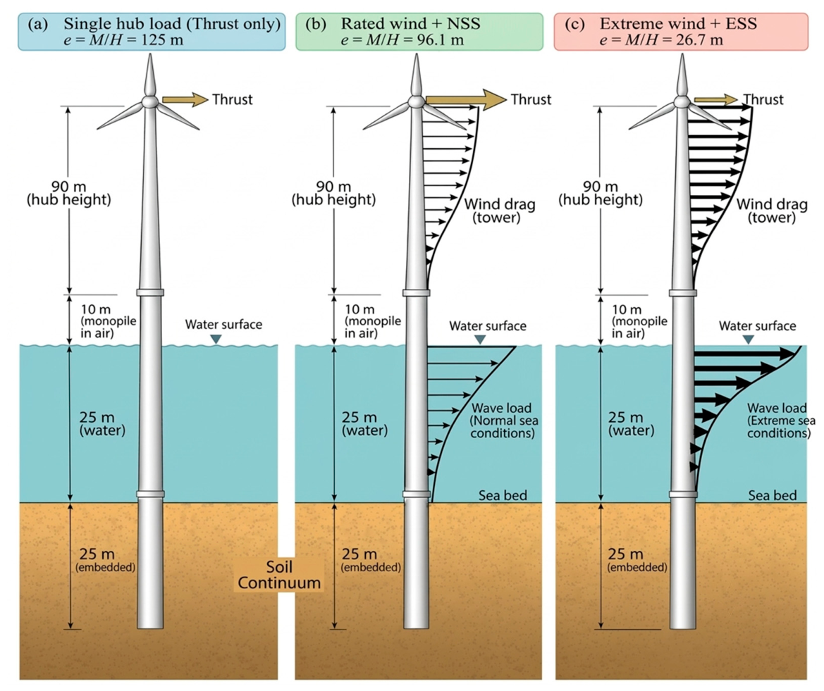
Table 4. Mudline load resultants and component contributions for the three loading scenarios.

Load case	H (MN)	M (GN·m)	e = M/H (m)	e/D	Hub thrust (MN)	Distributed (MN)
Single hub load	13.25	1.656	125.0	25.0	13.25	0
Rated wind + NSS	12.82	1.232	96.1	19.2	9.60	3.22
Extreme wind + ESS	35.48	0.946	26.7	5.3	5.14	30.34

Table 4. Mudline load resultants and component contributions for the three loading scenarios.

Load case	H (MN)	M (GN·m)	e = M/H (m)	e/D	Hub thrust (MN)	Distributed (MN)
Single hub load	13.25	1.656	125.0	25.0	13.25	0
Rated wind + NSS	12.82	1.232	96.1	19.2	9.60	3.22
Extreme wind + ESS	35.48	0.946	26.7	5.3	5.14	30.34

2.4. Nonlinear p–y Spring Model

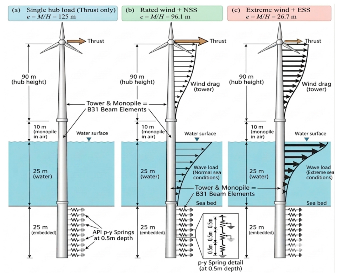
To test whether the conclusions depend on the soil idealization, each load case was also analyzed using a beam-on-nonlinear-Winkler-foundation model (Figure 7). The monopile was modelled with B31 beam elements having the same flexural rigidity, EI, as the corresponding solid monopile section in the continuum model. The p–y beam model extended from the embedded pile tip to the hub elevation, preserving the same 125 m load eccentricity above the mudline as in the continuum model. The 125 m hub elevation comprises 25 m of water depth, 10 m from still-water level to the tower base, and the 90 m NREL hub height measured above the tower base. The NREL tower itself is 87.6 m high. Accordingly, the environmental loads were applied at the same elevations as in the continuum model so that the spatial loading configuration and corresponding mudline force–moment resultants were preserved. Independent nonlinear springs were assigned at 0.5 m spacing along the embedded pile and followed the API static sand formulation (API, 2014) :

p = A p_u tanh[kz y/(A p_u)]

(11)

A = max(3 − 0.8z/D, 0.9)

(12)

where p_u is the ultimate resistance at depth z, governed by the shallow wedge or deep flow mechanism, and k is the initial modulus of subgrade reaction. The soil parameters are those of Table 3 with the same effective unit weight as the continuum model.

The nonlinear response was traced to mudline displacements exceeding 0.6 m using the modified Riks method. This ensured that both the serviceability and ultimate displacement levels defined in Section 2.5 were reached for all loading scenarios. As in the conventional API p–y formulation, no separate base-shear or base-moment reaction components were included, allowing the spring-model predictions to be compared with the continuum solution while retaining the assumptions of the conventional p–y framework.

Figure 7. Schematic of the nonlinear p–y spring model: beam-element monopile with independent API sand springs at 0.5 m spacing: (a) single hub load (e = 125.0 m); (b) rated wind + NSS (e = 96.1 m); (c) extreme wind + ESS (e = 26.7 m).

Figure 7. Schematic of the nonlinear p–y spring model: beam-element monopile with independent API sand springs at 0.5 m spacing: (a) single hub load (e = 125.0 m); (b) rated wind + NSS (e = 96.1 m); (c) extreme wind + ESS (e = 26.7 m).

2.5. Limit States and Post-Processing

To compare the load cases on the same deformation basis, responses were evaluated at two mudline lateral displacements: 0.10 m (y/D = 0.02) as a serviceability limit state (SLS) and 0.50 m (y/D = 0.10) as an ultimate limit state (ULS), following the displacement-based criteria commonly adopted for monopiles (Doherty and Gavin, 2012; Ma and Yang, 2023). These displacement levels are common response-comparison benchmarks and should not be interpreted as code-verified serviceability or ultimate design limits for the individual loading scenarios.

In the continuum model the full reference loads of Table 4 are reached at mudline displacements of 0.81, 0.53 and 0.56 m for the hub, NSS and ESS cases. Global quantities (horizontal load H, moment M and rotation θ) were interpolated to exactly 0.10 and 0.50 m. Profiles were extracted at the output increments closest to these displacements, and each profile was normalised by the mudline horizontal load of the same increment.

Depth z is measured downward from the mudline and normalised by L = 25 m. Deflection is normalised as u/D, bending moment as M/(HD), contact pressure as CPRESS·D²/H, and net soil reaction per unit length as pD/H. At the mudline

M/(HD) =e/D

(13)

so the normalization directly reflects the different effective load eccentricities among the three loading scenarios. In the continuum model, the net soil reaction p was obtained by integrating the interface normal and shear tractions around the pile circumference over each depth interval. The interface contact pressure, CPRESS is available only from the continuum model and should not be interpreted as equivalent to the nominal spring pressure p/D in the Winkler representation. The rotation point, z_r is defined as the depth at which the lateral pile deflection changes sign.

3. Results and Discussion

3.1. Global Response

Figure 8 shows the mudline horizontal load, overturning moment and rotation against mudline displacement for both the continuum and p–y modelling approaches. Because loading is proportional, M/H is constant throughout each analysis and equals the effective load height: 125.0 m for the hub load, 96.1 m for NSS and 26.7 m for ESS (Table 5). Under ESS the distributed, mainly hydrodynamic, component (30.3 MN) is about six times the hub thrust (5.1 MN). This brings the resultant down to approximately the still-water level, 25 m above the mudline. Under NSS the rotor thrust still provides about 75% of the horizontal load, so the resultant remains high on the structure. Similar dominance of rotor thrust under operating conditions and of wave load in extreme sea states has been reported for monopile-supported turbines (Arany et al., 2017; Det Norske Veritas, 2007; Shi et al., 2012)

The same qualitative effect of load distribution is observed in both modelling approaches. At equal mudline displacement, ESS requires substantially greater horizontal load than the hub-load case, while its corresponding overturning moment is lower.

Figure 8. Global response: (a) continuum-model lateral load; (b) continuum-model overturning moment; (c) continuum-model mudline rotation; (d) p–y-model lateral load; (e) p–y-model overturning moment; and (f) p–y-model mudline rotation.

Figure 8. Global response: (a) continuum-model lateral load; (b) continuum-model overturning moment; (c) continuum-model mudline rotation; (d) p–y-model lateral load; (e) p–y-model overturning moment; and (f) p–y-model mudline rotation.

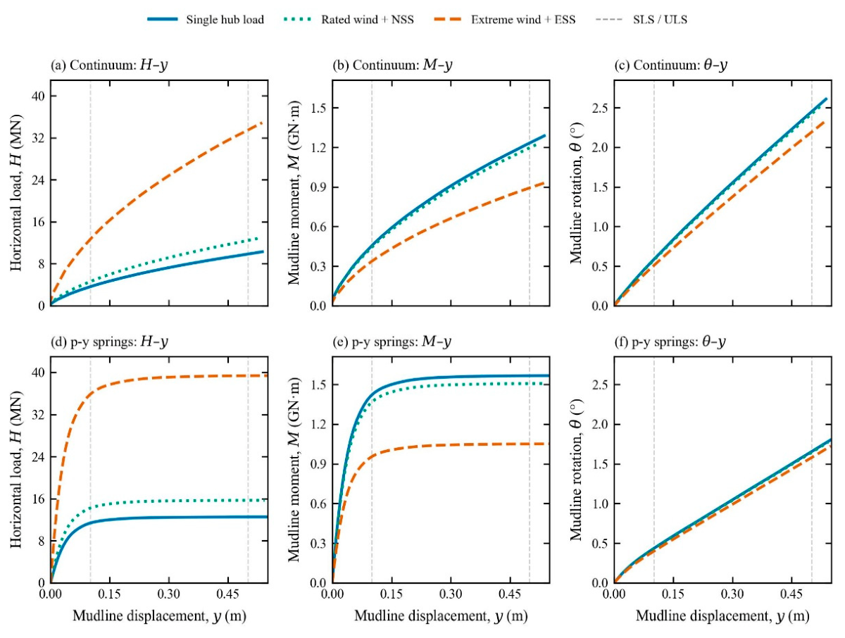
In the continuum model, the horizontal loads at SLS are 3.57, 4.52, and 12.40 MN for the hub, NSS, and ESS cases, respectively, and at ULS they are 9.83, 12.41, and 33.36 MN. The corresponding p–y values are 11.35, 14.21, and 35.77 MN at SLS and 12.53, 15.68, and 39.36 MN at ULS (Table 5). Figure 9 expresses these differences as ratios relative to the hub-load case. ESS requires approximately 3.4–3.5 times the horizontal load of the hub case in the continuum model and 3.1–3.2 times in the p–y model, while developing corresponding moment ratios of 0.72–0.74 and approximately 0.67, respectively. NSS requires about 1.25 times the horizontal load in both models, with a moment ratio of 0.96–0.97. These ratios change only slightly between SLS and ULS, indicating that the influence of load distribution is governed primarily by the applied force–moment load path rather than by the degree of soil nonlinearity.

Figure 9. Ratios of horizontal load (solid lines) and overturning moment (dotted lines) for the NSS and ESS cases relative to the single-hub-load case at the same mudline displacement: (a) continuum model; and (b) p–y model.

Figure 9. Ratios of horizontal load (solid lines) and overturning moment (dotted lines) for the NSS and ESS cases relative to the single-hub-load case at the same mudline displacement: (a) continuum model; and (b) p–y model.

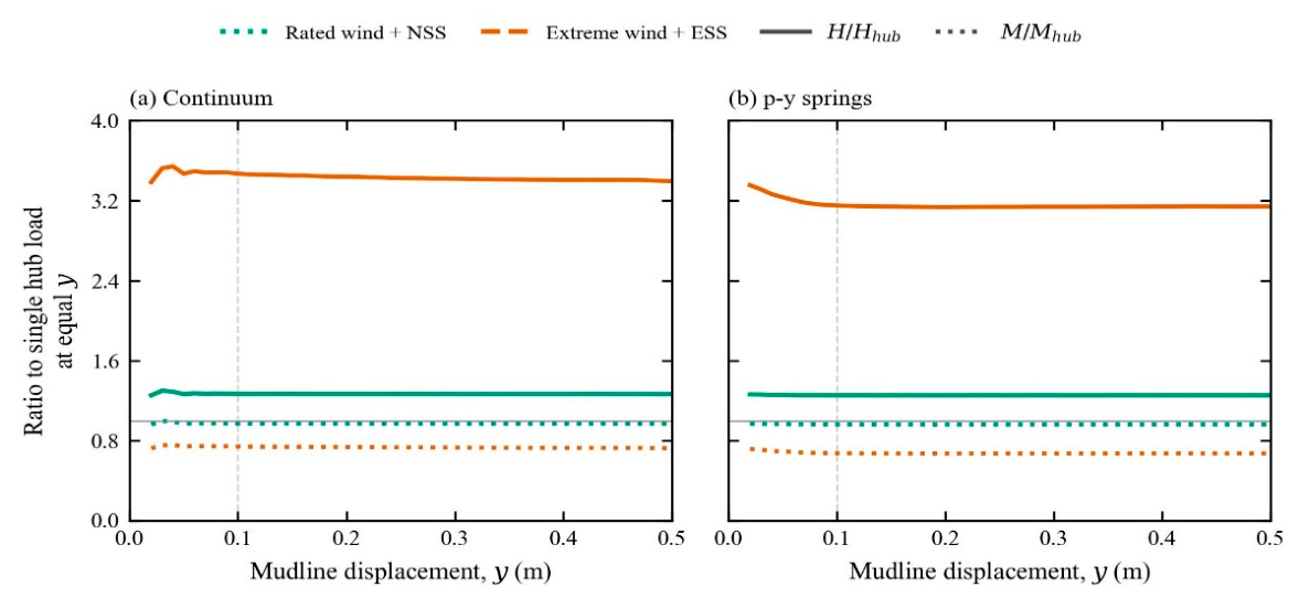
This behaviour is consistent with the mechanics of rigid piles, in which the lateral resistance at a given displacement depends on the combination of horizontal load and moment at the mudline, and therefore on the load eccentricity (Guo, 2008; Zhang et al., 2005) . A high-eccentricity load is more strongly moment-dominated. The soil resists mainly through a couple between the shallow soil in front of the pile and the soil near the toe, and the mudline displacement comes largely from rotation. A low-eccentricity load such as ESS is dominated by shear. It is resisted mostly by net horizontal resistance along the shaft, allowing greater horizontal resistance to be mobilized, so the same displacement requires a much larger horizontal load acting over a much shorter lever arm. (Lada et al., 2014) similarly reported that increasing the load eccentricity reduces the initial rotational stiffness of stiff monopiles and increases mudline displacement. NSS falls close to the hub case because rotor thrust still dominates its resultant.

Mudline rotation is less sensitive to load distribution (Figure 8c, f). At equal displacement, ESS reduces rotation by approximately 10–12% in the continuum model and by approximately 4–7% in the p–y model relative to the hub case, while NSS changes it by less than 1.5%. All cases remain predominantly rotation-dominated, consistent with the rigid-body behavior of monopiles with L/D ≈ 5 (Gupta and Basu, 2018; Klinkvort and Hededal, 2014; LeBlanc et al., 2010) , and ESS adds only a modest translational component.

3.2. Deformation Mode and Rotation Point

The normalised deflection profiles in Figure 10 show rigid-body rotation for every load case and both limit states. Deflection varies almost linearly with depth; changes sign once at the rotation point and reverses near the toe. Increasing the load level primarily changes the magnitude of deformation, while the normalized profile shape remains broadly similar. This rigid-body-dominated rotation agrees with the behaviour reported for semi-rigid and rigid monopiles in dense sand (LeBlanc et al., 2010; Ma and Yang, 2023) . The hub and NSS profiles practically coincide in both models, because about 75% of the NSS horizontal load is hub thrust.

Figure 10. Normalized pile deflection, u/D, against normalized depth, z/L: (a, b) continuum model at SLS and ULS, respectively; and (c, d) p–y model at SLS and ULS, respectively.

Figure 10. Normalized pile deflection, u/D, against normalized depth, z/L: (a, b) continuum model at SLS and ULS, respectively; and (c, d) p–y model at SLS and ULS, respectively.

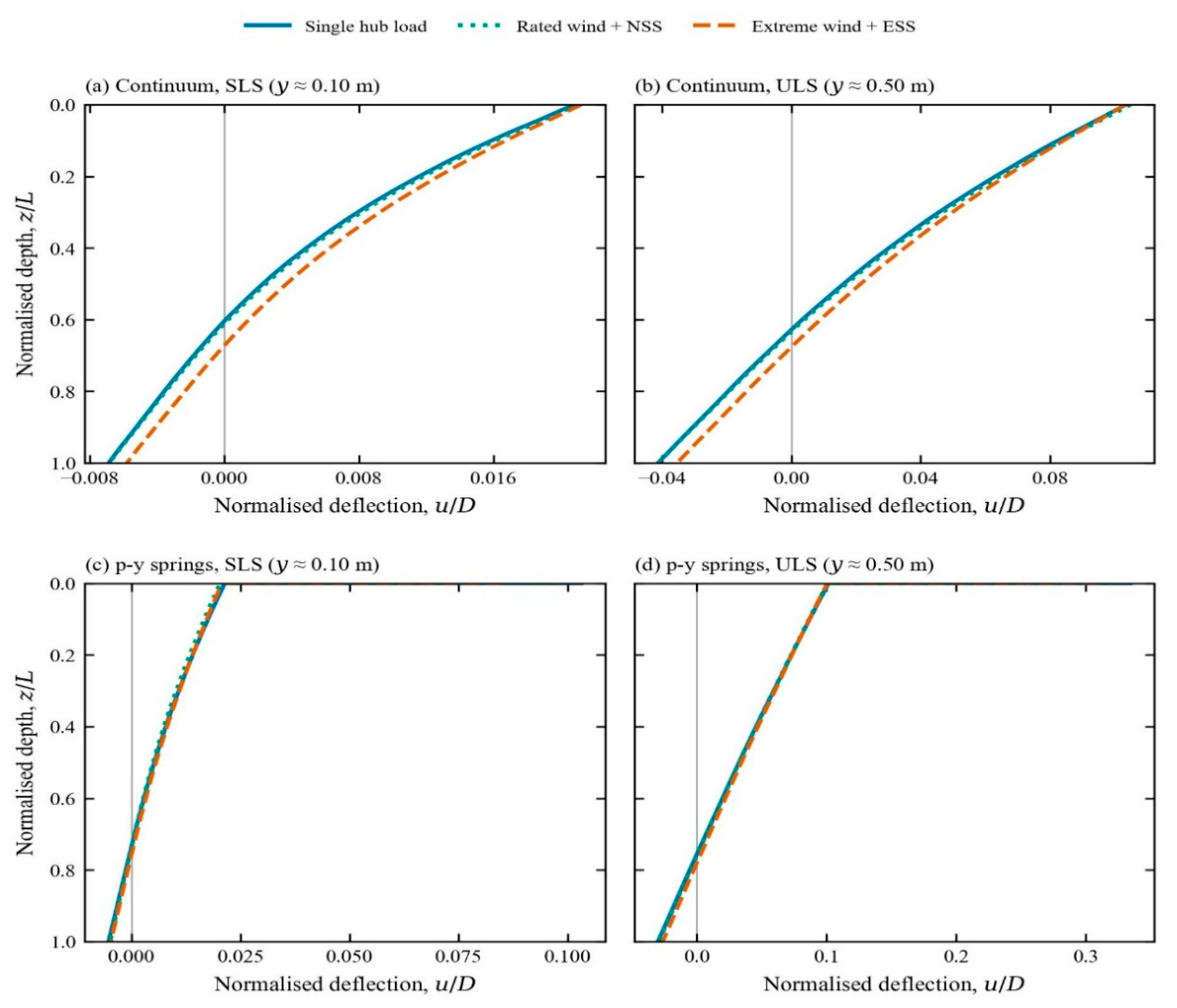
ESS moves the rotation point deeper in both modelling approaches (Figure 10; Figure 16c). In the continuum model, z_r/L is 0.601, 0.609 and 0.668 at SLS and 0.627, 0.633 and 0.675 at ULS for the hub, NSS and ESS cases, so the ESS rotation point lies 1.2–1.7 m deeper. In the p–y model, z_r/L is 0.734, 0.735 and 0.756 at SLS and 0.756, 0.759 and 0.780 at ULS, a deepening of 0.5–0.6 m.

Classical rigid-pile analyses predict the same trend: the rotation point moves toward the toe as load eccentricity decreases (Guo, 2008; Zhang et al., 2005). A shear-dominated load requires greater net forward resistance above the rotation point, and the pile accommodates this demand by rotating about a deeper point, thereby enlarging the zone over which passive soil resistance is mobilized in front of the pile. In all cases, the rotation point also deepens slightly from SLS to ULS as the shallow soil progressively yields and a greater proportion of resistance is mobilized at depth. The continuum-model rotation points (0.60–0.68L) are consistent with the range obtained in the validation against Ma and Yang (2023). The p–y model places the rotation points approximately 0.10–0.13L deeper than the continuum model.

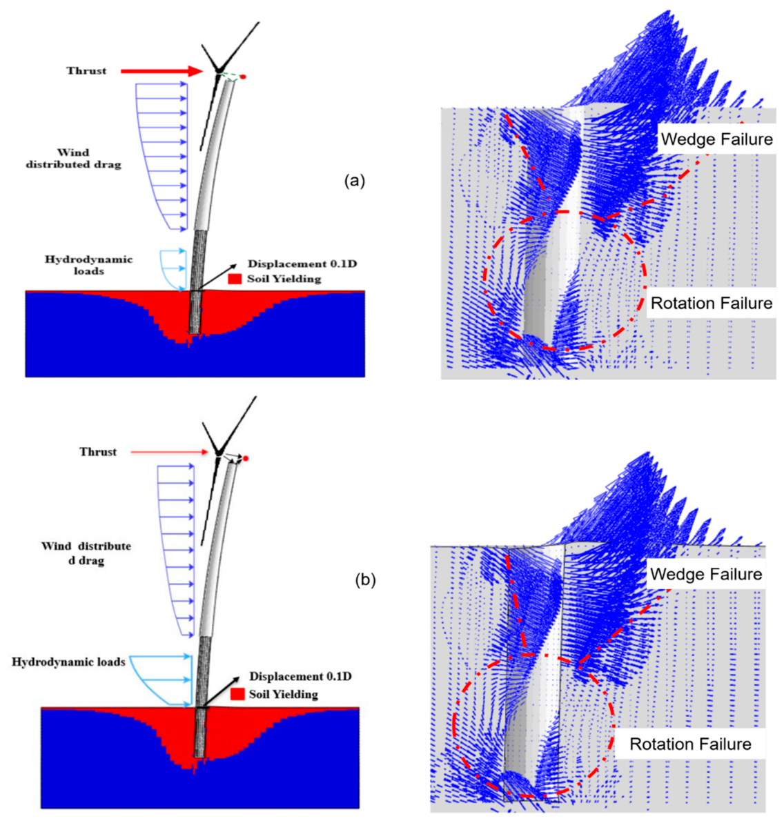
The soil deformation mechanisms at ULS are shown in Figure 11. Under both NSS and ESS loading, the soil exhibits a shallow wedge mechanism in front of the pile together with rotational soil flow around the pile toe, consistent with mechanisms reported for semi-rigid and rigid piles (Hong et al., 2017; Ma and Yang, 2023) .

Unlike the mechanism reported by (Ma and Yang, 2023), no distinct horizontal-flow zone was identified at intermediate depth in the present analyses. Under ESS, the large distributed wave load produces more extensive mobilization of the deeper soil and the soil around the pile toe.

Figure 11. Soil deformation mechanisms around the monopile at ULS: (a) rated wind + NSS; and (b) extreme wind + ESS.

Figure 11. Soil deformation mechanisms around the monopile at ULS: (a) rated wind + NSS; and (b) extreme wind + ESS.

3.3. Bending-Moment Distribution

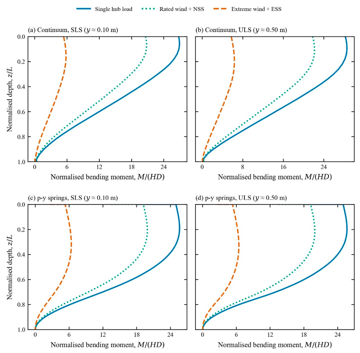
Figure 12 shows the bending moment normalized by HD. At the mudline M/(HD) is expected to correspond to e/D, so the profiles separate primarily according to effective eccentricity: 25.0, 19.2, and 5.3 for the hub, NSS, and ESS cases, respectively. Per unit horizontal load, the hub load case therefore imposes approximately five times the mudline bending demand of the ESS case. In every case, the bending moment peaks just below the mudline and decreases to nearly zero toward the toe, with no reverse bending, consistent with the response of a rigid pile (Gupta and Basu, 2018) .

Load distribution changes both the magnitude and the depth of the maximum bending moment (Figs. 12 and 16d). At equal mudline displacement, the ESS maximum moment is 21–25% lower than the hub-load value: 1.064 versus 1.409 GN·m in the continuum model at ULS, and 1.272 versus 1.608 GN·m in the p–y model. The location of the maximum moment also shifts downward under ESS. In the continuum model, its depth increases from 1.5 to 3.5 m below the mudline at SLS and from 2.5 to 4.5 m at ULS. In the p–y model, it increases from 4.5 to 8.0 m at SLS and from 5.0 to 8.5 m at ULS. The maximum moment occurs where the pile shear force becomes zero, that is, where the cumulative soil reaction balances the applied horizontal load (Guo, 2008) .

Under a high-eccentricity load, the horizontal shear is small relative to the overturning moment, so the zero-shear point lies relatively close to the mudline. Under ESS, the horizontal shear is much larger relative to moment, and a greater depth of mobilized soil resistance is required to balance it. The ESS bending-moment profile also decays more gradually with depth, consistent with the more distributed soil-reaction mobilization discussed in Section 3.5. Therefore, representing the extreme condition by a single high-eccentricity hub load would overestimate the moment-to-shear ratio transferred to the foundation and predict the critical bending section at a shallower depth.

Figure 12. Normalized bending moment M/(HD) against normalized depth z/L: (a, b) continuum model at SLS and ULS , respectively; (c, d) p–y model at SLS and ULS, respectively;.

Figure 12. Normalized bending moment M/(HD) against normalized depth z/L: (a, b) continuum model at SLS and ULS , respectively; (c, d) p–y model at SLS and ULS, respectively;.

3.4. Earth Pressure Distribution

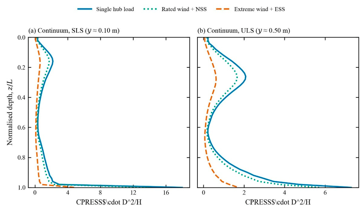
Figure 13 shows the normalised pile-soil contact pressure CPRESS·D²/H along the pile. In every case resistance is mobilised in two zones: a shallow peak associated with the passive wedge in front of the pile, and a concentration near the toe associated with rotation of the lower pile. This is the typical distribution for semi-rigid and rigid piles, and similar distributions were reported by (Hong et al., 2017; Ma and Yang, 2023) .

The hub and NSS cases nearly coincide and exhibit the highest normalized pressure peaks. Their relatively high load eccentricities produce a more moment-dominated response, resulting in strong shallow resistance together with pronounced contact-pressure mobilisation near the lower pile. By contrast, the ESS case consistently exhibits lower normalized peaks and a less pronounced shallow concentration. Because ESS is more shear-dominated, the soil resistance is distributed over a larger portion of the embedded pile rather than being concentrated as strongly in the shallow and toe regions. This behaviour is consistent with the deeper rotation point observed under ESS loading and the more distributed soil-reaction mechanism discussed in Section 3.5.

From SLS to ULS, the shallow pressure peak shifts downward from approximately z/L=0.16 to 0.27, indicating progressive mobilisation of deeper soil as the near-surface soil yields. The contact pressure on the passive side of the pile is substantially greater than that on the opposite side, by a factor of approximately 3.5 for the hub and NSS cases and approximately 2.8 for ESS. This difference further demonstrates the asymmetric soil mobilisation associated with lateral pile movement.

The pronounced contact-pressure concentration near the toe highlights the importance of lower-pile and base interaction for monopiles with relatively small L/D. As the pile rotates, the lower portion moves in the opposite direction to the upper pile, generating substantial soil resistance near the toe. Such lower-pile and base effects are represented explicitly in the PISA framework through additional base-shear and base-moment components (Burd et al., 2019; Byrne et al., 2017). Overall, the results show that reducing the effective load eccentricity from the hub-load condition to the wave-dominated ESS condition redistributes the normalized soil-contact resistance from concentrated shallow and toe reactions toward a more distributed resistance along the embedded pile.

Figure 13. Normalized soil-pile contact pressure CPRESS·D²/H against normalized depth z/L from the continuum model at: (a) SLS and (b) ULS.

Figure 13. Normalized soil-pile contact pressure CPRESS·D²/H against normalized depth z/L from the continuum model at: (a) SLS and (b) ULS.

3.5. Soil-Reaction Mobilization and Local p–y Response

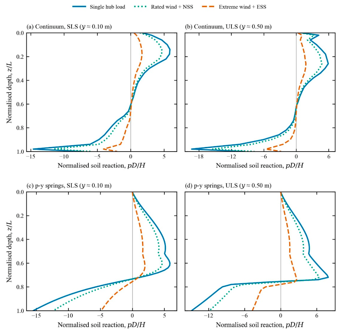
Figure 14 shows the normalised net soil reaction pD/H. In every case it has two lobes: forward resistance above the rotation point and a reversed reaction concentrated near the toe, with the zero crossing at the rotation point. This confirms the rigid behaviour identified in the deflection profiles.

Load distribution controls how the resistance is split between the two zones. Under the hub and NSS loads the toe reaction dominates. In the continuum model, pD/H near the toe (z = 24.5 m) is −14.2 and −11.2 at SLS and −18.9 and −15.0 at ULS, whereas under ESS it is only −3.9 at SLS and −5.5 at ULS. The p–y model gives the same ranking: −14.7, −11.7 and −4.6 at SLS.

Per unit horizontal load, ESS also mobilises a lower and more uniform forward reaction above the rotation point. The resistance mechanism therefore changes from a moment-resisting couple between the shallow front soil and the toe under hub-type loading to a predominantly distributed shear resistance under ESS. Because the profiles are normalized by H, however, the lower normalized ESS values should not be interpreted as lower absolute soil resistance; the absolute ESS reactions remain the largest because the applied horizontal load is much greater.

In the upper part of the pile the shape of the reaction profile depends on the modelling approaches. In the continuum model, forward resistance peaks at z/L ≈ 0.15–0.26 and decreases towards the rotation point. In the p–y model it keeps increasing with depth almost to the rotation point, because the API ultimate resistance increases with depth and is reached at small displacements. The load-case ranking, however, is the same in both models. Despite these differences in profile shape, the load-case ranking remains the same in both approaches.

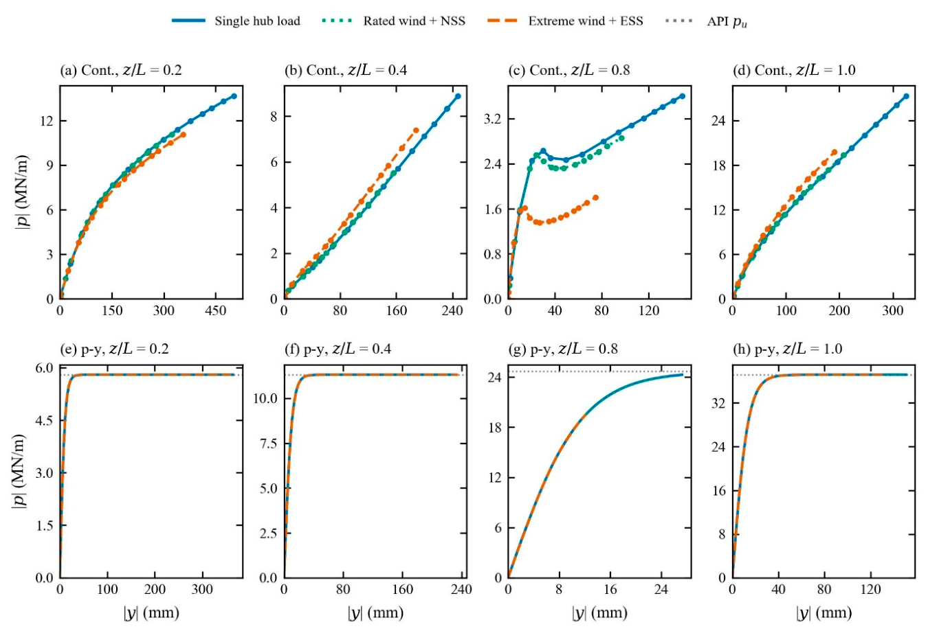
Figure 15 compares the local soil response at four normalized depths. In the p–y model, each spring follows the same prescribed backbone relation regardless of load case. Load distribution therefore changes only the position reached along the same local p–y curve. At ULS, the springs from the mudline to approximately 13 m depth, together with the toe-region springs, have reached or closely approached the prescribed ultimate resistance for all three load cases.

Figure 14. Normalized net soil reaction pD/H against normalized depth z/L: (a, b) continuum model at SLS and ULS; (c, d) p–y model at SLS and ULS.

Figure 14. Normalized net soil reaction pD/H against normalized depth z/L: (a, b) continuum model at SLS and ULS; (c, d) p–y model at SLS and ULS.

In the continuum model the local response depends on the load case. At z = 20 m (0.8L, just below the rotation point), ESS mobilises about 1.4–1.8 MN/m compared with 2.5–3.5 MN/m for the hub load at similar local displacements, and at z = 10 m the ESS response is slightly stiffer.

Previous studies (Klinkvort and Hededal, 2014) , found that the normalised ultimate soil resistance was unaffected by load eccentricity for e/D = 8.25–17.75. The present ESS case (e/D = 5.3) lies below that range, and the load-case dependence appears mainly near the rotation point, where the local soil movement is governed by the balance between rotation and translation. The continuum results therefore suggest that, under strongly wave-dominated low-eccentricity loading, the local reaction cannot be described solely by displacement magnitude; it is also influenced by the global deformation mode. Independent one-dimensional p–y springs cannot represent this coupling explicitly. Depth- and rotation-dependent reaction components, such as those incorporated in the PISA framework (Burd et al., 2019; Byrne et al., 2019) , provide one possible route for representing this behaviour.

Figure 15. Local soil reaction |p| against local pile displacement |y| at z/L = 0.2, 0.4, 0.8 and 1.0: (a–d) continuum model, relative to the geostatic state; (e–h) p–y model, with dotted lines indicating the API ultimate resistance p_u.

Figure 15. Local soil reaction |p| against local pile displacement |y| at z/L = 0.2, 0.4, 0.8 and 1.0: (a–d) continuum model, relative to the geostatic state; (e–h) p–y model, with dotted lines indicating the API ultimate resistance p_u.

3.6. Cross-Model Consistency and Model-Dependent Response

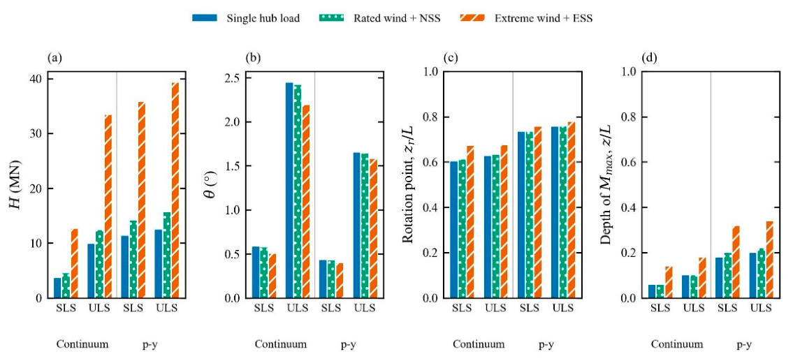
Figure 16 and Table 5 summarize the principal global and local response metrics. Several effects are consistently reproduced by both modelling approaches. At the same mudline displacement, ESS requires approximately 3.1–3.5 times the horizontal load of the hub case while developing only about 0.7 times its overturning moment. ESS also reduces mudline rotation, shifts the rotation point downward, moves the maximum bending moment to greater depth and produces lower normalised toe reaction in the extracted profiles. NSS remains close to the hub-load case for most normalized response measures. These common trends indicate that the principal effects of load distribution are reproduced consistently by both soil–pile interaction formulations and are therefore not artifacts of a single modelling approach.

Other response characteristics, however, are strongly model-dependent. At SLS, the p–y model required approximately 2.9–3.2 times the horizontal load of the continuum model to reach the same mudline displacement. The p–y response had already mobilised approximately 91% of the horizontal load reached by the same p–y analysis at y = 0.50 m, whereas the continuum response continued to harden beyond 0.50 m.

The p–y model also predicted a deeper rotation point (0.73–0.78L compared with 0.60–0.68L in the continuum model), a deeper maximum-moment location, a 23–33% smaller mudline rotation, and a different shallow soil-reaction profile. The greater stiffness and earlier mobilisation of limiting resistance in the p–y model are consistent with previous studies reporting that conventional API sand p–y curves can overpredict the initial lateral stiffness of large-diameter monopiles (Choo et al., 2014; Choo and Kim, 2015; Doherty and Gavin, 2012; Thieken et al., 2015).

Differences between the two modelling approaches may also be influenced by the conventional p–y formulation not including independent base-shear and base-moment components, which have been shown to contribute to the response of rigid and low-L/D monopiles (Burd et al., 2019; Byrne et al., 2019; Taborda et al., 2019) .

Overall, the comparison separates two aspects of the response. First, the direction and relative magnitude of the load-distribution effects are reproduced consistently by both modelling approaches: compared with the hub-load case, ESS requires substantially greater horizontal load at the same displacement, develops lower moment demand, produces smaller mudline rotation, shifts the rotation point downward, and moves the maximum bending moment deeper. Second, the absolute stiffness, rotation depth, bending-moment location, and local soil-reaction distribution remain sensitive to the adopted soil–pile interaction formulation. The continuum and p–y models therefore provide consistent evidence for the influence of load distribution, while differing in the predicted magnitude and spatial distribution of the soil–foundation response.

Table 5. Global and local response quantities at SLS (y = 0.10 m) and ULS (y = 0.50 m).

Model	Case	State	H (MN)	M (GN·m)	θ (°)	zr/L	Mmax (GN·m)	z(Mmax) (m)
Continuum	Hub	SLS	3.57	0.447	0.59	0.601	0.490	1.5
	NSS	SLS	4.52	0.435	0.58	0.609	0.480	1.5
	ESS	SLS	12.40	0.331	0.52	0.668	0.368	3.5
	Hub	ULS	9.83	1.229	2.46	0.627	1.409	2.5
	NSS	ULS	12.41	1.193	2.43	0.633	1.381	2.5
	ESS	ULS	33.36	0.890	2.21	0.675	1.064	4.5
p–y	Hub	SLS	11.35	1.419	0.43	0.734	1.474	4.5
	NSS	SLS	14.21	1.365	0.43	0.735	1.421	5.0
	ESS	SLS	35.77	0.954	0.40	0.756	1.156	8.0
	Hub	ULS	12.53	1.566	1.65	0.756	1.608	5.0
	NSS	ULS	15.68	1.506	1.64	0.759	1.564	5.5
	ESS	ULS	39.36	1.050	1.58	0.780	1.272	8.5

Table 5. Global and local response quantities at SLS (y = 0.10 m) and ULS (y = 0.50 m).

Model	Case	State	H (MN)	M (GN·m)	θ (°)	zr/L	Mmax (GN·m)	z(Mmax) (m)
Continuum	Hub	SLS	3.57	0.447	0.59	0.601	0.490	1.5
	NSS	SLS	4.52	0.435	0.58	0.609	0.480	1.5
	ESS	SLS	12.40	0.331	0.52	0.668	0.368	3.5
	Hub	ULS	9.83	1.229	2.46	0.627	1.409	2.5
	NSS	ULS	12.41	1.193	2.43	0.633	1.381	2.5
	ESS	ULS	33.36	0.890	2.21	0.675	1.064	4.5
p–y	Hub	SLS	11.35	1.419	0.43	0.734	1.474	4.5
	NSS	SLS	14.21	1.365	0.43	0.735	1.421	5.0
	ESS	SLS	35.77	0.954	0.40	0.756	1.156	8.0
	Hub	ULS	12.53	1.566	1.65	0.756	1.608	5.0
	NSS	ULS	15.68	1.506	1.64	0.759	1.564	5.5
	ESS	ULS	39.36	1.050	1.58	0.780	1.272	8.5

Figure 16. Comparison of key response parameters at SLS and ULS for Continuum and p-y spring modelling approaches (a) horizontal load at the target mudline displacement; (b) mudline rotation; (c) normalized rotation-point depth; and (d) depth of maximum bending moment.

Figure 16. Comparison of key response parameters at SLS and ULS for Continuum and p-y spring modelling approaches (a) horizontal load at the target mudline displacement; (b) mudline rotation; (c) normalized rotation-point depth; and (d) depth of maximum bending moment.

4. Engineering Implications

The results indicate that the resulting mudline force–moment load path and effective load height should be represented explicitly when assessing large-diameter monopiles under wave-dominated conditions. In the ESS case, replacing the prescribed low-eccentricity ESS load path with a high-eccentricity hub load changes the force–moment combination acting at the mudline. Because no matched point-load analysis was performed at the same effective height as ESS, the present study does not isolate the effect of spatial distribution shape from the effect of resultant eccentricity. Consequently, for the same displacement or rotation criterion, the simplified hub-load representation would not only misrepresent the magnitude of the global foundation demand, but would also alter the predicted depth over which soil resistance is mobilized, the rotation point, and the location of the critical bending section.

By contrast, under thrust-dominated operating conditions, such as the rated-wind case combined with a normal sea state, the single hub-load representation provides a closer approximation to the realistic distributed-loading response. Because rotor thrust contributes approximately 75% of the total horizontal load in the NSS case, the effective load eccentricity remains relatively high and the normalized deformation, bending-moment, and soil-reaction profiles remain close to those obtained for the hub-load case. Nevertheless, the hub-load case requires a lower mudline horizontal load than the NSS case to reach the same displacement. It can therefore provide a reasonable approximation of the response mechanism under thrust-dominated conditions, but it does not reproduce the absolute global load demand exactly.

The results also indicate that the depth of peak bending demand is sensitive to the prescribed mudline force–moment combination. Under the low-eccentricity ESS load path, the extracted peak occurs deeper than under the high-eccentricity hub-load condition. This indicates that load distribution should be considered when selecting the depth of wall-thickness transitions or other changes in monopile sectional properties, because an idealized hub load may place the predicted maximum bending demand too close to the mudline and therefore misidentify the structurally critical embedded region.

Finally, the comparison between the continuum and p–y approaches shows that the conventional API p–y formulation reproduces the principal direction of the load-distribution effects, including the larger horizontal resistance associated with ESS, the deeper rotation point, and the downward shift of the maximum bending moment. However, the p–y model predicts substantially greater stiffness, earlier mobilisation of limiting resistance, and different local reaction distributions compared with the continuum model. Accordingly, the differences in absolute stiffness and reaction distribution should be interpreted as formulation-dependent until the API inputs and calibration range are verified; benchmarking or calibrating the p–y formulation itself is outside the primary scope of this study (Choo and Kim, 2015; Doherty and Gavin, 2012; Thieken et al., 2015) . The results therefore support using realistic distributed environmental loads together with a soil–pile interaction formulation appropriate to the required level of response prediction, rather than relying on a single equivalent hub load combined with an uncalibrated conventional p–y representation.

5. Limitations and Future Work

The analyses consider static, monotonic, proportional loading. Cyclic accumulation of rotation (Achmus et al., 2009; LeBlanc et al., 2010) , dynamic amplification, wind–wave misalignment and the time-varying phasing of wind and wave loads are not included. Only one pile geometry (D = 5 m, L/D = 5) and one homogeneous dense sand are studied. The serviceability and ultimate states are defined by mudline displacement, rather than by case-specific design load levels.

The p–y model uses uncalibrated API static-sand springs without independent base-shear or base-moment resistance, while the continuum-derived soil reaction depends on the procedure used to integrate the pile–soil interface stresses. The continuum and p–y formulations should therefore be interpreted as two alternative soil–pile interaction representations rather than as equivalent models of the same local soil-response mechanism.

Future work should include single concentrated loads applied at the effective resultant heights of the realistic environmental load cases to separate the influence of load-distribution shape from that of the resultant height. This comparison would distinguish whether the observed response differences arise primarily from the reduced eccentricity of the environmental resultant or from the spatial distribution of loading itself. Future studies should also consider cyclic and dynamic loading, wind–wave directional misalignment and phase relationships, other monopile diameters and embedment ratios, layered and heterogeneous soil profiles, and soil-reaction formulations calibrated against continuum analyses and, where available, field or physical-model measurements.

6. Conclusions

The effect of realistic environmental load distribution on a 5 m-diameter monopile in dense sand supporting the NREL 5 MW turbine was investigated using a validated 3D coupled continuum model and a nonlinear p–y modelling approach. The main conclusions are:

(1)

Load distribution, expressed through the effective load height e=M/H, controls how the foundation demand is partitioned between horizontal load and overturning moment. At equal mudline displacement, ESS loading (e=26.7 m) required 3.4–3.5 times in the continuum model and 3.1–3.2 times in the p–y model the horizontal load of the hub load case (e=125 m), while developing only 0.67–0.74 of its overturning moment. These ratios changed only slightly between the serviceability and ultimate displacement states, indicating that the principal effect is associated with the applied force–moment load path rather than the deformation level alone.

(2)

The monopile exhibited predominantly rigid-body rotation under all load cases, with the continuum analysis showing a shallow soil-wedge mechanism and rotational flow around the toe. ESS loading shifted the rotation point downward, from approximately 0.60–0.63L to 0.67–0.68L in the continuum model, and also reduced the mudline rotation. The same downward shift of the rotation point was reproduced by the p–y model, although at greater normalized depths.

(3)

ESS loading reduced the maximum bending moment by approximately 21–25% and shifted its location deeper into the embedded pile, by about 2 m in the continuum model and 3.5 m in the p–y model at ULS. The hub-load idealisation therefore predicts the critical bending section at a shallower depth than the distributed ESS loading, demonstrating that realistic load distribution can influence the location of embedded structural detailing.

(4)

Under ESS loading, the soil-resistance mechanism shifted from a strongly moment-resisting couple between the shallow soil and the lower-pile/toe region toward a more uniformly distributed shear-resistance mechanism. The extracted normalised toe reaction was lower than in the hub-load case, while resistance was distributed over a larger portion of the embedded pile; the integrated reaction profile requires an equilibrium check before a quantitative ratio is retained.

(5)

Rated wind combined with a normal sea state produced a response close to that of the hub-load case in terms of deformation mode and normalized bending-moment and soil-reaction profiles. This similarity arises because rotor thrust contributes approximately 75% of the NSS horizontal load, maintaining a relatively high effective load eccentricity. However, the hub-load case still required approximately 20% less horizontal load than NSS at the same mudline displacement, indicating that the two cases are not equivalent in absolute global demand.

(6)

The principal load-distribution trends were reproduced by both modelling approaches, whereas the absolute stiffness, horizontal load required at a prescribed displacement, mudline rotation, rotation-point depth, maximum-moment depth, and local soil-reaction distribution depended on the adopted soil–pile interaction formulation.

The single-hub-load idealisation can therefore provide a reasonable approximation of the deformation mechanism under thrust-dominated operating conditions, but it does not adequately represent the force–moment combination, bending-demand distribution, or soil-resistance mobilisation under wave-dominated extreme loading. Accordingly, realistic distributed environmental loading should be represented explicitly when low-eccentricity wave loading contributes substantially to the foundation demand.

References

- Achmus, M., Kuo, Y.S., Abdel-Rahman, K., 2009. Behavior of monopile foundations under cyclic lateral load. Comput. Geotech. 36, 725–735. [CrossRef]
- Ahmed, S.S., Hawlader, B., 2016. Numerical Analysis of Large-Diameter Monopiles in Dense Sand Supporting Offshore Wind Turbines. International Journal of Geomechanics 16, 04016018. [CrossRef]
- API, R. 2GEO, 2014. Geotechnical and Foundation Design Considerations. Washington, DC.
- Arany, L., Bhattacharya, S., Macdonald, J., Hogan, S.J., 2017. Design of monopiles for offshore wind turbines in 10 steps. Soil Dynamics and Earthquake Engineering 92, 126–152. [CrossRef]
- Burd, H.J., Taborda, D.M.G., Zdravkovic, L., Abadie, C.N., Byrne, B.W., Houlsby, G.T., Gavin, K.G., Igoe, D.J.P., Jardine, R.J., Martin, C.M., McAdam, R.A., Pedro, A.M.G., Potts, D.M., 2019. PISA design model for monopiles for offshore wind turbines: application to a marine sand. Geotechnique 70, 1048–1066. [CrossRef]
- Byrne, B., McAdam, R., Burd, H., Houlsby, G., Martin, C., Beuckelaers, W., Zdravkovic, L., Taborda, D., Potts, D., Jardine, R., Ushev, E., Liu, T., Abadias Gomez, D., Gavin, K., Igoe, D., Doherty, P., Skov Gretlund, J., Pacheco Andrade, M., Muir Wood, A., Schroeder, F., 2017. PISA: new design methods for offshore wind turbine monopiles. Revue Française de Géotechnique 3. [CrossRef]
- Byrne, B.W., Houlsby, G.T., Burd, H.J., Gavin, K.G., Igoe, D.J.P., Jardine, R.J., Martin, C.M., McAdam, R.A., Potts, D.M., Taborda, D.M.G., Zdravkovic, L., 2019a. PISA design model for monopiles for offshore wind turbines: application to a stiff glacial clay till. Geotechnique 70, 1030–1047. [CrossRef]
- Byrne, B.W., McAdam, R.A., Burd, H.J., Beuckelaers, W.J.A.P., Gavin, K.G., Houlsby, G.T., Igoe, D.J.P., Jardine, R.J., Martin, C.M., Muirwood, A., Potts, D.M., Gretlund, J.S., Taborda, D.M.G., Zdravkovic, L., 2019b. Monotonic laterally loaded pile testing in a dense marine sand at Dunkirk. Geotechnique 70, 986–998. [CrossRef]
- Choo, Y.W., Kim, D., 2015. Experimental Development of the p-y Relationship for Large-Diameter Offshore Monopiles in Sands: Centrifuge Tests. Journal of Geotechnical and Geoenvironmental Engineering 142, 04015058. [CrossRef]
- Choo, Y.W., Kim, D., Park, J.H., Kwak, K., Kim, J.H., Kim, D.S., 2014. Lateral Response of Large-Diameter Monopiles for Offshore Wind Turbines from Centrifuge Model Tests. GEOTECHNICAL TESTING JOURNAL 37. [CrossRef]
- Coulomb, M., Coulomb, M., 2023. Essai sur une application des règles de Maximis & Minimis à quelques Problèmes de Statique, relatifs à l’Architecture. RFrG 175, 1. [CrossRef]
- Dassault Systèmes, 2017. Abaqus/CAE,Version 2017. Providence, RI, USA: Dassault Systèmes Simulia Corp. [WWW Document].
- Deng, Z.S., Xiao, Q., Yang, L., Liu, Y.C., Wang, E., 2025. Aeroelastic investigations of composite blade on floating offshore wind Turbine: Insights into stress responses on multi-hierarchy blade structures. Ocean Engineering 330, 121305. [CrossRef]
- Det Norske Veritas, 2007. DESIGN OF OFFSHORE WIND TURBINE STRUCTURES.
- Doherty, P., Gavin, K., 2012. Laterally loaded monopole design for offshore wind farms. Proceedings of Institution of Civil Engineers: Energy 165, 7–17. [CrossRef]
- Frohboese, P., Hassan, G., 2010. THRUST COEFFICIENTS USED FOR ESTIMATION OF WAKE EFFECTS FOR FATIGUE LOAD CALCULATION.
- Guo, W.D., 2008. Laterally loaded rigid piles in cohesionless soil. Canadian Geotechnical Journal 45, 676–697. [CrossRef]
- Gupta, B.K., Basu, D., 2018. Applicability of Timoshenko, Euler–Bernoulli and rigid beam theories in analysis of laterally loaded monopiles and piles. Geotechnique 68, 772–785. [CrossRef]
- Hong, Y., He, B., Wang, L.Z., Wang, Z., Ng, C.W.W., Mašín, D., 2017. Cyclic lateral response and failure mechanisms of semi-rigid pile in soft clay: centrifuge tests and numerical modelling. 54, 806–824. [CrossRef]
- IEC 61400-3-1, 2019. Wind energy generation systems – Part 3-1: Design requirements for fixed offshore wind turbines, International Electrotechnical Commission, Geneva, International Electrotechnical Commission. Geneva.
- Jawalageri, S., Bhattacharya, S., Jalilvand, S., Malekjafarian, A., 2024. A Comparative Study on Load Assessment Methods for Offshore Wind Turbines Using a Simplified Method and OpenFAST Simulations. Energies 2024, Vol. 17, Page 2189 17, 2189. [CrossRef]
- Jonkman, J., Buhl, M., 2005. FAST User’s Guide.
- Jonkman, J., Butterfield, S., Musial, W., Scott, G., 2009. Definition of a 5-MW Reference Wind Turbine for Offshore System Development. [CrossRef]
- Jonkman, J.M., 2007. Dynamics Modeling and Loads Analysis of an Offshore Floating Wind Turbine.
- Khezri, A., Park, H., Lee, D., 2024. Numerical Study on the Lateral Load Response of Offshore Monopile Foundations in Clay: Effect of Slenderness Ratio. Applied Sciences 2024, Vol. 14, Page 8366 14, 8366. [CrossRef]
- Klinkvort, R.T., Hededal, O., 2014. Effect of load eccentricity and stress level on monopile support for offshore wind turbines. Canadian Geotechnical Journal 51, 966–974. [CrossRef]
- Kong, D., Zhu, J., Long, Y., Zhu, B., Yang, Q., Gao, Y., Chen, Y., 2022. Centrifuge modelling on monotonic and cyclic lateral behaviour of monopiles in kaolin clay. Geotechnique 72, 661–674. [CrossRef]
- Lada, A.;, Ibsen, L., Bo, ;, Nicolai, G., 2014. The stiffness change and the increase in the ultimate capacity for a stiff pile resulting from a cyclic loading.
- Lai, Y., Wang, L., Hong, Y., He, B., 2020. Centrifuge modeling of the cyclic lateral behavior of large-diameter monopiles in soft clay: Effects of episodic cycling and reconsolidation. Ocean Engineering 200, 107048. [CrossRef]
- LeBlanc, C., Houlsby, G.T., Byrne, B.W., 2010. Response of stiff piles in sand to long-term cyclic lateral loading. Geotechnique 60, 79–90. [CrossRef]
- Lesny, K., Wiemann, J., 2006. Finite-Element-Modelling of Large Diameter Monopiles for Offshore Wind Energy Converters. GeoCongress 2006: Geotechnical Engineering in the Information Technology Age 2006, 1–6. [CrossRef]
- Ma, Y., Yang, J., 2023. Earth pressure distribution on laterally loaded offshore monopiles. Ocean Engineering 273, 113954. [CrossRef]
- Matlock, H., 1970. Correlations for design of laterally loaded piles in soft clay. Proceedings of the Annual Offshore Technology Conference 1970-April. [CrossRef]
- Mazzoni, S., Mckenna, F., Scott, M.H., Fenves, G.L., Iii, A., 2006. Open System for Earthquake Engineering Simulation (OpenSees) OpenSees Command Language Manual.
- Mohr, 1882. Mohr, O., “Ueber die Darstellung des Span-nungszustandes und des Deformationszustandes eines Kr-perelementes und über die Anwendung derselben in der Fes-tigkeitslehre,” Civilengenieur, Vol. 28, 1882, pp.113-56. - References - Scientific Research Publishi… [WWW Document]. URL https://www.scirp.org/reference/referencespapers?referenceid=107127 (accessed 10.13.26).
- Morison, J.R., Johnson, J.W., Schaaf, S.A., Morison, J.R., Johnson, J.W., Schaaf, S.A., Morison, R., J., Johnson, W., J., Schaaf, A., S., 1950. The Force Exerted by Surface Waves on Piles. JPetT 2, 149–154. [CrossRef]
- MSC Software, n.d. Adams Multibody Dynamics Simulation Cadence [WWW Document]. URL https://www.cadence.com/en_US/home/tools/msc-software/adams.html (accessed 10.16.26).
- Murphy, G., Igoe, D., Doherty, P., Gavin, K., 2018. 3D FEM approach for laterally loaded monopile design. Comput. Geotech. 100, 76–83. [CrossRef]
- Noh, Y.J., Sun, M., 2025. Environmental contours using copulas for extreme load estimate of offshore wind turbines. Ocean Engineering 326, 120919. [CrossRef]
- Reese, L.C., Cox, W.R., Koop, F.D., 1974. Analysis of Laterally Loaded Piles in Sand. Proceedings of the Annual Offshore Technology Conference 1974-May, 473–480. [CrossRef]
- Sadiq, S., Kim, H.J., Won, M.S., Park, Y.C., 2025a. A qualitative study on the lateral behavior of rock-socketed monopiles. Marine Structures 104, 103892. [CrossRef]
- Sadiq, S., Won, M.S., Kim, H.J., Hong, C., 2025b. Hybrid finite element and machine learning approach for estimating lateral capacity of partially rock-socketed monopiles. Ocean Engineering 330, 121286. [CrossRef]
- Shi, W., Park, H.C., Baek, J.H., Kim, C.W., Kim, Y.C., Shin, H.K., 2012. Study on the marine growth effect on the dynamic response of offshore wind turbines. International Journal of Precision Engineering and Manufacturing 2012 13:7 13, 1167–1176. [CrossRef]
- Suryasentana, S.K., Lehane, B.M., 2016. Updated CPT-based p–y formulation for laterally loaded piles in cohesionless soil under static loading. Geotechnique 66, 445–453. [CrossRef]
- Taborda, D.M.G., Zdravkovic, L., Potts, D.M., Burd, H.J., Byrne, B.W., Gavin, K.G., Houlsby, G.T., Jardine, R.J., Liu, T., Martin, C.M., McAdam, R.A., 2019. Finite-element modelling of laterally loaded piles in a dense marine sand at Dunkirk. Geotechnique 70, 1014–1029. [CrossRef]
- Thieken, K., Achmus, M., Lemke, K., Terceros, M., 2015. Evaluation of p-y Approaches for Large-Diameter Monopiles in Sand. International Journal of Offshore and Polar Engineering 25, 134–144. [CrossRef]
- Wang, L., Lai, Y., Hong, Y., Mašín, D., 2020. A unified lateral soil reaction model for monopiles in soft clay considering various length-to-diameter (L/D) ratios. Ocean Engineering 212, 107492. [CrossRef]
- Wind Europe, 2021. Offshore wind in Europe - key trends and statistics 2020. Wind Europe, Brussels, Belgium. [WWW Document]. URL Wind Europe, Brussels, Belgium. (accessed 10.16.26).
- Zdravkovic, L., Taborda, D.M.G., Potts, D.M., Abadias, D., Burd, H.J., Byrne, B.W., Gavin, K.G., Houlsby, G.T., Jardine, R.J., Martin, C.M., McAdam, R.A., Ushev, E., 2019. Finite-element modelling of laterally loaded piles in a stiff glacial clay till at Cowden. Geotechnique 70, 999–1013. [CrossRef]
- Zhang, L., Silva, F., Grismala, R., 2005. Ultimate Lateral Resistance to Piles in Cohesionless Soils. Journal of Geotechnical and Geoenvironmental Engineering 131, 78–83. [CrossRef]
Disclaimer/Publisher’s Note: The statements, opinions and data contained in all publications are solely those of the individual author(s) and contributor(s) and not of MDPI and/or the editor(s). MDPI and/or the editor(s) disclaim responsibility for any injury to people or property resulting from any ideas, methods, instructions or products referred to in the content. |
© 2026 by the authors. Licensee MDPI, Basel, Switzerland. This article is an open access article distributed under the terms and conditions of the Creative Commons Attribution (CC BY) license (http://creativecommons.org/licenses/by/4.0/).
Copyright: This open access article is published under a Creative Commons CC BY 4.0 license, which permit the free download, distribution, and reuse, provided that the author and preprint are cited in any reuse.