

Submitted:
04 November 2026
Posted:
05 November 2026
You are already at the latest version
Abstract
The misrepresentation of frozen-thawed meat as fresh constitutes economic fraud that can result in financial losses and erode consumer confidence in meat products. Portable near-infrared (NIR) spectroscopy could serve as a process analytical tool for on-site screening if its predictive performance can be maintained across previously unseen animals. This study developed a leakage-controlled, explainable and reliability-calibrated workflow to screen chevon (goat meat) for freeze-thaw history with a handheld short-wave NIR spectrometer (710 to 1027 nm). Longissimus dorsi samples from 400 Black Bengal goats were scanned fresh and after vacuum-packed storage at −18 °C for 60 d and thawing. All data-driven steps used 320 training animals, nested animal-grouped cross-validation estimated performance and 80 unseen animals formed an independent test set. Freeze-thaw increased absorbance by 0.137 AU on average (median paired dz = 1.06) and changed spectral shape regionally. A support vector machine selected by the one-standard-error rule reached a nested accuracy of 0.865 ± 0.022 and a test accuracy of 0.888 (95% CI 0.831 to 0.931, AUC 0.961), equivalent to linear models. Discrimination relied mainly on the broadband absorbance level. At 95% confidence, class-conditional conformal prediction classified 56.2% of test samples with 98.9% accuracy and referred the remainder. Since the two states were scanned on different days, same-session validation is required before deployment. These results highlight the potential of handheld NIR spectroscopy for reliable on-site screening of freeze-thaw history in chevon.
Keywords:
near-infrared spectroscopy
; process analytical technology
; chevon
; food authentication
; explainable artificial intelligence
; machine learning
; nested cross-validation
1. Introduction
Goat meat, also known as chevon, constitutes an important red meat in Asia and Africa and holds considerable dietary importance in many communities [1]. Although freezing improves storage stability, ice crystal formation disrupts myofibrillar structures and increases drip loss while accelerating lipid and protein oxidation. These physicochemical changes make thawed meat lighter and less red and reduce its water-holding capacity [2]. The lower economic value and greater spoilage susceptibility of thawed meat compared with chilled meat create opportunities for its fraudulent sale as fresh. Previous European surveys documented that 8 to 15% of meat samples were incorrectly labeled as chilled [3]. Enzymatic, histological and biochemical approaches can identify previous freeze-thaw exposure, but their applicability remains limited by destructive testing, lengthy analytical procedures and susceptibility to variation in species, muscle type and processing conditions [3,4].
Near-infrared (NIR) spectroscopy coupled with machine learning has emerged as a rapid, non-destructive approach for authenticating foods of animal origin [5,6,7]. The availability of handheld spectrometers at prices below USD 1,000 enables measurements at the point of sale, although their restricted spectral coverage and relatively modest signal-to-noise ratios may limit analytical performance [8]. Previous studies have reported high classification accuracies for freeze-thaw detection across different meat and fish species. Handheld NIR spectroscopy achieved accuracies exceeding 95% in chicken fillets [9], while two low-cost devices achieved 90.3% and 94.1% accuracy in mackerel [10]. Higher accuracies have also been reported using NIR spectroscopy operating at 950 to 1700 nm for Spanish mackerel (97.8%) [11] and hyperspectral imaging for distinguishing fresh, temperature-abused and frozen-thawed beef (96.57%) [12].
The reported classification accuracies demonstrate the potential of spectroscopic approaches for freeze-thaw detection, but their applicability to routine inspection of previously unseen animals remains uncertain. A major concern is the validation strategy, as replicate spectra from the same sample are highly similar but are frequently distributed randomly between training and test sets. In the beef study, for instance, 4,950 spectra were randomly assigned to training (80%) and test (20%) sets [12]. When spectra originating from the same sample are distributed across both sets or model-tuning decisions influence test-set performance, the resulting accuracy may be artificially elevated. Data leakage of this nature has been associated with overoptimistic conclusions in machine-learning-based research [13,14]. Comparisons between fresh and frozen-thawed meat obtained from different animals introduce an additional confounding effect, as treatment differences cannot be separated from inherent between-animal variation. Further limitations concern model interpretation and prediction reliability. Although explanation methods are increasingly applied to spectroscopic data [15], strong correlations between neighboring wavelengths can compromise feature attribution, while permutation importance may generate unrealistic spectral combinations [16]. Wavelength markers identified using a single model and data partition may capture broadband baseline variation or noise near the spectral limits of compact spectrometers rather than chemical changes associated with freeze-thaw exposure. Conventional classifiers also provide a single class label without quantifying sample-level uncertainty, limiting an inspector’s ability to assess prediction reliability. Conformal prediction provides an approach to uncertainty assessment by constructing prediction sets with distribution-free coverage guarantees [17]. Its application to spectroscopic classifiers, however, has only recently received attention [18]. Species-specific differences present an additional challenge for chevon. Goat meat is generally leaner than other red meats and has distinct quality attributes [1], making the transferability of calibrations developed for poultry, fish or beef uncertain.
To address the limitations of existing approaches, this study introduces a species-specific framework for authenticating fresh and frozen-thawed chevon using portable short-wave NIR spectroscopy. Rather than relying solely on classification accuracy, the framework integrates predictive validation, spectral interpretation and uncertainty assessment to evaluate the reliability of spectroscopic authentication. Particular emphasis is placed on identifying meaningful freeze-thaw-related spectral information, distinguishing relevant chemical signals from potential instrument artifacts and establishing confidence-based screening for uncertain predictions. These contributions provide a more comprehensive assessment of portable NIR spectroscopy for practical meat authentication. The objective was to develop and rigorously validate an explainable, uncertainty-aware portable short-wave NIR framework for discriminating fresh from frozen-thawed chevon.
2. Materials and Methods
2.1. Samples and Experimental Design
The study was conducted at the Meat Science Laboratory, Bangladesh Agricultural University, Mymensingh, Bangladesh (24.7264° N, 90.4362° E). Longissimus dorsi samples (50 × 50 × 20 mm) were taken from 400 Black Bengal goat (Capra hircus) carcasses obtained from local retail slaughter outlets, one sample per carcass. No live animals were handled. The muscle was excised within 90 min post-mortem and chilled at 4 °C for 24 h before the fresh measurement. Each sample was then vacuum-packaged in an oxygen-impermeable polyethylene bag, wrapped in aluminum foil, stored at −18 ± 2 °C for 60 d and thawed at 4 ± 1 °C for 24 h before re-measurement. This paired design made each carcass its own control. All fresh spectra were acquired on one day and all frozen-thawed spectra on a single day 60 d later.
Immediately before measurement, samples of both states were placed in sterile glass Petri dishes (90 mm diameter) and equilibrated for 30 min at 25 ± 2 °C and approximately 50% relative humidity, because short-wave NIR water bands are temperature-sensitive. Visible exudate and loose tissue particles were blotted with lint-free tissue without compressing the surface. Spectra were acquired immediately afterwards. The analytical sequence comprised nine stages, from paired sampling to conformal prediction (Figure S1).
2.2. Spectral Acquisition and Radiometric Calibration
Spectra were recorded in diffuse reflectance with a portable LinkSquare LS-2B spectrometer (Stratio Inc., USA), which combines an internal broadband LED source with a CMOS linear image sensor (nominal range 700 to 1100 nm, optical resolution 10 nm full width at half maximum, FWHM). The exported spectra contained 399 pixels between 704.4 and 1086.2 nm at non-uniform intervals of 0.48 to 1.90 nm. The probe was held perpendicular to the meat with a fixed spacer that gave a probe-to-sample distance of 25 mm and an illuminated spot 15 mm in diameter. The measurement area was shielded from external light. Five spectra were recorded at different positions on each sample in each state, giving 2,000 fresh and 2,000 frozen-thawed spectra. A 99% Spectralon® white reference and a dark reference were recorded at the start and end of each session (20 spectra each). Raw intensities were converted to reflectance R and absorbance A as
where I is the sample intensity and W and D are the means of all white and dark reference spectra. The analytical band was defined from the reference spectra alone, before any class information was used. It was the longest contiguous interval in which the normalized instrument response S(λ) = (W − D)/max(W − D) was at least 0.20 and the white-reference signal-to-noise ratio (SNR, mean divided by the standard deviation of the 20 white spectra) was at least 20, reduced by a 5-nm guard at each limit. A stricter core band with S(λ) ≥ 0.40 was retained as an alternative for preprocessing selection.
2.3. Signal Correction and Replicate Screening
Fixed-pattern pixels were identified in the mean white and dark references and in the grand-mean absorbance spectrum of the training animals as points that deviated from a 9-pixel running median by more than five robust standard deviations based on the median absolute deviation (at most 10% of pixels per spectrum). These pixels were replaced by linear interpolation. Isolated spikes were removed from each scan with the same criterion applied to residuals from an 11-pixel quadratic Savitzky-Golay smooth. Spectra were then integrated with the trapezoidal rule into exact 1-nm bins over the analytical band.
Within each sample and state, every scan was compared with the pixel-wise median of the five scans by the Pearson correlation r of the mean-centered spectra (shape agreement) and by the root-mean-square distance (level agreement). A scan was rejected when r < 0.50 or when the robust z-score of 1 − r or of the distance exceeded 3.5. The three scans closest to the median were always kept. Robust location and scale were estimated from the pooled scans of the training animals of both states, so the rule did not depend on the meat state. Retained scans were averaged, giving 800 sample-level spectra (400 fresh and 400 frozen-thawed).
2.4. Data Partitioning and Validation Design
Before any data-driven processing, the 400 animals were randomly divided (seed 42) into 320 training and 80 test animals, with both spectra of an animal always in the same partition. Fixed-pattern detection, screening thresholds, preprocessing selection, tuning, model selection, attribution and conformal calibration used training animals only. The test set was used once, for the final evaluation. Performance on the training animals was estimated by nested cross-validation (CV), which repeats model tuning inside every outer fold and so keeps tuning data separate from the data used to estimate performance [19]. The outer loop was a five-fold CV repeated twice (10 outer folds) and the inner loop a five-fold CV. All folds were class-balanced and grouped by animal.
2.5. Spectral Preprocessing
Eighty preprocessing pipelines were compared. They crossed two spectral bands (analytical and core), four scatter treatments, five Savitzky-Golay settings and two bin widths (1 or 5 nm). The scatter treatments were none, standard normal variate (SNV), multiplicative scatter correction (MSC) and SNV augmented with the per-spectrum mean and standard deviation. The Savitzky-Golay settings were 11-nm smoothing and first or second derivatives with 11- or 21-nm windows (polynomial order 2, or 3 for the second derivative). Scatter corrections and derivatives were included because they are the standard means of removing additive and multiplicative baseline effects from NIR spectra [20]. Each pipeline ended with autoscaling fitted on the training part of every fold.
Pipelines were ranked by mean accuracy over 10 animal-grouped folds with three reference classifiers, namely PLS-DA with six latent variables, shrinkage linear discriminant analysis and a radial-basis-function support vector machine (C = 10). Because this choice used the whole training set, the complete search was repeated inside every outer fold for the final model as a fully nested check. The best-ranked SNV or MSC pipeline served as a level-independent shape-only pipeline, which tested whether discrimination persisted after removal of the broadband absorbance level.
2.6. Spectral Statistics and Exploratory Analysis
For each animal and wavelength, the paired difference ΔA = AFT − AF (frozen-thawed minus fresh) was tested with paired t-tests and Benjamini-Hochberg false-discovery-rate (FDR) correction. Effect sizes were expressed as dz, the mean difference divided by the standard deviation of the differences. The analysis was repeated on SNV-corrected spectra to separate changes in shape from changes in level. A global sign-flip permutation test (2,000 permutations) of the summed squared paired t-statistics tested for any spectral difference. Between-animal variances of the two states were compared with the Pitman-Morgan test for paired samples. The animal intraclass correlation coefficient (ICC) was estimated from the paired variance decomposition.
Principal component analysis (PCA) was applied to the preprocessed, autoscaled training spectra. Within-class dispersion, expressed as the standardized distance of each spectrum to its class centroid in the first three components, was compared with the Brown-Forsythe test. Hotelling’s T2 and Q residuals of an eight-component PCA of SNV-corrected spectra flagged atypical spectra, which were retained to avoid class-dependent deletion. Partial least squares discriminant analysis (PLS-DA) was fitted to the binary class coding with a decision threshold of 0.5. The number of latent variables (1 to 15) was selected by grouped inner CV. Wavelengths with variable importance in projection (VIP) above 1 were considered influential.
2.7. Classification and Model Selection
Eight classifiers representing different hypothesis classes were benchmarked, namely PLS-DA, shrinkage linear discriminant analysis (LDA), L2-regularized logistic regression (LR), regularized discriminant analysis implemented as PCA followed by quadratic discriminant analysis [RDA (PCA-QDA)], k-nearest neighbors (KNN), a radial-basis-function support vector machine (SVM), random forest (RF) and a multilayer-perceptron neural network (ANN-MLP). A score-level ensemble averaged the standardized decision scores of the three best models. Every classifier formed the last step of the same pipeline and was tuned by grid search on the inner folds. Performance was summarized by accuracy, balanced accuracy, sensitivity (correct identification of frozen-thawed samples), specificity, the area under the receiver operating characteristic curve (ROC-AUC) and the Matthews correlation coefficient (MCC).
The final model was chosen by the one-standard-error rule as the simplest model, in the order linear < quadratic or distance-based < kernel < tree or neural network < ensemble, whose mean nested-CV accuracy lay within one standard error (SD/√10) of the highest. It was refitted on all 320 training animals and evaluated once on the 80 test animals. Confidence intervals (95%) were obtained from 2,000 bootstrap resamples of test animals. Each model was compared with the final model by the exact McNemar test and by an animal-level sign-flip permutation test (20,000 permutations) on per-animal differences in correct predictions, which respects the pairing of the two spectra of each animal. Three restricted models were evaluated on the same animals, namely the final model limited to the detected regions or to the top-ranked variables, its shape-only version tuned by nested CV and a baseline-only shrinkage LDA that used only the per-spectrum mean and standard deviation.
2.8. Explainability and Spectral Regions
Attributions were computed in 10 animal-grouped folds of the training animals, with the final model fitted on the training part of each fold and explained on its held-out animals. Three method families were used. The latent-variable profile averaged the z-scored VIP scores and absolute regression coefficients of a fold-wise PLS-DA model. Band permutation shuffled 11-nm windows (step 2 nm, five repetitions) across spectra, with linear ramps at the window edges. Importance was the resulting drop in ROC-AUC. KernelSHAP used 11-nm segments as players, the class-midpoint mean spectrum as background and 600 coalition samples for 30 held-out spectra per fold. Reliance on the broadband offset was quantified by permuting the per-spectrum mean absorbance between spectra.
The family profiles were z-scored, averaged and smoothed over 11 nm into a consensus profile. Regions were consensus peaks with z ≥ 0.5 and prominence ≥ 0.5, bounded at half prominence and at least one FWHM (10 nm) wide. Stability was the percentage of folds whose own consensus produced a peak within ±5 nm, with primary regions at ≥ 90% and secondary regions at ≥ 60%. A region was flagged as a possible instrument artifact when it was enriched at least 1.5-fold in interpolated fixed-pattern pixels or contained features narrower than the FWHM. Regions within one FWHM of a band limit were not assigned. Chemical assignments were made only after detection and are tentative.
The predictive value of the regions was tested with fold-internal selection. In each fold, variables were ranked and regions detected from the training animals of that fold only. The final model restricted to the top-k variables (k = 5 to 150) or to the regions was then evaluated on the held-out animals. The regions-only model was compared with 100 draws of random windows of the same widths, with an empirical p-value of (1 + number of draws with accuracy ≥ that of the regions)/(1 + number of draws).
2.9. Conformal Prediction
Class-conditional (Mondrian) split-conformal prediction was used to attach a guaranteed error rate to individual decisions [17]. A random 25% of the training animals (80 animals, 160 spectra) formed the calibration set. The final pipeline was refitted on the remaining 240 animals. The nonconformity score was the decision score of the final model oriented against the candidate class. Class-specific quantiles of the calibration scores were computed at 80%, 90% and 95% confidence. Each test prediction set contained every class whose score did not exceed its quantile. Single-class sets were treated as decisions and two-class sets as samples referred for confirmatory analysis.
2.10. Robustness Analyses
A reference-drift diagnostic quantified the absorbance offset that would arise if each individual white reference replaced the pooled mean. The offset was computed as log10(Sj/S̄) averaged over the analytical band, where Sj is white reference j minus the mean dark reference and S̄ is the mean of all Sj. The range of these offsets was compared with the fresh versus frozen-thawed shift. To test whether drift could also mimic the change in spectral shape, each fresh spectrum was re-referenced with every white reference after the offsets were smoothed to the 10-nm optical resolution. The range of the resulting SNV changes was divided by the mean absolute paired freeze-thaw SNV shift over the band and within each detected region. Ratios of 0.25 or less were taken as negligible. The trend of the white level with its file order was tested with Spearman’s correlation. In a processing sensitivity analysis, the 800 sample-level spectra were rebuilt with one choice changed at a time (no fixed-pattern interpolation, no despiking, neither of the two, class-specific screening thresholds or no replicate screening). The final model with fixed hyperparameters and the shape-only model were re-evaluated on the same folds and test animals.
2.11. Software and Reproducibility
Analyses were performed in Python 3.13.18 with NumPy 2.1.3, SciPy 1.16.3, pandas 2.2.3, scikit-learn 1.6.1, SHAP 0.54.1 and Matplotlib 3.10.0. Random seeds were fixed (seed 42). Every processing and modeling step was implemented as a pipeline fitted within the training data of each fold. Twenty-seven automated integrity checks covering partitioning, leakage, fold structure, reference drift, decision rules, interpretation and conformal coverage were run at the end of the analysis and are reported in the Supplementary Materials.
3. Results and Discussion
3.1. Spectral Quality and Measurement Variability
The instrument response remained at or above 20% of its maximum, while the white-reference signal-to-noise ratio (SNR) was at least 20, across 704.4 to 1032.6 nm. After applying 5-nm guard intervals, the resulting analytical band was restricted to 709.4 to 1027.6 nm (Figure 1). Within this band the minimum SNR was 24.7. Reflectance division amplified noise by up to 4.16× at the long-wavelength limit, increasing sharply beyond this region. Pixel-level assessment identified 63 fixed-pattern artifacts among the 399 native pixels, of which 46 were located within the analytical interval. Random spikes were detected in 2.28% of data points from fresh scans and 2.52% from frozen-thawed scans (Table S1). The sharp feature observed near 1073 nm in the raw spectra coincided with flagged pixels within the noise-amplified region. It was consequently regarded as an instrumental artifact and not interpreted as a freeze-thaw-related spectral feature.
These limitations originate from the instrument rather than the meat itself. Compact spectrometers equipped with silicon detectors are primarily designed for the visible and short-wave NIR regions, where miniaturization constrains optical performance [21]. Defining the usable spectral band exclusively from reference spectra prevented noisy wavelengths from entering the classification models, even when they appeared to distinguish the two meat states. This restriction also removed features above 1027 nm, including 1075.30 nm, a key wavelength previously reported for discriminating cattle and buffalo meat using the same spectrometer model [22]. This finding highlights the need for studies modelling the full nominal spectral range of portable instruments to report signal quality, particularly near the spectral limits.
Replicate agreement was lower in frozen-thawed than in fresh samples. A single label-independent screening threshold (equivalent r = 0.784) rejected 122 of 2,000 fresh scans (6.1%) and 220 of 2,000 frozen-thawed scans (11.0%). Median shape correlation between individual scans and their sample medians was 0.950 and 0.907, respectively (Figure S2). Screening reduced the median within-sample relative standard deviation (RSD) of absorbance from 11.5% to 10.3% in fresh scans and from 12.2% to 9.3% in frozen-thawed scans. The 95th percentiles decreased from 39.7% to 19.7% and from 33.4% to 16.9%, respectively. Seven of the 320 frozen-thawed training spectra exceeded both the Hotelling’s T2 and Q 99% limits, compared with none of the fresh spectra. Since the same rule applied to both states, the higher rejection rate reflected greater variability in the thawed surface rather than stricter screening. Replicate variation also exceeded animal-level variation. The animal intraclass correlation across the whole band was 0.097 for absorbance and 0.034 after SNV (Table S2), while within-sample RSD remained approximately 9 to 10% after screening. With a 15-mm spot on a 50 × 50 mm surface, probe position and local presentation were the main sources of variability. Averaging multiple spectra helps address sample inhomogeneity in measurements from miniaturized instruments [21]. A single scan is not a reliable basis for classifying intact meat. Scan numbers and positions should be standardized, and classification should use averaged spectra.
3.2. Freeze-Thaw Effects on the Spectra
Freeze-thaw treatment increased absorbance across the entire analytical band (Figure 2). The mean paired shift (ΔA) ranged from +0.114 to +0.156 AU, with a band-wide mean of +0.137 AU. This shift corresponds to an approximately 27% reduction in diffuse reflectance (10−0.137 ≈ 0.73). Positive shifts occurred in 77 to 89% of animals. The median paired effect size was dz = 1.06, while the whole-band effect size was 1.08. Every wavelength showed a significant difference after FDR correction, and the global permutation test confirmed this pattern (p = 0.0005). The magnitude of the increase varied slightly across the spectrum. Mean shifts were higher below 775 nm reaching 0.147 AU in the 727 to 755 nm and 764 to 774 nm intervals whereas values above 818 nm ranged from 0.131 to 0.134 AU.
Freeze-thaw treatment also altered spectral shape, with changes varying by wavelength region. After SNV transformation, 66% of wavelengths remained significantly different (global permutation p = 0.0005), although the whole-band shift was negligible (dz = −0.09, p = 0.063). Frozen-thawed spectra showed relatively higher absorbance at 727 to 774 nm, with effect sizes of dz = 0.57 for 727 to 755 nm and 0.85 for 764 to 774 nm. Relative absorbance was lower at 818 to 864 nm, with effect sizes of dz = −0.48 for 818 to 828 nm and −0.63 for 835 to 864 nm. Since SNV removes the mean and scale of each spectrum, these regional differences cannot be attributed to the broadband offset alone. The freeze-thaw response involved both an absorbance offset and a redistribution of spectral shape, with the strongest relative gain at 730 to 780 nm.
The broadband absorbance increase indicates that thawed muscle returned less diffusely scattered light. In diffuse reflectance spectroscopy, scattered photons lost from the detected signal contribute to apparent absorbance [23]. Meat scattering depends on microstructural features such as myofilament lattice spacing, fibre diameter and sarcoplasmic protein state [24,25]. During freezing, ice crystals disrupt membranes and displace water from intra- to inter-myofibrillar spaces. Partial water reabsorption during thawing leaves damaged fibres and increased porosity [26]. The resulting changes in tissue structure and water distribution may create additional optical interfaces and explain the absorbance offset. Lower reflectance in frozen-thawed beef has also been reported using hyperspectral imaging and attributed to dehydration and water loss [27].
These mechanisms remain hypotheses because drip loss, surface moisture and microstructure were not measured. Blotting reduced but did not eliminate surface-water differences. Since the two sample states were scanned on different days, changes in instrument response or sample presentation may also have contributed to the uniform offset. The reference-drift diagnostic estimated the instrument contribution at approximately 11% of the observed shift, while spectral shape changes were less affected by uniform offsets. The regional response may reflect more specific processes. The relative gain at 727 to 774 nm overlaps the third-overtone region of the water O-H stretch near 740 nm, where water bands are temperature-sensitive [28]. Aquagram analysis in carp has shown that freezing and thawing reorganize the water matrix [29]. The 730 to 780 nm region may also be influenced by myoglobin oxygenation, a factor that was not controlled in this study.
3.3. Exploratory Chemometrics
The PCA of preprocessed training spectra showed that PC1 accounted for 97.8% of the total variance, whereas PC2 explained only 1.0% (Figure S3). PC1 primarily reflected the broadband absorbance level, with fresh and frozen-thawed samples showing a shift along this dimension despite substantial overlap. This pattern is consistent with diffuse reflectance spectroscopy, in which additive and multiplicative scattering effects often dominate spectral variance [23]. The broad within-class distribution along PC1 limited the separation of class means and prevented the formation of distinct clusters. The resulting PCA projection therefore reflects the dominant sources of spectral variance rather than the full extent of class-discriminating information that supervised models can extract.
Frozen-thawed chevon exhibited greater spectral heterogeneity. Across the first three principal components (99.0% of the variance), the median standardized distance to the class centroid was 1.16 for fresh spectra and 1.36 for frozen-thawed spectra (Brown-Forsythe p = 1.65 × 10⁻³). Between-animal standard deviation of absorbance was also higher at every wavelength after freeze-thaw, with a median ratio of 1.17 (Pitman-Morgan FDR < 0.05). This pattern was consistent with the higher rejection rate, poorer replicate agreement and more frequent Hotelling’s T2 and Q limit exceedances in thawed samples. Non-uniform freeze damage may explain this dispersion. Ice-crystal size and distribution depend on freezing rate, temperature profile and duration, with slow freezing producing larger, less uniform crystals and greater tissue damage [26]. Damage in 20-mm slabs frozen at −18 °C may therefore vary between surface and interior regions and among samples. This variability supports class-specific error control through the class-conditional conformal approach. It also limits generalization to other freezing protocols, as faster freezing may produce smaller spectral changes.
Supervised PLS-DA provided clearer class separation than the unsupervised analysis (Figure 3). Grouped cross-validation selected five latent variables and yielded an accuracy of 0.856. The nested estimate for the same model was slightly lower at 0.844 because the number of latent variables had been tuned on the evaluation folds. This difference illustrates the optimism that can arise when model tuning and performance evaluation use the same data. VIP values exceeded 1 for 33% of the variables, with most influential variables located below approximately 790 nm and near the long-wavelength limit. The coefficients were positive towards the frozen-thawed class below approximately 810 nm and favoured the fresh class between approximately 810 and 900 nm. This regional pattern agrees with the SNV results and indicates that the linear model captured spectral redistribution in addition to the broadband absorbance shift.
The present accuracy closely matches that reported in the most comparable beef study. Using the same instrument family and a nearly identical protocol involving vacuum packaging, storage at −18 °C for 45 d and thawing at 4 °C for 24 h, LDA distinguished 24-h aged from frozen-thawed beef with 86.5% accuracy (95% CI 85.23 to 87.77%) and an AUC of 0.932. Linear models performed as well as more complex approaches, with influential wavelengths near 759 to 764 nm and 806 nm [30]. The latter is close to the transition between relative spectral gain and loss observed here at approximately 790 to 818 nm. A handheld-instrument study of lamb across 700 to 1100 nm reported 91.2% accuracy using XGBoost, although frozen samples showed higher reflectance and the two classes comprised independent sample groups [31]. Higher accuracies have been reported using other optical systems. Hyperspectral imaging with PLS-DA achieved 92.75% accuracy in a four-class beef classification task that included samples subjected to three or five freeze-thaw cycles [27]. NIR spectroscopy at 900 to 1700 nm achieved SIMCA accuracies of 90.55% for dorsal and 79.70% for ventral carp tissue after one or two cycles [29]. These studies involved different classification conditions. Repeated freeze-thaw cycles increase class contrast, while visible wavelengths provide additional pigment information. Detecting a single cycle using short-wave NIR and animal-grouped validation presents a more demanding task. In line with the comparable handheld-instrument studies in beef and lamb, the present results indicate that approximately 85 to 90% accuracy is a realistic expectation for detecting a single freeze-thaw cycle using portable short-wave NIR spectroscopy.
3.4. Preprocessing and Model Selection
The preprocessing search favoured pipelines that preserved broadband absorbance (Figure S4). The best of the 80 combinations used the analytical band without scatter correction, with 11-nm Savitzky–Golay smoothing and 5-nm binning, and achieved a mean accuracy of 0.8685. The same settings applied to the core band ranked second (0.8633), and none of the four leading combinations included scatter correction or derivatives (Table S3). The best SNV-only pipeline achieved 0.825 accuracy, which increased to 0.857 when the per-spectrum mean and standard deviation were added. The best first-derivative pipelines achieved 0.838. This preference for preserving spectral level contrasts with the routine use of scatter correction and derivatives in NIR chemometrics. In fruit, raw absorbance produced the best predictions, while removing scattering information reduced PLS and deep-learning performance [32]. The present findings extend this observation to meat authentication, where freeze-thaw damage can alter light scattering and make it informative for classification. Since level-preserving preprocessing is also sensitive to measurement-related baseline shifts, a shape-only model and reference-drift diagnostic were included. Under nested animal-grouped cross-validation, the eight classifiers and score ensemble achieved accuracies from 0.819 to 0.870 (Table 1). The SVM, LDA and LR ensemble ranked first (0.870 ± 0.019), followed by SVM (0.865 ± 0.022), LDA and LR (both 0.859), RF (0.852), PLS-DA (0.844), KNN (0.836), ANN-MLP (0.827 ± 0.044) and RDA (PCA-QDA, 0.819 ± 0.036). Only SVM and the ensemble were within one standard error (0.0060) of the best result. The simpler SVM (C = 10, γ = scale) was selected, with sensitivity of 0.872 ± 0.034, specificity of 0.858 ± 0.049, ROC-AUC of 0.925 ± 0.020 and MCC of 0.732 ± 0.045. Outer-fold accuracy ranged from 0.836 to 0.898 (Table S4).
The model’s performance was robust to the choice of preprocessing pipeline. When the full preprocessing search was repeated within every outer fold, accuracy remained high at 0.860 ± 0.033. The fixed pipeline showed only +0.005 optimism and was selected in 70% of folds. This small difference is consistent with a large benchmark that found limited discrepancies between flat and nested cross-validation for algorithms with few hyperparameters [33]. Nested cross-validation was retained because the primary objective was to obtain an unbiased estimate of predictive performance rather than simply identify the best model. The narrow performance range across classifiers suggests that class discrimination relied on a small number of nearly linear spectral directions, consistent with the dominant principal component. By contrast, the two most flexible models, ANN-MLP and RDA (PCA-QDA), ranked lowest and showed the greatest variation between folds. Although RDA (PCA-QDA) was intended to accommodate unequal class dispersion, its additional covariance parameters did not improve performance with only 640 training spectra. Highly parameterized models generally require larger training datasets, which are often unavailable in NIR spectroscopy. Their performance advantage over simpler PLS-type models has also rarely been evaluated under rigorous validation [34].
3.5. Independent Validation
On the independent test set of 80 animals, the SVM correctly classified 71 fresh and 71 frozen-thawed spectra (Figure 4). Accuracy was 0.888 (95% animal-bootstrap CI 0.831 to 0.931), with sensitivity and specificity both at 0.888. ROC-AUC and MCC were 0.961 and 0.775, respectively (Table 2). The nested-CV estimate of 0.865 fell within the test-set confidence interval. Eight of the nine panel models performed better on the test set than in nested CV, while ANN-MLP showed a slightly lower accuracy (0.825 vs 0.827). The approximately 0.10-wide interval indicates that the common upward shift may reflect favorable sampling of test animals. Nested CV was retained as the primary performance estimate.
LDA, LR and PLS-DA achieved test accuracies of 0.913, 0.919 and 0.931, respectively, with LDA recording the highest ROC-AUC (0.978). None differed significantly from the SVM in the animal-level paired test (p = 0.217, 0.064 and 0.091, respectively). The ensemble (0.913, p = 0.124), RF (0.863, p = 0.403) and KNN (0.838, p = 0.056) also showed no significant differences. ANN-MLP and RDA (PCA-QDA) were significantly less accurate than the SVM, with both achieving 0.825 (p = 0.014 and 0.006, respectively). Although the spectrum-level McNemar test indicated a significant difference for KNN (p = 0.039), it treated the two spectra per animal as independent. The animal-level paired test accounted for this dependence and was not significant. The SVM was retained under the prespecified one-SE rule. Selecting PLS-DA based on its test accuracy of 0.931 would have introduced test-set selection bias, particularly as this apparent advantage was within the sampling uncertainty of 80 animals. Leakage through test-set influence or dependence between training and test samples can produce overoptimistic findings in machine-learning-based science [13]. Both risks were prevented by separating test animals before data-driven analysis and assigning all spectra and replicate scans from each animal to a single partition. Spectrum-level splitting could otherwise place near-duplicate spectra from one sample in both partitions and inflate accuracy.
A case study reanalysed by Kapoor and Narayanan [13] found that complex models lost their advantage over logistic regression after leakage correction. The present comparison similarly showed no significant improvement from nonlinear models. Prediction times were negligible, at 0.019 ms per spectrum for LDA and LR and 0.077 ms for the SVM. Linear classifiers can be implemented using a single weight vector and threshold, allowing direct inspection and integration into instrument firmware. LDA and LR are consequently practical deployment candidates, although their performance requires confirmation on new animals.
3.6. Basis of Discrimination
The final model relied primarily on broadband absorbance level. Permuting the per-spectrum level reduced ROC-AUC by 0.259, compared with 0.0035 for the most important 11-nm window. A baseline-only LDA using spectrum mean and standard deviation achieved accuracies of 0.840 in grouped CV and 0.850 on the test set (95% CI 0.794 to 0.900). Spectral shape also contributed to classification. The shape-only SVM using SNV achieved nested-CV and test accuracies of 0.845 and 0.925, respectively (95% CI 0.881 to 0.963), with sensitivity of 0.875 and specificity of 0.975. Its performance did not differ significantly from the final model (p = 0.265). Combining both sources yielded an accuracy of 0.865, only 0.020 to 0.025 above either alone. Broadband-level dependence is physically plausible but increases sensitivity to instrument drift, probe contact and surface presentation, making measurement standardization essential. The shape-only model provides a level-independent alternative with similar cross-validated accuracy and the highest test specificity (0.975), although wavelength-dependent drift remains a limitation. Its higher test accuracy should be interpreted cautiously given its lower nested-CV estimate and the nonsignificant difference from the final model.
Five consensus regions emerged from the three attribution methods (Figure 5). R1 (727 to 755 nm, peak 744 nm), R2 (993 to 1017 nm, peak 1013 nm) and R4 (835 to 864 nm, peak 860 nm) appeared in at least 90% of folds and were classified as primary regions. R3 (764 to 774 nm, peak 769 nm) and R5 (818 to 828 nm, peak 823 nm) appeared in 80% and 70% of folds, respectively. R1 showed possible artifact contamination, with eight interpolated pixels against four expected and two sub-FWHM features. R2 was also artifact-flagged and located near the band edge (Table S6). The two leading SHAP segments, 743 to 753 nm and 765 to 775 nm, fell within R1 and R3 (Figure S5). The region-restricted SVM achieved 0.863 accuracy under fold-internal selection, compared with 0.850 ± 0.008 for random windows of equal width (100 draws, empirical p = 0.020). Test accuracy was 0.906, whereas the top 30 variables achieved 0.873 in CV and 0.919 on the test set.
The selected regions provided only a small improvement over arbitrary wavelength windows, and no single region was essential for classification. They are best viewed as descriptive features of the freeze-thaw response rather than diagnostic markers. Correlation among neighboring wavelengths can also mislead KernelSHAP attribution because it assumes feature independence, even for linear models. Grouping dependent variables is one proposed remedy [35] and motivated the use of 11-nm segments. Given the influence of both data and method on wavelength selection [36], regions were retained only when all three attribution families agreed and they recurred across folds. Biochemical assignments remain tentative. Meat absorption below approximately 900 nm is dominated by oxy- and deoxymyoglobin, while water dominates from 950 to 1050 nm [37]. R1, R3, R4 and R5 fall within the pigment-influenced range, which overlaps the third-overtone water region. R2 lies in the water-dominated range but was not assigned because it is near the noise-amplified band edge. R3 was the cleanest region, with no artifact flags and the strongest shape effect (SNV dz = 0.85, p = 3.1 × 10−49). R4 and R5 had no distinct absorption bands, and their relative decreases after SNV were consistent with altered scattering. In lamb, freezing and thawing produced darker, less red meat and increased extra-myofibrillar water according to low-field NMR [38], suggesting combined pigment and water effects. The R3 signal may also reflect myoglobin oxygenation. Vacuum packaging limits oxygen exposure and favours deoxymyoglobin retention [39]. Since myoglobin redox state and blooming time were not measured, part of the 730 to 780 nm signal may reflect surface oxygenation rather than freeze damage. This could limit transferability to aerobically displayed meat. Standardized blooming and colorimetric estimates of myoglobin forms are needed before using this region for authentication. The limited gains from the region-restricted and shape-only models mean that the main conclusions do not depend on this interpretation.
3.7. Conformal Prediction for Screening
Class-conditional conformal prediction turned the classifier into a screening rule with a stated error rate (Table 3). The conformal predictor, refitted on 240 training animals and calibrated on the remaining 80, had a point-prediction test accuracy of 0.894. At every confidence level the empirical test coverage met the nominal target within each class (Figure S6). Coverage was 0.850 (fresh) and 0.875 (frozen-thawed) at 80%, 0.988 and 0.925 at 90% and 1.000 and 0.988 at 95%, with combined coverages of 0.863, 0.956 and 0.994.
Higher confidence thresholds increased prediction accuracy but reduced the proportion of spectra receiving a definitive classification. At 80%, 95.0% of test spectra received a single-class prediction with an accuracy of 0.908, while 5.0% received empty sets, indicating spectra unlike either calibration class. At 90%, 83.8% received a single-class prediction with an accuracy of 0.948, and 16.2% received both labels. At 95%, 56.2% were classified with an accuracy of 0.989, while 43.8% would require confirmatory analysis. An inspector applying the 95% threshold would consequently obtain a near-certain classification for approximately half of the samples. The threshold can be selected according to the cost of errors, with 95% favouring enforcement and 90% potentially suitable for routine screening of incoming lots. Conformal prediction provides finite-sample validity under minimal distribution-free assumptions [40]. The Mondrian approach calibrates each class separately, preventing the easier fresh class from masking under-coverage in the more heterogeneous frozen-thawed class. These guarantees apply to average coverage within a class rather than individual samples. In addition, the 80-animal calibration set produces coarse quantiles, so the observed coverage rates are consistent with the nominal levels but are not precise estimates.
Conformal prediction provides valid coverage when calibration and new samples are exchangeable. Distribution drift can weaken this guarantee, and weighted conformal methods that favour more recent calibration data have been proposed to account for such changes [41]. In portable spectroscopy, potential sources of drift include instrument differences, new measurement sessions, changes in breed or muscle, and alternative freezing protocols. Calibration should be repeated or reassessed when these conditions change. A decrease in single-class predictions or an increase in empty prediction sets may indicate a mismatch between new samples and the calibration distribution. Applications of conformal prediction in food spectroscopy remain limited. In mid-infrared food adulteration analysis, conformal predictors provided valid sample-specific error margins for quantitative predictions, and normalized nonconformity scores reduced these margins by approximately 32% without compromising validity [42]. This study extends conformal prediction to classification with portable short-wave NIR spectroscopy, using prediction sets rather than intervals to express uncertainty. The referral option provides an additional decision safeguard, allowing a classifier with approximately 87% accuracy to operate at a prespecified coverage level, with single-class predictions achieving 99% accuracy at the 95% confidence level.
3.8. Robustness and Limitations
The reference-drift diagnostic quantified the contribution of instrument variation detectable in the white standard (Table S7). Replacing the pooled white-reference mean with individual references would have shifted absorbance by −0.0076 to +0.0086 AU, a total range of 0.016 AU equivalent to 11% of the +0.150 AU class shift observed across all raw scans. White-reference absorbance increased with scan order (Figure S7, Spearman ρ = 0.85, p = 1.8 × 10⁻⁶), with the second half of the reference file showing a 0.0048 AU increase over the first (p = 0.019). These differences indicate changes in illumination or detector response but do not account for variation in probe contact or sample presentation between measurement days. Individual referencing also altered spectral shape. After smoothing to optical resolution, the reference-induced SNV changes ranged from 0.46 to 0.93 times the mean freeze-thaw shift in R1, R3, R4 and R5. The corresponding ratios reached 2.29 in R2 at the band edge and 1.23 across the full band. Without smoothing, the whole-band ratio increased to 2.37, indicating that pixel noise in individual white spectra contributed to this variation. The freeze-thaw shift largely exceeded the reference-induced range in R1, R3 and R4, and the reference-induced changes were not correlated with the freeze-thaw pattern (r = −0.13). Nevertheless, their magnitude prevents instrument drift from being excluded as a contributor to spectral-shape differences. Model performance was stable across signal-correction and screening choices (Table S8). Across six processing variants, grouped-CV accuracy with fixed hyperparameters ranged from 0.8625 to 0.8711, with a maximum change of 0.0055. Test accuracy ranged from 0.881 to 0.900, shape-only accuracy from 0.835 to 0.853, and mean paired ΔA from +0.137 to +0.145 AU. Class-specific screening changed rejection rates to 8.8% for fresh and 8.0% for frozen-thawed samples without affecting accuracy. Omitting screening produced an accuracy of 0.8625. These results indicate that discrimination was not dependent on fixed-pattern interpolation, despiking or scan rejection.
The main limitation was the 60-d interval between measurements of fresh and frozen-thawed samples. Individual white references produced spectral-shape changes comparable to the freeze-thaw effect, so between-period instrument or sample-presentation effects cannot be excluded, particularly for broadband absorbance. The similar performance of the shape-only model does not independently resolve this concern. Same-session validation with matched white references is needed. Myoglobin redox state and blooming time were not standardized, limiting interpretation of features at 700 to 785 nm. The study also examined only one freezing protocol (−18 °C for 60 d), one freeze-thaw cycle, one breed, the longissimus dorsi and one instrument. Freezing conditions affect tissue damage [43], goat muscles show distinct NIR profiles [44] and calibration transfer may be needed between spectrometers [45]. External validation across breeds, muscles, freezing conditions and devices is therefore required before field deployment.
4. Conclusions
This study developed a robust analytical workflow for fresh and frozen-thawed chevon discrimination using portable short-wave NIR spectroscopy, machine learning and class-conditional conformal prediction. Freezing at −18 °C for 60 d increased absorbance by an average of 0.137 AU across the 710 to 1027 nm band and altered regional spectral shape. The support vector machine achieved 0.865 nested accuracy under animal-grouped validation and 0.888 on unseen test animals. Comparable performance from linear models supports simpler implementation in portable devices. Broadband absorbance provided the main discriminatory signal, while spectral shape contributed complementary information, achieving 0.845 nested accuracy independently. Classification performance remained stable across alternative preprocessing and screening procedures, demonstrating the robustness of the analytical approach. Class-conditional conformal prediction added explicit uncertainty control, achieving 98.9% accuracy for 56.2% of test samples at the 95% confidence level and referring the remainder for confirmatory analysis. This integrated framework offers a practical basis for rapid and confidence-aware screening of frozen-thawed chevon.
Supplementary Materials
The following supporting information can be downloaded at the website of this paper posted on Preprints.org, Figure S1: Analytical workflow of the study, from paired sampling to conformal prediction; Figure S2: Signal correction and replicate screening; Figure S3: Principal component analysis of the preprocessed training spectra; Figure S4: Preprocessing selection by animal-grouped CV; Figure S5: SHAP attribution of the final SVM with 11-nm spectral segments; Figure S6: Class-conditional conformal prediction; Figure S7: Reference-drift diagnostic; Table S1: Radiometric, signal-correction and replicate-screening summary by meat state; Table S2: Paired-design statistics of the consensus regions and of the whole band, including the animal intraclass correlation, paired effect sizes and the test for unequal between-animal dispersion; Table S3: Fifteen best preprocessing combinations ranked by the mean animal-grouped cross-validated accuracy of three reference classifiers on the training set; Table S4: Accuracy of every classifier in each outer fold of the nested grouped cross-validation; Table S5: Classifier panel, hypothesis class, reason for inclusion and hyperparameter search space; Table S6: Spectral regions detected from the fold-wise consensus of three attribution families, with their absolute contribution, fold stability, instrument-artifact flags and paired freeze-thaw effect; Table S7: Reference-drift and measurement-session diagnostic for the fresh versus frozen-thawed absorbance and spectral-shape shift; Table S8: Sensitivity of the final model to referencing, signal-correction and replicate-screening choices and the fully nested validation check; Table S9: Automated integrity checks of partitioning, leakage, cross-validation, decision rules, interpretation and conformal coverage. The full preprocessing search is provided as Table_S3_full_preprocessing_search.csv.
Author Contributions
Conceptualization, R.A.D., D.G. and M.A.H.; data curation, R.A.D., D.G. and M.A.H.; formal analysis, R.A.D., D.G. and M.A.H.; funding acquisition, M.A.H.; investigation, R.A.D., D.G. and M.A.H.; methodology, R.A.D., D.G. and M.A.H.; project administration, M.A.H.; resources, M.A.H.; software, R.A.D., D.G. and M.A.H.; supervision, M.A.H.; validation, R.A.D., D.G. and M.A.H.; visualization, R.A.D., D.G. and M.A.H.; writing—original draft preparation, R.A.D., D.G. and M.A.H.; writing—review and editing, R.A.D., D.G. and M.A.H. R.A.D. and D.G. contributed equally to this work and share first authorship. All authors have read and agreed to the published version of the manuscript.
Funding
This research was funded by Higher Education Acceleration & Transformation (HEAT) project, PIN: 13303.
Data Availability Statement
The data presented in this study are available on request from the corresponding author.
Conflicts of Interest
The authors declare no conflicts of interest.
References
- Gawat, M.; Boland, M.; Singh, J.; Kaur, L. Goat meat: Production and quality attributes. Foods 2023, 12, 3130. [Google Scholar] [CrossRef] [PubMed]
- Dang, D.S.; Bastarrachea, L.J.; Martini, S.; Matarneh, S.K. Crystallization behavior and quality of frozen meat. Foods 2021, 10, 2707. [Google Scholar] [CrossRef] [PubMed]
- Beňo, F.; Václavíková, E.; Hruška, F.; Heráková, N.M.; Ševčík, R. Detection of frozen-thawed beef, pork and chicken meat. Czech. J. Food Sci. 2026, 44, 141–149. [Google Scholar] [CrossRef]
- Hassoun, A.; Shumilina, E.; Di Donato, F.; Foschi, M.; Simal-Gandara, J.; Biancolillo, A. Emerging techniques for differentiation of fresh and frozen–thawed seafoods: Highlighting the potential of spectroscopic techniques. Molecules 2020, 25, 4472. [Google Scholar] [CrossRef] [PubMed]
- Chaudhary, V.; Kajla, P.; Dewan, A.; Pandiselvam, R.; Socol, C.T.; Maerescu, C.M. Spectroscopic techniques for authentication of animal origin foods. Front. Nutr. 2022, 9, 979205. [Google Scholar] [CrossRef] [PubMed]
- Mia, N.; Hashem, M.A.; Halim, M.A.; Tariq, S.; Ahamed, Z. Application of NIR spectroscopy with machine learning in the food industry: A comprehensive review. Food Phys. 2026, 3, 100089. [Google Scholar] [CrossRef]
- Sarker, T.; Deen, R.A.; Ghosh, D.; Mia, N.; Rahman, M.M.; Hashem, M.A. AI driven approach and NIRS: A review on meat quality and safety. Meat Res. 2024, 4, 105. [Google Scholar] [CrossRef]
- Yan, H.; De Gea Neves, M.; Noda, I.; Guedes, G.M.; Silva Ferreira, A.C.; Pfeifer, F.; Chen, X.; Siesler, H.W. Handheld near-infrared spectroscopy: State-of-the-art instrumentation and applications in material identification, food authentication, and environmental investigations. Chemosensors 2023, 11, 272. [Google Scholar] [CrossRef]
- Parastar, H.; van Kollenburg, G.; Weesepoel, Y.; van den Doel, A.; Buydens, L.; Jansen, J. Integration of handheld NIR and machine learning to “Measure & Monitor” chicken meat authenticity. Food Control 2020, 112, 107149. [Google Scholar] [CrossRef]
- Giró-Candanedo, M.; Cruz, J.; Comaposada, J.; Barnés-Calle, C.; Gou, P.; Fulladosa, E. Differentiation between fresh and frozen-thawed mackerel fish using low-cost portable near infrared spectrometry devices. J. Food Eng. 2024, 379, 112131. [Google Scholar] [CrossRef]
- Jiang, W.; Liu, Y.; Zeng, S.; Liu, Z.; Liu, J.; Wang, S. Identification of thawed fish meat based on near-infrared spectroscopy combined with DAG-LSTMSVM model. Acta Sci. Pol. Technol. Aliment. 2026, 25, 19–28. [Google Scholar] [CrossRef]
- Park, S.; Hong, S.-J.; Kim, S.; Ryu, J.; Roh, S.; Kim, G. Classification of fresh and frozen-thawed beef using a hyperspectral imaging sensor and machine learning. Agriculture 2023, 13, 918. [Google Scholar] [CrossRef]
- Kapoor, S.; Narayanan, A. Leakage and the reproducibility crisis in machine-learning-based science. Patterns 2023, 4, 100804. [Google Scholar] [CrossRef] [PubMed]
- Whalen, S.; Schreiber, J.; Noble, W.S.; Pollard, K.S. Navigating the pitfalls of applying machine learning in genomics. Nat. Rev. Genet. 2022, 23, 169–181. [Google Scholar] [CrossRef] [PubMed]
- Contreras, J.; Bocklitz, T. Explainable artificial intelligence for spectroscopy data: A review. Pflügers Arch.-Eur. J. Physiol. 2025, 477, 603–615. [Google Scholar] [CrossRef] [PubMed]
- Hooker, G.; Mentch, L.; Zhou, S. Unrestricted permutation forces extrapolation: Variable importance requires at least one more model, or there is no free variable importance. Stat. Comput. 2021, 31, 82. [Google Scholar] [CrossRef]
- Angelopoulos, A.N.; Bates, S. Conformal prediction: A gentle introduction. Found. Trends Mach. Learn. 2023, 16, 494–591. [Google Scholar] [CrossRef]
- Booksh, K.S.; Celani, C.P.; Ralbovsky, N.M.; Smith, J.P. Assessing classification models of pharmaceuticals with conformal prediction. J. Chemom. 2025, 39, e70017. [Google Scholar] [CrossRef]
- Bradshaw, T.J.; Huemann, Z.; Hu, J.; Rahmim, A. A guide to cross-validation for artificial intelligence in medical imaging. Radiol. Artif. Intell. 2023, 5, e220232. [Google Scholar] [CrossRef] [PubMed]
- Mishra, P.; Biancolillo, A.; Roger, J.M.; Marini, F.; Rutledge, D.N. New data preprocessing trends based on ensemble of multiple preprocessing techniques. TrAC Trends Anal. Chem. 2020, 132, 116045. [Google Scholar] [CrossRef]
- Beć, K.B.; Grabska, J.; Huck, C.W. Miniaturized NIR spectroscopy in food analysis and quality control: Promises, challenges, and perspectives. Foods 2022, 11, 1465. [Google Scholar] [CrossRef] [PubMed]
- Ghosh, D.; Al Deen, R.; Hashem, M.A. NIRS coupled with machine learning algorithms for the authentication and quality assessment of indigenous cattle and buffalo meat. eFood 2026, 7, e70206. [Google Scholar] [CrossRef]
- Roger, J.-M.; Mallet, A.; Marini, F. Preprocessing NIR spectra for aquaphotomics. Molecules 2022, 27, 6795. [Google Scholar] [CrossRef] [PubMed]
- Hughes, J.M.; Clarke, F.M.; Purslow, P.P.; Warner, R.D. Meat color is determined not only by chromatic heme pigments but also by the physical structure and achromatic light scattering properties of the muscle. Compr. Rev. Food Sci. Food Saf. 2020, 19, 44–63. [Google Scholar] [CrossRef] [PubMed]
- Purslow, P.P.; Warner, R.D.; Clarke, F.M.; Hughes, J.M. Variations in meat colour due to factors other than myoglobin chemistry; a synthesis of recent findings (invited review). Meat Sci. 2020, 159, 107941. [Google Scholar] [CrossRef] [PubMed]
- Zhu, Y.; Zhu, J.; Shi, X.; Fan, M. Effects of freezing, frozen storage and thawing on the water status, quality, nutrition and digestibility of meat: A review. Food Sci. Nutr. 2025, 13, e70774. [Google Scholar] [CrossRef] [PubMed]
- Yu, Y.; Chen, W.; Zhang, H.; Liu, R.; Li, C. Discrimination among fresh, frozen–stored and frozen–thawed beef cuts by hyperspectral imaging. Foods 2024, 13, 973. [Google Scholar] [CrossRef] [PubMed]
- Kovacs, Z.; Muncan, J.; Veleva, P.; Oshima, M.; Shigeoka, S.; Tsenkova, R. Aquaphotomics for monitoring of groundwater using short-wavelength near-infrared spectroscopy. Spectrochim. Acta Part A Mol. Biomol. Spectrosc. 2022, 279, 121378. [Google Scholar] [CrossRef] [PubMed]
- Atanassova, S.; Yorgov, D.; Stratev, D.; Veleva, P.; Stoyanchev, T. Near-infrared spectroscopy for rapid differentiation of fresh and frozen–thawed common carp (Cyprinus carpio). Sensors 2024, 24, 3620. [Google Scholar] [CrossRef] [PubMed]
- Hashem, M.A.; Ahmmed, A.; Hasan, M.M. Non-destructive discrimination of fresh, aged, and frozen-thawed beef using portable near-infrared spectroscopy combined with explainable artificial intelligence. LWT 2025, 236, 118659. [Google Scholar] [CrossRef]
- Mia, N.; Hashem, M.A. Machine learning versus laboratory metrics: A dual approach to fresh and frozen lamb meat assessment. J. Food Compos. Anal. 2026, 150, 108869. [Google Scholar] [CrossRef]
- Mishra, P.; Rutledge, D.N.; Roger, J.-M.; Wali, K.; Khan, H.A. Chemometric pre-processing can negatively affect the performance of near-infrared spectroscopy models for fruit quality prediction. Talanta 2021, 229, 122303. [Google Scholar] [CrossRef] [PubMed]
- Wainer, J.; Cawley, G. Nested cross-validation when selecting classifiers is overzealous for most practical applications. Expert Syst. Appl. 2021, 182, 115222. [Google Scholar] [CrossRef]
- Mishra, P.; Passos, D.; Marini, F.; Xu, J.; Amigo, J.M.; Gowen, A.A.; Jansen, J.J.; Biancolillo, A.; Roger, J.M.; Rutledge, D.N.; Nordon, A. Deep learning for near-infrared spectral data modelling: Hypes and benefits. TrAC Trends Anal. Chem. 2022, 157, 116804. [Google Scholar] [CrossRef]
- Aas, K.; Jullum, M.; Løland, A. Explaining individual predictions when features are dependent: More accurate approximations to Shapley values. Artif. Intell. 2021, 298, 103502. [Google Scholar] [CrossRef]
- Mehmood, T.; Sæbø, S.; Liland, K.H. Comparison of variable selection methods in partial least squares regression. J. Chemom. 2020, 34, e3226. [Google Scholar] [CrossRef]
- Peyvasteh, M.; Popov, A.; Bykov, A.; Meglinski, I. Meat freshness revealed by visible to near-infrared spectroscopy and principal component analysis. J. Phys. Commun. 2020, 4, 095011. [Google Scholar] [CrossRef]
- Stenberg, E.; Arvidsson-Segerkvist, K.; Karlsson, A.H.; Ólafsdóttir, A.; Hilmarsson, Ó.Þ.; Gudjónsdóttir, M.; Thorkelsson, G. A comparison of fresh and frozen lamb meat—Differences in technological meat quality and sensory attributes. Animals 2022, 12, 2830. [Google Scholar] [CrossRef] [PubMed]
- Reyes, T.M.; Wagoner, M.P.; Zorn, V.E.; Coursen, M.M.; Wilborn, B.S.; Bonner, T.; Brandebourg, T.D.; Rodning, S.P.; Sawyer, J.T. Vacuum packaging can extend fresh color characteristics of beef steaks during simulated display conditions. Foods 2022, 11, 520. [Google Scholar] [CrossRef] [PubMed]
- Fontana, M.; Zeni, G.; Vantini, S. Conformal prediction: A unified review of theory and new challenges. Bernoulli 2023, 29, 1–23. [Google Scholar] [CrossRef]
- Barber, R.F.; Candès, E.J.; Ramdas, A.; Tibshirani, R.J. Conformal prediction beyond exchangeability. Ann. Stat. 2023, 51, 816–845. [Google Scholar] [CrossRef]
- Jovic, O. Conformal predictors in chemometric study of mid-infrared food adulteration: Quantification of prediction uncertainty. Food Chem. 2025, 492, 145387. [Google Scholar] [CrossRef] [PubMed]
- Xia, Q.; Yan, S.; Huang, M.; Chen, K.; Huang, J. Advances in freezing and thawing meat: From physical principles to artificial intelligence. Foods 2026, 15, 396. [Google Scholar] [CrossRef] [PubMed]
- Hoffman, L.C.; Ingle, P.; Khole, A.H.; Zhang, S.; Yang, Z.; Beya, M.; Bureš, D.; Cozzolino, D. Characterisation and identification of individual intact goat muscle samples (Capra sp.) using a portable near-infrared spectrometer and chemometrics. Foods 2022, 11, 2894. [Google Scholar] [CrossRef] [PubMed]
- Mishra, P.; Nikzad-Langerodi, R.; Marini, F.; Roger, J.M.; Biancolillo, A.; Rutledge, D.N.; Lohumi, S. Are standard sample measurements still needed to transfer multivariate calibration models between near-infrared spectrometers? The answer is not always. TrAC Trends Anal. Chem. 2021, 143, 116331. [Google Scholar] [CrossRef]
Figure 1.
Radiometric quality control. (a) White and dark reference spectra with the fixed-pattern pixels. (b) Normalized instrument response with the analytical and core bands. (c) White-reference signal-to-noise ratio. (d) Noise amplification introduced by the reflectance division. Dashed and dotted lines mark the acceptance thresholds.
Figure 1.
Radiometric quality control. (a) White and dark reference spectra with the fixed-pattern pixels. (b) Normalized instrument response with the analytical and core bands. (c) White-reference signal-to-noise ratio. (d) Noise amplification introduced by the reflectance division. Dashed and dotted lines mark the acceptance thresholds.
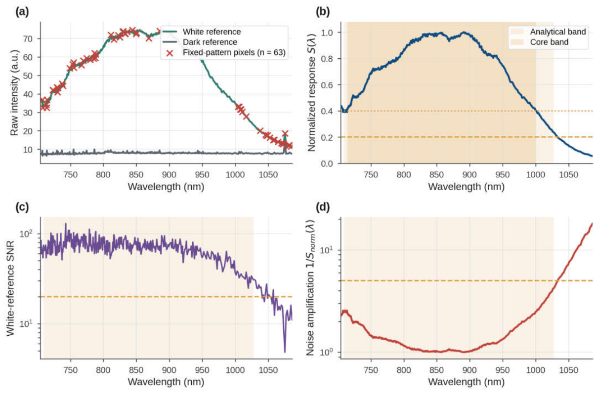
Figure 2.
Freeze-thaw effects on chevon spectra (n = 400 paired animals). (a) Mean absorbance ±1 SD. (b) Mean paired shift ΔA with its 95% CI and the share of animals with ΔA > 0. (c) Paired shift after SNV, with FDR-significant wavelengths shaded. (d) Between-animal SD, with Pitman-Morgan significant wavelengths shaded.
Figure 2.
Freeze-thaw effects on chevon spectra (n = 400 paired animals). (a) Mean absorbance ±1 SD. (b) Mean paired shift ΔA with its 95% CI and the share of animals with ΔA > 0. (c) Paired shift after SNV, with FDR-significant wavelengths shaded. (d) Between-animal SD, with Pitman-Morgan significant wavelengths shaded.
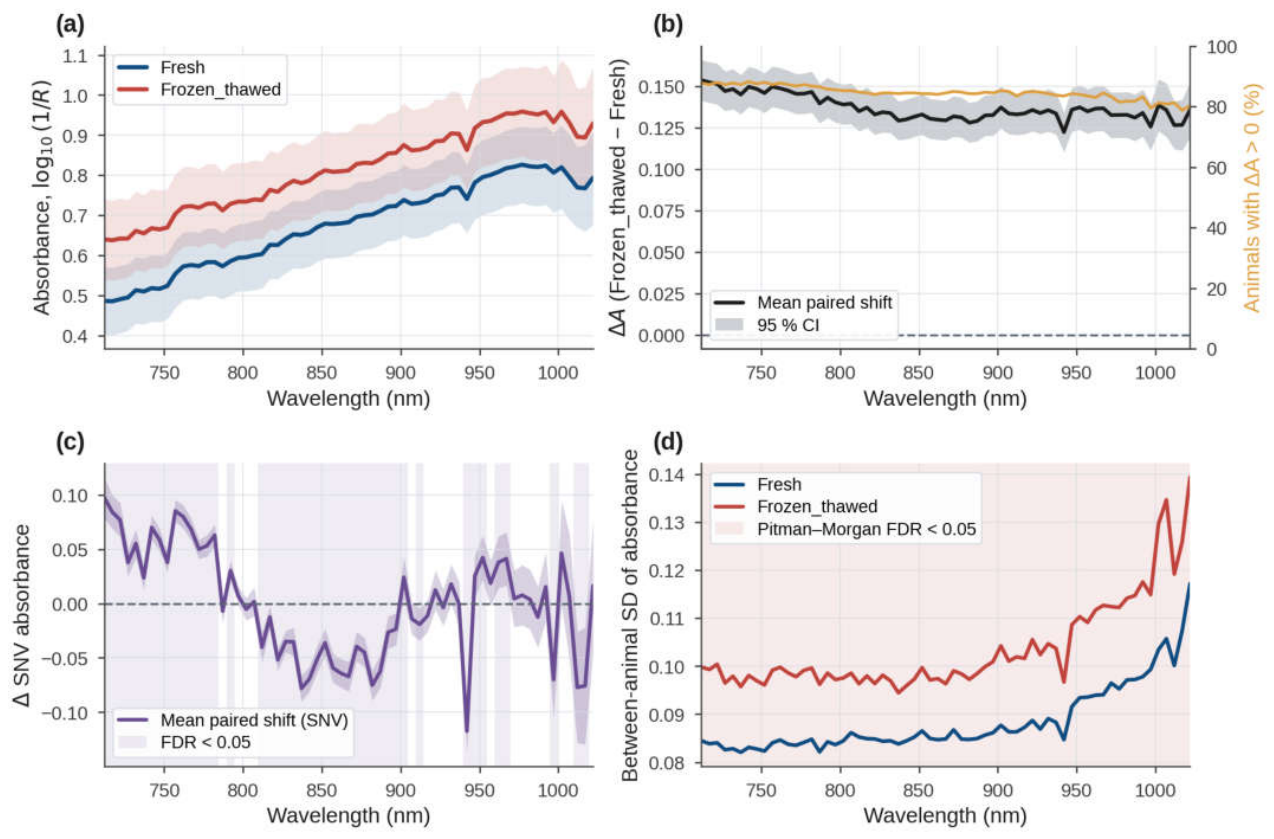
Figure 3.
PLS-DA on the training animals. (a) Latent-variable scores with 95% confidence ellipses. (b) Grouped-CV accuracy against the number of latent variables. (c) VIP scores and regression coefficients.
Figure 3.
PLS-DA on the training animals. (a) Latent-variable scores with 95% confidence ellipses. (b) Grouped-CV accuracy against the number of latent variables. (c) VIP scores and regression coefficients.
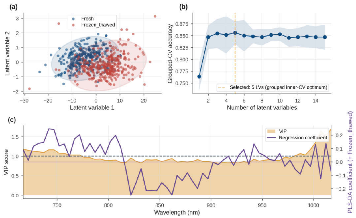
Figure 4.
Classification performance. (a) Nested-CV and independent test accuracy of all models. (b) Test-set ROC curves. (c) Test-set confusion matrix of the final SVM.
Figure 4.
Classification performance. (a) Nested-CV and independent test accuracy of all models. (b) Test-set ROC curves. (c) Test-set confusion matrix of the final SVM.
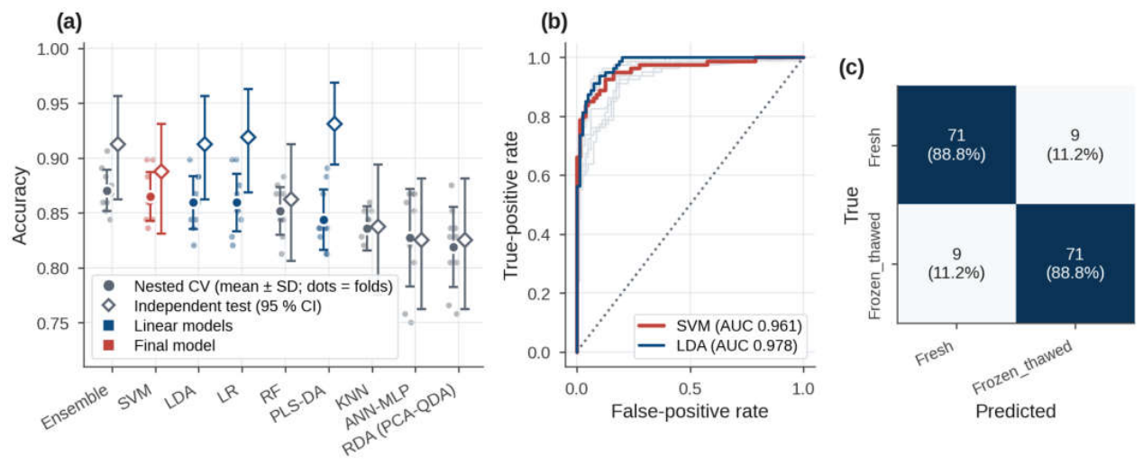
Figure 5.
Spectral regions and reduced models. (a) Class mean spectra with the consensus regions, where asterisks mark artifact-flagged regions. (b) Attribution profiles of the three method families and their consensus. (c) Accuracy of top-k and region-restricted models compared with random windows.
Figure 5.
Spectral regions and reduced models. (a) Class mean spectra with the consensus regions, where asterisks mark artifact-flagged regions. (b) Attribution profiles of the three method families and their consensus. (c) Accuracy of top-k and region-restricted models compared with random windows.
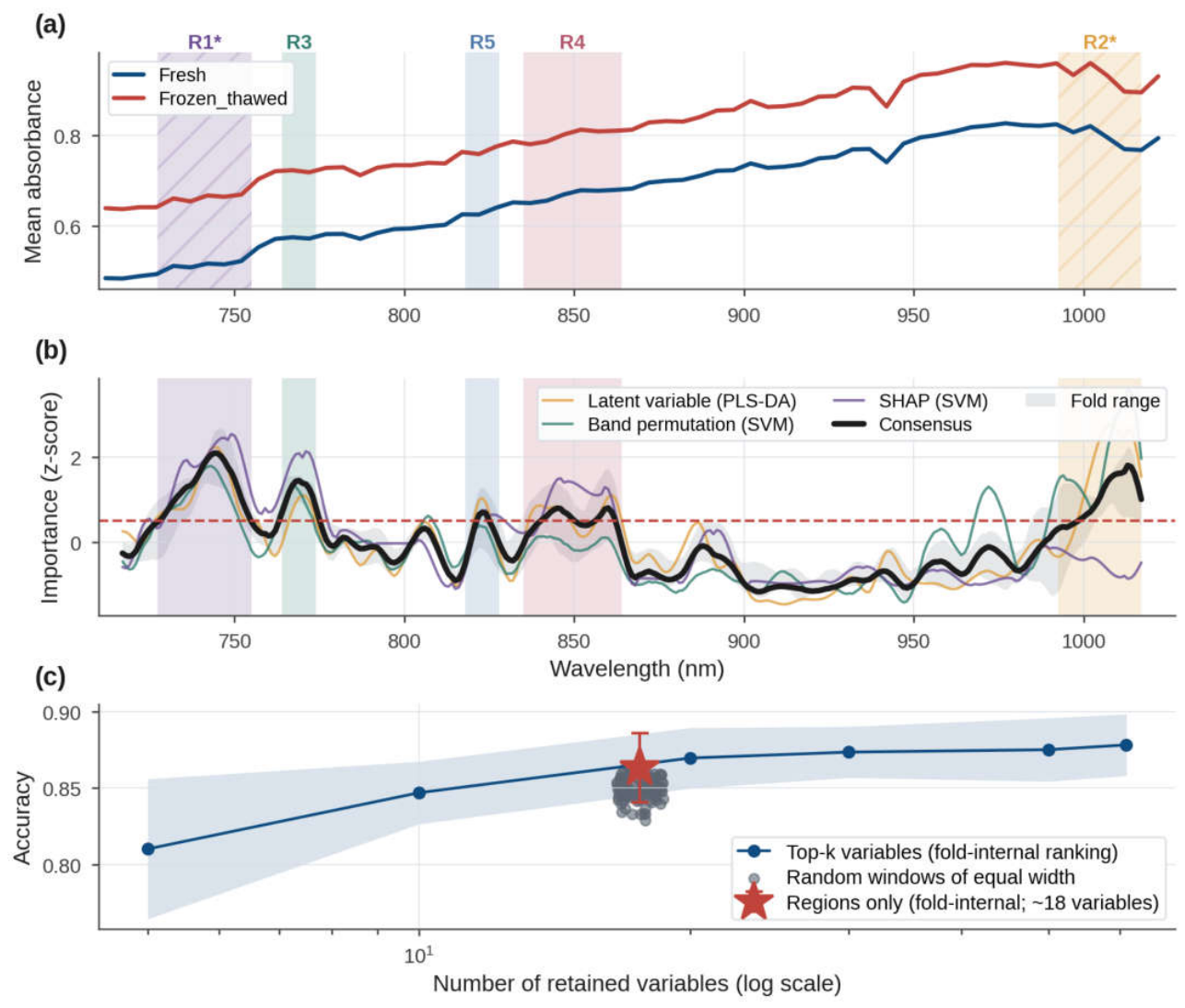

Table 1.
Nested animal-grouped cross-validated performance of the classifier panel on the training animals, with the optimal hyperparameters of the final models.
Table 1.
Nested animal-grouped cross-validated performance of the classifier panel on the training animals, with the optimal hyperparameters of the final models.
| Rank | Model | Hypothesis class | Optimal hyperparameters | Accuracy | Balanced accuracy | Sensitivity | Specificity | ROC-AUC | MCC | Fit time (s) | Prediction (ms/spectrum) |
| 1 | Ensemble (SVM + LDA + LR)a | Score ensemble | Members tuned individually | 0.870 ± 0.019 | 0.870 ± 0.019 | 0.880 ± 0.021 | 0.861 ± 0.028 | 0.929 ± 0.016 | 0.741 ± 0.038 | 0.64 | 0.170 |
| 2 | SVMb | Kernel | C = 10, γ = scale | 0.865 ± 0.022 | 0.865 ± 0.022 | 0.872 ± 0.034 | 0.858 ± 0.049 | 0.925 ± 0.020 | 0.732 ± 0.045 | 1.53 | 0.050 |
| 3 | LDA | Linear (shared covariance) | shrinkage = auto | 0.859 ± 0.024 | 0.859 ± 0.024 | 0.855 ± 0.026 | 0.864 ± 0.035 | 0.928 ± 0.016 | 0.719 ± 0.049 | 0.67 | 0.025 |
| 4 | LR | Linear (probabilistic) | C = 1 | 0.859 ± 0.026 | 0.859 ± 0.026 | 0.861 ± 0.030 | 0.858 ± 0.034 | 0.925 ± 0.015 | 0.719 ± 0.053 | 0.84 | 0.038 |
| 5 | RF | Ensemble (bagging) | max_features = 0.1 min_samples_leaf = 1 |
0.852 ± 0.022 | 0.852 ± 0.022 | 0.852 ± 0.036 | 0.852 ± 0.046 | 0.910 ± 0.015 | 0.705 ± 0.044 | 33.41 | 0.392 |
| 6 | PLS-DA | Linear (latent variable) | n_components = 5 | 0.844 ± 0.027 | 0.844 ± 0.027 | 0.834 ± 0.026 | 0.853 ± 0.044 | 0.921 ± 0.015 | 0.688 ± 0.055 | 1.59 | 0.022 |
| 7 | KNN | Distance-based | n_neighbors = 11 weights = distance |
0.836 ± 0.020 | 0.836 ± 0.020 | 0.831 ± 0.048 | 0.841 ± 0.043 | 0.889 ± 0.023 | 0.674 ± 0.041 | 0.65 | 0.076 |
| 8 | ANN-MLP | Neural network | alpha = 0.01 hidden_layer_sizes = (128, 64) |
0.827 ± 0.044 | 0.827 ± 0.044 | 0.816 ± 0.058 | 0.839 ± 0.059 | 0.897 ± 0.027 | 0.657 ± 0.088 | 2.10 | 0.034 |
| 9 | RDA (PCA-QDA) | Quadratic (class covariance) | n_components = 5 reg_param = 0.1 |
0.819 ± 0.036 | 0.819 ± 0.036 | 0.772 ± 0.066 | 0.866 ± 0.051 | 0.907 ± 0.022 | 0.643 ± 0.073 | 0.75 | 0.026 |
Values are mean ± SD across 10 outer folds (five-fold grouped CV repeated twice, with five-fold grouped inner tuning). Sensitivity denotes detection of frozen-thawed samples. Preprocessing used Savitzky–Golay smoothing (11 nm) and 5-nm binning over 710–1027 nm without scatter correction. Fit time includes inner tuning. The final model was selected as the simplest classifier within one SE (0.0060) of the highest nested-CV accuracy. Fully nested preprocessing yielded 0.860 ± 0.033 accuracy. Complete search spaces are provided in Table S5. ANN-MLP, multilayer perceptron; KNN, k-nearest neighbors; LDA, linear discriminant analysis; LR, logistic regression; MCC, Matthews correlation coefficient; PLS-DA, partial least squares discriminant analysis; RDA, regularized discriminant analysis; RF, random forest; ROC-AUC, area under the ROC curve; SVM, support vector machine. ᵃ Highest nested-CV accuracy. ᵇ Final selected model.
Table 2.
Performance on the independent animal-disjoint test set of all tuned classifiers, of the final model restricted to the consensus variables and of the shape-only and baseline-only models.
Table 2.
Performance on the independent animal-disjoint test set of all tuned classifiers, of the final model restricted to the consensus variables and of the shape-only and baseline-only models.
| Model | CV accuracy | Test accuracy | 95% CI | Sensitivity | Specificity | ROC-AUC | MCC | Prediction (ms/spectrum) | McNemar vs final (b/c, p) | Animal-level paired p |
| Tuned classifier panel | ||||||||||
| Ensemble (SVM + LDA + LR) | 0.870 | 0.913 | 0.863 to 0.956 | 0.925 | 0.900 | 0.972 | 0.825 | 0.080 | 0/4, 0.125 | 0.124 |
| SVM (final model) | 0.865 | 0.888 | 0.831 to 0.931 | 0.888 | 0.888 | 0.961 | 0.775 | 0.077 | NA | NA |
| LDA | 0.859 | 0.913 | 0.863 to 0.956 | 0.913 | 0.913 | 0.978 | 0.825 | 0.019 | 1/5, 0.219 | 0.217 |
| LR | 0.859 | 0.919 | 0.869 to 0.963 | 0.938 | 0.900 | 0.975 | 0.838 | 0.019 | 0/5, 0.062 | 0.064 |
| RF | 0.852 | 0.863 | 0.806 to 0.912 | 0.863 | 0.863 | 0.942 | 0.725 | 0.269 | 7/3, 0.344 | 0.403 |
| PLS-DA | 0.844 | 0.931 | 0.894 to 0.969 | 0.925 | 0.938 | 0.974 | 0.863 | 0.030 | 2/9, 0.065 | 0.091 |
| KNN | 0.836 | 0.838 | 0.775 to 0.894 | 0.850 | 0.825 | 0.922 | 0.675 | 0.042 | 10/2, 0.039 | 0.056 |
| ANN-MLP | 0.827 | 0.825 | 0.762 to 0.881 | 0.800 | 0.850 | 0.934 | 0.651 | 0.022 | 12/2, 0.013 | 0.014 |
| RDA (PCA-QDA) | 0.819 | 0.825 | 0.762 to 0.881 | 0.775 | 0.875 | 0.943 | 0.653 | 0.035 | 12/2, 0.013 | 0.006 |
| Reduced and diagnostic models | ||||||||||
| SVM, consensus regions only (20 variables) | 0.863 | 0.906 | 0.863 to 0.944 | 0.900 | 0.913 | 0.957 | 0.813 | 0.038 | 0/3, 0.250 | 0.246 |
| SVM, top-30 consensus variables | 0.873 | 0.919 | 0.875 to 0.956 | 0.913 | 0.925 | 0.962 | 0.838 | 0.035 | 0/5, 0.062 | 0.062 |
| SVM, shape only (SNV, broadband level removed) | 0.845 | 0.925 | 0.881 to 0.963 | 0.875 | 0.975 | 0.958 | 0.854 | NA | 7/13, 0.263 | 0.265 |
| LDA, baseline only (spectrum mean and SD, 2 variables) | 0.840 | 0.850 | 0.794 to 0.900 | 0.838 | 0.863 | 0.940 | 0.700 | NA | 10/4, 0.180 | 0.181 |
The test set included 80 independent animals (160 mean spectra), excluded from model development and selection. CV accuracy was estimated using grouped CV, with nested 10-fold CV for the panel and shape-only models. The 95% CI used 2,000 animal-level bootstrap resamples. Comparisons with the final SVM used exact McNemar tests (b/c, spectrum-level) and sign-flip permutation tests (animal-level). Shape-only and baseline models used SNV-transformed spectral shape and spectral mean/SD, respectively. NA, not applicable.
Table 3.
Class-conditional (Mondrian) split-conformal prediction with the final model on the independent test set.
Table 3.
Class-conditional (Mondrian) split-conformal prediction with the final model on the independent test set.
| Target confidence | Coverage (both classes) | Coverage Fresh | Coverage Frozen_thawed | Singleton sets (%) | Both-class sets (%) | Empty sets (%) | Accuracy of singletons | Mean set size |
| 80% | 0.863 | 0.850 | 0.875 | 95.0 | 0.0 | 5.0 | 0.908 | 0.95 |
| 90% | 0.956 | 0.988 | 0.925 | 83.8 | 16.2 | 0.0 | 0.948 | 1.16 |
| 95% | 0.994 | 1.000 | 0.988 | 56.2 | 43.8 | 0.0 | 0.989 | 1.44 |
Calibration used 160 spectra from 80 training animals, independent of model refitting. The final pipeline was refitted on the remaining 240 training animals and differs from the model in Table 2 (test accuracy = 0.894). Coverage represents the proportion of test spectra whose prediction sets contained the true class, with class-conditional guarantees at or above the target confidence. Singleton sets indicate definitive predictions, whereas both-class sets indicate samples requiring confirmatory analysis. Empty sets indicate no admissible class.
Disclaimer/Publisher’s Note: The statements, opinions and data contained in all publications are solely those of the individual author(s) and contributor(s) and not of MDPI and/or the editor(s). MDPI and/or the editor(s) disclaim responsibility for any injury to people or property resulting from any ideas, methods, instructions or products referred to in the content. |
© 2026 by the authors. Licensee MDPI, Basel, Switzerland. This article is an open access article distributed under the terms and conditions of the Creative Commons Attribution (CC BY) license (http://creativecommons.org/licenses/by/4.0/).
Copyright: This open access article is published under a Creative Commons CC BY 4.0 license, which permit the free download, distribution, and reuse, provided that the author and preprint are cited in any reuse.