

Submitted:
03 November 2026
Posted:
05 November 2026
You are already at the latest version
Abstract
Anticipating the heading rate and speed that a curve will demand is a key capability for automated driving. This study presents a multi-task convolutional neural network–long short-term memory (CNN-LSTM) model that predicts the change of the vehicle heading rate, used as a steering proxy, and of its speed over horizons of 1, 2, and 3 s from a 2 s window of features. The inputs combine a preview of the road geometry extracted from light detection and ranging (LiDAR) point clouds (the lateral offset of the road at 10–40 m ahead), road banking and grade, and the vehicle speed and heading rate. A one-sided physics-informed penalty discourages predicted speeds above the maximum cornering speed of a banked curve with friction. The model was trained on PandaSet and evaluated on held-out sequences over five random sequence-wise splits, and without retraining on three sequences of the KITTI raw dataset, against a persistence baseline and an ablation without the physics term. On unseen PandaSet sequences, the model reduced the speed mean squared error with respect to persistence by 15.7%, 23.0%, and 27.0% at 1, 2, and 3 s, and the heading-rate error by 3.7%–16.4%. On KITTI, heading-rate error was on par with persistence, whereas speed error was 24–43% higher. The physics term was never active, since all speeds were well below the physical limit. The code is openly available.
Keywords:
autonomous vehicles
; LiDAR
; CNN-LSTM
; physics-informed neural networks
; speed prediction
; heading rate prediction
; curved roads
1. Introduction
Curved road segments concentrate a large share of the difficulty of automated driving: the vehicle must anticipate how sharply to turn and how fast it can travel before it enters the curve, using only what its sensors perceive of the road ahead. Light detection and ranging (LiDAR) sensors provide dense three-dimensional measurements of the road surface and its surroundings [1], and public datasets such as PandaSet [2] make it possible to study these problems with real sensor data [3].
Autonomous Vehicles (AVs) are expected to improve road safety by mitigating human factors such as distraction and cognitive errors [4], and automated systems can anticipate hazardous situations through trajectory generation and prediction [5]. To do so, an AV must plan and execute maneuvers while accounting for road infrastructure, vehicle dynamics, and actuator constraints [6]. Road geometry is one of the most significant constraints in motion planning [7,8], and it becomes critical on curves, where the admissible speed depends on the curve radius, the banking of the road, and tire–road friction.
Two broad families of methods address this problem. Model-based approaches, such as Model Predictive Control (MPC), predict the vehicle response over a horizon and optimize steering and speed commands subject to explicit constraints [6,9]; they are interpretable but depend on accurate vehicle models. Learning-based approaches, from convolutional perception pipelines [10] to deep reinforcement learning [11,12], learn the mapping from sensor data to driving actions, but they offer no guarantee that their outputs respect physical limits. Physics-informed machine learning [13,14,15] offers a middle ground: physical knowledge is introduced into the training objective so that the learned model is discouraged from producing physically implausible outputs.
A useful predictor of future heading rate and speed must also be compared with an appropriate reference. Over short horizons, both signals change slowly, so simply repeating the last observed value (persistence) is already a strong predictor, and a learned model is only useful if it improves on it. The advantage that LiDAR can offer over persistence is anticipation: it perceives the geometry of the road ahead before the vehicle reaches it.
This work follows these ideas. A multi-task CNN-LSTM receives a 2 s window of features that include a preview of the road geometry extracted from LiDAR at several look-ahead distances, and it predicts the change of the heading rate, used as a steering proxy, and of the speed over horizons of 1, 2, and 3 s. A physics-informed term in the loss penalizes predicted speeds above the maximum cornering speed of a banked curve with friction. The main contributions are the following:
- A feature-extraction pipeline that derives the same road-geometry descriptors, including a look-ahead preview of the road, from the LiDAR point clouds of two datasets (PandaSet and KITTI), after transforming the PandaSet points from world coordinates to a vehicle-aligned frame.
- A multi-task CNN-LSTM that predicts changes with respect to the last observed values and is trained with a one-sided physics-informed loss based on the banked-curve speed limit.
- An evaluation over five sequence-wise splits and three prediction horizons that compares the model with a persistence baseline and with an ablation of the physics term, both on unseen PandaSet sequences and, without retraining, on KITTI [16], reporting where the model improves on the baseline and where it does not.
- An open implementation of the full pipeline to support reproducibility.
The remainder of the paper is organized as follows. Section 2 reviews related work. Section 3 describes the datasets, the physical background, the feature extraction, the model, and the evaluation protocol. Section 4 presents the results, Section 5 discusses them together with the limitations of the study, and Section 6 concludes the paper.
2. Related Work
Recent work on autonomous driving over curved paths has focused on curvature-aware planning and predictive tracking under dynamic and geometric constraints. Liu et al. [17] formulate a two-layer MPC architecture in which an outer layer generates a curvature-adaptive reference and an inner layer solves a constrained optimal control problem for path tracking, reducing lateral error at high speeds by incorporating curvature-dependent bounds on steering rate and lateral acceleration. Li et al. [18] perform trajectory planning directly in Cartesian coordinates instead of the Frenet frame, embedding vehicle kinematics and collision constraints in a nonlinear optimization that remains well posed on highly curved references. For large-curvature roads, Wang et al. [19] model the driver–vehicle–road interaction with a kinematic vehicle model coupled with an artificial potential field, producing smooth, collision-free trajectories when curvature varies abruptly. In unstructured environments, Min et al. [20] improve the A* algorithm by refining its heuristic, smoothing the resulting path, and incorporating vehicle contour and motion constraints. Yang et al. [21] augment a path-tracking controller with a prediction model of future lateral deviation, reducing steady-state error on curved segments.
Probabilistic models are also widely used to anticipate driver behavior: hidden Markov models have been applied to driver-intention prediction [22] and lane-change prediction [23], and Kalman filtering is a standard tool for estimating vehicle states from noisy measurements [24]. These methods model temporal dependencies explicitly but rely on hand-designed state representations.
On the learning side, physics-informed neural networks introduce governing equations into the loss function [14], and broader surveys describe how scientific knowledge can be integrated with machine learning through the architecture, the loss, or the data [13,15]. The present work combines these lines: it learns the mapping from LiDAR-derived geometry and vehicle dynamics to future heading rate and speed with a CNN-LSTM, and it constrains the predicted speed through a loss term derived from the banked-curve speed limit, without solving an optimization problem online.
3. Materials and Methods
Figure 1 summarizes the complete pipeline, from the raw sensor data to the evaluation. Each stage is described in the following subsections. All experiments were run on Google Colab [25] with an NVIDIA T4 GPU, using TensorFlow/Keras.
3.1. Datasets
PandaSet [2] contains more than 100 driving sequences of about 8 s each, recorded at 10 Hz with a 360° mechanical spinning LiDAR (Pandar64), a forward-facing LiDAR (PandarGT), six cameras, and GPS/IMU localization. In this work, the Pandar64 point clouds and the corresponding LiDAR sensor poses were used. A total of [XX] sequences with complete data and at least 51 frames were processed. Figure 2 shows a LiDAR frame of sequence 001.
KITTI raw [16] provides synchronized Velodyne HDL-64E point clouds and high-precision GPS/IMU (OXTS) measurements at 10 Hz. Three sequences of the Road category (2011_09_26, drives 0015, 0027, and 0028) were used exclusively for zero-shot evaluation; no KITTI data were used for training, validation, or fitting any preprocessing step.
3.2. Physical Background: Maximum Speed on a Banked Curve
For a vehicle of mass m moving along a curve of radius , the normal component of Newton’s second law gives
On a road banked by an angle and without friction, the vertical and normal force balances on the vehicle, with normal reaction N and weight , are
which yields the rated speed of the curve,
When tire–road friction with coefficient is included and the vehicle is at the limit of sliding outward, the maximum admissible speed becomes
Equation (4) is the physical constraint used in the loss function (Section 3.6). Note that the mass cancels out: the speed limit depends only on the curve radius, the banking angle, and friction. In this study, is fixed to a conservative value of 0.7, representative of dry pavement.
3.3. Feature Extraction
Eight features are computed for every frame: four road-preview offsets, the banking angle, the road grade, the vehicle speed v, and the heading rate . The turning radius R and the physical speed limit are also computed for the physics-informed loss but are not network inputs.
Coordinate frame. PandaSet stores its point clouds in world coordinates. This was verified by comparing, along sequence 001, the center of the point cloud with the sensor position: both moved by about 84 m between the first and last frames. Each frame is therefore transformed to a vehicle-aligned frame with its origin at the sensor, the x axis along the direction of travel, the y axis to the left, and the z axis kept as the world vertical, so that banking and grade are measured with respect to gravity. The yaw is estimated from the sensor trajectory as the direction of the displacement between frames and k; it is held constant when the displacement is below 0.05 m (vehicle practically stopped) and unwrapped to avoid jumps. KITTI Velodyne points are already expressed in the sensor frame with the same axis convention.
Road geometry from LiDAR. The same procedure is applied to both datasets. Points within 0–50 m ahead and m laterally are kept, and ground points are selected in a band from to m around the 10th percentile of their height. From these points:
- The road preview at distance m is the lateral position of the center of the ground extent in a 5 m slice centered at d, computed as the midpoint of the 10th and 90th percentiles of y. As the road bends, these offsets shift toward the inside of the curve, increasingly with distance.
- The grade is (%), using ground points beyond 40 m and within 10 m.
- The banking angle iswhere the subscripts r and l denote the ground points within 20 m to the right and left of their median lateral position.
Missing values (for example, a slice with too few ground points) are filled with the previous valid value. Figure 3 illustrates the ground points and the road boundaries in the vehicle frame.
Vehicle dynamics. In PandaSet, the speed is computed from the three-dimensional displacement between consecutive sensor poses, (km/h) with s, and the heading rate is the frame-to-frame difference of the yaw smoothed with a trailing three-frame moving average (only past frames are used). Figure 4 shows the speed profile of sequence 001. In KITTI, the speed is the OXTS forward velocity and the heading rate is computed in the same way from the unwrapped OXTS yaw. The turning radius follows from circular-motion kinematics, with and Hz, clipped to 5–1000 m, and is obtained from Eq. (4) with R and .
3.4. Sequence Construction
The per-frame features are converted into supervised samples with a sliding window. Each input contains the eight features of 20 consecutive frames (2.0 s of history). For a horizon of frames (1, 2, and 3 s), the targets are the mean heading rate (deg/frame) and the mean speed (km/h) over the following H frames. The network does not predict these values directly but their change with respect to the last observed frame of the window, and ; the final prediction is the last observed value plus the predicted change. A predicted change of zero corresponds to the persistence baseline. For the physics term, the most restrictive limit within the horizon, , is stored with each sample.
3.5. CNN-LSTM Architecture
The network (Table 1) combines one-dimensional convolutions along the time axis, which extract local temporal patterns from the input window, with an LSTM layer, which models longer temporal dependencies. Causal padding ensures that each convolutional output depends only on current and past frames. Dropout is used to limit overfitting, and two linear output heads predict the heading-rate and speed changes.
3.6. Physics-Informed Loss
The physics term is a one-sided (hinge) penalty that is zero whenever the predicted speed is below the physical limit:
and the total loss is
with m/s2 and in Eq. (4) (the denominator is bounded below by 0.05 to avoid numerical blow-up). The penalty is computed in the standardized space of the speed change: the limit is standardized with the same scaler as and supplied through an auxiliary input that bypasses the CNN-LSTM backbone. The constraint therefore acts on the gradients during training and is not a network input. Because it involves only the speed output, it is not expected to affect the heading-rate prediction directly.
3.7. Training and Evaluation Protocol
Figure 5 summarizes the evaluation protocol. The PandaSet sequences were split at random, by whole sequences, into training (about 68%), validation (about 12%), and test (20%) sets, so that windows of the same sequence never appear in more than one set. Inputs and targets were standardized with scalers fitted on the training sequences only, and the same scalers were applied, without refitting, to the validation and test sequences and to KITTI. Early stopping on the validation loss selected the weights of each model. To assess the sensitivity of the results to the choice of test sequences, the entire procedure was repeated for five different random splits, and results are reported as the mean and standard deviation over the splits.
Three predictors were compared:
- Persistence baseline: predicts that the mean heading rate and speed over the horizon equal their last observed values. It requires no training.
- CNN-LSTM without PIDL: the architecture of Table 1 trained with (ablation).
- CNN-LSTM with PIDL: the proposed model ().
Performance is reported with the mean squared error (MSE) and the coefficient of determination () of each output in its original units. Because all predictors are evaluated on the same samples within each split, the main comparison is the relative change of MSE with respect to persistence, computed per split and then averaged, together with the number of splits in which the network obtains a lower MSE. The percentage of predicted speeds above is also reported.
4. Results
Each test split contained 8 PandaSet sequences (408, 328, and 248 samples at horizons of 1, 2, and 3 s), and the three KITTI sequences provided 828, 798, and 768 samples. Unless otherwise stated, values are the mean ± standard deviation over the five splits.
4.1. Training Behavior
Figure 6 shows the training and validation loss of the proposed model in the first split at the 1 s horizon. The validation loss reached its minimum after four epochs and increased afterwards, while the training loss continued to decrease; early stopping retained the weights of the best validation epoch, which prevents the overfitting observed when training for a fixed number of epochs.
4.2. Comparison with the Persistence Baseline
Table 2 reports the MSE of the persistence baseline and of the proposed model, together with the relative change of MSE and the number of splits in which the model was better; Figure 7 shows the relative changes graphically.
On unseen PandaSet sequences, the model reduced the speed MSE with respect to persistence by 15.7% at 1 s (lower error in 4 of 5 splits), 23.0% at 2 s, and 27.0% at 3 s (5 of 5 splits in both cases). The heading-rate MSE decreased by 3.7% at 1 s (5 of 5 splits), 16.4% at 2 s (4 of 5), and 13.7% at 3 s (3 of 5), with a large variability across splits at the longer horizons.
On KITTI, without retraining, the heading-rate MSE was on par with persistence at all horizons (relative changes between and ). The speed MSE, in contrast, was higher than that of persistence by 24.4%, 40.8%, and 42.9% at 1, 2, and 3 s, and the model was better in at most one of the five splits.
4.3. Coefficient of Determination
Table 3 reports for completeness. The speed is high for all predictors because the speed varies little within a few seconds. The heading-rate on PandaSet varies strongly between splits (standard deviation of about 0.6–0.85) and is negative at the longer horizons for both predictors: the test sequences of some splits contain mostly straight driving, where the variance of the heading rate is very small and becomes unstable. For this reason, the relative MSE comparison of Table 2 is used as the main criterion.
4.4. Ablation of the Physics Term
In all 30 runs (five splits and three horizons), the CNN-LSTM trained with and without the physics term produced identical metrics to four decimal places, and no predicted speed exceeded in either configuration. The physics penalty was therefore never active during training: all target and predicted speeds were well below the cornering limit given by Eq. (4) with .
5. Discussion
Within PandaSet, the CNN-LSTM consistently predicted speed better than persistence, and the advantage grew with the horizon, from 15.7% at 1 s to 27.0% at 3 s. This pattern is consistent with the role of the road-geometry preview: over one second, the future speed is close to the current one and there is little to gain, whereas over two or three seconds the geometry ahead provides information about upcoming decelerations and accelerations that the last observed value cannot contain. The heading-rate error also decreased with respect to persistence, but less consistently across splits; the heading rate is a noisier target, and the preview features are a coarse description of the road, based on the extent of the ground points rather than on detected lane markings.
The zero-shot results on KITTI show the limits of this generalization. Even though the road-geometry features are now computed with the same procedure from the LiDAR of both datasets, the model did not improve on persistence: the heading-rate error was on par with it, and the speed error was clearly higher. A plausible explanation is a shift in the speed distribution: the KITTI sequences reach speeds close to 80 km/h, whereas the PandaSet training data are mostly below 50 km/h, so the speed changes learned on PandaSet do not extrapolate well. The two datasets also differ in LiDAR sensor, mounting height, and driving environment, which affect the ground filtering and the preview offsets. Training on more diverse data, or adapting the model to the target domain, would be required to obtain a benefit over persistence in a new dataset.
The physics-informed term did not influence the results. In the tested data, the predicted speeds never approached the physical cornering limit, so the one-sided penalty remained zero and did not contribute to the gradients. In this setting, the term acts only as a safeguard that would become active if the network predicted physically inadmissible speeds; its effect on accuracy can only be evaluated on data that include speeds close to the limit, such as sharper curves, higher speeds, or lower friction.
Table 4 places the proposed approach qualitatively next to representative methods from the literature. Each method was evaluated with its own data and conditions, so the comparison describes the characteristics of each approach rather than a benchmark on common data.
5.1. Limitations
Several limitations should be considered when interpreting these results:
- Size of the evaluation. Each test split contains only eight PandaSet sequences, and the zero-shot evaluation uses three KITTI sequences. The variability across splits is large for the heading rate, and more data would be needed to establish the size of the improvements more precisely.
- Physics term. The physics-informed penalty was never active in the tested data, so its effect on accuracy could not be assessed.
- Cross-dataset generalization. The model did not improve on persistence when applied to KITTI without retraining, and its speed error was higher than that of persistence.
- Road preview. The preview offsets are derived from the extent of the ground points, without lane or road-boundary detection, and can be affected by sidewalks, parked vehicles, or open areas next to the road.
- Steering proxy. The heading rate of the vehicle is used as a proxy for steering; the steering-wheel angle itself is not available in the datasets used.
- Physical model. The friction coefficient is fixed at 0.7 rather than estimated, and only the lateral cornering limit is modeled, not the combined longitudinal and lateral friction ellipse.
- Offline validation. All experiments are offline. Closed-loop control, hardware-in-the-loop testing, actuator delays, and deployment on a vehicle were not evaluated.
6. Conclusions
This study presented a multi-task CNN-LSTM that predicts the heading rate and speed of a vehicle over horizons of 1 to 3 s from a LiDAR-based preview of the road geometry and the recent vehicle dynamics, trained with a physics-informed loss based on the maximum cornering speed of a banked curve with friction, and evaluated against a persistence baseline over five sequence-wise splits. On unseen PandaSet sequences, the model reduced the speed error with respect to persistence by 15.7% to 27.0%, with an advantage that grew with the horizon, and the heading-rate error by 3.7% to 16.4%. Without retraining, it did not improve on persistence on KITTI, where its speed error was higher. The physics-informed term was never active because all speeds remained well below the physical limit.
These results indicate that a LiDAR preview of the road geometry contains useful information to anticipate speed changes beyond a simple persistence model within the same domain, but that this benefit does not transfer directly to a different dataset. They also show the importance of comparing learned predictors with simple baselines and across several data splits.
Future work will focus on (i) training on larger and more diverse datasets and evaluating domain adaptation, (ii) improving the road preview with lane and road-boundary detection, (iii) evaluating the physics-informed term on data closer to the physical limits and with a dynamically estimated friction coefficient, (iv) incorporating the steering-wheel angle where available, and (v) validating the system in closed loop and on an instrumented vehicle, including deployment on embedded hardware such as the NVIDIA Jetson platform. In the long term, this line of work aims to contribute to advanced driver assistance systems for curve negotiation, in line with the goals of the Latin New Car Assessment Programme (Latin NCAP) of promoting active safety technologies in the region.
Author Contributions
Conceptualization, L.M.Z.A. and H.G.R.; methodology, L.M.Z.A. and H.G.R.; software, L.M.Z.A.; validation, L.M.Z.A., H.G.R. and J.I.D.l.R.V.; formal analysis, L.M.Z.A. and J.I.D.l.R.V.; investigation, L.M.Z.A.; resources, H.G.R.; data curation, L.M.Z.A.; writing—original draft preparation, L.M.Z.A.; writing—review and editing, H.G.R. and J.I.D.l.R.V.; visualization, L.M.Z.A.; supervision, H.G.R. and J.I.D.l.R.V.; project administration, H.G.R.; funding acquisition, L.M.Z.A. All authors have read and agreed to the published version of the manuscript.
Funding
This research was funded by the Secretaría de Ciencia, Humanidades, Tecnología e Innovación (SECIHTI), Mexico, through a postgraduate scholarship, grant number 2022-000018-02NACF.
Institutional Review Board Statement
Not applicable.
Informed Consent Statement
Not applicable.
Data Availability Statement
The data analyzed in this study are openly available from public repositories. PandaSet is available at https://scale.com/open-datasets/pandaset, and the KITTI raw dataset is available at https://www.cvlibs.net/datasets/kitti/raw_data.php. The source code used to process the data, train the models, and generate the figures is available at https://github.com/DrLuisZapata/lidar-cnn-lstm-curves.
Acknowledgments
During the preparation of this manuscript, the authors used Claude (Anthropic) [26] for generating the diagrams in Figure 1 and Figure 5 and plotting Figure 7 from the computed results. All experiments were run by the authors, and all reported results were computed by the published code from the original data. The authors have reviewed and edited the output and take full responsibility for the content of this publication.
Conflicts of Interest
The authors declare no conflicts of interest. The funders had no role in the design of the study; in the collection, analyses, or interpretation of data; in the writing of the manuscript; or in the decision to publish the results.
Abbreviations
The following abbreviations are used in this manuscript:
| AV | Autonomous Vehicle |
| CNN | Convolutional Neural Network |
| DRL | Deep Reinforcement Learning |
| GPS | Global Positioning System |
| IMU | Inertial Measurement Unit |
| LiDAR | Light Detection and Ranging |
| LSTM | Long Short-Term Memory |
| MPC | Model Predictive Control |
| MSE | Mean Squared Error |
| NCAP | New Car Assessment Programme |
| OXTS | Oxford Technical Solutions (GPS/IMU unit used in KITTI) |
| PIDL | Physics-Informed Deep Learning |
| ReLU | Rectified Linear Unit |
References
- Liang, D.; Zhang, C.; Zhang, P.; et al. Evolution of laser technology for automotive LiDAR, an industrial viewpoint. Nat. Commun. 2024, 15, 7660. [Google Scholar] [CrossRef]
- Xiao, P.; Shao, Z.; Hao, S.; Zhang, Z.; Chai, X.; Jiao, J.; Li, Z.; Wu, J.; Sun, K.; Jiang, K.; Wang, Y.; Yang, D. PandaSet: Advanced sensor suite dataset for autonomous driving. In Proceedings of the 2021 IEEE International Intelligent Transportation Systems Conference (ITSC), Indianapolis, IN, USA, 19–22 September 2021; pp. 3095–3101. [Google Scholar] [CrossRef]
- Liu, M.; Yurtsever, E.; Fossaert, J.; Zhou, X.; Zimmer, W.; Cui, Y.; Zagar, B.L.; Knoll, A.C. A survey on autonomous driving datasets: Statistics, annotation quality, and a future outlook. IEEE Trans. Intell. Veh. 2024, 9, 7138–7164. [Google Scholar] [CrossRef]
- Celaya-Padilla, J.M.; Galván-Tejada, C.E.; Lozano-Aguilar, J.S.A.; Zanella-Calzada, L.A.; Luna-García, H.; Galván-Tejada, J.I.; Gamboa-Rosales, N.K.; Rodriguez, A.V.; Gamboa-Rosales, H. Texting & driving detection using deep convolutional neural networks. Appl. Sci. 2019, 9, 2962. [Google Scholar] [CrossRef]
- Rastelli, J.P.; Lattarulo, R.; Nashashibi, F. Dynamic trajectory generation using continuous-curvature algorithms for door to door assistance vehicles. In Proceedings of the 2014 IEEE Intelligent Vehicles Symposium (IV), Dearborn, MI, USA, 8–11 June 2014; pp. 510–515. [Google Scholar] [CrossRef]
- Rasekhipour, Y.; Khajepour, A.; Chen, S.-K.; Litkouhi, B. A potential field-based model predictive path-planning controller for autonomous road vehicles. IEEE Trans. Intell. Transp. Syst. 2017, 18, 1255–1267. [Google Scholar] [CrossRef]
- Kim, B.; Yi, K. Probabilistic and holistic prediction of vehicle states using sensor fusion for application to integrated vehicle safety systems. IEEE Trans. Intell. Transp. Syst. 2014, 15, 2178–2190. [Google Scholar] [CrossRef]
- González, D.; Pérez, J.; Milanés, V.; Nashashibi, F. A review of motion planning techniques for automated vehicles. IEEE Trans. Intell. Transp. Syst. 2016, 17, 1135–1145. [Google Scholar] [CrossRef]
- Farag, W. Complex-track following in real-time using model-based predictive control. Int. J. Intell. Transp. Syst. Res. 2021, 19, 112–127. [Google Scholar] [CrossRef]
- Padmaja, B.; Rao, P.V.N.; Bala, M.M.; Patro, E.K.R. A novel design of autonomous cars using IoT and visual features. In Proceedings of the 2nd International Conference on I-SMAC (IoT in Social, Mobile, Analytics and Cloud), Palladam, India, 30–31 August 2018; pp. 18–21. [Google Scholar] [CrossRef]
- Kendall, A.; Hawke, J.; Janz, D.; Mazur, P.; Reda, D.; Allen, J.-M.; Lam, V.-D.; Bewley, A.; Shah, A. Learning to drive in a day. In Proceedings of the 2019 International Conference on Robotics and Automation (ICRA), Montreal, QC, Canada, 20–24 May 2019; pp. 8248–8254. [Google Scholar] [CrossRef]
- Sallab, A.E.; Abdou, M.; Perot, E.; Yogamani, S. Deep reinforcement learning framework for autonomous driving. Electron. Imaging 2017, 2017, 70–76. [Google Scholar] [CrossRef]
- Karniadakis, G.E.; Kevrekidis, I.G.; Lu, L.; Perdikaris, P.; Wang, S.; Yang, L. Physics-informed machine learning. Nat. Rev. Phys. 2021, 3, 422–440. [Google Scholar] [CrossRef]
- Raissi, M.; Perdikaris, P.; Karniadakis, G.E. Physics-informed neural networks: A deep learning framework for solving forward and inverse problems involving nonlinear partial differential equations. J. Comput. Phys. 2019, 378, 686–707. [Google Scholar] [CrossRef]
- Willard, J.; Jia, X.; Xu, S.; Steinbach, M.; Kumar, V. Integrating scientific knowledge with machine learning for engineering and environmental systems. ACM Comput. Surv. 2023, 55, 66. [Google Scholar] [CrossRef]
- Geiger, A.; Lenz, P.; Stiller, C.; Urtasun, R. Vision meets robotics: The KITTI dataset. Int. J. Robot. Res. 2013, 32, 1231–1237. [Google Scholar] [CrossRef]
- Liu, H.; Sun, J.; Cheng, K.W.E. A two-layer model predictive path-tracking control with curvature adaptive method for high-speed autonomous driving. IEEE Access 2023, 11, 89228–89239. [Google Scholar] [CrossRef]
- Li, B.; Ouyang, Y.; Li, L.; Zhang, Y. Autonomous driving on curvy roads without reliance on Frenet frame: A Cartesian-based trajectory planning method. IEEE Trans. Intell. Transp. Syst. 2022, 23, 15729–15741. [Google Scholar] [CrossRef]
- Wang, J.; Yan, Y.; Zhang, K.; Chen, Y.; Cao, M.; Yin, G. Path planning on large curvature roads using driver-vehicle-road system based on the kinematic vehicle model. IEEE Trans. Veh. Technol. 2022, 71, 311–325. [Google Scholar] [CrossRef]
- Min, H.; Xiong, X.; Wang, P.; Yu, Y. Autonomous driving path planning algorithm based on improved A* algorithm in unstructured environment. Proc. Inst. Mech. Eng. Part D. J. Automob. Eng. 2021, 235, 513–526. [Google Scholar] [CrossRef]
- Yang, J.; Bao, H.; Ma, N.; Xuan, Z. An algorithm of curved path tracking with prediction model for autonomous vehicle. In Proceedings of the 13th International Conference on Computational Intelligence and Security (CIS), Hong Kong, China, 15–18 December 2017; pp. 405–408. [Google Scholar] [CrossRef]
- Tran, D.; Sheng, W.; Liu, L.; Liu, M. A hidden Markov model based driver intention prediction system. In Proceedings of the IEEE International Conference on Cyber Technology in Automation, Control, and Intelligent Systems (CYBER), Shenyang, China, 8–12 June 2015; pp. 115–120. [Google Scholar] [CrossRef]
- Yuan, W.; Li, Z.; Wang, C. Lane-change prediction method for adaptive cruise control system with hidden Markov model. Adv. Mech. Eng. 2018, 10. [Google Scholar] [CrossRef]
- Olivera, R.; Olivera, R.; Vite, O.; Gamboa, H.; Navarrete, M.A.; Rivera, C.A. Application of the three state Kalman filtering for moving vehicle tracking. IEEE Lat. Am. Trans. 2016, 14, 2072–2076. [Google Scholar] [CrossRef]
- Google. Google Colaboratory. Available online: https://colab.research.google.com (accessed on 11 September 2026).
- Anthropic. Claude (claude-sonnet-4-6). Available online: https://claude.ai (accessed on 11 September 2026).
Figure 1.
Overview of the proposed method: per-frame feature extraction from PandaSet and KITTI, construction of sliding-window sequences, the multi-task CNN-LSTM with the physics-informed loss, training over five sequence-wise splits, and evaluation. The diagram was rendered with the assistance of an AI tool [26]; its content reflects the implementation described in this section.
Figure 1.
Overview of the proposed method: per-frame feature extraction from PandaSet and KITTI, construction of sliding-window sequences, the multi-task CNN-LSTM with the physics-informed loss, training over five sequence-wise splits, and evaluation. The diagram was rendered with the assistance of an AI tool [26]; its content reflects the implementation described in this section.
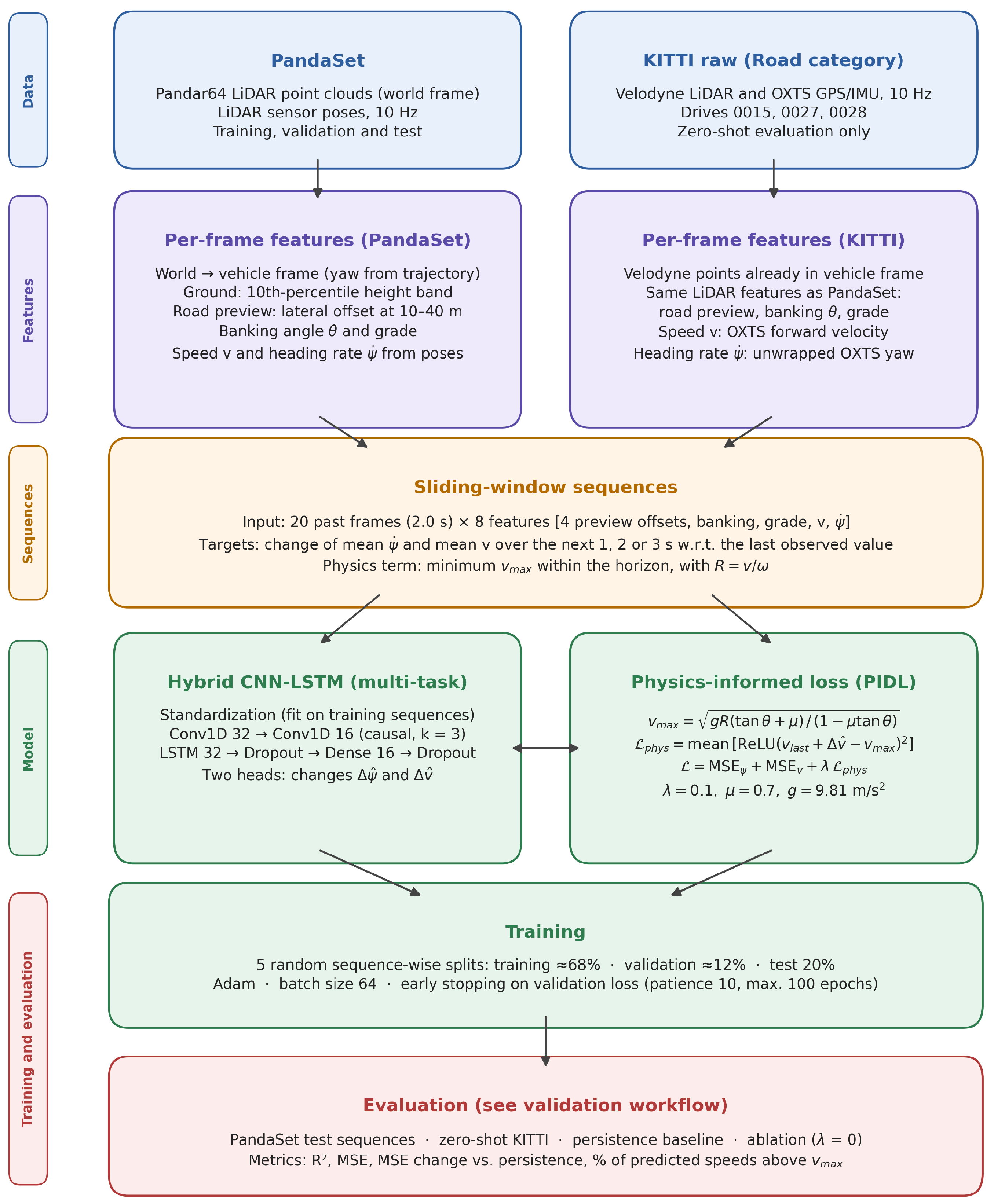
Figure 2.
LiDAR point cloud of PandaSet sequence 001, frame 00, in the vehicle-aligned frame and colored by height.
Figure 2.
LiDAR point cloud of PandaSet sequence 001, frame 00, in the vehicle-aligned frame and colored by height.
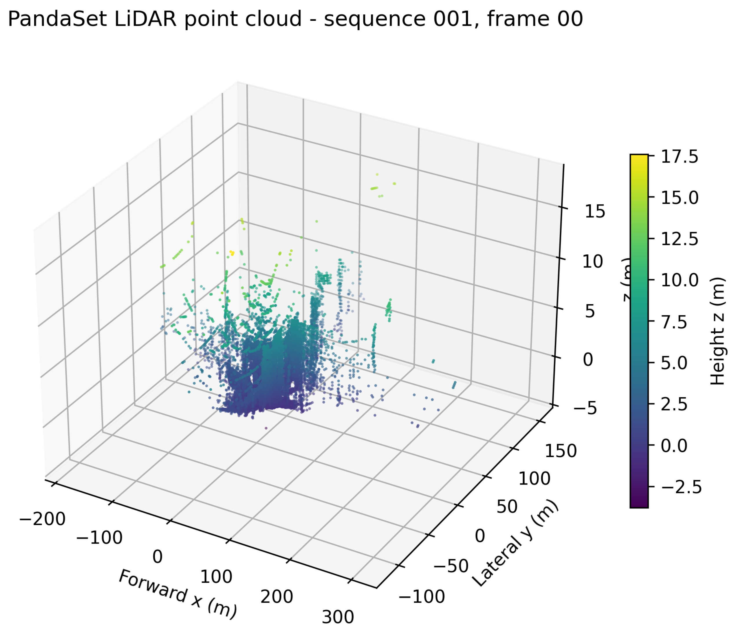
Figure 3.
Bird’s-eye view of the ground points of PandaSet sequence 001, frame 00, in the vehicle-aligned frame, split into left and right road boundaries, with the estimated road centerline and the ego vehicle at the origin.
Figure 3.
Bird’s-eye view of the ground points of PandaSet sequence 001, frame 00, in the vehicle-aligned frame, split into left and right road boundaries, with the estimated road centerline and the ego vehicle at the origin.
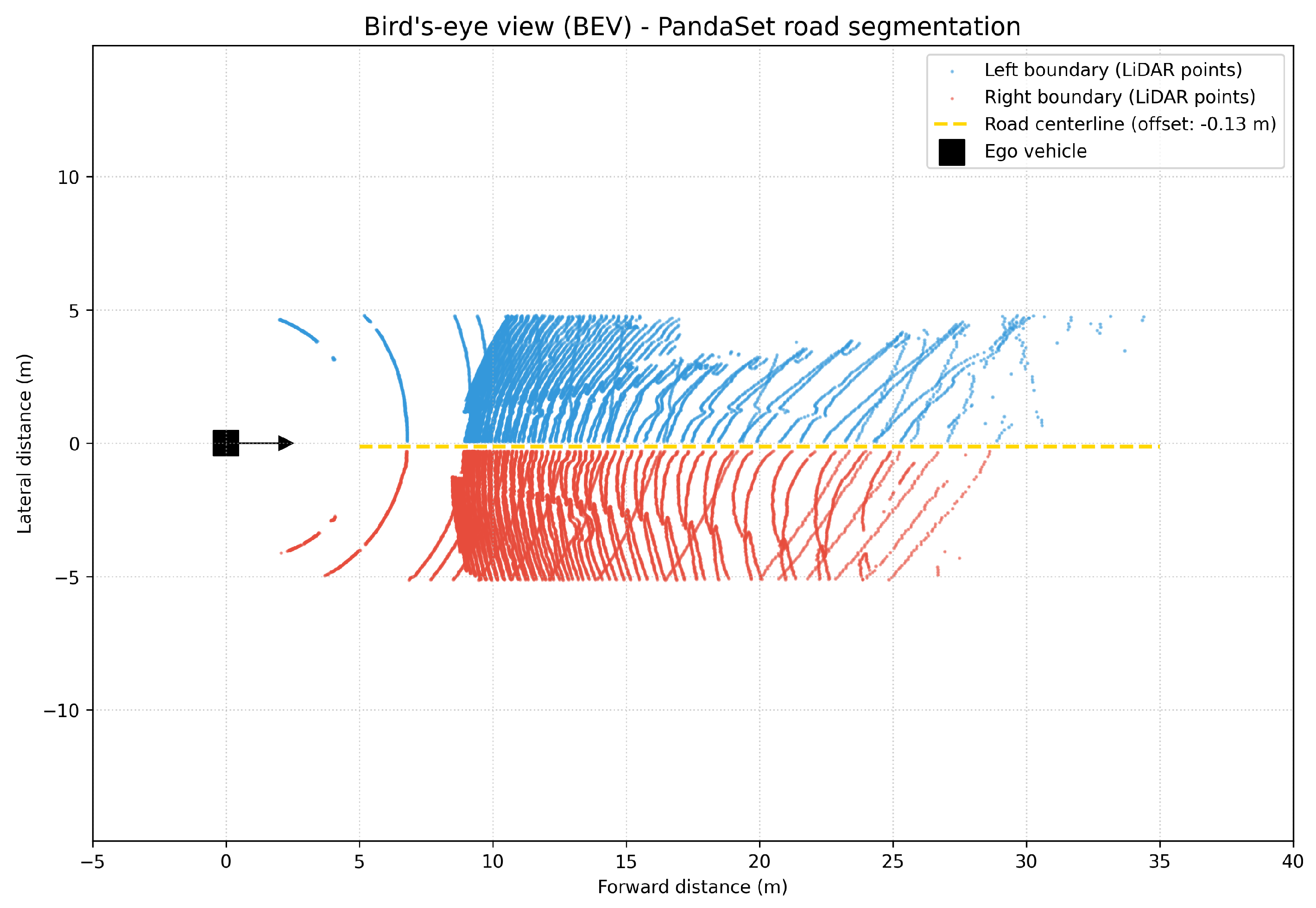
Figure 4.
Vehicle speed computed from the LiDAR sensor poses along PandaSet sequence 001.
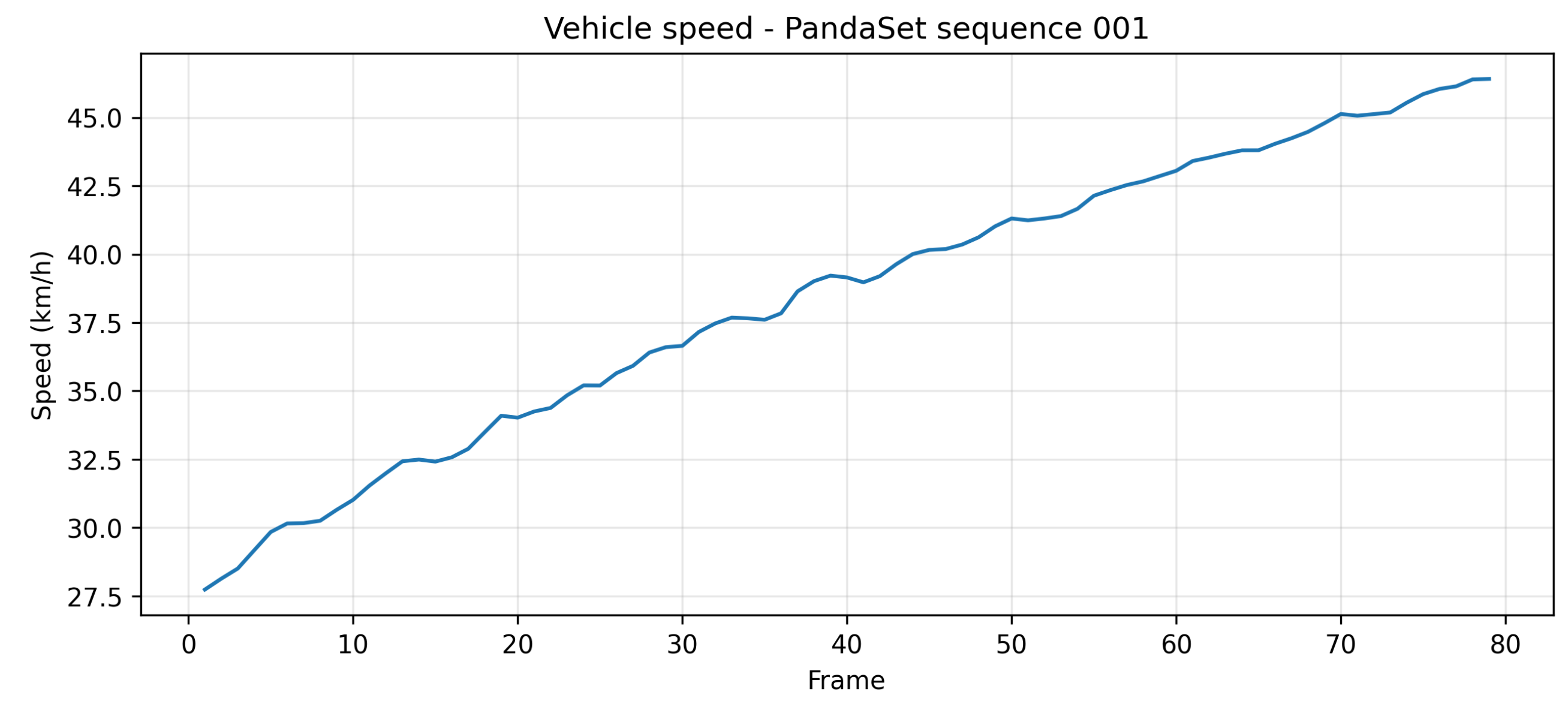
Figure 5.
Evaluation protocol: in-domain evaluation on unseen PandaSet test sequences and zero-shot evaluation on KITTI Road for three predictors, repeated over five random sequence-wise splits. The diagram was rendered with the assistance of an AI tool [26].
Figure 5.
Evaluation protocol: in-domain evaluation on unseen PandaSet test sequences and zero-shot evaluation on KITTI Road for three predictors, repeated over five random sequence-wise splits. The diagram was rendered with the assistance of an AI tool [26].
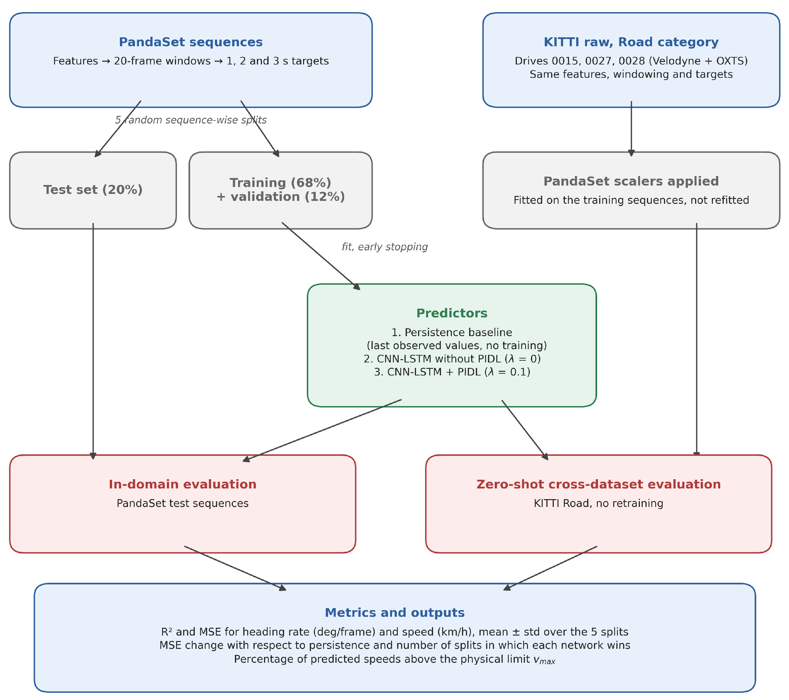
Figure 6.
Training and validation loss of the CNN-LSTM with the physics-informed term (first split, 1 s horizon). The dotted line marks the epoch selected by early stopping.
Figure 6.
Training and validation loss of the CNN-LSTM with the physics-informed term (first split, 1 s horizon). The dotted line marks the epoch selected by early stopping.
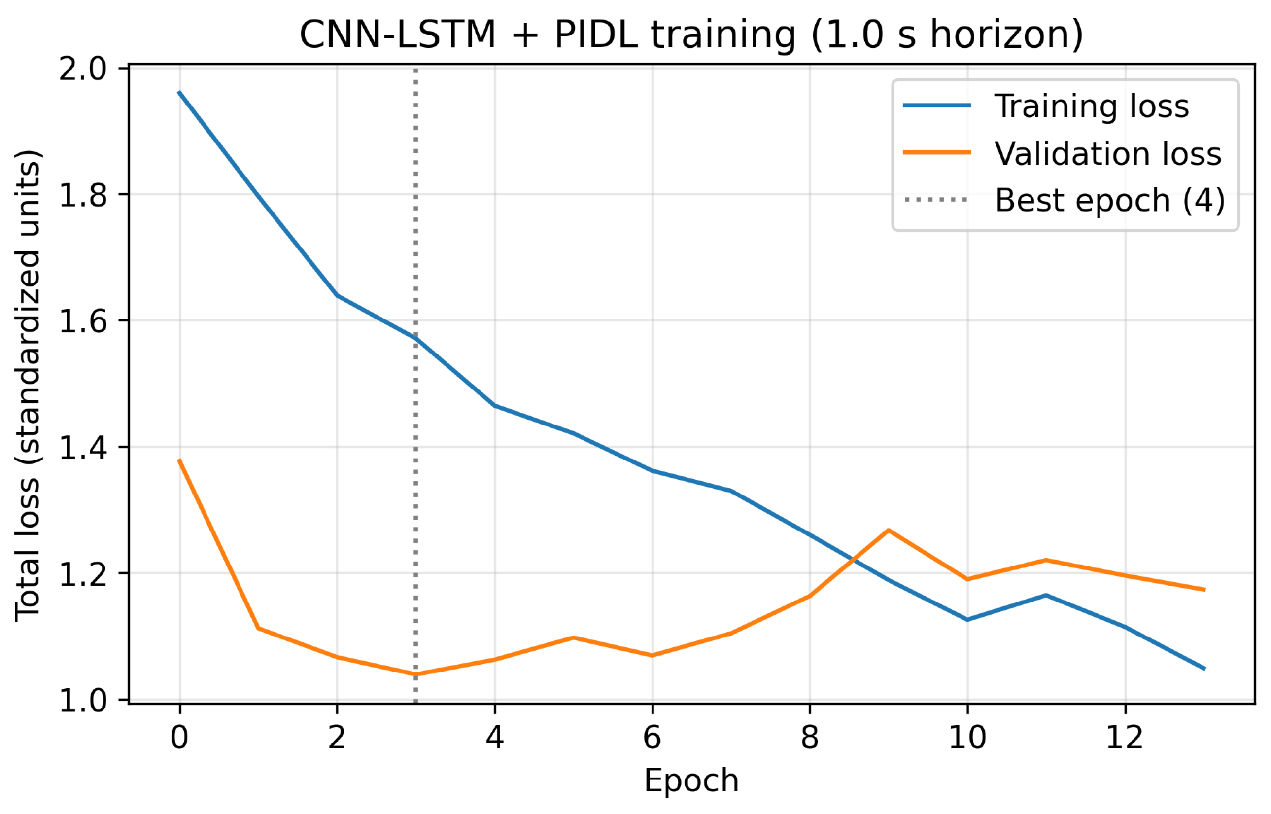
Figure 7.
Relative change of MSE of the CNN-LSTM with the physics term with respect to the persistence baseline (mean ± standard deviation over five splits) for heading rate (left) and speed (right). Negative values indicate a lower error than persistence; labels show the number of splits in which the model obtained a lower MSE.
Figure 7.
Relative change of MSE of the CNN-LSTM with the physics term with respect to the persistence baseline (mean ± standard deviation over five splits) for heading rate (left) and speed (right). Negative values indicate a lower error than persistence; labels show the number of splits in which the model obtained a lower MSE.
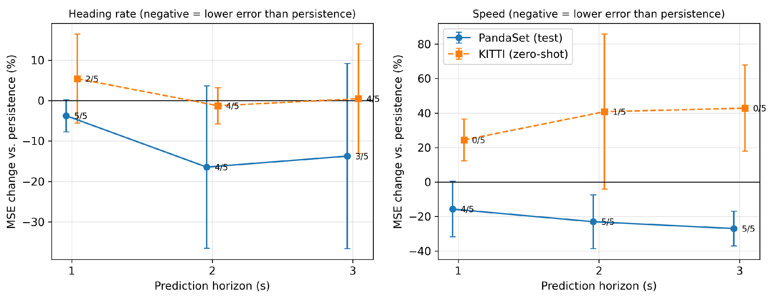
Figure 8.
Predicted versus actual heading rate and speed of the CNN-LSTM with the physics term on the PandaSet test sequences (top) and on KITTI Road without retraining (bottom), first split, 1 s horizon. The dashed line indicates perfect prediction. The values correspond to this split only.
Figure 8.
Predicted versus actual heading rate and speed of the CNN-LSTM with the physics term on the PandaSet test sequences (top) and on KITTI Road without retraining (bottom), first split, 1 s horizon. The dashed line indicates perfect prediction. The values correspond to this split only.
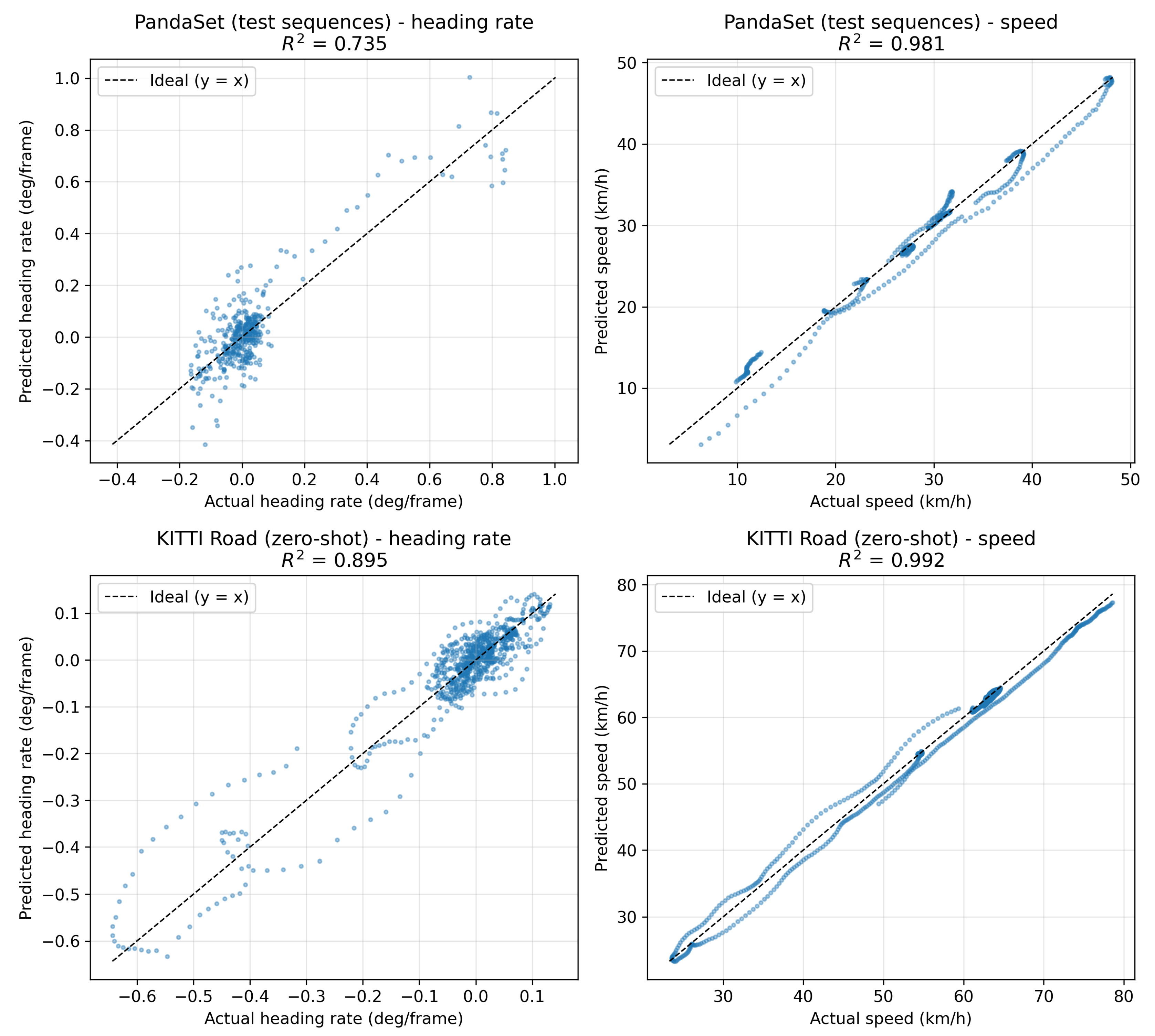
Figure 9.
Actual mean speed over the next 1 s and speed predicted by the CNN-LSTM with the physics term and by the persistence baseline along KITTI sequence 2011_09_26, drive 0015 (first split). The physical limit remained above the plotted range throughout the sequence.
Figure 9.
Actual mean speed over the next 1 s and speed predicted by the CNN-LSTM with the physics term and by the persistence baseline along KITTI sequence 2011_09_26, drive 0015 (first split). The physical limit remained above the plotted range throughout the sequence.
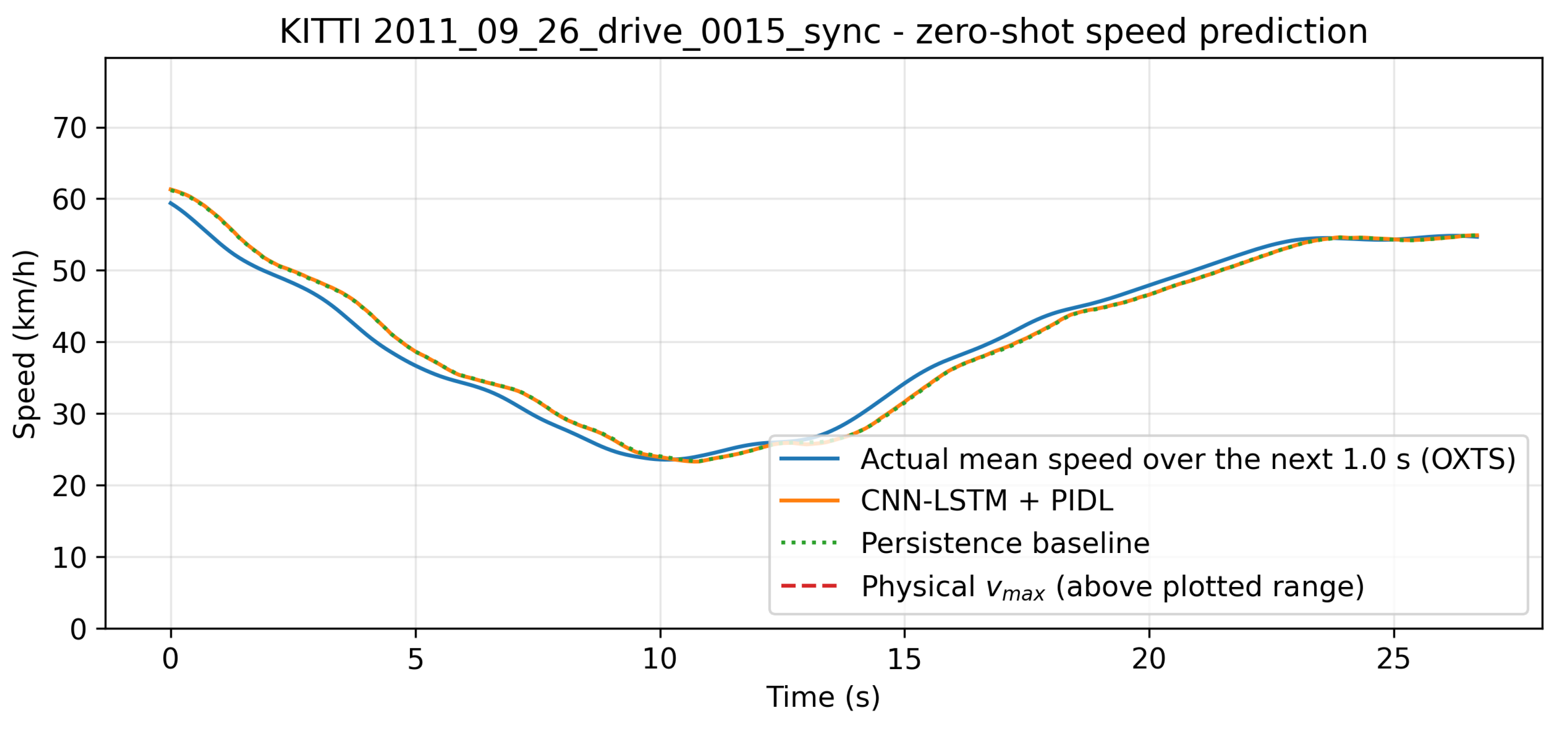

Table 1.
CNN-LSTM architecture and training configuration.
| Component | Configuration |
|---|---|
| Input | 20 frames × 8 features (standardized) |
| Convolution 1 | Conv1D, 32 filters, kernel 3, causal padding, ReLU |
| Convolution 2 | Conv1D, 16 filters, kernel 3, causal padding, ReLU |
| Recurrent layer | LSTM, 32 units, followed by dropout (0.3) |
| Shared layer | Dense, 16 units, ReLU, followed by dropout (0.3) |
| Outputs | Two linear heads: and (standardized) |
| Loss | , with |
| Optimizer | Adam (default learning rate), batch size 64 |
| Stopping | Early stopping on the validation loss (patience 10, maximum 100 epochs) |
Table 2.
Mean squared error of the persistence baseline and of the proposed model (CNN-LSTM with the physics term), as mean ± standard deviation over five splits. PandaSet values refer to the test sequences and KITTI values to zero-shot evaluation. is the relative change of MSE with respect to persistence (negative values indicate a lower error), with the number of splits in which the model obtained a lower MSE in parentheses. Heading-rate MSE is given in (deg/frame)2 and speed MSE in (km/h)2. KITTI persistence values do not vary across splits because the KITTI data are the same in every split.
Table 2.
Mean squared error of the persistence baseline and of the proposed model (CNN-LSTM with the physics term), as mean ± standard deviation over five splits. PandaSet values refer to the test sequences and KITTI values to zero-shot evaluation. is the relative change of MSE with respect to persistence (negative values indicate a lower error), with the number of splits in which the model obtained a lower MSE in parentheses. Heading-rate MSE is given in (deg/frame)2 and speed MSE in (km/h)2. KITTI persistence values do not vary across splits because the KITTI data are the same in every split.
| H (s) | Dataset | Heading rate | Speed | ||||
|---|---|---|---|---|---|---|---|
| Persistence | Model | (%) | Persistence | Model | (%) | ||
| 1 | PandaSet | 9.40±2.60 | 9.06±2.61 | −3.7±4.0 (5/5) | 2.19±0.84 | 1.80±0.56 | −15.7±16.1 (4/5) |
| 1 | KITTI | 1.97 | 2.08±0.22 | +5.4±11.0 (2/5) | 1.17 | 1.45±0.14 | +24.4±12.1 (0/5) |
| 2 | PandaSet | 11.85±4.01 | 10.05±4.41 | −16.4±20.1 (4/5) | 7.41±3.29 | 5.36±1.47 | −23.0±15.6 (5/5) |
| 2 | KITTI | 3.93 | 3.88±0.18 | −1.3±4.5 (4/5) | 4.04 | 5.69±1.82 | +40.8±45.0 (1/5) |
| 3 | PandaSet | 15.29±9.33 | 13.25±7.93 | −13.7±22.9 (3/5) | 15.14±7.43 | 10.57±3.96 | −27.0±10.0 (5/5) |
| 3 | KITTI | 5.26 | 5.28±0.71 | +0.5±13.6 (4/5) | 8.41 | 12.02±2.10 | +42.9±25.0 (0/5) |
Table 3.
Coefficient of determination () of the persistence baseline and of the proposed model (CNN-LSTM with the physics term), as mean ± standard deviation over five splits.
Table 3.
Coefficient of determination () of the persistence baseline and of the proposed model (CNN-LSTM with the physics term), as mean ± standard deviation over five splits.
| H (s) | Dataset | Heading rate | Speed | ||
|---|---|---|---|---|---|
| Persistence | Model | Persistence | Model | ||
| 1 | PandaSet | 0.06±0.61 | 0.08±0.61 | 0.981±0.005 | 0.985±0.003 |
| 1 | KITTI | 0.89 | 0.89±0.01 | 0.993 | 0.992±0.001 |
| 2 | PandaSet | −0.34±0.74 | −0.18±0.83 | 0.935±0.022 | 0.952±0.011 |
| 2 | KITTI | 0.77 | 0.77±0.01 | 0.978 | 0.968±0.010 |
| 3 | PandaSet | −0.69±0.67 | −0.52±0.85 | 0.863±0.056 | 0.903±0.032 |
| 3 | KITTI | 0.64 | 0.64±0.05 | 0.954 | 0.934±0.012 |
Table 4.
Qualitative comparison with representative approaches (different datasets and conditions).
| Method | Architecture | Evaluation Setting | Curve Handling | Physical Constraints | Reported Performance |
|---|---|---|---|---|---|
| MPC [6,9] | Model-based optimal control | Mainly simulation | Explicit (hard constraints) | Yes (vehicle model) | Depends on model fidelity |
| DRL (DDPG/PPO) [11,12] | Deep neural network (RL) | Simulation and real vehicle | Implicit (reward function) | No | High in simulation; sim-to-real gap |
| CNN perception [10] | Convolutional neural network | Urban speeds | Road detection only | No | No temporal continuity |
| CNN-LSTM + PIDL (this work) | Hybrid CNN-LSTM, multi-task | Offline, PandaSet and KITTI, five splits | LiDAR road preview at 10–40 m | Yes (soft penalty in the loss) | Speed MSE 16–27% below persistence (PandaSet); no gain on KITTI |
Disclaimer/Publisher’s Note: The statements, opinions and data contained in all publications are solely those of the individual author(s) and contributor(s) and not of MDPI and/or the editor(s). MDPI and/or the editor(s) disclaim responsibility for any injury to people or property resulting from any ideas, methods, instructions or products referred to in the content. |
© 2026 by the authors. Licensee MDPI, Basel, Switzerland. This article is an open access article distributed under the terms and conditions of the Creative Commons Attribution (CC BY) license (http://creativecommons.org/licenses/by/4.0/).
Copyright: This open access article is published under a Creative Commons CC BY 4.0 license, which permit the free download, distribution, and reuse, provided that the author and preprint are cited in any reuse.