

Submitted:
04 November 2026
Posted:
05 November 2026
You are already at the latest version
Abstract
This paper investigates the influence of phase inductance identification accuracy on the modelling and control performance of switched reluctance motors (SRMs). Fundamental motor equations and representative operating waveforms are presented to highlight the importance of inductance profiles in electromagnetic torque prediction and control strategy development. Experimental investigations reveal that the identified phase inductance depends on the excitation frequency used during measurement. This phenomenon is examined using a parameter-fitted Jiles–Atherton hysteresis model incorporating the influence of the magnetic circuit air gap. The experimentally observed relationship is reproduced in the model and approximated using a power-law function, enabling the recalculation of inductance profiles to improve their consistency with torque-based measurements. The original and recalculated inductance profiles are subsequently evaluated using five control strategies, including three model predictive control (MPC) approaches. Control performance is assessed using three quality indices describing torque tracking accuracy, peak-to-peak torque ripple, and maximum torque deviation. The comparative results support the hypothesis that the proposed inductance recalculation substantially improves SRM control performance, demonstrating the importance of accurate magnetic characteristics in advanced control strategies.
Keywords:
switched reluctance motor (SRM)
; phase inductance identification
; magnetic hysteresis
; Jiles–Atherton model
; frequency-dependent inductance
; model predictive control (MPC)
; torque ripple minimization
; torque control
1. Introduction
The switched reluctance motor (SRM) presented in the Figure 1, despite its advantages, including a simple construction and the absence of rare-earth materials, resulting in relatively low manufacturing costs, is inherently characterised by nonlinear energy conversion phenomena. This nonlinearity complicates the fundamental mathematical equations describing the generated electromagnetic torque.
If the flux linkage () is a nonlinear function of the phase current ():
where: – related to p-phase rotation angle, then the electromagnetic torque will be:
and the induced electromotive force (EMF):
The above relationship can be expressed in terms of the phase inductance ():
In the above formulation, the dependence on accounts for magnetic saturation effects. If these effects are negligible compared to other phenomena affecting the control system or due to the inherent characteristics of the motor, the governing equations can be simplified to:
and
This representation is particularly useful in control system design, where accurate modelling of the angular phase inductance profile and its derivative is essential for achieving high control performance [1]. It is also worth noting that, as an alternative to the physics-based modelling approach adopted in this study, data-driven methods, such as artificial neural networks (ANNs), are increasingly used [2].
Since the present study does not focus on magnetic saturation effects, a simplified model neglecting the current dependence of inductance is adopted. Instead, the article addresses another important magnetic phenomenon – hysteresis – which may significantly affect measured motor characteristics and, consequently, the accuracy of the resulting model [3].
As illustrated in Figure 2, even when the phase current is maintained at a constant level by the controller, the generated electromagnetic torque can vary considerably with rotor position. These variations adversely affect drive dynamics, increase mechanical stress, and contribute to acoustic noise. Importantly, the torque waveform depends not only on the nonlinear relationship between phase current and electromagnetic torque but also on the selected turn-on and turn-off angles, which provide additional degrees of freedom in the control process. However, the selection of these angles is constrained by other important drive performance requirements, particularly energy efficiency. Consequently, achieving accurate torque control while minimising torque ripple remains a challenging task in switched reluctance motor drives.
The article presents an efficient method for measuring the angular phase inductance profile . However, the resulting profile is subject to distortions caused by magnetic hysteresis [4]. The influence of this phenomenon is investigated and validated using an extended Jiles–Atherton model that incorporates the air gap of the magnetic circuit. Subsequently, a compensation method is proposed to correct the hysteresis-induced distortions, thereby improving the agreement between the identified inductance profile and experimental results.
To accurately represent the electromagnetic behaviour of the motor, the phase torque characteristic has been identified with high precision. This characteristic enables accurate reproduction of the electromagnetic torque and provides a basis for calculating the rotational back electromotive force:
The two inductance profiles, namely the raw measured profile and the recalculated profile, will then be used to compare control performance in the particularly challenging task of torque ripple minimisation. Torque ripple is an inherent characteristic of switched reluctance motors, primarily resulting from phase commutation and the nonlinear relationship between phase current and electromagnetic torque. The following control strategies will be considered [5]:
- (a)
- gain-scheduled PI controller with T->i model inversion and optimal turn-on and turn-off angles (GSPI-MI),
- (b)
- as above, but with simple Torque Sharing Mechanism (GSPI-MITSM),
- (c)
- Single-Move Torque MPC (SM-TMPC),
- (d)
- Backward-Planned Predictive Torque Control (BP-PTC),
- (e)
- Full-Horizon Torque MPC (FH-TMPC).
2. Raw aNgular Inductance Profile
2.1. Laboratory Setup
Figure 3 presents a dedicated laboratory test bench designed for fully automated measurement of the motor characteristics. The programmable measurement system enables two operating modes. In the first mode, voltage pulses are applied to the phase winding to excite its transient response, which is subsequently used to determine the angular inductance profile (). A comparable methodology was proposed in [6] . In the second mode, a controlled DC current is supplied to the phase winding to obtain the electromagnetic torque characteristic . All analogue signals are acquired using a remotely controlled oscilloscope communicating via an Ethernet interface. The recorded data are stored on a USB flash drive for subsequent processing on a PC. The rotor angular position can be precisely controlled by a mechanical drive system consisting of a stepper motor, a gearbox, and the tested SRM. A detailed description of the torque measurement procedure and system description is provided in [7].
2.2. Calculation
Once a series of current responses to voltage pulses has been recorded, signal averaging can be applied to improve the signal-to-noise ratio (SNR) and enhance the repeatability of the measurement results. All current record for given position are separated into single excitations with some signal cutting on the edge because of noise signification. It means that – in general – the time-signal relation is lost. So, the model that fit signal to exponential should take it into account. It might be done in two ways. One, by use time shift :
and the second by value shift :
However, if the voltage and resistance are known, Equation 8 can be linearised. First, the exponential term is isolated:
Taking the natural logarithm and multiplying by (-1):
define the transformed dependent variable:
then:
Therefore, the original parameters can be recovered from linear regression:
This approach is significantly less computationally demanding than fitting Equation (8) using a gradient-based optimisation method. Moreover, the resulting linear least-squares problem admits a unique global solution, provided that the parameter estimation problem is well-posed.
Representative results of fitting the phase current responses at rotor positions corresponding to approximately minimum and maximum inductance is presented in Figure 4. A systematic trend can be observed: the higher the inductance, the greater the discrepancy between the measured and fitted current waveforms. This discrepancy is not attributable to numerical fitting errors but rather to magnetic hysteresis in the motor’s magnetic circuit.
3. Jiles–Atherton Magnetic Circuit Model with an Air Gap
The Jiles–Atherton (J–A) model provides a physics-based approach to describing the nonlinear magnetization characteristics of ferromagnetic materials, including magnetic saturation and hysteresis [8]. The model distinguishes between reversible and irreversible magnetization mechanisms, associated primarily with magnetic domain wall displacement and pinning. Owing to its relatively small number of parameters and moderate computational complexity, the J–A model is suitable for numerical analysis of electromagnetic devices.
In magnetic circuits containing an air gap, the magnetization characteristics are influenced not only by the intrinsic properties of the ferromagnetic material but also by the additional magnetic reluctance introduced by the gap [9]. This effect can be incorporated into the J–A formulation through an effective demagnetizing coefficient, denoted by (). The coefficient represents the reduction in the internal magnetic field caused by the air-gap geometry and can be included in the effective field equation.
Introducing simplified air-gap coefficient:
where: – air gap length, – magnetic core length, the magnetic field strength in core material will be:
where: – overall magnetisation.
In the Jiles–Atherton (J–A) model, the anhysteretic magnetisation is defined as follows [8] [10]:
then irreversible one:
and reversible:
If total magnetization is:
then defining q:
the magnetization derivatives are:
and:
The magnetic flux density is then obtained as:
If define J-A typical model parameters:
then the parameters of the above model can be estimated using the Gauss–Newton method for nonlinear least-squares optimisation, with the parameter update calculated as follows:
where r – residual as measured minus predicted values:
where is the model sensitivity matrix, numerically approximated as:
Figure 5 presents the results of the Jiles–Atherton (J–A) model parameter fitting. The identified model provides significantly better agreement with the experimentally measured current waveforms than the simple exponential response predicted by a constant-parameter RL circuit model. The parameter fitting procedure converged successfully, yielding a good agreement between the model predictions and experimental data, as quantified by the goodness-of-fit statistic. The methodology underlying the proposed algorithm is based on the approach presented in [10]. The paper [11] presents an alternative approach to numerical identification of hysteresis parameters.
Experimental investigations revealed that, even at a fixed rotor position, the inductance estimated using the exponential fitting method depends on the excitation pulse repetition frequency. As illustrated in Figure 6, higher excitation frequencies result in lower estimated inductance values. Furthermore, the same trend was reproduced using the Jiles–Atherton (J–A) magnetic circuit model, supporting the conclusion that magnetic hysteresis is a major contributor to the observed frequency dependence.
4. Inductance Profile Recalculation
Since the motor phases generate electromagnetic torque under approximately constant-current conditions, the power-law function fitted to the frequency-dependent inductance data presented in Figure 6 can be extrapolated to zero excitation frequency to estimate the effective inductance under quasi-static conditions [12]. The proposed method is illustrated in Figure 7, where the extrapolated inductance corresponds to the intercept of the fitted function at zero frequency. For the adopted power-law approximation, this value is directly determined by the constant coefficient c (when ), as expressed below:
It is sufficient to perform measurements at several excitation frequencies for two characteristic rotor positions: the aligned position, corresponding to maximum inductance, and the unaligned position, corresponding to minimum inductance. The inductance values at all intermediate rotor positions lie within the range defined by these two extremes.
Figure 8 presents the results of the inductance profile recalculation using the method described above. Notably, the angular derivative of the recalculated inductance profile closely agrees with the reference characteristic derived from the experimentally measured torque profile . This demonstrates that the proposed correction is not merely a uniform scaling of the original inductance profile but also modifies its angular dependence.
5. Control Strategies
5.1. Introduction
Two phase inductance profiles will be used to develop and evaluate different control strategies: the original profile, obtained directly from the measured phase-current dynamics and denoted as data set A, , and the recalculated profile, denoted as data set B, . All considered control strategies aim to regulate the generated electromagnetic torque to a specified reference value , relying extensively on the corresponding inductance profiles. The paper [13] reviews various model predictive control (MPC) approaches for switched reluctance motor (SRM) drives, whereas [14] investigates MPC applied to synchronous reluctance motor (SynRM) drives.
5.2. Control Structure a (GSPI-MI)
The gain-scheduled PI current controller (block in Figure 9), combined with torque-to-current model inversion () and turn-on and turn-off angles optimised offline for minimum torque ripple, is employed as the baseline control strategy. Back-electromotive force (back-EMF) compensation and controller parameter tuning to compensate for the dominant electrical dynamics of the phase winding, with a control bandwidth approximately five times lower than the PWM switching frequency, provide good current tracking performance (Figure 10). However, the inherent limitations imposed by the winding current dynamics, combined with the absence of a mechanism accounting for overlapping phase currents and their cumulative contribution to the total electromagnetic torque, result in substantial torque peaks and poor overall torque control performance.
5.3. Control Structure b (GSPI-MITSM)
The second control strategy extends the baseline structure by introducing a torque-sharing (TS) block, as illustrated in Figure 11. This block adjusts the torque reference of the incoming phase by subtracting the electromagnetic torque generated by the outgoing phase from the total torque setpoint. Although this approach effectively eliminates excessive torque accumulation during phase commutation (the corresponding waveforms are presented in Figure 12), the limited current dynamics of the phase windings prevent the incoming phase current from accurately tracking its reference trajectory. Consequently, a temporary torque drop occurs during commutation, resulting in increased torque ripple.
5.4. Control Structure c (SM-TMPC)
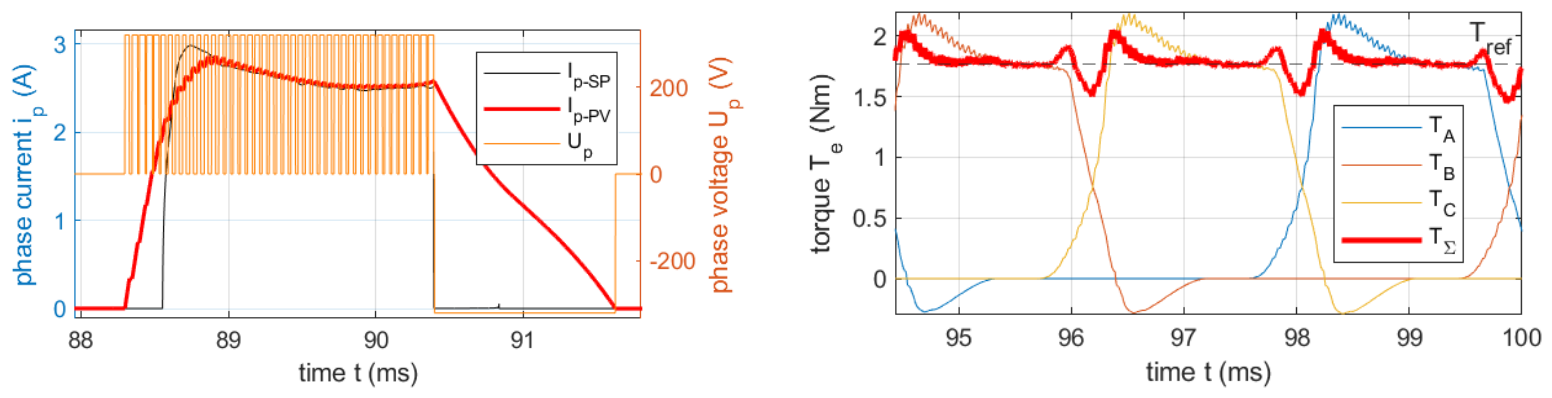
The proposed Single-Move Torque MPC (SM-TMPC) strategy is a simplified version of the approach presented in [17]. As illustrated in Figure 13, the control structure consists of two main functional blocks: the Demagnetisation Predictor (DP), responsible for predicting the torque contribution of the outgoing phase, and the Single-Move Torque Optimiser (SMT), which anticipates phase commutation and enables pre-magnetisation of the incoming phase winding. By optimising a single control variable over the entire prediction horizon, the computational complexity is substantially reduced. However, this simplification also limits the flexibility of the predicted control trajectory, potentially introducing a smoothing effect and reducing the dynamic response of the controller. Nevertheless, the resulting torque drops during phase commutation are considerably smaller than those observed with the previously discussed control strategies (Figure 14).
5.5. Control Structure d (BP-PTC)
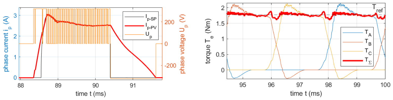
The proposed Backward-Planned Predictive Torque Control (BP-PTC) strategy is closely related to the approach presented in [18]. The algorithm evaluates the feasibility of achieving the required electromagnetic torque at the end of the prediction horizon and performs backward planning to determine the necessary control actions at preceding time steps. If the phase winding dynamics prevent the required torque from being achieved within the available time, the algorithm advances the excitation by propagating the required control action to earlier time steps. This mechanism compensates for the limited current dynamics by initiating phase pre-magnetisation, although it may temporarily produce excessive electromagnetic torque during this process. The strategy demonstrates good performance when combined with offline-optimised phase turn-on and turn-off angles (Figure 18).
Figure 15.
System schematic of the BP-PTC control structure.
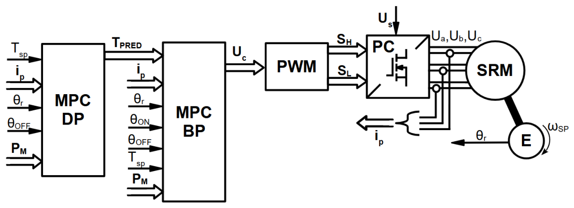
Figure 16.
Phase-current control waveforms (left) and resulting electromagnetic torque waveforms (right) for the BP-PTC control strategy.
Figure 16.
Phase-current control waveforms (left) and resulting electromagnetic torque waveforms (right) for the BP-PTC control strategy.
5.6. Control Structure e (FH-TMPC)
The proposed FH-TMPC strategy optimizes an independent control voltage for each step of the prediction horizon. Unlike Single-Move Torque MPC (SM-TMPC), which assumes a constant voltage over the entire horizon, FH-TMPC determines a sequence of future voltage commands while applying only the first command at the current control instant.
For the SRM commutation problem, the outgoing phase A is described by a demagnetization predictor, whereas the incoming phase B is controlled using quadratic programming (QP). The optimization minimizes a torque-sensitivity-weighted current tracking error, thereby approximating electromagnetic torque tracking while preserving the convex quadratic structure of the optimization problem. The alternative name for the algorithm will be: Torque-Sensitivity-Weighted Current MPC (TSW-CMPC).
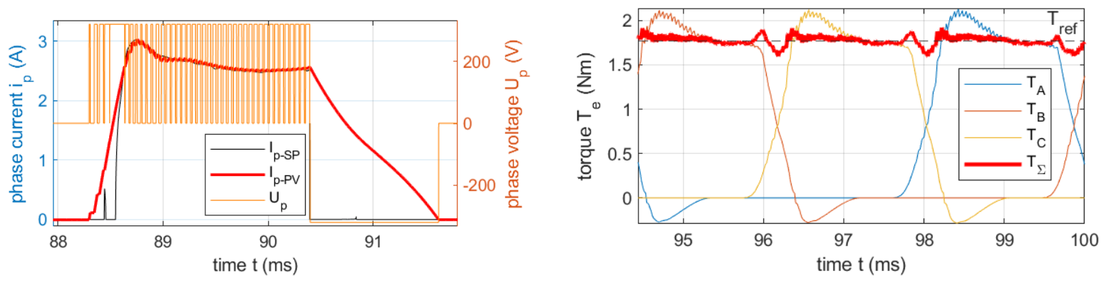
Compared with the backward-planning algorithm, the proposed control strategy provides smoother tracking of the reference current trajectory, as illustrated in Figure 18. However, for the adopted phase excitation angles, no substantial improvement in overall torque control performance was observed. Nevertheless, more pronounced benefits may emerge under different operating conditions, particularly during dynamic transients. The achieved control performance is already sufficiently high that inaccuracies in the underlying motor model become an increasingly important factor limiting further improvements.
Figure 17.
System schematic of the FH-TMPC control structure.
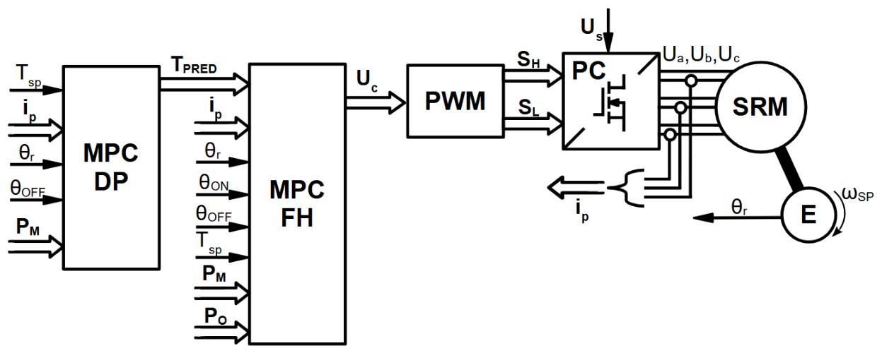
Figure 18.
Phase-current control waveforms (left) and resulting electromagnetic torque waveforms (right) for the FH-TMPC control strategy.
Figure 18.
Phase-current control waveforms (left) and resulting electromagnetic torque waveforms (right) for the FH-TMPC control strategy.
6. Results
6.1. Control performance metrics
To facilitate a clear comparison, three control performance indices are introduced to evaluate the deviation of the total electromagnetic torque from its reference value over the rotor angular interval from to :
Quality index — Mean squared relative torque error:
Quality index — Squared relative peak-to-peak torque ripple:
Quality index — Squared maximum relative torque deviation:
Superscripts are used to identify the inductance data set, either A (raw) or B (recalculated), followed by the control structure and strategy, denoted by letters a–e according to the classification provided above. For example, denotes the second control performance index , evaluated using data set B (recalculated inductance profile) and control strategy a (GSPI-MI).
6.2. Summary Tables
6.2.1. Relative Control Performance

Table 1.
Relative control performance based on the objective function ratio (%).
| – | 0.25 | 0.50 | 0.75 | 1.00 |
|---|---|---|---|---|
| 0.25 | 11 | 13 | 10 | 9 |
| 0.50 | 14 | 20 | 15 | 14 |
| 0.75 | 13 | 16 | 11 | 18 |
| 1.00 | 17 | 20 | 20 | 31 |
Table 2.
Relative control performance based on the objective function ratio (%).
| – | 0.25 | 0.50 | 0.75 | 1.00 |
|---|---|---|---|---|
| 0.25 | 54 | 59 | 73 | 48 |
| 0.50 | 67 | 53 | 64 | 63 |
| 0.75 | 54 | 58 | 63 | 61 |
| 1.00 | 48 | 57 | 60 | 59 |
Table 3.
Relative control performance based on the objective function ratio (%).
| – | 0.25 | 0.50 | 0.75 | 1.00 |
|---|---|---|---|---|
| 0.25 | 36 | 38 | 38 | 29 |
| 0.50 | 41 | 39 | 37 | 37 |
| 0.75 | 31 | 33 | 31 | 38 |
| 1.00 | 25 | 33 | 38 | 44 |
Table 4.
Relative control performance based on the objective function ratio (%).
| – | 0.25 | 0.50 | 0.75 | 1.00 |
|---|---|---|---|---|
| 0.25 | 9 | 7 | 7 | 7 |
| 0.50 | 9 | 13 | 15 | 10 |
| 0.75 | 10 | 14 | 21 | 24 |
| 1.00 | 18 | 30 | 14 | 33 |
Table 5.
Relative control performance based on the objective function ratio (%).
| – | 0.25 | 0.50 | 0.75 | 1.00 |
|---|---|---|---|---|
| 0.25 | 158 | 79 | 159 | 89 |
| 0.50 | 105 | 239 | 132 | 97 |
| 0.75 | 68 | 219 | 97 | 112 |
| 1.00 | 129 | 141 | 64 | 118 |
Table 6.
Relative control performance based on the objective function ratio (%).
| – | 0.25 | 0.50 | 0.75 | 1.00 |
|---|---|---|---|---|
| 0.25 | 72 | 52 | 45 | 43 |
| 0.50 | 64 | 68 | 50 | 40 |
| 0.75 | 43 | 72 | 58 | 80 |
| 1.00 | 57 | 53 | 32 | 122 |
Table 7.
Relative control performance based on the objective function ratio (%).
| – | 0.25 | 0.50 | 0.75 | 1.00 |
|---|---|---|---|---|
| 0.25 | 5 | 4 | 4 | 4 |
| 0.50 | 3 | 10 | 8 | 6 |
| 0.75 | 8 | 6 | 6 | 10 |
| 1.00 | 25 | 25 | 15 | 10 |
Table 8.
Relative control performance based on the objective function ratio (%).
| – | 0.25 | 0.50 | 0.75 | 1.00 |
|---|---|---|---|---|
| 0.25 | 53 | 28 | 34 | 64 |
| 0.50 | 35 | 111 | 94 | 91 |
| 0.75 | 55 | 66 | 72 | 117 |
| 1.00 | 82 | 110 | 112 | 104 |
Table 9.
Relative control performance based on the objective function ratio (%).
| – | 0.25 | 0.50 | 0.75 | 1.00 |
|---|---|---|---|---|
| 0.25 | 24 | 18 | 16 | 18 |
| 0.50 | 10 | 24 | 20 | 16 |
| 0.75 | 21 | 25 | 23 | 30 |
| 1.00 | 33 | 45 | 34 | 26 |
Table 10.
Relative control performance based on the objective function ratio (%).
| – | 0.25 | 0.50 | 0.75 | 1.00 |
|---|---|---|---|---|
| 0.25 | 8 | 5 | 5 | 5 |
| 0.50 | 4 | 9 | 3 | 2 |
| 0.75 | 3 | 2 | 2 | 2 |
| 1.00 | 7 | 7 | 2 | 2 |
Table 11.
Relative control performance based on the objective function ratio (%).
| – | 0.25 | 0.50 | 0.75 | 1.00 |
|---|---|---|---|---|
| 0.25 | 229 | 151 | 207 | 276 |
| 0.50 | 179 | 356 | 96 | 73 |
| 0.75 | 114 | 94 | 56 | 81 |
| 1.00 | 133 | 149 | 54 | 32 |
Table 12.
Relative control performance based on the objective function ratio (%).
| – | 0.25 | 0.50 | 0.75 | 1.00 |
|---|---|---|---|---|
| 0.25 | 84 | 26 | 26 | 26 |
| 0.50 | 22 | 82 | 21 | 11 |
| 0.75 | 13 | 12 | 8 | 11 |
| 1.00 | 29 | 43 | 10 | 5 |
Table 13.
Relative control performance based on the objective function ratio (%).
| – | 0.25 | 0.50 | 0.75 | 1.00 |
|---|---|---|---|---|
| 0.25 | 6 | 5 | 5 | 4 |
| 0.50 | 3 | 7 | 3 | 2 |
| 0.75 | 3 | 3 | 2 | 2 |
| 1.00 | 5 | 4 | 3 | 2 |
Table 14.
Relative control performance based on the objective function ratio (%).
| – | 0.25 | 0.50 | 0.75 | 1.00 |
|---|---|---|---|---|
| 0.25 | 157 | 158 | 206 | 257 |
| 0.50 | 111 | 341 | 97 | 88 |
| 0.75 | 98 | 123 | 89 | 86 |
| 1.00 | 74 | 121 | 73 | 39 |
Table 15.
Relative control performance based on the objective function ratio (%).
| – | 0.25 | 0.50 | 0.75 | 1.00 |
|---|---|---|---|---|
| 0.25 | 51 | 26 | 25 | 24 |
| 0.50 | 11 | 68 | 19 | 12 |
| 0.75 | 12 | 13 | 10 | 13 |
| 1.00 | 16 | 23 | 13 | 7 |
7. Discussion
Analysis of the results presented in the preceding tables indicates that, in nearly all investigated cases, control algorithms employing the recalculated angular inductance profile achieve better performance than those based on the original measured profile. These findings support the hypothesis that magnetic hysteresis can introduce substantial errors into inductance profile estimation, thereby degrading control performance. For the investigated motor and experimental setup, the proposed correction method based on power-law approximation provides substantial improvements. However, its applicability should be further evaluated using other motors with different magnetic characteristics [19].
The experimental investigations also confirmed that the phase inductance , estimated by exponential fitting of the current response, depends on the excitation frequency . Higher excitation frequencies result in inductance estimates that are less representative of the motor’s torque-producing characteristics. The Jiles–Atherton (J–A) model was successfully extended to incorporate the air gap of the magnetic circuit, achieving good agreement between simulated and experimentally measured current waveforms. Furthermore, the model reproduced the observed frequency dependence of the estimated inductance, supporting the hypothesis that magnetic hysteresis is a major contributor to this phenomenon. The extended J–A magnetic circuit model was found to be highly sensitive to the assumed air-gap length, with even submillimetre variations significantly affecting the simulated characteristics. Further improvements in model accuracy may be achieved by including additional parameters in the identification procedure, such as the effective air-gap length, measurement signal time offset, and geometric parameters (e.g., the effective motor tooth area contributing to flux linkage).
The experimental setup could be further improved by implementing a more sophisticated phase-current measurement system, for example, using a – modulator combined with a dedicated DFSDM (Digital Filter for Sigma-Delta Modulators) peripheral [20]. Additionally, the motor shaft should be mechanically locked during measurements, as even slight rotor displacement caused by the generated electromagnetic torque changes the rotor–stator alignment and the effective magnetic reluctance, potentially introducing significant errors into the identified characteristics.
The comparison of control structures presented in Table 16, Table 17 and Table 18 further indicates that model predictive control (MPC) algorithms generally provide superior control performance. Interestingly, structure d, Backward-Planned Predictive Torque Control (BP-PTC), achieves comparable or even better results than the more computationally demanding Full-Horizon Torque MPC (FH-TMPC) in many investigated cases. Under less demanding operating conditions, characterised by low rotational speed and low torque, Single-Move Torque MPC (SM-TMPC) appears to provide sufficient control performance.
Table 16.
Best control performance according to : control structure ID and corresponding performance index value.
Table 16.
Best control performance according to : control structure ID and corresponding performance index value.
| – | 0.25 | 0.50 | 0.75 | 1.00 |
|---|---|---|---|---|
| 0.25 | Bc (0.0028) | Bc (0.0022) | Bc (0.0021) | Bc (0.0020) |
| 0.50 | Bc (0.0015) | Be (0.0040) | Be (0.0021) | Be (0.0014) |
| 0.75 | Be (0.0019) | Be (0.0015) | Be (0.0013) | Be (0.0011) |
| 1.00 | Be (0.0028) | Be (0.0023) | Bd (0.0013) | Bd (0.0010) |
Table 17.
Best control performance according to : control structure ID and corresponding performance index value.
Table 17.
Best control performance according to : control structure ID and corresponding performance index value.
| – | 0.25 | 0.50 | 0.75 | 1.00 |
|---|---|---|---|---|
| 0.25 | Ad (0.0911) | Bc (0.0453) | Bc (0.0393) | Ad (0.0313) |
| 0.50 | Ad (0.0554) | Ae (0.0364) | Be (0.0713) | Bd (0.0511) |
| 0.75 | Ad (0.0629) | Bd (0.0500) | Bd (0.0436) | Bd (0.0409) |
| 1.00 | Be (0.0706) | Ae (0.0487) | Bd (0.0391) | Bd (0.0274) |
Table 18.
Best control performance according to : control structure ID and corresponding performance index value.
Table 18.
Best control performance according to : control structure ID and corresponding performance index value.
| – | 0.25 | 0.50 | 0.75 | 1.00 |
|---|---|---|---|---|
| 0.25 | Bc (0.0527) | Bc (0.0276) | Bc (0.0228) | Bc (0.0232) |
| 0.50 | Be (0.0181) | Bc (0.0393) | Be (0.0344) | Be (0.0186) |
| 0.75 | Be (0.0203) | Bd (0.0164) | Bd (0.0146) | Bd (0.0151) |
| 1.00 | Be (0.0306) | Be (0.0274) | Bd (0.0159) | Bd (0.0090) |
Future research could investigate the integration of an additional dynamic compensation module into the gain-scheduled PI control structure to provide phase pre-magnetisation and mitigate torque drops during commutation. Another promising direction is the development of hybrid MPC–PI control strategies that could reduce computational requirements by dynamically selecting the appropriate control algorithm according to operating conditions, similar to presented in paper [21] or [22]. Such hybrid approaches could also provide improved robustness by switching to a conventional PI controller when the MPC optimisation fails or becomes computationally infeasible.
Author Contributions
Conceptualization, T.P. and B.F.; methodology, B.F.; validation, T.P. and B.F.; formal analysis, T.P. and B.F.; investigation, B.F.; resources, B.F.; data curation, T.P. and B.F.; writing—original draft preparation, B.F.; writing—review and editing, T.P. and B.F.; visualization, B.F.; supervision, T.P.; project administration, T.P. All authors have read and agreed to the published version of the manuscript.
References
- Surus, R.; Tejer, M.; Tarczewski, T. An Impact of Switching Frequency and Model Accuracy on Model Predictive Current Control Performance for Reluctance Synchronous Motors. Power Electron. Drives 2024, 9, 176–190. [Google Scholar] [CrossRef]
- Kamiński, M.; Tarczewski, T. Neural Network Applications in Electrical Drives—Trends in Control, Estimation, Diagnostics, and Construction. Energies 2023, 16, 4441. [Google Scholar] [CrossRef]
- Melo, P.; Pereira, M.; Araújo, R.E. Analysis of Static Magnetic Hysteresis Impact on a Switched Reluctance Motor Drive Controller; 2019; pp. 916–921. [Google Scholar] [CrossRef]
- Melo, P.; Araújo, R.E. Modeling and Simulation of a Switched Reluctance Motor with Hysteresis Effect; 2018; pp. 1303–1308. [Google Scholar] [CrossRef]
- Cai, J. Model Predictive Control Strategies in Switched Reluctance Motor Drives—An Overview. IEEE Trans. Power Electron. 2025, 40, 1669–1685. [Google Scholar] [CrossRef]
- Shao, D.; Gong, L.; Li, B.C.; Liu, C.L. Inductance Measurement of the Switched Reluctance Motor with the Current Traversal Response for Exciting Voltage Pulse. IFAC Proc. Vol. 2013, 46, 190–196. [Google Scholar] [CrossRef]
- Fabiański, B.; Pajchrowski, T.; Zawirski, K. Electronic system and signal processing in torque-meter interface of switched reluctance motor drive laboratory test bench. Przegląd Elektrotechniczny 2024, R. 100, nr 11. [Google Scholar] [CrossRef]
- Jiles, D.C.; Atherton, D.L. Theory of ferromagnetic hysteresis. J. Magn. Magn. Mater. 1986, 61, 48–60. [Google Scholar] [CrossRef]
- Surdacki, P.; Wozniak, L. Influence of the HTS Winding Tape on Limiting the Transient Currents in Superconducting Transformers. Energies 2022, 15, 1688. [Google Scholar] [CrossRef]
- Szewczyk, R. Computational Problems Connected with Jiles-Atherton Model of Magnetic Hysteresis. In Proceedings of the Recent Advances in Automation, Robotics and Measuring Techniques; Szewczyk, R., Zieliński, C., Kaliczyńska, M., Eds.; Cham, 2014; pp. 275–283. [Google Scholar] [CrossRef]
- Petrun, M.; Rahmanović, E. Parameter Estimation for the Basic Zirka-Moroz History-Dependent Hysteresis Model for Electrical Steels. Materials 2025, 18, 2104. [Google Scholar] [CrossRef] [PubMed]
- Chwastek, K.R. The Effects of Sheet Thickness and Excitation Frequency on Hysteresis Loops of Non-Oriented Electrical Steel. Sensors 2022, 22, 7873. [Google Scholar] [CrossRef] [PubMed]
- Zhu, Y.; Yao, M.; Sun, X. A Review on Predictive Control Technology for Switched Reluctance Motor System. World Electr. Veh. J. 2023, 14, 221. [Google Scholar] [CrossRef]
- Niewiara, L.J.; Surus, R.; Tarczewski, T. Computationally Efficient Gradient Enhanced FCS-MPCC With Reduced Torque Ripple for a Reluctance Synchronous Motor Drive. IEEE Trans. Ind. Electron. 2026, 73, 5198–5210. [Google Scholar] [CrossRef]
- Abdel-Aziz, A.; Elgenedy, M.; Williams, B. A New Torque Control Approach for Torque Ripple Minimisation in Switched Reluctance Drives. Energies 2024, 17, 3334. [Google Scholar] [CrossRef]
- Fabianski, B. Optimal control of switched reluctance motor drive with use of simplified, nonlinear reference model. In Proceedings of the 2016 17th International Conference on Mechatronics - Mechatronika (ME), 2016; pp. 1–8. [Google Scholar]
- Shen, S.; Wang, H.; Feng, Y.; Li, M.; Zhong, Y. Predictive Current Control for Switched Reluctance Motor Based on Local Linear Phase Voltage Model. Appl. Sci. 2022, 12, 1688. [Google Scholar] [CrossRef]
- Sheng, L.; Wang, G.; Fan, Y.; Liu, J.; Liu, D.; Mu, D. An Improved Direct Predictive Torque Control for Torque Ripple and Copper Loss Reduction in SRM Drive. Appl. Sci. 2023, 13, 5319. [Google Scholar] [CrossRef]
- Melo, P.; Araújo, R.E. Modeling a Switched Reluctance Motor with Static Magnetic Hysteresis: Impact on High-Speed Operation. 2018. [Google Scholar] [CrossRef]
- Ewert, P.; Pajchrowski, T.; Wicher, B. Sensorless Detection of Mechanical Unbalance in Servodrive with Elastic Coupling. Energies 2024, 17, 4859. [Google Scholar] [CrossRef]
- Li, L.; Wu, J.; Yang, Y.; Guo, Z.; Wang, H.; Li, S. Cooperative MPC-DITC Strategy for Torque Ripple Suppression in Switched Reluctance Motors. World Electr. Veh. J. 2026, 17, 154. [Google Scholar] [CrossRef]
- Frański, A.; Horla, D.; Iervolino, R. On Increasing the Energy Efficiency and Performance of a Bicycle Robot Stabilization—Towards Event-Triggered Control Considerations. Energies 2025, 18, 6146. [Google Scholar] [CrossRef]
Figure 1.
Switched reluctance motor: (a) cross-sectional view and (b) photograph of the disassembled motor.
Figure 1.
Switched reluctance motor: (a) cross-sectional view and (b) photograph of the disassembled motor.
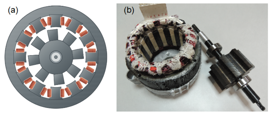
Figure 2.
Representative waveforms of phase voltage, current, inductance, and electromagnetic torque in an SRM.
Figure 2.
Representative waveforms of phase voltage, current, inductance, and electromagnetic torque in an SRM.
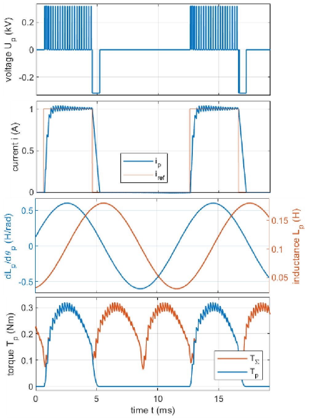
Figure 3.
Experimental setup for measuring the SR-motor characteristics.
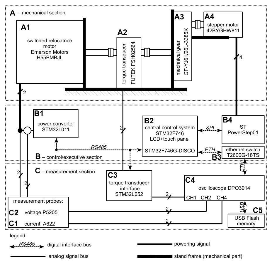
Figure 4.
Phase currents at voltage pulse excitation with fitting results in different rotor positions.
Figure 4.
Phase currents at voltage pulse excitation with fitting results in different rotor positions.
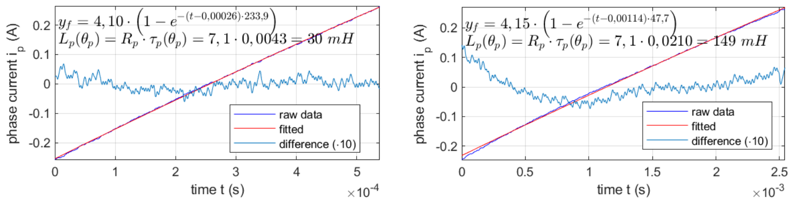
Figure 5.
Experimental and Jiles–Atherton-modelled current responses to voltage-pulse excitation for the equivalent inductance , at 200 Hz (top) and 50 Hz (bottom).
Figure 5.
Experimental and Jiles–Atherton-modelled current responses to voltage-pulse excitation for the equivalent inductance , at 200 Hz (top) and 50 Hz (bottom).
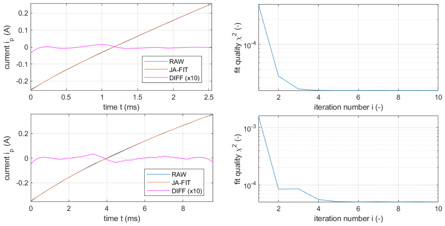
Figure 6.
Inductance estimated by exponential fitting as a function of the excitation pulse frequency.
Figure 6.
Inductance estimated by exponential fitting as a function of the excitation pulse frequency.
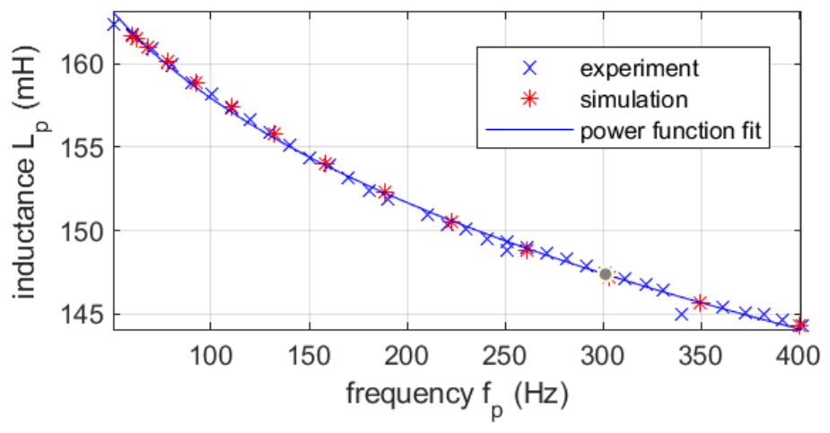
Figure 7.
Inductance estimated at different phase-winding excitation frequencies.
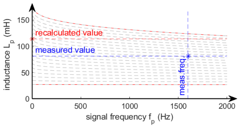
Figure 8.
Recalculated inductance profile and its angular derivative compared with those derived from torque measurements.
Figure 8.
Recalculated inductance profile and its angular derivative compared with those derived from torque measurements.
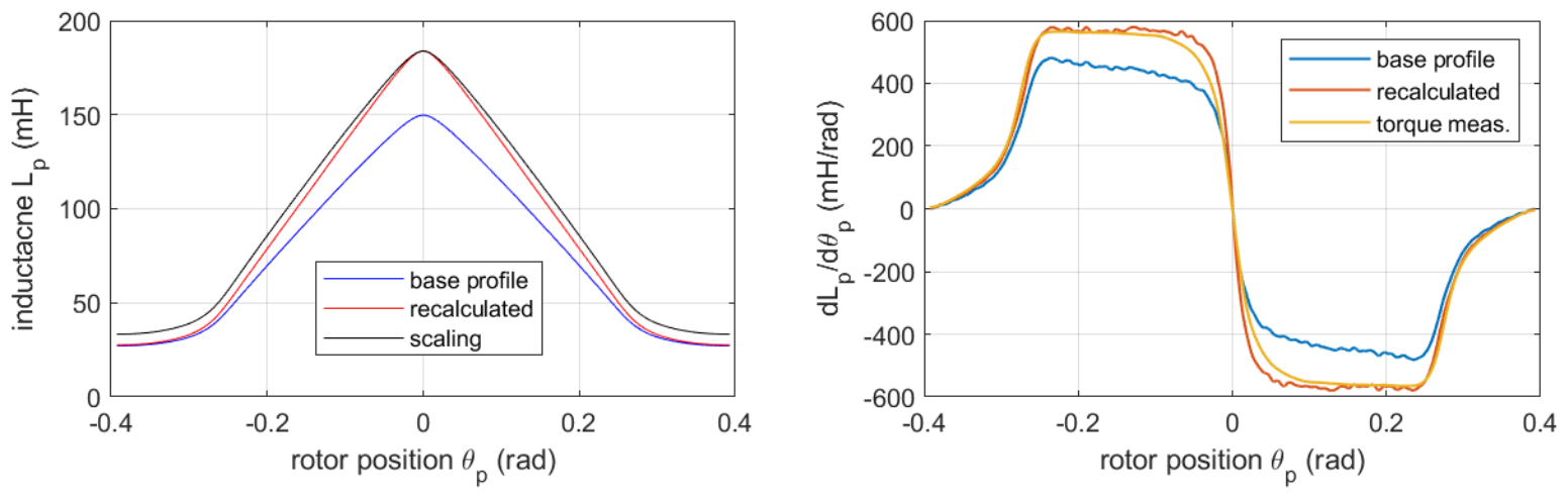
Figure 9.
System schematic of the GSPI-MI control structure.
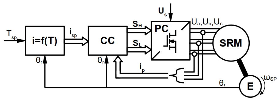
Figure 10.
Phase-current control waveforms (left) and resulting electromagnetic torque waveforms (right) for the GSPI-MI control strategy.
Figure 10.
Phase-current control waveforms (left) and resulting electromagnetic torque waveforms (right) for the GSPI-MI control strategy.
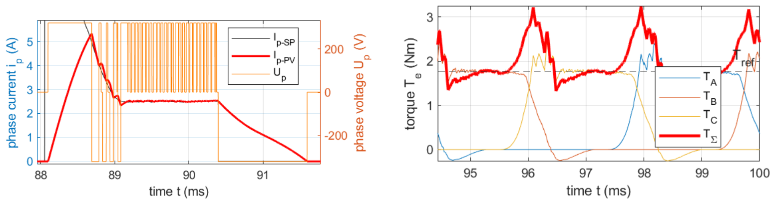
Figure 11.
System schematic of the GSPI-MITSM control structure.
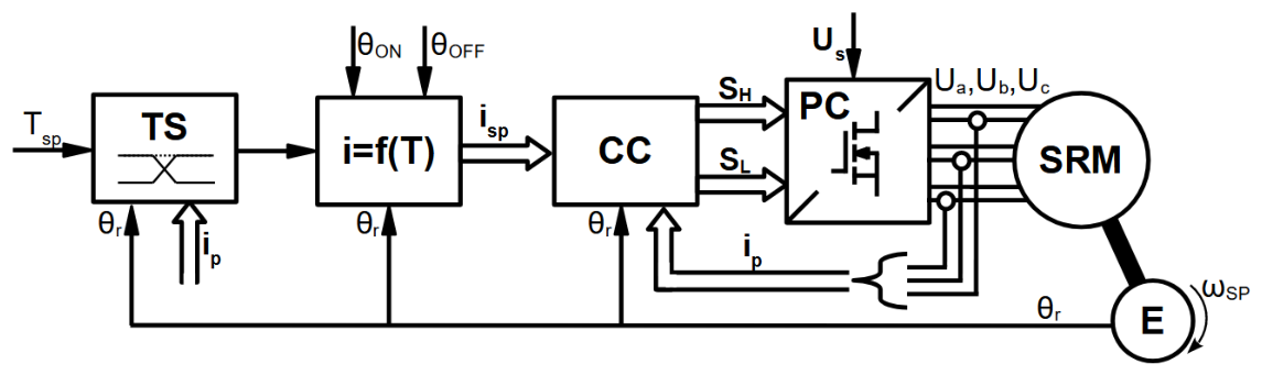
Figure 12.
Phase-current control waveforms (left) and resulting electromagnetic torque waveforms (right) for the GSPI-MITSM control strategy.
Figure 12.
Phase-current control waveforms (left) and resulting electromagnetic torque waveforms (right) for the GSPI-MITSM control strategy.
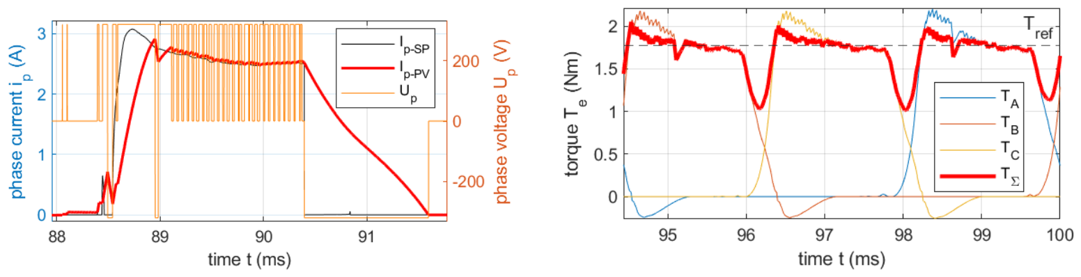
Figure 13.
System schematic of the SM-TMPC control structure.
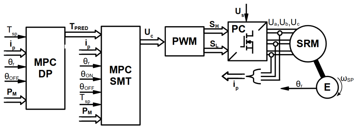
Figure 14.
Phase-current control waveforms (left) and resulting electromagnetic torque waveforms (right) for the SM-TMPC control strategy.
Figure 14.
Phase-current control waveforms (left) and resulting electromagnetic torque waveforms (right) for the SM-TMPC control strategy.
Disclaimer/Publisher’s Note: The statements, opinions and data contained in all publications are solely those of the individual author(s) and contributor(s) and not of MDPI and/or the editor(s). MDPI and/or the editor(s) disclaim responsibility for any injury to people or property resulting from any ideas, methods, instructions or products referred to in the content. |
© 2026 by the authors. Licensee MDPI, Basel, Switzerland. This article is an open access article distributed under the terms and conditions of the Creative Commons Attribution (CC BY) license (http://creativecommons.org/licenses/by/4.0/).
Copyright: This open access article is published under a Creative Commons CC BY 4.0 license, which permit the free download, distribution, and reuse, provided that the author and preprint are cited in any reuse.