

Submitted:
04 November 2026
Posted:
05 November 2026
You are already at the latest version
Abstract
AMMAP on CAS500-3, launched in November 2025 into a ∼600 km Sun-synchronous orbit, combines a Langmuir probe (LP), biased with respect to the spacecraft body, and an impedance probe (IP), which derives the density from the upper-hybrid resonance regardless of the spacecraft potential. We report the operation from December 2025 to June 2026 and initial observations on two reference days in February and June. Before the orbital noon, the sun-pointing attitude turns the solar arrays toward the direction of flight and the spacecraft charges negatively beyond the LP sweep range, so that the LP collects only ions in 50–70% of the dayside sweeps. The IP is lost mainly in the low-density winter hemisphere, where its resonance is too weak. Where both are valid, the densities agree within a factor of ∼1.7 in the median, the IP typically 20–40% lower; both lie above the IRI model, the IP by a factor of 1.4–2.1 and the LP by 2.1–3.2. Even in the ion-only sweeps, the slope of the ion current increases with the density and, calibrated against the IP for each day, gives the density with a scatter of 20–35%. Taking the IP as the reference and filling its gaps with the calibrated LP data yields a continuous profile over more than 90% of the two orbits examined.
Keywords:
ionosphere
; Langmuir probe
; impedance probe
; electron density
; spacecraft charging
; in-orbit calibration
1. Introduction
In situ plasma measurements from low-Earth-orbit (LEO) spacecraft have relied on the Langmuir probe (LP) for more than half a century, since one current–voltage (I–V) sweep of a simple electrode gives the electron density () and temperature () [1,2]. The LP current, however, returns through the spacecraft body, whose potential with respect to the plasma is neither known nor constant: it is set by the currents collected by the whole conducting surface, including the exposed interconnects of the solar array [3,4]. On a spacecraft, the characteristic may therefore shift partly or entirely out of the sweep range [5,6], and the absolute LP density generally depends on an external reference [7].
The impedance probe (IP), on the other hand, measures the impedance of a short antenna against frequency, and the upper-hybrid resonance, , gives the absolute density from the plasma frequency and the electron cyclotron frequency , regardless of the surface condition and the spacecraft potential [8,9,10,11,12]. The IP is thus expected to provide a platform-independent density reference, while the LP provides and a finer time resolution; this combination was proposed for CAS500-3 (Compact Advanced Satellite 500-3) and tested in a plasma chamber before launch [5,13].
IAMMAP (Ionospheric Anomaly Monitoring by Magnetometer and Plasma-probe) is a scientific payload aboard CAS500-3 [5,13,14]. IAMMAP consists of a magnetometer and a plasma instrument package, AIPIM (Advanced Impedance Probe for Ionospheric Monitoring), which integrates the LP and the IP. This paper focuses on the determination of electron density from the complementary measurements of the LP and IP, with particular emphasis on minimizing platform-dependent effects. The magnetometer observations will be reported separately. CAS500-3 was launched aboard the Korean launch vehicle KSLV-II in November 2025 into a Sun-synchronous orbit at an altitude of ∼600 km, with a local time of ascending node (LTAN) of ∼12:30. We present the operation of IAMMAP from December 2025 to June 2026 and the initial observations of the two probes (Section 2, Section 3 and Section 4), followed by the discussion and the summary (Section 5 and Section 6).
2. The Plasma Instruments of IAMMAP and the CAS500-3 Mission
IAMMAP (Figure 1) consists of an electronics box, the AIPIM sensor box ( mm) with the LP and the IP, and the three fluxgate sensor heads of AIMAG (Adaptive In-phase Magnetometer) [14]. The LP is a planar disk 25.4 mm in diameter with a guard ring whose current is not measured [13], and the IP antenna a short monopole (∼12 cm long, ∼4 mm in diameter). AIPIM is mounted on the nadir-side () platform, and both probes look sideways (), perpendicular to the direction of flight () and to the nadir in the nominal attitude (Figure 1c). The solar arrays are deployed on the opposite, zenith-facing side (), which therefore faces the Sun in the sun-pointing attitude (Section 4.4). In the following, we refer to the side as the solar-array side and to the side as the nadir side, and describe the attitude by the directions in which the solar arrays, the nadir side, and the sideways-looking LP disk face relative to the direction of flight (ram) and the Sun. The LP biases the disk with respect to the spacecraft body and measures the current through a transimpedance amplifier (TIA; 500 k) and a 16-bit analog-to-digital converter over V [13]; the TIA output is inverted in sign, which is undone in the analysis, and the sweep waveform, range, and sampling rate are programmable by on-board observation records. The IP applies a frequency sweep to the antenna through a capacitance bridge, whose output is detected by a heterodyne receiver and a logarithmic amplifier [5]; the impedance maximum at the upper-hybrid resonance appears as a dip in the bridge output [11]. Table 1 lists the parameters as operated. AIMAG, three tri-axial fluxgate sensors with a resolution better than 1 nT [14,15], was operated throughout the period, and its calibration is in progress.
3. Launch and Early-Orbit Operation
3.1. Operation Timeline
IAMMAP was first powered on for the Initial Activation and Check-out on 5 December 2025 (Figure 2). The In-Orbit Test (IOT), from mid-December 2025 to January 2026, confirmed the reception of the S-band science data and selected the dayside and nightside parameters of the plasma probes from 22 orbits with 20 parameter sets (Section 3.2); the IOT telemetry in the database covers 8–10 January 2026. After the normalization of the spacecraft in January, the routine payload operation started on 5–6 February, and the Day/Night scenario has been operated since March 2026. The spacecraft entered the safe-hold mode on 12 May at 17:47 UT, and IAMMAP resumed on 11 June at 04:11 UT. The packet loss of the science data was about 2% in the IOT and below 0.12% per month afterward, and their 136 samples per LP sweep were shown before launch to suffice for fitting the characteristic [13]. In total, the science data of 118 (LP) and 119 (IP) days and the ancillary data (position, velocity, and attitude quaternion at 1 Hz) of 180 days were archived from January to June 2026.
3.2. Day/Night Scenario and Parameter Selection
Since the density differs by an order of magnitude between day and night, the probes use two parameter sets, switched by absolute-time commands at the boundaries between the operational dayside, i.e., the ascending (noon) half of the orbit between and , and the nightside (Figure 1c). Since the dayside reaches 6–9 MHz in the equatorial region, the IP sweeps 0.1–10 MHz on the dayside and 0.1–5 MHz on the nightside, with 1 s per leg (∼7 km). The LP sweeps from to V with respect to the spacecraft body on both sides. One sweep, consisting of a rising half (up-leg) and a falling half (down-leg), takes 0.1 s, but only the first sweep of every 2 s (∼15 km) is transmitted, so that each transmitted sweep is a snapshot over ∼0.8 km.
3.3. Ground Data-Processing System
The ground data-processing system (1) generates the absolute-time command sequences of the Day/Night scenario from the predicted orbit, (2) parses the telemetry packets and aligns their GPS (Global Positioning System) time tags, (3) stores the science data, the state-of-health (SOH) telemetry, and the ancillary data in a relational database (∼ records by the end of the period), and (4) provides an interactive viewer linked to the database. The viewer shows the data of each packet with the position, the sunlight condition, the attitude, and the key SOH telemetry, and its LP and IP fitting tools implement the procedures of Section 4.1 and Section 4.2, so that each fit can be examined before the procedures are applied to the whole data set. Level-0 data are the time-aligned telemetry converted to the TIA output (LP) and the bridge output (IP); Level-1 data, and from the LP and from the IP, are in progress, and the results presented here are based on Level 0 and the prototype Level-1 tools.
4. Initial Observations of the Plasma Probes
Two reference days were selected: 7 February 2026, the earliest day with complete LP, IP, and ancillary data, which lies about midway between the December solstice and the March equinox, and 21 June 2026, the June solstice. Both are observed at nearly the same local times (∼12:30 and ∼00:30 LT), and they have the smallest and nearly the largest fractions of the dayside LP sweeps lost to spacecraft charging (about a half and two thirds; Section 4.5). In the Level-0 data, the LP current shows one excursion per transmitted sweep, deep on the dayside and shallow on the nightside, but on 21 June the dayside excursions are almost absent in the southern part of each pass, where the spacecraft is charged so negatively that the probe collects only ions over the whole sweep (Section 4.4). We call these sweeps ion-only sweeps, as opposed to the normal sweeps that keep the electron part of the characteristic, and a continuous stretch of ion-only sweeps along the orbit an ion-only interval. The IP bridge output dips at the resonance most deeply in the dense dayside equatorial region of 7 February, whereas such dips are hardly seen on 21 June, consistent with the lower dayside density of June (Section 4.3).
4.1. Langmuir Probe: Reconstruction and Fitting of the I–V Curves
Since the sweep voltage is not transmitted, the I–V curve is reconstructed from the timing of the sweep. The current is with k. Each packet holds 136 consecutive samples (one sweep period), and the sweep maximum ( V) is a sharp extremum of the current, located with sub-sample precision; the 68 samples before and after it form the up-leg and the down-leg, and each sample is assigned the voltage of its phase relative to the maximum. Samples at the TIA limit ( V) are excluded.
The curves are analyzed by the classical graphical method [2,16], in which a straight line is fitted to each of the three parts of the curve: the ion-saturation part at low voltages, the electron-retarding part just above the floating potential , where the electron current grows exponentially, and the electron-saturation part above the bend of the curve (the knee); the last two are fitted in . The ion line is fitted over the lowest 35% of the sweep, without the five samples next to the sweep minimum, where the sweep departs from the ideal triangle, and subtracted to give the electron current ; the retarding line is drawn through three points above , and its slope gives ; and the saturation line is drawn through six consecutive points above the knee. The plasma potential is the intersection of the two electron lines, and
where is the saturation current at and A the disk area. A fit is accepted when the current crosses zero within the sweep, the goodness of fit (GoF; coefficient of determination in ) is at least 0.9, lies at least 0.3 V below the top of the sweep, is between 500 and 10,000 K, and the saturation line is less than 30% as steep as the retarding line.
Equation (1) is the planar-probe expression: at the probe draws the random thermal flux of the electrons, which does not depend on the probe geometry, over the collecting area, here the front face of the disk. The geometry matters above . While the current of an ideal planar probe saturates there, that of a cylindrical or spherical probe keeps rising, because its sheath expands with the bias or, when the sheath is thick compared with the probe, because of the orbital motion of the electrons, as described by the orbital-motion-limited (OML) theory [16]. The present disk is intermediate: the Debye length is 5–10 mm at – and 2,000 K, so that the sheath, a few Debye lengths thick and growing with the bias, is comparable to or larger than the disk radius (12.7 mm). Hence, the current keeps rising above the knee, and a line fitted close to the knee is too steep and underestimates and . We therefore fit the saturation line at least 4 above , or as far above it as the top of the sweep allows, where the density depends on the position of the fitted points by only ∼10% per . In a plasma chamber, a disk LP of the same type, analyzed by the graphical method, gave densities compatible with the IP, but dependent on the voltage interval of the fitted lines [5]. The remaining dependence on the method is absorbed by the in-orbit calibration against the IP (Section 4.7), whose absolute level is in turn checked against the IRI (International Reference Ionosphere) model.
Figure 3 shows a dayside and a nightside sweep of 7 February, and Table 2 lists these and two sweeps of 21 June, all typical low-latitude sweeps whose is closest to the median of the region on that day. The dayside up-leg shows the textbook characteristic, with an exponential rise above V and the electron saturation above V (GoF = 0.99). On the dayside, and are higher by ∼1.5 V, i.e., the spacecraft is charged more negatively in these sunlit sweeps, with the Sun above its solar-array side (Section 4.4). The dayside of ∼ lies in the range expected for the daytime topside ionosphere at 600 km, and of ∼1,800–2,300 K lies near or below the lower end of the typical daytime range of 2,000–3,500 K [17]. The nightside , derived from three points spanning only ∼0.24 V above , is sensitive to the voltage resolution; being comparable to or higher than the dayside value, opposite to the usual behavior of the topside, it is regarded as an upper limit.
The down-leg of each sweep, measured ∼50 ms after the up-leg (e.g., Figure 3b,c), tests the hysteresis of the probe and the reconstruction of the sweep, since a difference between the two legs is expected to be instrumental. Over the two reference days, the two legs give essentially the same results (Figure 4a,b,d,e): the median down-to-up ratios of and are within 3% of unity, with a scatter of only 4–5% in and 7–9% in , and and are higher on the down-leg by only ∼0.1 V. The hysteresis is thus negligible, and the two legs are independent samples of the same plasma.
4.2. Impedance Probe: Upper-Hybrid Resonance and Electron Density
The IP sweep is synchronized to GPS time, and the first of the two sweeps in each 4-s packet is used, i.e., one up-leg and one down-leg every 4 s. The resonance is detected on a smooth polynomial fitted to each 31-sample leg as its deepest significant local minimum, and legs that deviate from their neighbors within ±60 s by more than a factor of 1.4 are rejected. The value of is then read near the polynomial minimum from a Savitzky–Golay curve [18], which follows the narrow, asymmetric dip more closely. The sweep range is not contained in the packet, and some nightside passes were swept over 0.1–10 MHz instead of the scheduled 0.1–5 MHz; read with the scheduled frequency axis, such a pass shows an apparent halved at its boundaries. The range of each nightside pass is therefore determined from the continuity of across its boundaries, as confirmed by the SOH telemetry of the IP on 30 March.
The density follows from the resonance condition of a short antenna at an angle to the magnetic field, with [8], and with in MHz [11]; the field is taken from the IGRF-14 (International Geomagnetic Reference Field) model [19] and from the attitude. Since reaches 0.1–0.4 on the dayside and 0.2–0.7 on the nightside, the magnetic field is included throughout. In most of the orbit the antenna is within ∼25° of perpendicular to the field, where the angle changes the density by less than 3%, but by up to ∼40% at the poleward ends of the nightside passes and in the tilted sun-pointing attitude. Where approaches , at the lowest nightside densities of the winter hemisphere, becomes the small difference of two nearly equal quantities, and the identification of the dip itself becomes uncertain. In the example of Figure 5, the dayside up-leg has a deep dip at MHz ( ) and the nightside up-leg at 3.62 MHz ( ); the down-legs, measured 1 s later, agree within 2%, and over the whole days the median of the two legs differs by less than 3% (Figure 4c,f). Table 3 lists the IP results at the times of the LP sweeps of Table 2, where the IP density is lower than the LP density by 30–50%. A small fraction (1–2%) of the accepted legs of 21 June, in the low-density winter regions, show at nearly fixed frequencies regardless of the surrounding density; these are thought to be spurious (Section 5).
4.3. Electron Density Along the Orbit from the Two Probes
For all up-legs of the two reference days, the two probes give the profiles of Figure 6 and the latitudinal distributions of Figure 7; the operational dayside and nightside are shown in orange and blue throughout this paper. The IP resonance is accepted in two thirds to three quarters of the ∼21,500 up-legs of each day, and the LP fit is valid in 30–45% of the dayside and ∼80% of the nightside up-legs. Where both are available, the two densities follow each other along the orbit, although the IP density is generally lower (Section 4.6). The dayside (∼12:30 LT) density exceeds the nightside density by a factor of 5–6 at low latitudes but only slightly at 50–60° in the summer hemisphere, and on 7 February most dayside passes show the two crests of the equatorial ionization anomaly (EIA) on either side of the magnetic equator. Within , the median IP density is ∼ and ∼ on the dayside and ∼ and ∼ on the nightside of the two days, and the nightside density is clearly higher in the summer hemisphere on both days. The lower dayside density of June may be related to the seasonal variation of the topside ionosphere. During the last solar minimum, the dayside maps of DEMETER at 660 km, an altitude similar to that of CAS500-3, show a lower density at low latitudes in the northern summer than in the other seasons, although the seasonal behavior differs with altitude [20]. Since only two days are compared here, the seasonal variation will be examined when more than a year of data has been accumulated.
The two probes fail in different places. The LP is lost in the southern part of every dayside pass, where the spacecraft is charged beyond the sweep range (Section 4.4), for a minute or two after each ion-only interval, and at the lowest nightside densities, below ∼ , in the troughs of the winter hemisphere. The IP depends not on the spacecraft potential but on the depth of the dip, which decreases with the density: on the nightside, the resonance is accepted in more than 90% of the sweeps at – but in only about a third at – , and on the 0.1–10 MHz sweeps a resonance below 1.6 MHz ( ) lies outside the searched range. The IP is therefore lost mainly in the low-density winter hemisphere. In the southern part of the sunlit passes of June, the two probes fail together, whereas on 7 February the IP is accepted in most of the ion-only dayside sweeps south of .
4.4. Spacecraft Charging and Attitude
In a large fraction of the dayside sweeps, the electron part of the characteristic is entirely missing, and the probe collects only ions over the whole sweep. On 21 June (Figure 8a), the peak-to-peak amplitude of these ion-only sweeps is below 100 mV, and they make up about two thirds of the dayside sweeps, from the southern end of the dayside pass to ∼25°N. Since the sweep is applied with respect to the spacecraft body, the characteristic moves to higher sweep voltages when the spacecraft potential becomes more negative (Figure 8b). Figure 8c shows this sequence: within a minute, moves from 3.7 to 5.7 V, the knee leaves the sweep range, and only the ion current remains, which changes only slightly. The ion-only sweeps are thus the ion-saturation part of a characteristic whose plasma potential lies more than ∼6 V above the spacecraft, i.e., they result from the negative charging of the spacecraft.
The ion-only intervals are set by the attitude rather than by the plasma (Figure 1c). CAS500-3 points its nadir side to the Earth in eclipse, but from ∼7 to ∼50 min after the eclipse exit it turns its solar arrays to the Sun. Since the Sun lies ahead of the spacecraft before the orbital noon (∼31 min) and behind it afterward, the solar arrays face the direction of flight (ram) in the first half of this interval, whereas the nadir side, which carries AIPIM, faces the ram in the second half. On all 12 days of Section 4.5, the fraction of ion-only sweeps rises to 100% within a minute after the spacecraft turns to the sun-pointing attitude, and drops within a few minutes after the orbital noon, when the solar-array side turns away from the ram, i.e., when the angle between its normal and the direction of flight exceeds ∼90–100° (Figure 8d). Virtually all sunlit sweeps with this angle below 60° are ion-only, but almost none above 100°. An additional maneuver on 21 June that turned the nadir side toward the ram restored normal sweeps (04:23–04:30 UT, including the dayside example of Table 2). In eclipse, in contrast, maneuvers that turned the solar arrays toward the ram left all sweeps normal, whereas in the sunlit nadir-pointing attitude the sweeps were ion-only when the Sun was within ∼30° of the solar-array normal. Hence, in sunlight the spacecraft charges negatively beyond the sweep range when its solar arrays face the ram or are illuminated nearly face-on, unless its nadir side faces the ram.
With the Sun above the solar-array side, the potential is more negative even when the sweep keeps its electron part (Figure 8e): the median of the valid up-legs is ∼3 V in eclipse and in the nadir-pointing attitude with the Sun far from the solar-array normal, but ∼4 V or more in the sun-pointing attitude. Negative charging of a LEO spacecraft by several volts is commonly caused by ambient electrons collected on the exposed interconnects of a solar array, balanced by the ions collected on the conducting surfaces [3,4]; since the ion flux is dominated by the ram flow, the present results suggest that conducting surfaces on the nadir side limit the charging when they face the ram. An LP sweep extended to higher voltages would allow the potential to be measured in this attitude.
4.5. Availability of the Two Probes
Figure 9 summarizes where and when each probe yields a density. On the dayside, the LP fit is valid in most sweeps north of on 7 February but only north of on 21 June, the sweeps further south being ion-only, whereas the IP covers the ion-only southern part of the passes in February but only partly in June. On the nightside, the LP is the more continuous source outside the winter troughs, where the IP is lost. Over the 12 days sampled from February to June (Figure 9e,f), the fraction of ion-only dayside LP sweeps increased from about a half to two thirds from late April onward, since the latitude of the orbital noon, and with it the ion-only interval, moves north with the season (from ∼15°S to ∼25°N). The dayside IP acceptance decreased from ∼90% to ∼70%, mainly south of , and the nightside acceptance decreased in the south and increased in the north; the availability of the IP is thus thought to follow the seasonal change of the density in the two hemispheres, whereas that of the LP follows the attitude. From 28 June the LP sweeps are no longer synchronized with the telemetry packets, and the LP data from that time on, which require a separate reconstruction, are excluded.
4.6. Comparison of the LP and IP Densities
Figure 10 compares the two densities for the ∼21,000 up-legs (hereafter pairs) with a valid LP fit and an accepted IP resonance. The two densities vary together along the orbit over an order of magnitude, but the important question is whether they agree in absolute value. In the median, they agree within a factor of 1.7: the median ratio is 0.7 on the dayside and 0.8 on the nightside of 7 February and 1.1 and 0.6 on 21 June, i.e., the IP is lower by 20–40% in three of the four cases. The central two thirds of the pairs lie within ∼40% of these medians, except on the nightside of 21 June, where the poleward pairs described below extend the range to twice the median. Part of this difference is systematic and depends on the plasma or on the LP fitting. On the dayside of 7 February, the ratio decreases with density, from ∼1 at ∼ to ∼0.4 above . On the dayside of 21 June, most pairs lie poleward of 32°N, where the ratio is also close to unity on 7 February. There, the higher and leave too little room below the top of the sweep for the 4 offset of the saturation line, which lowers the LP density by ∼10%. On the nightside of 21 June, the ratio is ∼0.5 except poleward of 60°N, where the sun-pointing attitude extends into the nightside and the same limit applies (Figure 10b).
With the field correction, the nightside ratio hardly depends on (Figure 10c), which supports the identification of the dip with the upper-hybrid resonance. The nightside difference between the two days appears to be related to the IP sweep range: the nightside ratio is ∼0.8 on the four days swept over 0.1–10 MHz but ∼0.6 on the ten days swept over 0.1–5 MHz, and it changed with the range within 30 March. About 10% of this difference is expected from the residual bias of the Savitzky–Golay curve, which is larger in frequency on the wider sweep, while the rest (∼15%) remains unexplained. On the LP side, the graphical method gives a saturation current about twice the current actually measured at , where the curve is rounded, so that the LP density would change by a comparable factor with another definition of . Since this factor is nearly the same on the dayside and nightside, the IP/LP ratio is an empirical calibration of the LP rather than a measure of its absolute accuracy. The IP density, in contrast, depends neither on the spacecraft potential nor on the fitting. We therefore follow the design rationale and take the IP density as the reference; its absolute level is checked against the IRI model in Section 4.7.
4.7. A Density Profile Referenced to the IP and Comparison with the IRI Model
Wherever the resonance is accepted in at least three up-legs within ±10 s, their running median is used as the IP density. Elsewhere the density is taken from the LP, always calibrated against the IP: the electron density of the valid fits and, in the ion-only sweeps, the slope of the ion current. The electron density is scaled by the median IP/LP ratio of the paired sweeps within ±4 min (∼±15° of latitude) or, where fewer than five such pairs exist, by that of the day and region; pairs deviating from the median of the day by more than a factor of 3 (up to 2%, mostly spurious fixed-frequency resonances) are excluded. A local factor is needed because the ratio varies along the orbit (Section 4.6): with the nearby pairs withheld, the local factor reproduces the nightside IP density with a scatter of ∼20%, against 25–35% for a single factor per day.
An ion-only sweep is not empty. Since the charging shifts the whole characteristic beyond the sweep, the probe records the ion-saturation current over the full 8 V, and the ion current depends on the ion density, i.e., on by quasi-neutrality. The current is linear in the sweep voltage, and its slope s, hereafter the ion slope, increases with the density (Figure 11a), as expected if the sheath, comparable to the disk, expands with the negative bias. We use the slope rather than the current itself, since the current depends also on the unknown spacecraft potential, whereas the slope is expected to depend on it only weakly. For example, two ion-only sweeps of the same pass at 2.5 and draw nearly the same current at V, but their slopes differ by nearly a factor of 2. Only sunlit sweeps whose current is negative and linear throughout are used; these are nearly all of the ion-only dayside sweeps.
The slope follows the IP density closely on the dayside of both days (Figure 11b). The relation is a straight line in log–log space, , but not a proportionality, and its exponent differs between the days ( on 7 February and 1.4 on 21 June). Such a difference is expected, since the ion current depends also on the angle between the disk normal and the plasma flow, which differs between the seasons, on the ion composition, and on the sheath. The line is therefore fitted for each day and inverted to convert the slope into a density. With all the IP data of a pass withheld from the fit, the line reproduces the IP density of that pass without bias and with a scatter of about 20% on 7 February and 21 June and 35% on 30 March. The line of 7 February applied to 21 June, in contrast, would overestimate the density by a factor of ∼1.7. The test sweeps, however, need an IP partner and are mostly the denser ones; at densities below ∼ , which account for up to a quarter of the ion-only sweeps in the southern parts of the sunlit passes, the accuracy is not demonstrated.
Figure 12 shows the resulting profile for one orbit of each reference day, chosen for its long ion-only interval. The IP covers about three quarters of each orbit, the scaled LP electron density most of the rest, and the ion slope fills the ion-only intervals where the IP is missing, so that only 1% and 6% of the two orbits remain empty, against 10% and 13% without the ion slope. On 21 June, the ion slope bridges the winter part of the sunlit pass between ∼60°S and ∼30°S, where the resonance is accepted only intermittently and the accuracy is the least certain. Over the whole days, the gaps (3% and 13%) lie mostly in the nightside troughs of the winter hemisphere, where the density is below the detection limits of both probes. The profile is continuous across the ion-only intervals and shows the EIA crests on the dayside of 7 February. Where the IP is also available, the density from the ion slope agrees with it within 10% in the median, but lies up to a factor of ∼1.7 below it for a few minutes at 40–50°N on 7 February, where the angle between the disk normal and the flow falls outside the range of most pairs of that day. The profile thus has the accuracy of the IP over about three quarters of each orbit and, elsewhere, that of the calibration against the IP. The calibration has been tested to ∼20% for the scaled LP electron density on the nightside and to 20–35% for the density from the ion slope on the dayside, the latter not yet demonstrated below ∼ .
The IRI model provides an independent, though climatological, check of the absolute level (Figure 12). The IRI density was computed along the same track with PyIRI [21], the Python implementation of IRI [22] with the NeQuick topside of IRI-2020, driven by the 13-month smoothed F10.7 (∼140 and ∼130). It was also computed for every day within ±15 days of the reference dates in 2024–2026 (smoothed F10.7 from ∼190 to ∼130). The model reproduces the day–night contrast and the low winter nightside density, but both measured densities lie above it. Over the whole reference days, the median IP density exceeds the IRI density of the day itself, which lies near the lower edge of the band owing to the low solar activity of 2026, by a factor of 1.4–2.1, and the LP density as fitted by 2.1–3.2. The IP is thus closer to the model in all four cases, although only marginally on the nightside of 7 February; the largest differences are found at the EIA crests on 7 February and in the sunlit, high-latitude part of the nightside pass of 21 June. A difference of this size may reflect the topside part of the model, which rests on far fewer observations than the F2 peak [22], as well as the uncertainty of the IP itself, so that the comparison does not fix the absolute level better than a factor of ∼2; it nevertheless indicates that the LP density as fitted is too high rather than the IP density too low.
5. Discussion
The initial-operation data demonstrate that both probes function as designed, but their availability and agreement depend on the state of the platform and on the plasma regime. The LP characteristic is lost in sunlight when the solar arrays face the direction of flight, a condition set by the attitude rather than by the plasma, while the IP is lost only in the low-density winter troughs. The IP density is typically 20–40% lower than the LP density, a difference not seen in the plasma chamber [5], but closer to the IRI density. Since the IP does not depend on the spacecraft potential, it serves as the platform-independent reference that the combination was designed to provide.
The IP reference also proved essential for the LP analysis itself. Since the sweep voltage is not transmitted and the sheath of the disk is comparable to its size, the LP density depends on the reconstruction of the sweep and on the points chosen for the saturation line; the procedures of Section 4.1 were established against the IP density, and the remaining uncertainty of a single fit, several tens of percent, is absorbed by the local calibration. We therefore suggest that an LP analysis without an independent reference should state its sweep reconstruction and fitting choices explicitly. Conversely, the LP exposed errors in the IP processing: a nightside discrepancy with the LP on 7 February resulted from a sweep range different from the scheduled one (Section 4.2), and the ion slope indicated that the resonances at fixed frequencies are spurious, since in the winter part of the sunlit passes of 21 June their slopes are lower than expected from their IP density by more than a factor of 3, as are only a few percent of the other pairs there. Each probe thus served as a check on the other, a practical value of a two-probe package beyond redundancy.
The ion-only sweeps, which first appeared as a loss of the LP, turned out to carry the density as well; a collection model for a disk at oblique incidence would be needed to use them without the IP. Two issues remain: the nightside ratio differs by ∼15% between the two IP sweep ranges beyond the expected bias, which the as-flown frequency tables would settle; and the dayside ratio of 7 February decreases with density, which may reflect the LP saturation current or the IP resonance at high density.
Operationally, the data product of a two-probe package should be organized around the validity of each probe; the profile of Section 4.7 covers about 90% or more of the two days, leaving only the winter nightside troughs. Since the ion-only sweeps are tied to the attitude, they can be predicted from the attitude plan. With the magnetic-field correction and the sweep range determined for each nightside pass, the IP density may be used for climatological studies, the range-dependent nightside offset remaining a caveat.
6. Summary and Future Work
We have presented the early-orbit operation of IAMMAP from December 2025 to June 2026 and the initial observations of its two plasma probes.
- 1.
- IAMMAP was activated on 5 December 2025 and has been in normal operation since March 2026, except for the safe-hold mode from 12 May to 11 June 2026; about 120 days of science data were accumulated with a monthly packet loss of about 0.1%.
- 2.
- Both probes resolve the day–night contrast and the latitudinal structure of the topside ionosphere, including the EIA crests of 7 February, and the up-leg and down-leg results agree within a few percent.
- 3.
- The LP density is derived from the planar-probe expression, with the saturation line fitted well above the knee because the sheath of the disk is comparable to its size.
- 4.
- In sunlight, the spacecraft charges negatively beyond the LP sweep range when its solar arrays face the direction of flight or are illuminated nearly face-on, so that the LP collects only ions in about a half of the dayside sweeps in February and two thirds from late April onward. The IP is lost mainly in the low-density winter hemisphere.
- 5.
- Where both are valid, the densities agree within a factor of ∼1.7 in the median, the IP density being lower by about 20–40% except on the dayside of 21 June (∼15% higher). Both exceed the IRI density, the IP by a factor of 1.4–2.1 and the LP by 2.1–3.2.
- 6.
- The slope of the ion current of the ion-only sweeps follows a power law of the IP density; calibrated for each day, it gives the density with a scatter of 20–35% where tested. With the IP as the reference and the calibrated LP data, the profile covers more than 90% of the two orbits.
IAMMAP continues to observe in the Day/Night scenario, and the Level-1 densities and temperatures will be released through the IAMMAP data server after the calibration is completed. Taken at fixed local times of ∼12:30 and ∼00:30 and referenced to the IP density, the data are expected to be useful for monitoring the seasonal and solar-cycle variations of the topside ionosphere and the EIA, for comparison with other LEO missions and with models such as IRI, and, combined with the magnetometer data, for comparing the EIA with the equatorial electrojet observed by the same spacecraft [14].
Author Contributions
Conceptualization, supervision, and funding acquisition, K.R.; payload operation and data processing, Y.L., J.K., W.C., B.G. and S.-O.P.; payload hardware development and integration, S.-H.P. and J.H.; LP/IP analysis, K.R., Y.L., J.L. and H.K.; LP/IP development and ground calibration, D.C. and C.C.; ionospheric interpretation and review, J.P. and K.M.; writing—original draft, K.R. and Y.L. All authors have read and agreed to the published version of the manuscript.
Funding
This research was supported by the Korea AeroSpace Administration / Ministry of Science and ICT (CAS500-3 development program) (NRF-2021M1A3A4A06086639). The works of the coauthors were partly supported by the Korea Meteorological Administration and the Korea Meteorological Industry Promotion Agency (RS-2025-02311531).
Data Availability Statement
The Level-0 data presented in this paper are available from the corresponding author upon reasonable request. The Level-1 data will be released through the IAMMAP data server after the calibration is completed.
Acknowledgments
We thank the CAS500-3 project team of Korea Aerospace Industries (KAI) for the development of the spacecraft, Hanwha Aerospace Co., Ltd. and the Korea Aerospace Research Institute (KARI) for the launch and the early-orbit operation, and the Korea AeroSpace Administration (KASA) for the routine operation of the spacecraft.
Conflicts of Interest
The authors declare no conflict of interest.
References
- Brace, L.H. Langmuir Probe Measurements in the Ionosphere. Meas. Tech. Space Plasmas Part. Geophys. Monogr. 1998, 23–35. [Google Scholar] [CrossRef]
- Lebreton, J.P.; Stverak, S.; Travnicek, P.; Maksimovic, M.; Klinge, D.; Merikallio, S.; Lagoutte, D.; Poirier, B.; Blelly, P.L.; Kozacek, Z.; et al. The ISL Langmuir probe experiment processing onboard DEMETER: Scientific objectives, description and first results. Planet. Space Sci. 2006, 54, 472–486. [Google Scholar] [CrossRef]
- Garrett, H.B. The charging of spacecraft surfaces. Rev. Geophys. 1981, 19, 577–616. [Google Scholar] [CrossRef]
- Anderson, P.C. Characteristics of spacecraft charging in low Earth orbit. J. Geophys. Res. Space Phys. 2012, 117, A07308. [Google Scholar] [CrossRef]
- Ryu, K.; Lee, S.; Woo, C.H. Design and validation of impedance probe for platform-independent ionospheric plasma diagnostics. Curr. Appl. Phys. 2023, 51, 71–79. [Google Scholar] [CrossRef]
- Bekkeng, T.A.; Jacobsen, K.S.; Bekkeng, J.K.; Pedersen, A.; Lindem, T.; Lebreton, J.P.; Moen, J.I. Design of a multi-needle Langmuir probe system. Meas. Sci. Technol. 2010, 21, 085903. [Google Scholar] [CrossRef]
- Lomidze, L.; Knudsen, D.J.; Burchill, J.; Kouznetsov, A.; Buchert, S.C. Calibration and validation of Swarm plasma densities and electron temperatures using ground-based radars and satellite radio occultation measurements. Radio Sci. 2018, 53, 15–36. [Google Scholar] [CrossRef]
- Balmain, K.G. The impedance of a short dipole antenna in a magnetoplasma. IEEE Trans. Antennas Propag. 1964, 12, 605–617. [Google Scholar] [CrossRef]
- Blackwell, D.D.; Walker, D.N.; Amatucci, W.E. Measurement of absolute electron density with a plasma impedance probe. Rev. Sci. Instrum. 2005, 76, 023503. [Google Scholar] [CrossRef]
- Steigies, C.T.; Block, D.; Hirt, M.; Hipp, B.; Piel, A.; Grygorczuk, J. Development of a fast impedance probe for absolute electron density measurements in the ionosphere. J. Phys. D. Appl. Phys. 2000, 33, 405–413. [Google Scholar] [CrossRef]
- Wakabayashi, M.; Suzuki, T.; Uemoto, J.; Kumamoto, A.; Ono, T. Impedance probe technique to detect the absolute number density of electrons on-board spacecraft. In An Introduction to Space Instrumentation; Oyama, K., Cheng, C.Z., Eds.; Terra Scientific Publishing, 2013; pp. 107–123. [Google Scholar] [CrossRef]
- Spencer, E.; Patra, S. Ionosphere plasma electron parameters from radio frequency sweeping impedance probe measurements. Radio Sci. 2015, 50, 853–865. [Google Scholar] [CrossRef]
- Park, S.H.; Lee, S.; Hong, J.; Park, S.; Kim, J.K.; Gu, B.; Cha, W.; Jang, I.; Choi, D.; Park, J.; et al. Development of Flight Model of the Langmuir Probe of Ionospheric Anomaly Monitoring by Magnetometer and Plasma-probe (IAMMAP) for the Compact Advanced Satellite 500-3 (CAS500-3). J. Space Technol. Appl. 2024, 4, 300–317. [Google Scholar] [CrossRef]
- Lee, S.; Ryu, K.; Choi, D.; Park, S.; Kim, J.; Cha, W.; Gu, B.; Hong, J.; Park, S.; Jang, E.; et al. Design and Testing of an Adaptive In-phase Magnetometer (AIMAG), the Equatorial-Electrojet-Detecting Fluxgate Magnetometer, for the CAS500-3 Satellite. Remote Sens. 2023, 15, 4829. [Google Scholar] [CrossRef]
- Choi, D.; Lee, S.; Hong, J.; Park, S.H.; Park, S.; Cha, W.; Kim, J.; Gu, B.; Park, P.G.; Joo, S.; et al. Ground Calibration with Orthogonality Correction for Tri-Axis Fluxgate Magnetometer for CAS500-3. J. Astron. Space Sci. 2024, 41, 271–281. [Google Scholar] [CrossRef]
- Hutchinson, I.H. Principles of Plasma Diagnostics, 2nd ed.; Cambridge University Press: Cambridge, 2002. [Google Scholar] [CrossRef]
- Truhlík, V.; Bilitza, D.; Třísková, L. A new global empirical model of the electron temperature with the inclusion of the solar activity variations for IRI. Earth Planets Space 2012, 64, 531–543. [Google Scholar] [CrossRef]
- Savitzky, A.; Golay, M.J.E. Smoothing and differentiation of data by simplified least squares procedures. Anal. Chem. 1964, 36, 1627–1639. [Google Scholar] [CrossRef]
- Beggan, C.D.; Kloss, C.; Amblard, P.; et al. International geomagnetic reference field: the fourteenth generation. Earth Planets Space 2026, 78, 127. [Google Scholar] [CrossRef]
- Ryu, K.; Kwak, Y.S.; Kim, Y.H.; Park, J.; Lee, J.; Min, K. Variation of the topside ionosphere during the last solar minimum period studied with multisatellite measurements of electron density and temperature. J. Geophys. Res. Space Phys. 2016, 121, 7269–7286. [Google Scholar] [CrossRef]
- Forsythe, V.V.; Bilitza, D.; Burrell, A.G.; Dymond, K.F.; Fritz, B.A.; McDonald, S.E. PyIRI: Whole-Globe Approach to the International Reference Ionosphere Modeling Implemented in Python. Space Weather 2024, 22, e2023SW003739. [Google Scholar] [CrossRef]
- Bilitza, D.; Pezzopane, M.; Truhlik, V.; Altadill, D.; Reinisch, B.W.; Pignalberi, A. The International Reference Ionosphere Model: A Review and Description of an Ionospheric Benchmark. Rev. Geophys. 2022, 60, e2022RG000792. [Google Scholar] [CrossRef]
Figure 1.
(a) AIPIM, the plasma-probe set of IAMMAP: the disk LP with its guard ring and the IP monopole antenna (rod) [13]. (b) AIPIM (arrow) on the flight model of CAS500-3; the probes face the direction. (c) Schematic of the body frame of CAS500-3 (: direction of flight, : nadir in the nominal attitude, : orbit normal), with the solar arrays on the side and AIPIM on the (nadir-side) platform, its probes looking sideways (). Attitudes along the orbit, seen from the orbit normal ( out of the page; the Sun to the left): nadir pointing in eclipse and sun pointing in sunlight, in which the solar arrays face the direction of flight (ram) before the orbital noon and the nadir side after it (black arrows: velocity). The operational dayside, the ascending pass between and latitude, is shown in orange and the nightside in blue (not to scale).
Figure 1.
(a) AIPIM, the plasma-probe set of IAMMAP: the disk LP with its guard ring and the IP monopole antenna (rod) [13]. (b) AIPIM (arrow) on the flight model of CAS500-3; the probes face the direction. (c) Schematic of the body frame of CAS500-3 (: direction of flight, : nadir in the nominal attitude, : orbit normal), with the solar arrays on the side and AIPIM on the (nadir-side) platform, its probes looking sideways (). Attitudes along the orbit, seen from the orbit normal ( out of the page; the Sun to the left): nadir pointing in eclipse and sun pointing in sunlight, in which the solar arrays face the direction of flight (ram) before the orbital noon and the nadir side after it (black arrows: velocity). The operational dayside, the ascending pass between and latitude, is shown in orange and the nightside in blue (not to scale).
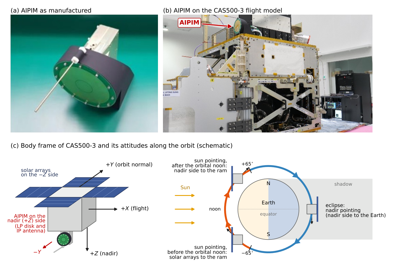
Figure 2.
Operation phases and daily data availability of IAMMAP: S-band science data per sensor and ancillary data (ANC), December 2025–June 2026; the numbers give the days with data.
Figure 2.
Operation phases and daily data availability of IAMMAP: S-band science data per sensor and ancillary data (ANC), December 2025–June 2026; the numbers give the days with data.
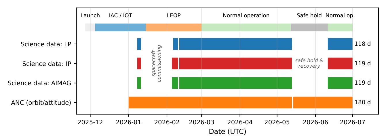
Figure 3.
LP sweeps and fits on 7 February 2026 for a dayside (a–c; 19:18:16 UT, ) and a nightside sweep (d–f; 23:16:42 UT, ): (a,d) TIA output (inverted) with the sweep voltage (thin line); (b,e) up-leg and (c,f) down-leg with (dots), (crosses), the retarding and saturation lines (red, black), and and (dashed); the five lowest-voltage points of each leg are not shown.
Figure 3.
LP sweeps and fits on 7 February 2026 for a dayside (a–c; 19:18:16 UT, ) and a nightside sweep (d–f; 23:16:42 UT, ): (a,d) TIA output (inverted) with the sweep voltage (thin line); (b,e) up-leg and (c,f) down-leg with (dots), (crosses), the retarding and saturation lines (red, black), and and (dashed); the five lowest-voltage points of each leg are not shown.
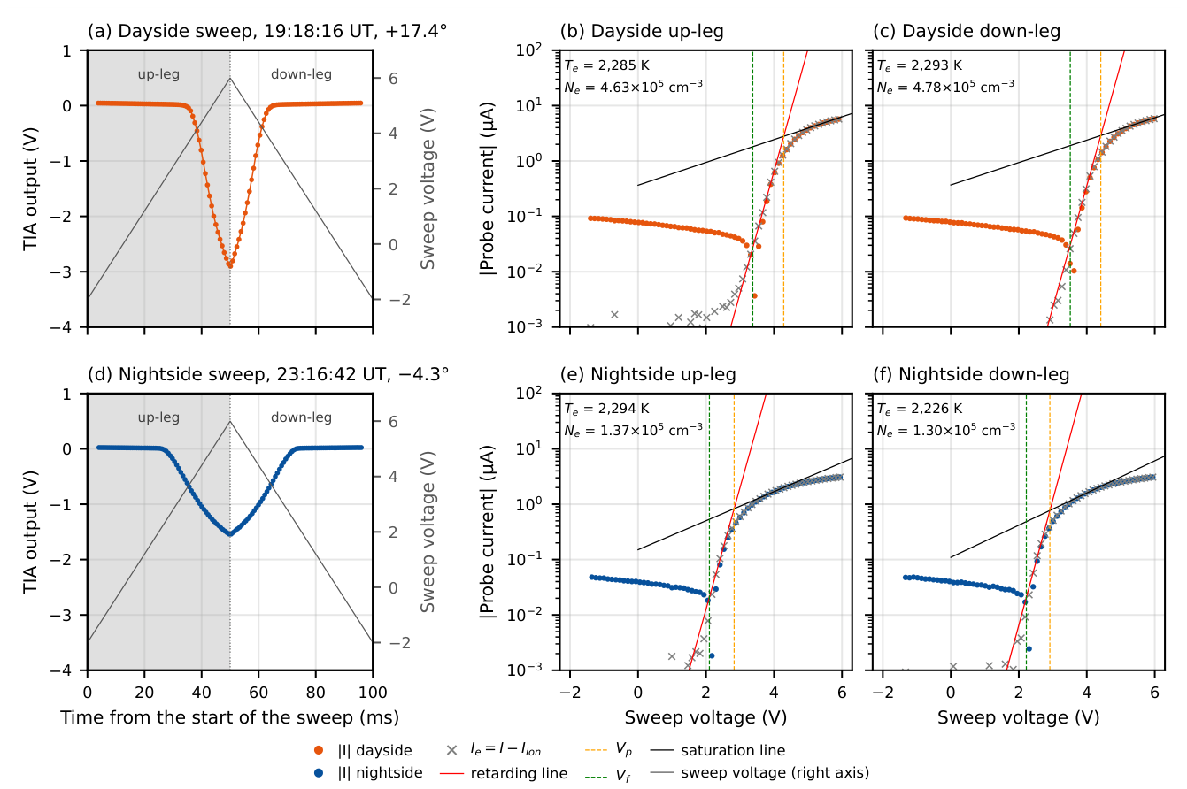
Figure 4.
Up-leg versus down-leg results on the dayside (a–c) and nightside (d–f) of the two reference days: LP (a,d), LP (b,e), and IP (c,f), with the median down-to-up ratio and its scatter (normalized median absolute deviation, in percent).
Figure 4.
Up-leg versus down-leg results on the dayside (a–c) and nightside (d–f) of the two reference days: LP (a,d), LP (b,e), and IP (c,f), with the median down-to-up ratio and its scatter (normalized median absolute deviation, in percent).
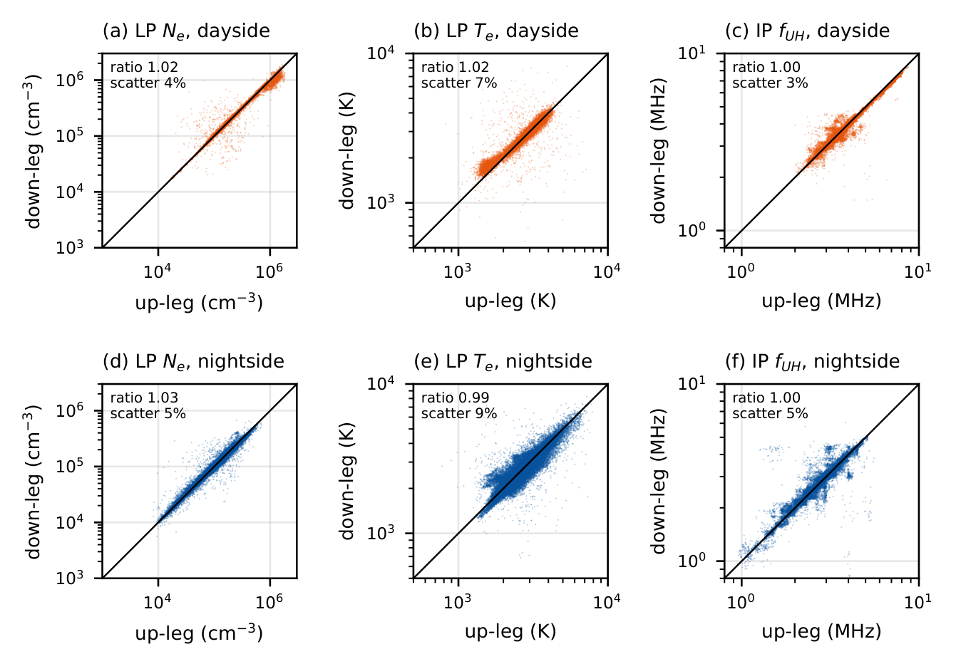
Figure 5.
IP sweeps on 21 June 2026 for a dayside (a–c; 04:24:20 UT, 0.1–10 MHz) and a nightside packet (d–f; 08:20:36 UT, 0.1–5 MHz): (a,d) bridge output with the sweep frequency (thin line); (b,e) up-leg and (c,f) down-leg with the polynomial curve used only to detect the dip (gray), the Savitzky–Golay curve from which is read (black), and (dashed).
Figure 5.
IP sweeps on 21 June 2026 for a dayside (a–c; 04:24:20 UT, 0.1–10 MHz) and a nightside packet (d–f; 08:20:36 UT, 0.1–5 MHz): (a,d) bridge output with the sweep frequency (thin line); (b,e) up-leg and (c,f) down-leg with the polynomial curve used only to detect the dip (gray), the Savitzky–Golay curve from which is read (black), and (dashed).
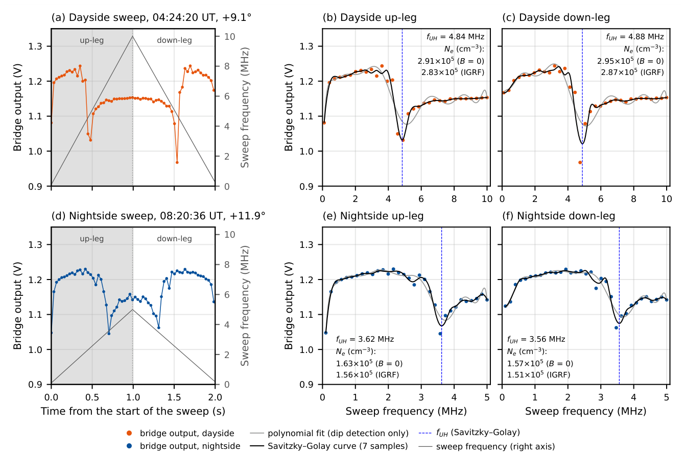
Figure 6.
Electron density of every up-leg on (a) 7 February and (b) 21 June 2026: LP (black) and IGRF-corrected IP (red), with the latitude (thin line) and the operational dayside (orange) and nightside (blue).
Figure 6.
Electron density of every up-leg on (a) 7 February and (b) 21 June 2026: LP (black) and IGRF-corrected IP (red), with the latitude (thin line) and the operational dayside (orange) and nightside (blue).
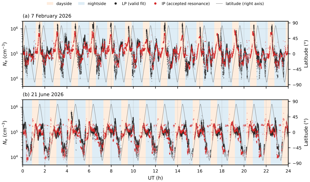
Figure 7.
LP (black) and IP (red) densities against latitude on the dayside (a,c) and the descending nightside pass (b,d) of 7 February (a,b) and 21 June 2026 (c,d): up-legs (dots) and medians in 2° bins (lines).
Figure 7.
LP (black) and IP (red) densities against latitude on the dayside (a,c) and the descending nightside pass (b,d) of 7 February (a,b) and 21 June 2026 (c,d): up-legs (dots) and medians in 2° bins (lines).
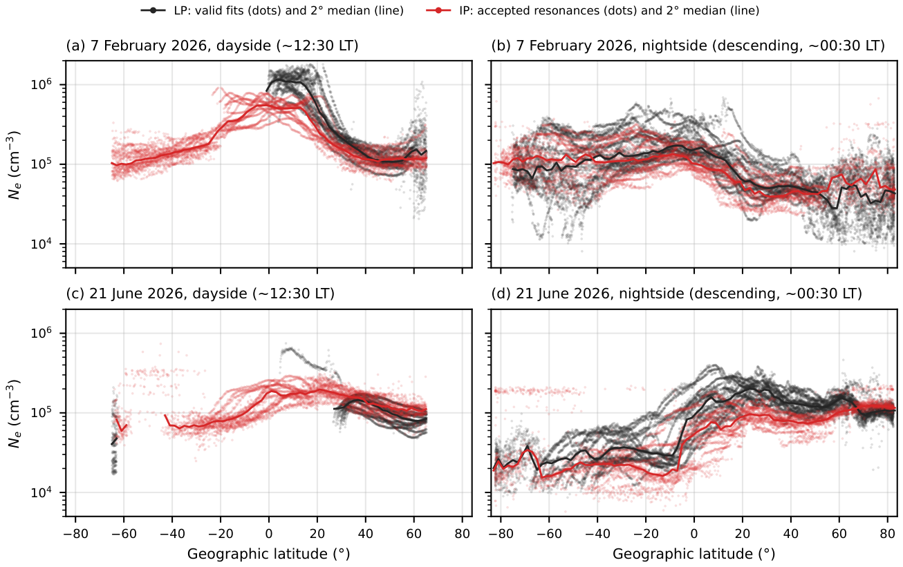
Figure 8.
(a) Peak-to-peak LP amplitude on 21 June 2026 (dayside orange, nightside blue; black: ion-only dayside sweeps below 100 mV). (b) Conceptual I–V curves with of 4, 6, and 10 V within the fixed sweep range (gray). (c) Up-legs at the onset of an ion-only interval on 21 June (04:29:30–04:30:26 UT) with . (d) Fraction of ion-only sweeps on 12 days against the time since the eclipse exit and the angle between the solar-array normal and the direction of flight (ram; purple). (e) Median and interquartile range of of the valid fits.
Figure 8.
(a) Peak-to-peak LP amplitude on 21 June 2026 (dayside orange, nightside blue; black: ion-only dayside sweeps below 100 mV). (b) Conceptual I–V curves with of 4, 6, and 10 V within the fixed sweep range (gray). (c) Up-legs at the onset of an ion-only interval on 21 June (04:29:30–04:30:26 UT) with . (d) Fraction of ion-only sweeps on 12 days against the time since the eclipse exit and the angle between the solar-array normal and the direction of flight (ram; purple). (e) Median and interquartile range of of the valid fits.
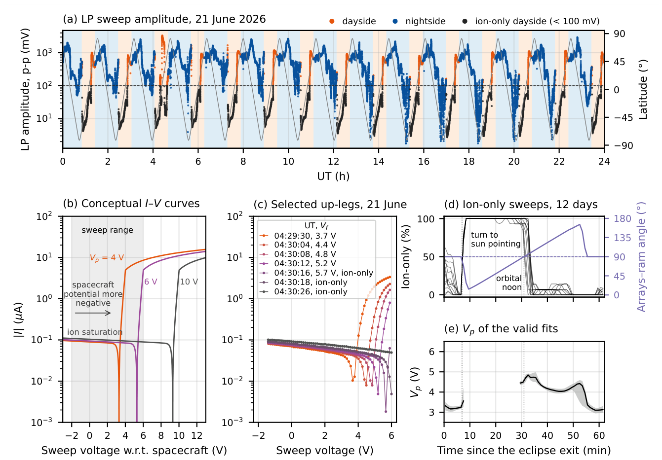
Figure 9.
Fraction of the up-legs with a valid LP fit (filled circles), an ion-only LP sweep (crosses), and an accepted IP resonance (open squares): (a–d) in 5° bins on the dayside and nightside of 7 February and 21 June 2026; (e,f) on the dayside and nightside of 12 days from February to June, with the IP acceptance south of and north of (triangles); shading: safe-hold mode.
Figure 9.
Fraction of the up-legs with a valid LP fit (filled circles), an ion-only LP sweep (crosses), and an accepted IP resonance (open squares): (a–d) in 5° bins on the dayside and nightside of 7 February and 21 June 2026; (e,f) on the dayside and nightside of 12 days from February to June, with the IP acceptance south of and north of (triangles); shading: safe-hold mode.
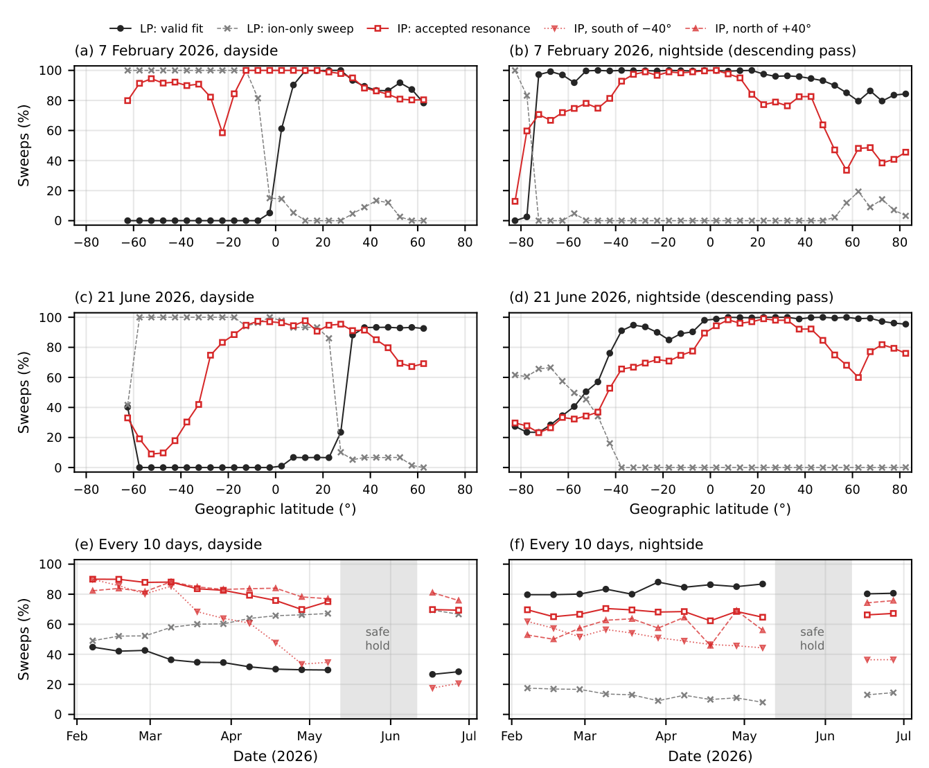
Figure 10.
LP and IP densities of the up-legs in which both probes are valid (dayside orange, nightside blue; circles 7 February, triangles 21 June): (a) IP versus LP density; (b) median and 16–84% range of against ; (c) the same against , and, for comparison, the ratio computed without the field correction (gray).
Figure 10.
LP and IP densities of the up-legs in which both probes are valid (dayside orange, nightside blue; circles 7 February, triangles 21 June): (a) IP versus LP density; (b) median and 16–84% range of against ; (c) the same against , and, for comparison, the ratio computed without the field correction (gray).
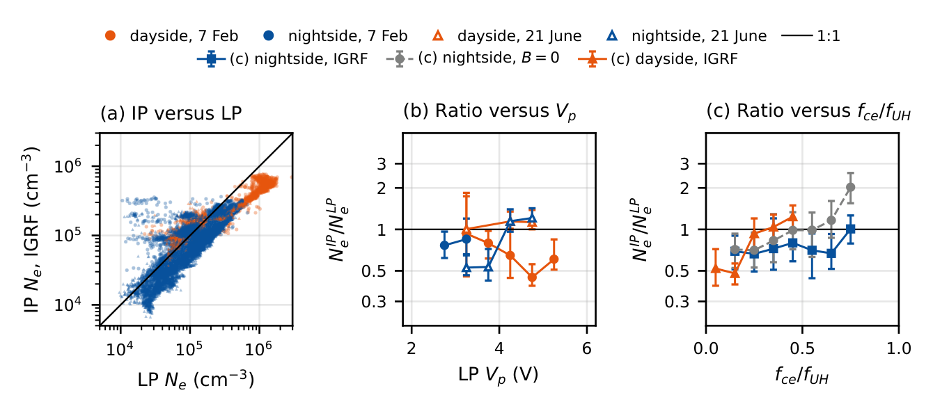
Figure 11.
Ion current of the ion-only LP sweeps of the charged spacecraft as a measure of the density. (a) Three ion-only up-legs of 7 February 2026 (02:47–03:05 UT) with different IP densities: current relative to the start of the fitted range (dots) and fitted line, with its slope s. (b) Slope s against the IP density of the same sweep on the dayside of 7 February (orange circles) and 21 June (purple triangles), with straight-line fits in log–log space (lines), used for Figure 12.
Figure 11.
Ion current of the ion-only LP sweeps of the charged spacecraft as a measure of the density. (a) Three ion-only up-legs of 7 February 2026 (02:47–03:05 UT) with different IP densities: current relative to the start of the fitted range (dots) and fitted line, with its slope s. (b) Slope s against the IP density of the same sweep on the dayside of 7 February (orange circles) and 21 June (purple triangles), with straight-line fits in log–log space (lines), used for Figure 12.
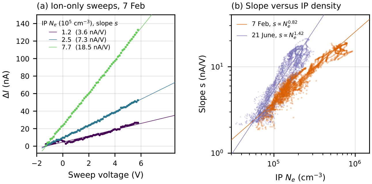
Figure 12.
Electron density along one orbit on (a) 7 February (from 02:04 UT) and (b) 21 June 2026 (from 09:50 UT): LP electron density as fitted (gray) and scaled to the IP (green), density from the ion slope of the ion-only sweeps with the lines of Figure 11b (purple), IP density (red), and the merged profile (black). The brown band shows the full range of the IRI density (PyIRI) along the same track for every day within ±15 days of the same date in 2024–2026. The strip below shows the source of the profile.
Figure 12.
Electron density along one orbit on (a) 7 February (from 02:04 UT) and (b) 21 June 2026 (from 09:50 UT): LP electron density as fitted (gray) and scaled to the IP (green), density from the ion slope of the ion-only sweeps with the lines of Figure 11b (purple), IP density (red), and the merged profile (black). The brown band shows the full range of the IRI density (PyIRI) along the same track for every day within ±15 days of the same date in 2024–2026. The strip below shows the source of the profile.
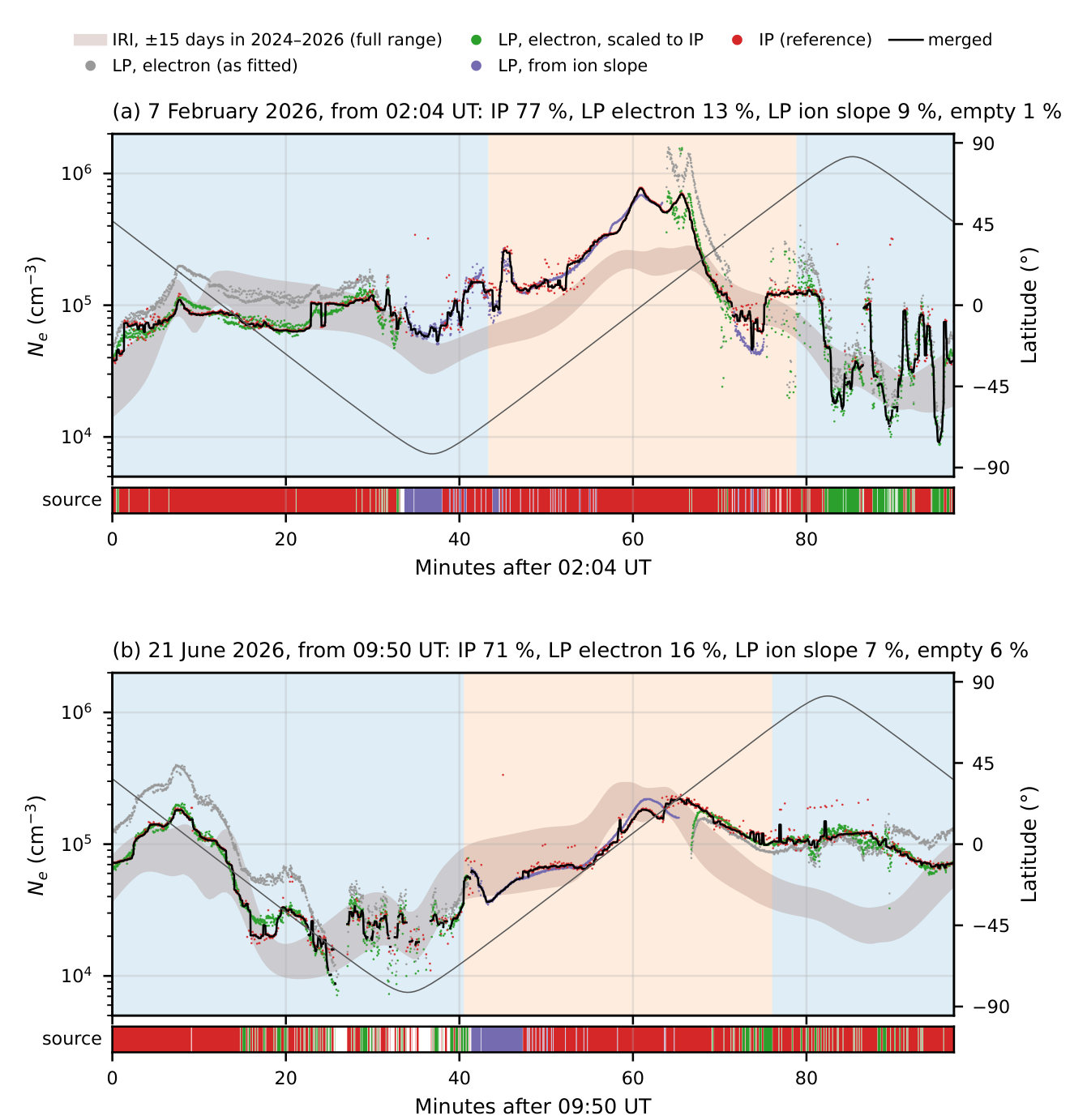

Table 1.
Operational parameters of the plasma probes during the initial-operation period.
| Item | LP | IP |
|---|---|---|
| Sensor | Planar disk, 25.4 mm in diameter, facing sideways () | Short monopole antenna (∼12 cm) along |
| Measured quantity | Probe current through the TIA ( = 500 k) | Capacitance-bridge output vs. frequency |
| Sweep | Triangular, to V with respect to the spacecraft body | 0.1–10 MHz (dayside), 0.1–5 MHz (nightside) |
| Sweep period | 0.1 s (up- and down-leg); the first sweep of every 2 s is transmitted | 2 s per triangular sweep; two sweeps per 4-s packet |
| Sampling | 136 samples per sweep | 31 samples s−1 |
| Derived parameters | , , , ; slope of the ion current (ion-only sweeps) | (with the IGRF field) |
Orbit: Sun-synchronous, ∼600 km, LTAN ≈ 12:30, period ≈ 97 min. IGRF: International Geomagnetic Reference Field.
Table 2.
Up-leg parameters of the sweeps in Figure 3b,e and of two sweeps of 21 June 2026 ( and with respect to the spacecraft body).
Table 2.
Up-leg parameters of the sweeps in Figure 3b,e and of two sweeps of 21 June 2026 ( and with respect to the spacecraft body).
| Date, time (UT) | Region, lat. | (V) | (V) | (K) | (cm−3) | GoF |
|---|---|---|---|---|---|---|
| 2026-02-07 19:18:16 | dayside, | 3.38 | 4.29 | 2,285 | 0.993 | |
| 2026-02-07 23:16:42 | nightside, | 2.10 | 2.83 | 2,294† | 0.985 | |
| 2026-06-21 04:25:56 | dayside, | 3.56 | 4.26 | 1,768 | 0.993 | |
| 2026-06-21 18:00:38 | nightside, | 2.79 | 3.54 | 2,455† | 0.981 |
† Upper limit; see the text.
Table 3.
IP up-legs at the times of the LP sweeps of Table 2: and in MHz, and (with the IGRF field) and in .
Table 3.
IP up-legs at the times of the LP sweeps of Table 2: and in MHz, and (with the IGRF field) and in .
| Date, time (UT) | Region | IP/LP | ||||
|---|---|---|---|---|---|---|
| 2026-02-07 19:18:16 | dayside | 4.40 | 0.80 | 2.32 | 4.63 | 0.50 |
| 2026-02-07 23:16:42 | nightside† | 2.86 | 0.66 | 0.96 | 1.37 | 0.70 |
| 2026-06-21 04:25:56 | dayside | 4.44 | 0.85 | 2.36 | 4.15 | 0.57 |
| 2026-06-21 18:00:38 | nightside | 2.11 | 0.89 | 0.46 | 0.87 | 0.53 |
† Swept over 0.1–10 MHz.
Disclaimer/Publisher’s Note: The statements, opinions and data contained in all publications are solely those of the individual author(s) and contributor(s) and not of MDPI and/or the editor(s). MDPI and/or the editor(s) disclaim responsibility for any injury to people or property resulting from any ideas, methods, instructions or products referred to in the content. |
© 2026 by the authors. Licensee MDPI, Basel, Switzerland. This article is an open access article distributed under the terms and conditions of the Creative Commons Attribution (CC BY) license.
Copyright: This open access article is published under a Creative Commons CC BY 4.0 license, which permit the free download, distribution, and reuse, provided that the author and preprint are cited in any reuse.