

Submitted:
02 November 2026
Posted:
04 November 2026
You are already at the latest version
Abstract
Connectivity laws conserved across systems, independently of edge weights, are compelling in network science. Many network metrics aggregate information counting all shortest-paths between node pairs, which is costly. Here we formalize the all-pairs shortest-path number (APSPN) problem and establish a shared computational foundation for these kinds of problems, including betweenness centrality (BC) and geometrical congruence (GC). We introduce the CC-APSPN kernel, which exploits network science principles to accelerate their shared computations on unweighted graphs via knowledge memoization, reducing runtime by up to 90% over the Brandes-APSPN baseline across diverse network topologies. Parallel CC-APSPN carries this acceleration onto multicore CPUs through batched source processing with a dedicated scheduling strategy, reducing exact BC and GC runtimes from hours to a few minutes on a 100,000-node network. Besides, we propose CC-bbBFS, a single-pair primitive for efficient sampling-based approximation of BC and GC. Together, these advances translate network-science-informed algorithm design into practical large-scale analysis.
Keywords:
shortest-paths count
; network science
; betweenness centrality
; geometrical congruence
; breadth-first search
An enduring goal of network science is to identify principles of connectivity that generalize across systems and scales. For many questions, this means characterizing connectivity through network topology alone, beyond system-specific edge weights or directions1–4. Hence, unless otherwise specified, in this study we intend all networks and the operations defined on them as unweighted and undirected. Shortest paths underpin our understanding of information flow, robustness, and structural organization in complex networks across disciplines ranging from neuroscience to social science and infrastructure analysis5–7. While the all-pairs shortest path (APSP) problem—finding a single shortest path for every node pair—has been extensively studied, some network analyses require information about the number of shortest paths between node pairs. Despite its importance, computing this complete shortest-path information remains challenging.
A diverse set of network metrics shares this dependence. Betweenness centrality (BC)8–10 measures node importance by the fraction of shortest paths through each node or edge and is widely used to identify influential proteins in biological interactomes11, critical nodes in Internet and infrastructure topologies12, and key mediators in communication networks5. Geometrical congruence (GC)13 evaluates the extent to which a network’s topology aligns with its latent geometric space, with applications in brain connectomes and Internet topology where shortest paths align with hyperbolic geodesics6,7,14. Other metrics—including all-pairs shortest-lightest path (APSLP)15 and path hesitation degree (PHD)16—similarly depend on information about all shortest paths. The cost of obtaining this information remains prohibitive for large-scale networks, since the number of shortest paths between node pairs can grow combinatorially with network size and varies strongly across topologies16,17. However, many real-world systems, including social and biological networks, are predominantly scale-free and hierarchically organized6,18–20. This organization increases shortest-path counts but, as we show, allows shortest-path information to be reused across searches. Altogether, these observations motivate network-science-informed algorithm design: using network structure to guide the order of searches and the reuse of their results. Using network science principles for designing memoization and prioritization schemes in algorithms for shortest-path search has already accelerated depth-first search (DFS-based) all-paths enumeration in the Cannistraci-Muscoloni GC algorithm (CM-GC)13 and breadth-first search (BFS-based) single-path search in the Cannistraci-Chen algorithm (CC-BFS)21. Here we extend and elaborate this design principle to accelerate the shared computations underlying a broad class of network metrics in which enumeration and detection of the number of shortest paths between two nodes is crucial.
We formalize this shared dependence as the all-pairs shortest path number (APSPN) problem: given a graph , compute the number of shortest paths for all pairs . We identify BC, GC, APSLP, PHD and related metrics as APSPN-based problems, computed from all-source shortest-path directed acyclic graph (SP-DAG) information and the original input, including auxiliary data, through polynomial-time processing. These problems are equivalent under polynomial-time Turing reductions. Their shared SP-DAG structure provides a constructive basis for universal APSPN kernels, which combine common path-counting techniques with problem-specific accumulation. The natural baseline for such a kernel comes from Brandes’ BC algorithm8, whose path-counting subroutine (here referred to as Brandes-APSPN) performs a single-source search from each node with overall time complexity , where and denote the number of nodes and edges. We generalize Brandes-APSPN into the Brandes-APSPN kernel by adapting its accumulation rules to solve APSPN, BC, GC, APSLP and PHD, while retaining the favorable time for each problem. This generalization allows shared computation improvements to benefit multiple metrics, providing the foundation for our network-science-informed acceleration.
However, the Brandes-APSPN kernel repeats work across sources and becomes too slow for large networks. To overcome this baseline, we introduce the Cannistraci-Chen APSPN (CC-APSPN) kernel, an APSPN kernel that reduced runtime by approximately 30–90% relative to the Brandes-APSPN kernel on large scale-free networks through four network-science-informed schemes: (1) centrality-driven prioritization, (2) all-paths memoization, (3) direction-adaptive propagation, and (4) symmetric mapping. These mechanisms exploit the hierarchical structures of real-world networks and yield the largest gains on scale-free and dense topologies, while preserving the worst-case bound for the five studied problems (APSPN, BC, GC, APSLP, PHD). The kernel also integrates with graph manipulation heuristics for additional speedups. To carry this acceleration onto multicore hardware, we further develop a shared-memory parallel CC-APSPN kernel, which preserves cross-source memoization through batched source processing and introduces, for BC, a novel cross-batch pipeline that overlaps one batch’s dependency accumulation with the next batch’s path counting. Compared with the sequential Brandes-APSPN kernel, parallel CC-APSPN reduced exact BC and GC runtimes on a 100,000-node scale-free network from hours to minutes, and a similar advantage was observed on real-world networks.
For networks where even an accelerated exact computation is infeasible, we develop a complementary sampling-based approximation route. Cannistraci-Chen balanced bidirectional breadth-first search (CC-bbBFS) is a shared single-pair primitive that supplies the exact per-pair contributions required by BC and GC. Built on it, CC-ApproxBC achieves, in general, both higher efficiency and accuracy than SILVAN22 and KADABRA23 (previous state-of-the-art approximate BC algorithms). CC-ApproxGC is, to our knowledge, the first sampling-based GC algorithm with a practical stopping rule that enables highly efficient GC approximation.
Together, the shared kernel CC-APSPN and the single-pair primitive CC-bbBFS extend network-science-informed design of shortest path count across network metrics to exact and approximate computation respectively.
Results
A unified framework for APSPN-based problems
While the all-pairs shortest path (APSP) problem measures the shortest path length between each node pair, many key network analyses require enumerating or counting all shortest paths between node pairs6,8,13. A subcubic equivalence between BC and APSP has been established for the unique-shortest-path formulation using randomized reductions with high success probability24. Yet the literature has addressed enumeration only implicitly, as a subroutine for metrics such as BC or stress centrality25, under fragmented terminology including #APSP26 and all-pairs all shortest path (APASP)27.
To resolve this fragmentation, we formalize the all-pairs shortest path number (APSPN) problem: given a graph where and respectively denote the set of nodes and edges, compute the number of shortest paths for all pairs . APSPN generalizes APSP (Fig. 1a) and underlies several network metrics: BC requires , the fraction of shortest – paths through node ; GC, as formalized by Cannistraci and Muscoloni13, compares the geometric projection of topological shortest paths with geodesics in latent geometric space; all-pairs shortest-lightest path (APSLP)15, BC variants such as stress centrality, and path hesitation degree (PHD)16 similarly depend on APSPN.
The common substrate of these problems is the definition of a specific data structure called shortest path directed acyclic graph (SP-DAG)8. For a source node , its SP-DAG () is the minimal subgraph containing all shortest paths from , and solving the single-source shortest path number (SSSPN) problem amounts to traversing and accumulating path counts in topological order. For APSP, a shortest-path tree retains one representative path to each reachable node and suffices to recover distances. For APSPN, the SP-DAG additionally preserves alternative shortest paths, enabling path counting without explicitly enumerating them (Fig. 1a). The union of all SP-DAGs forms the network’s metric backbone28,29.
We define APSPN-based problems as problems computable from all-source SP-DAG information and the original input, including auxiliary numerical data, through a polynomial number of complete SP-DAG traversals with polynomial-time processing. This class includes APSPN, BC, GC, APSLP, PHD, and related metrics. All APSPN-based problems are polynomial-time Turing equivalent under the computational model of Supplementary Theorem 1. Their shared SP-DAG computations provide a constructive basis for universal APSPN kernels.
The Brandes-APSPN kernel as baseline
Traditionally, BC was computed by summing the fraction of shortest paths through each node over all source-target pairs after solving APSPN, which is . Brandes’ BC algorithm8 reduced this to (where and denote the number of edges and nodes, respectively) by exploiting the SP-DAGs, and remains the state of the art. We refer to its path-counting subroutine as the Brandes-APSPN, the foundation for all subsequent APSPN-based computations.
Brandes-APSPN performs an independent single-source search (breadth-first-search, BFS, in per source), constructing the SP-DAG and accumulating path counts from predecessors:
where is the set of predecessors of in and is the number of shortest paths from to . Repeating across all sources yields the APSPN matrix in time.
We generalize Brandes-APSPN into the Brandes-APSPN kernel by adapting its accumulation logic to the other studied problems (GC, BC, APSLP and PHD), each preserving the bound. However, an important limitation of Brandes-APSPN is that its independent per-source searches duplicate work on large dense or scale-free networks, where redundant traversal dominates runtime. In the next section, we will discuss how network science principles can inform design of algorithms to address this limitation.
A network-science-informed CC-APSPN kernel
We introduce the CC-APSPN kernel, a network-science-informed APSPN kernel that achieves order-of-magnitude empirical speedups over the Brandes-APSPN kernel while preserving its worst-case complexity for the five mentioned problems (APSPN, GC, BC, APSLP and PHD, Supplementary Note 3). Here and denote the numbers of nodes and edges, respectively. Precomputed APSP distances and source node prioritization guide CC-APSPN kernel’s single-source searches (Fig. 1c). The kernel combines four network-science principles (Fig. 1d–f): (i) centrality-driven prioritization (Pri, Fig. 1d left) processes sources in descending degree order so that influential hubs in scale-free networks are processed first, making their path information available to later searches; (ii) all-paths memoization (Mem, Fig. 1d right) reuses path counts from previously processed neighbors, avoiding rediscovery of paths through hubs; (iii) direction-adaptive propagation (DAP, Fig. 1e) chooses between forward and backward propagation across consecutive shortest-path levels based on edge traversal cost, yielding substantial savings under heterogeneous level node distributions; and (iv) symmetric mapping (Symm, Fig. 1f) exploits the path symmetry to recover previously computed path counts during backward propagation (where and denote arbitrary source and target nodes, and denotes the number of shortest paths from to ). To balance memoization overhead against saved traversal work, we apply Mem only when the current source has degree at most , where is the average node degree. We derive this threshold from a model of memoization and traversal costs (Supplementary Note 2). The full formulation, including the memoization constraints and propagation cost estimates, is given in the Methods.
The core challenge in dynamic programming is to reuse information across searches while retaining the contributions of all shortest paths. CC-APSPN addresses this by adapting principles from CM-GC13 and CC-BFS21 to path counting (Fig. 1b), with Symm providing additional reuse through path symmetry. The empirical advantage is most pronounced on heterogeneous, hierarchical topologies such as scale-free networks, where path reuse yields substantial reductions in computation; on homogeneous topologies, the gains can narrow or even disappear. Adapting the CC-APSPN kernel to any other APSPN-based problem requires only modifying the accumulation logic (see Methods).
Combining CC-APSPN with graph manipulation heuristics
Existing strategies for accelerating BC fall into three categories: approximation by sampling30–32, which trades exactness for speed; parallelization33, which reduces wall-clock time but not total work; and graph manipulation34–41, which compresses the input without sacrificing exactness.
Puzis et al.34,35 show that two graph-manipulation heuristics, biconnected components decomposition (BCC) and structural equivalence (SE), are particularly effective for BC and therefore for APSPN-based problems. BCC decomposes the graph along articulation points, allowing independent computation on smaller subgraphs; SE merges nodes with identical neighborhoods—which share identical BC contributions—into super-nodes (Fig. 1g). Neither improves the worst-case bound.
Because graph manipulation is orthogonal to kernel choice, we combine the two heuristics with the CC-APSPN kernel following the multi-stage pipeline of Puzis et al.34,35 (Fig. 1g): we apply the heuristics sequentially, invoke the CC-APSPN kernel on the maximally compressed graph—whose raised heterogeneity further amplifies the kernel’s advantage—and reconstruct exact results for the original graph in postprocessing (see Methods). For problems which integrate the shortest path count on the topology with other information, namely GC (reference distances) and APSLP (edge weights), only BCC is applicable, since SE would discard this information.
Benchmarking APSPN kernels across artificial and real-world network topologies
To test how network-science-informed design translates into practical speedups, we benchmarked the sequential CC-APSPN kernel against the Brandes-APSPN kernel across all five studied APSPN-based problems (of which the results of APSPN, BC and GC are extensively discussed here), and against the specialized CM-GC algorithm for GC. We used three complementary testbeds: artificial networks generated by the nonuniform popularity-similarity optimization (nPSO)42 model, Watts–Strogatz (WS) networks1, and real-world networks from the ATLAS dataset21. The nPSO model captures the hyperbolic scale-free topology with average node clustering and community organization typical of real-world complex networks6,18–20,43; WS provides a controlled non-scale-free contrast with different levels of average node clustering; the whole ATLAS dataset comprises 1,842 real-world networks across 35 classes, making it a stringent benchmark with broad topological diversity.
An ablation test supported the combined design: the full kernel performed best or comparably to the fastest ablated variant across the tested settings (Extended Data Fig. 2).
On nPSO networks, the CC-APSPN kernel consistently outperformed the Brandes-APSPN kernel, and the gap widened with size and density, reaching approximately a runtime reduction on dense networks of nodes (Fig. 2). Sweeping topological parameters at (power-law exponent , temperature (clustering), and number of communities), the kernel retained a substantial advantage at both high (, Fig. 3) and low (, Extended Data Fig. 3) densities, achieving speedups of 3.9–18.0× over the Brandes-APSPN kernel on dense networks. This advantage extended across all five studied problems (Extended Data Fig. 1, 10,000-node nPSO). In particular, CC-APSPN outperformed the Brandes-APSPN kernel in all 24 tested configurations, achieving speedups of 1.7–5.8× for APSLP (Extended Data Fig. 1d,i,n) and 1.6–5.3× for PHD (Extended Data Fig. 1e,j,o). Compared with the former GC baseline, CM-GC, which often failed to complete within reasonable time, the CC-APSPN kernel outperformed it by a factor of 6.7–602 (Extended Data Fig. 1b,g,l).
On Watts–Strogatz networks, the sequential advantage was smaller (Extended Data Fig. 4, 10,000 nodes) but still reached 5.9× for BC in the dense and low-clustering case (, Extended Data Fig. 4h). CC-APSPN was slower than Brandes-APSPN in some sparse, high-clustering and homogeneous degree cases (, Extended Data Fig. 4a,c,d), but faster in most other settings. An explanation is that at there is no rewiring, all nodes have the same degree, and equal degrees eliminate the structural hierarchy from which memoization benefits, while inexpensive sparse traversals leave less computation to save relative to bookkeeping overhead. Parallel CC-APSPN was fastest throughout.
On all 457 ATLAS networks tested, the sequential CC-APSPN kernel was substantially faster (1.76–5.65×) than the Brandes-APSPN kernel (Fig. 4g,h). Combining the kernel with graph manipulation heuristics further increased the advantage. Among the ten networks with the largest gains, SE+BCC gave the highest mean speedup, 5.71× (Fig. 5b), with the largest individual gains occurring mainly on social networks (Fig. 5a).
Parallel CC-APSPN kernel scales across CPU threads
To carry the principled optimizations onto multicore CPUs, we retain the degree-prioritized source order and advance in synchronized batches of at most one source per thread. Searches within a batch run concurrently and reuse results only from completed earlier batches.
For BC, path counts are ready for memoization before their source’s backward dependency accumulation finishes. We exploit this separation with a cross-batch pipeline: dependency tasks from one batch share a worker queue with path-counting tasks from the next. Workers finishing dependency tasks can begin the next searches while slower dependency tasks continue.
This adds thread-level acceleration to the sequential kernel’s savings. Relative to sequential CC-APSPN, parallel CC-APSPN at 32 threads achieved speedups of 10.2–19.0× for APSPN, 12.6–20.7× for BC and 9.5–17.7× for GC across the tested network topologies (Figs. 2 and 3, Extended Data Fig. 3). For BC on the ATLAS networks, the speedups ranged from 8.1× to 31.2× (Fig. 4a–f). As an example, on the dense 100,000-node nPSO network with 1% edge density, BC computation fell from 15.0 h with sequential Brandes-APSPN to 4.7 min with parallel CC-APSPN (Fig. 2e).
The parallel CC-APSPN kernel showed substantial gains up to 16 threads on both testbeds, with smaller additional gains at 32. Across nine 10,000-node nPSO configurations, 32-thread mean speedups over sequential Brandes-APSPN reached 77.5× for parallel CC-APSPN, 9.9× for parallel Brandes-APSPN and 5.3× for NetworKit’s parallel Brandes’ BC implementation44 (Extended Data Fig. 5). NetworKit is a popular open-source toolkit for large-scale network analysis.
On ATLAS networks with 5,000–100,000 nodes, CC-APSPN’s mean speedup increased from 55.3× at 16 threads to 63.7× at 32, whereas Parallel Brandes-APSPN and NetworKit plateaued after 16 threads, reaching mean speedups of 8.5× and 7.2× at 32, respectively (Extended Data Fig. 6a). At 32 threads, CC-APSPN was faster than these competitors by a median of 7.80× and 9.27×, respectively (Extended Data Fig. 6b).
CC-bbBFS enables efficient node-pair sampling
Even with an efficient APSPN kernel, the worst-case cost of exact computation limits its reach on the largest networks. Sampling offers a complementary route: BC and GC can be estimated from a small sample of node pairs, provided each search returns the shortest-path contributions required by the metric (Fig. 6a). We therefore propose CC-bbBFS, a single-pair primitive shared by the BC and GC approximation algorithms that supplies, for any sampled pair , the distance , the shortest-path number , the per-node path counts required by BC (with an intermediate node), and the projection sums over topological shortest paths required by GC.
CC-bbBFS is based on the balanced bidirectional BFS (bbBFS) of Borassi and Natale23. Starting from both endpoints, it advances the frontier with the smaller estimated traversal cost based on frontier degrees, and aggregates path counts across the edges where the two frontiers meet (Fig. 6b). We observed that, in ultra-small-world networks (networks with nodes, whose average shortest path length scales as , produced by the nPSO model), sampled pairs are dominated by very short geodesics; CC-bbBFS therefore short-circuits distance-one and distance-two pairs to avoid a full bidirectional expansion.
Here, memoization is organized around recurring endpoints rather than a prioritized source sequence. CC-bbBFS memoizes depth-limited search states for each endpoint up to , where is the number of nodes and is the average node degree (Fig. 6c). This rule controls state-management overhead while allowing deeper reuse as network size and connectivity increase (Methods). Revisiting an endpoint replays stored levels before resuming exploration, thereby avoiding repeated traversal.
Faster and more accurate BC approximation with CC-ApproxBC
We use CC-bbBFS to accelerate BC approximation. CC-ApproxBC retains the progressive-sampling strategy of SILVAN22, the state-of-the-art approximate-BC algorithm, but replaces its bbBFS step with CC-bbBFS, which directly returns exact per-pair dependencies and removes the additional path-sampling step on the single-pair shortest-path directed acyclic graph (SPSP-DAG, Fig. 6b). We benchmarked CC-ApproxBC against SILVAN and KADABRA23 (another established approximate-BC algorithm) on 343 real-world ATLAS networks (Fig. 6d), the SILVAN benchmark dataset (Fig. 6e; 15 networks up to 2.4 million nodes), and nPSO networks (Fig. 6f), with identical approximation parameters. For each method we report runtime and errors in the normalized BC : the maximum absolute error , and the mean relative absolute error MRAE over nodes with nonzero exact BC (Methods).
Across all three datasets, CC-ApproxBC was the fastest method, with the best or competitive accuracy in MAE and MRAE. On ATLAS, CC-ApproxBC reduced mean runtime from 69.4 s with SILVAN and 13.0 s with KADABRA to 9.9 s, while cutting average MAE by approximately 43% relative to either competitor (Fig. 6d). The advantage over SILVAN was largest here, where high shortest-path counts inflate SILVAN’s path-sampling cost, making these networks particularly well suited to computing per-pair contributions directly. On the SILVAN benchmark, CC-ApproxBC averaged 12.3 s versus 25.1 s for SILVAN and 49.6 s for KADABRA, with average MAE reductions of 33% and 23%, respectively (Fig. 6e). On nPSO networks, CC-ApproxBC averaged 3.0 s versus 4.7 s and 3.6 s, respectively, and achieved the lowest average MRAE (0.57 versus 0.64 and 1.36; Fig. 6f). Overall, KADABRA retained a competitive error–time balance despite using less per-pair information.
Sampling-controlled GC approximation with CC-ApproxGC
Unlike BC, network geometrical congruence (GC) has no established sampling algorithm with a practical stopping rule. CC-ApproxGC addresses this by sampling non-adjacent node pairs and using CC-bbBFS to compute the exact GC contribution of each sampled pair. The number of samples is controlled by a single sampling factor (), with sampled pairs for a network of nodes, allowing users to control the tradeoff between runtime and approximation error.
On ATLAS networks, increasing the sampling factor from 0.1 to 15 reduced mean relative error from 0.42% to 0.035%, while mean runtime increased from 7.0 s to 51.7 s (Fig. 6g). On nPSO networks, the same increase reduced mean relative error from 0.29% to 0.023%, while mean runtime increased from 0.82 s to 8.6 s (Fig. 6h). The fitted exponents were consistent with inverse-square-root error scaling (Extended Data Figs. 7 and 8). The error–runtime cost (the product of mean runtime and mean absolute error each normalized by its minimum across sampling factors) was lowest at for ATLAS and for nPSO (Fig. 6i). Across the evaluated datasets, sampling factors between 1 and 5 provide a practical balance between approximation accuracy and computational cost, with the preferred setting depending on network structure.
Discussion
Our results demonstrate that network-science-informed algorithm design for the all-pairs shortest-path number (APSPN) problem can substantially accelerate the computation of four distinct measures in complex network analysis. Their common SP-DAG structure provides a basis for universal kernels, allowing topology-guided reuse to accelerate BC, GC, APSLP and PHD together by pairing shared path counting with problem-specific accumulation. On dense scale-free networks with 100,000 nodes, the CC-APSPN kernel reduced BC and GC runtimes by approximately 90% relative to Brandes-APSPN. The same kernel achieved speedups of 1.7–5.8× for APSLP and 1.6–5.3× for PHD, demonstrating that this shared acceleration also benefits distinct tasks such as selecting the lightest shortest paths and quantifying shortest-path multiplicity. Parallel processing and CC-bbBFS extend the reach of this approach to multicore execution and sampling-based approximation.
The resulting computational savings expand the scale of BC and GC analyses, from whole-brain connectomes45 and Internet autonomous-system networks (tens of thousands of nodes) to much larger social networks (millions to hundreds of millions of nodes), supporting future applications in network dismantling46,47, super-spreader identification48, mapping of central regulatory proteins11, and information-flow optimization49.
The progression from previous studies such as CM-GC13 and CC-BFS21 to the present work illustrates a transferable design principle: “let network structural features guide what to compute first, what to retain and where to reuse it”. In CC-APSPN, degree-prioritized sources make reusable path information available early; in CC-bbBFS, short geodesics motivate targeted shortcuts, while repeated endpoints permit memoized search states to be replayed. This connection between topology and information reuse offers a dynamic programming basis for accelerating other graph computations dominated by repeated traversal.
The benefits of memoization depend on the balance between reuse and the cost of managing stored information. As our ablations indicate, without constraint, state-management overhead can eventually outweigh the traversal work saved. In each of our algorithms, we therefore limit memoization using a constraint suited to the problem: the degree threshold in the CC-APSPN kernel and the depth limit in CC-bbBFS; the hub-set and vector-comparison constraints previously introduced in CC-BFS21 play an analogous role. Here is the number of nodes and the average node degree.
The present work also has limitations. First, the empirical gains depend on network degree heterogeneity—on sparse networks with homogeneous node degrees the benefit can diminish. However, such networks are rare in real scenarios as demonstrated by the results on the 457 real networks in the ATLAS. Finally, although our sequential speedups can go from roughly 1.8–5.6× on real networks, both kernels retain the time bound for the five studied problems; improving this bound remains an open challenge.
Several directions naturally extend this work. Our next step is a distributed-memory implementation of the CC-APSPN kernel for supercomputers, which would remove the runtime and memory limits of a single machine. With it, we aim to compute exact BC and GC on the largest networks for which these measures have ever been computed. GPU-based implementations and extensions to dynamic or streaming networks are further directions. The framework accommodates new metrics whose SP-DAG traversals, auxiliary-data processing and output generation satisfy the same polynomial-time conditions.
Methods
Shortest paths and the SP-DAG
Let be a graph with node set , edge set , and a positive edge-weight function ; we assume has no self-loops or multiple edges, and write and . A path from a source to a target is a sequence of nodes with , , and for ; its length is . A path is a shortest path (SP) if is minimal among all - paths, in which case we write the shortest-path distance as . For unweighted graphs, for all . Throughout the article, a double-subscript (or ) denotes an edge weight, whereas a single-subscript denotes the degree of node , with the average node degree.
We denote the set of all shortest paths from to by and its size by . For any node , is the subset of shortest paths visiting , with . Extending to subsets of nodes, is the set of shortest paths from to that visit at least one node of .
For any source , the shortest-path directed acyclic graph (SP-DAG), , is the minimal subgraph of containing every shortest path originating at . Its node and edge sets are
Because all edge weights are strictly positive, is a DAG with as its unique source (the only node with no predecessors). Unless stated otherwise, the algorithms and experiments below assume is unweighted and undirected.
APSPN-based problems and APSPN kernels
We define APSPN-based problems as problems computable from all-source SP-DAG information and the original input, including auxiliary numerical data, through a polynomial number of complete SP-DAG traversals with polynomial-time accumulation, postprocessing and output generation. Based on Brandes’ approach8 (see Brandes-APSPN kernel below), APSPN, GC, APSLP, and PHD can be computed with one traversal per source, while BC uses one forward traversal for path counting and one backward traversal for dependency accumulation. All APSPN-based problems are polynomial-time Turing equivalent for both unweighted and strictly positive weighted shortest-path formulations (Supplementary Theorem 1). Polynomial time is measured in total input bit length, including finitely encoded numerical data supporting exact polynomial-time arithmetic and comparison. This equivalence does not imply that one metric’s output determines another’s or that their optimal running times coincide. We refer to the results of solving these problems as APSPN-based metrics (or measures); terminology and notation are summarized in Supplementary Table 1.
Edge weights play two different roles across this problem family, and we distinguish them explicitly to avoid ambiguity. APSP, APSPN, BC, and PHD each come in an unweighted and a weighted version: edge weights enter the path length and thereby determine which paths are shortest, making the two versions genuinely different computational problems (requiring BFS-style and Dijkstra-style searches, respectively). These four problems also admit directed formulations. In this article, we focus on the unweighted versions, in which shortest paths are those with the fewest edges (hops). For GC and APSLP as defined here, shortest paths remain the hop-minimal topological shortest paths (TSPs) of the unweighted topology, and the additional information they consume (reference distances for GC, edge weights for APSLP) serves only to evaluate (GC) or select among (APSLP) the TSPs. Restricting to unweighted graphs therefore entails no loss for GC and APSLP: the versions addressed here are the complete problems.
An APSPN kernel is any algorithm that (1) correctly solves every APSPN-based problem, and (2) when invoked on a given APSPN-based problem, can also output the underlying APSPN matrix within the same asymptotic time complexity. The second requirement ensures that the kernel never sacrifices the fundamental path-counting operation for problem-specific optimization. This article develops two APSPN kernels for unweighted graphs: the Brandes-APSPN kernel, derived from Brandes’ algorithm8, and the CC-APSPN kernel. Their implementations cover APSPN, BC, GC, APSLP and PHD; further problems require their corresponding processing routines.
All-pairs shortest path number (APSPN)
The APSPN problem is to compute the number of shortest paths between every pair of nodes ,
where denotes the set of nodes in the graph and denotes the set of shortest paths from to . By convention for every . In analogy to the single-source shortest path (SSSP) variant of APSP, the single-source shortest path number (SSSPN) problem asks for at a fixed source and all .
Betweenness centrality (BC)
Here, we use BC to refer to node betweenness centrality. The BC score of a node measures its importance as a relay in shortest-path information flow. While its variants exist (such as those based on random walks50), the standard definition, introduced by Freeman5, is
where is the node set, is the number of shortest paths from source to target , and is the number of those shortest paths that pass through node . The sum runs over distinct endpoint pairs, with neither endpoint equal to , counting each unordered pair once for undirected graphs and each ordered pair once for directed graphs; pairs with no connecting path contribute zero. This is the unnormalized BC returned by our implementations.
Network geometrical congruence (GC)
For a graph with node set , edge set , number of nodes , and number of edges , let denote a reference-distance matrix. GC quantifies how well the topological structure of aligns with the latent geometry represented by . Following the definition by Cannistraci and Muscoloni13,
where is the set of unordered non-adjacent node pairs, so that and the prefactor turns the sum into an average. A topological shortest path (TSP) between two nodes is a path with the fewest edges (hops), and its projection is the sum of reference distances over the consecutive node pairs along the path. denotes the mean projection over all TSPs from to ; computing it aggregates contributions over all such paths, which places GC within the APSPN-based problems. The averaging set must be nonempty, and its pairwise GC contributions must be well-defined and finite.
GC is defined on the unweighted and undirected topology. The reference distances typically encode pairwise geodesic distances in the graph’s latent geometric space and must be supplied as input.
For nPSO networks, reference distances are supplied by the model’s native hyperbolic geometry. For ATLAS and WS networks, no latent geometry is supplied, so we derive following the default procedure introduced by Cannistraci and Muscoloni13. We first pre-weight every edge with the repulsion-attraction (RA) rule51, a topology-driven dissimilarity measure that infers edge weights from connectivity alone. We then compute the geometrical shortest path (GSP), the weighted shortest path on the RA-weighted network, between all node pairs and adopt its length as , so that the GSP serves as a topology-derived surrogate for the latent geodesic distance.
All-pairs shortest-lightest path (APSLP)
For an edge-weighted graph , the APSLP problem15 asks to find, for each node pair , a TSP (topological shortest path, defined above) of minimum total edge weight (i.e., the lightest). APSLP selects the lightest among the TSPs between and using minimum-weight accumulation on the SP-DAGs, which places it within the APSPN-based problems. Edge weights serve as a secondary index for path selection; if all edge weights are identical, APSLP reduces to ordinary APSP.
Path hesitation degree (PHD)
The PHD16 of a node is the average number of shortest paths from to all other nodes,
where denotes the number of nodes, denotes the set of nodes, and is the number of shortest paths from node to node . A high indicates that has, on average, many alternative shortest paths to the rest of the network. The PHD problem is to compute for every ; the distribution of pairwise shortest-path counts has been observed to follow a power law in many real-world complex networks16.
CM-GC
The original GC algorithm of Cannistraci and Muscoloni13, hereafter CM-GC, computes the mean projection by explicit path enumeration. From each source node, it performs a recursive depth-first search (DFS) up to a pre-assigned maximum recursion depth, which ensures that every TSP required for that source’s assigned node pairs is traversed exactly once; whenever the current path reaches a node at exactly its shortest-path distance from the source, the path is a TSP, and its projection (the sum of reference distances along its edges) is accumulated. Dividing the accumulated projection by the number of traversed TSPs (which equals , the number of shortest paths from the source to the target ) yields .
CM-GC is the first network-science-informed algorithm for GC that significantly reduced the computational complexity of the naïve brute-force search. It uses two network-science principles to reduce the recursion depths: memoization ensures that the of each unordered node pair is computed only once, so that each source’s maximum recursion depth can be pre-assigned while neglecting all previously processed sources; prioritization orders the sources by decreasing average TSP length to all other nodes, placing nodes that carry many long paths first and thereby maximizing the depth reduction available to later sources.
Since the recursion branches over the neighbors of every visited node, the cost for a source with recursion depth grows approximately as , where is the average node degree. The overall time complexity is then (Extended Data Table 1), where is the number of nodes, is the network diameter, and is the proportion of nodes with recursion depth . This exponential dependence on the recursion depth restricts CM-GC to small-world networks with low diameter; the APSPN kernels introduced in the following subsections avoid the recursion by accumulating projections over the SP-DAGs rather than enumerating individual paths (see “Computing APSPN-based metrics”, below), making GC computable in polynomial time.
Brandes-APSPN kernel
The Brandes-APSPN kernel is our baseline APSPN kernel for unweighted graphs. Its core procedure, Brandes-APSPN, is the same path-counting subroutine of Brandes’ BC algorithm8.
Brandes-APSPN performs an independent single-source search from each source (a BFS for unweighted graphs or Dijkstra’s algorithm for weighted graphs) to count all shortest paths originating at . The traversal naturally constructs the SP-DAG . The number of shortest paths from to any node , , is accumulated from ’s predecessors in as
where is the predecessor set of in , and is the number of shortest paths from to predecessor . Repeating across all sources yields the complete APSPN matrix in time for unweighted graphs.
Detailed pseudocode and line-by-line complexity annotations are provided in Supplementary Algorithm 1. The Brandes-APSPN kernel is the generalization of Brandes-APSPN to other APSPN-based problems via problem-specific modifications (see “Computing APSPN-based metrics”, below). For simplicity, in figures we may omit the word “kernel” from the full algorithm names.
CC-APSPN kernel
The CC-APSPN kernel is a network-science-informed APSPN kernel for unweighted graphs. Unlike the Brandes-APSPN kernel, which computes all shortest paths from scratch for each source, the CC-APSPN kernel guides each search with precomputed pairwise distances and reuses shortest-path information from previously processed sources. We describe its core procedure (CC-APSPN, for APSPN computation) in three steps below (Fig. 1c); for other problems, only minor modifications are required (see the next subsection).
Step 1 — APSP computation and prioritization. The algorithm first computes the APSP distance matrix using CC-BFS21, a network-science-informed dynamic-programming variant of BFS for unweighted APSP. CC-BFS retains the worst-case bound of standard BFS-based APSP, but decomposes the search around a small set of influential hubs and reuses their precomputed shortest-path structures to prune redundant traversal, yielding order-of-magnitude empirical speedups and providing exact distance reference for the CC-APSPN kernel. The kernel then scores each node by a centrality measure (degree centrality as used here) and processes sources in descending order of their centrality scores (i.e., centrality-driven prioritization). This ensures that influential hubs, which tend to lie on many shortest paths, are processed first, so their path information becomes available for reuse in Step 2. Here and denote the numbers of nodes and edges, respectively.
Step 2 — Distance-guided single-source search. For each source in the prioritized list (where denotes the th source node to be processed, and is the number of nodes), the algorithm performs a distance-guided single-source search. First, using the precomputed distances, it partitions nodes reachable from the source into distinct shortest-path levels for , where is the maximum finite distance from , and proceeds level by level from upward. For each target node , the total path count is decomposed as , the sum of a memoized component and a traversal component . The two components are computed by the following three sub-procedures. Here is the set of nodes reachable from the source; unreachable pairs retain zero path counts.
(a) All-paths memoization (Mem). Memoization is condition-based (Fig. 1d) and is applied only when the source has low degree, , where is the degree of source , and is a degree threshold set as in our experiments, with the average node degree (see Supplementary Note 2 for its derivation). Only a previously processed neighbor of qualifies as a memoization source (i.e., where is the neighborhood of ). For each target with , the memoized path count is
Memoization sources used in this step are removed from the frontier to prevent double counting.
(b) Direction-adaptive propagation (DAP). The algorithm computes the traversal component by propagating path counts between consecutive levels and (Fig. 1e). DAP estimates the cost of each direction and proceeds in the cheaper one:
Forward propagation iterates over in the current frontier and updates path counts at their successors in , with cost , where denotes the degree of node .
Backward propagation iterates over and aggregates path counts from its predecessors in , with cost . When Symm is enabled, already-processed targets are excluded from this cost because their counts are recovered by symmetric mapping.
(c) Symmetric mapping (Symm). In undirected graphs, the symmetry of path counts allows the traversal component to be mapped directly from an already processed target to the current source : . This step subtracts the already-calculated memoized component from the total path count. Node then joins the frontier if and only if .
Step 3 — Output. After each single-source iteration, the path counts are assembled as for every . Once all sources have been processed, this yields the complete APSPN matrix.
We provide the detailed pseudocode of CC-APSPN as Supplementary Algorithm 2, and its correctness is proved in Supplementary Theorem 2. Although the CC-APSPN kernel is generally more efficient than the Brandes-APSPN kernel, its worst-case time complexity remains for the five studied problems, APSPN, BC, GC, APSLP and PHD (Supplementary Note 3), where and denote the number of edges and nodes, respectively. This bound assumes , as in nontrivial connected graphs; including initialization, the general bound is . Both kernels have space complexity , dominated by the APSPN matrix. Both the Brandes-APSPN kernel and CC-APSPN kernel can be modified to explicitly construct the SP-DAG for each source without changing their time complexities.
Computing APSPN-based metrics
Both kernels compute APSPN-based metrics by exploring SP-DAGs within single-source iterations. Below we describe the metric-specific accumulation logic for BC and GC—the two most computationally demanding APSPN-based problems so far—and then summarize the remaining cases (PHD, APSLP).
BC computation
BC computation proceeds in two phases for each source .
Forward phase: path counting. Both kernels compute the shortest-path counts for every using the recursive equation (6) initialized by and for . The Brandes-APSPN kernel records each predecessor set explicitly and pushes nodes onto a stack in BFS-visit order. The CC-APSPN kernel instead constructs the level partition during Step 2 above, where is the set of nodes at shortest-path distance from and is the maximum shortest-path distance from ; this partition encodes both the predecessor structure (via the SP-DAG edge set ) and the visit order.
Backward phase: dependency accumulation. The dependency of node on source , initialized as , satisfies
Here the summation runs over all nodes that have as a predecessor. The Brandes-APSPN kernel applies equation (7) by popping nodes from in reverse visit order. The CC-APSPN kernel processes shortest-path levels from down to , and at each consecutive pair uses DAP to choose between iterating over to update its predecessors in (backward) or iterating over to find its successors in (forward). represents ’s contribution to shortest paths originating from . For directed graphs, the final BC score for each node is the sum of its dependencies across all sources: . For undirected graphs, this sum is divided by 2 so that each unordered pair is counted once.
GC computation
For GC, each single-source search additionally accumulates a projection matrix , where is the total projection over all TSPs from a source node to a target node ; equivalently, it sums values from the reference-distance matrix along every such TSP.
Projection accumulation. For both kernels, during the single-source search from , the projection contribution to a target is accumulated once per predecessor in the SP-DAG by updating as
where is the reference distance between and , and is the number of shortest paths from to . The first added term carries the projection already accumulated from to (one contribution per shortest path arriving at ), and the second adds the extra reference-distance contribution from the final edge . For CC-APSPN, equation (8) is applied to the traversal components of the path counts and projection sums. Memoized contributions from equation (9) are accumulated separately and added after the single-source traversal.
Projection memoization (CC-APSPN kernel). The CC-APSPN kernel applies Mem to both the path counting and the projection accumulation simultaneously. When a shortest path from to passes through a memoization source , the precomputed quantities and are reused. The contribution to from all shortest paths routed through is then
where and are the projection and path count from to , computed earlier in the same single-source search. The two cross terms account separately for the -to- projection (weighted by the number of paths from to ) and the -to- projection (weighted by the number of paths from to ); together they cover the total projection contribution of every shortest path from to that passes through .
Mean projection and final GC. After all sources have been processed, the mean projection for each pair in the set of unordered non-adjacent node pairs is obtained by:
after which GC is computed by summing the ratios over all and applying the normalization prescribed by equation (4).
Other APSPN-based metrics
PHD. The PHD vector is obtained directly from the APSPN matrix using equation (5), with either kernel.
APSLP. Both kernels solve APSLP by augmenting the single-source search with a weight matrix , where stores the minimum total edge weight among all TSPs from to . When a shortest path to is found via an intermediate predecessor , is updated to if that value is smaller. This retains the lightest TSP between every pair of nodes. Here denotes the weight of edge .
Parallel CC-APSPN kernel
We developed a shared-memory parallel implementation of the CC-APSPN kernel for the five exact APSPN-based problems: APSPN, BC, GC, APSLP and PHD. It combines batched source processing with a cross-batch pipeline for BC while retaining the sequential kernel’s network-science-informed optimizations. The distance matrix is first computed by CC-BFS-P, the parallel CC-BFS algorithm introduced in our predecessor study21. For threads, the subsequent distance-guided searches retain the prioritized source order and use batches of at most sources. Each source writes its own result vector and can reuse only results completed before the batch began; the new results become available together at the batch boundary.
For BC, we separate each source’s forward path counting from its backward dependency accumulation and pipeline consecutive batches. Workers can begin counting paths for the next batch while other workers finish dependency accumulation for the previous one. A source’s backward pass always follows its own forward pass. The other four exact problems share the path-counting traversal without BC dependency tasks. Source tasks initialize their own result vectors; eccentricity calculations and suitable output postprocessing are also parallelized. Supplementary Algorithm 3 and Supplementary Note 4 provide more details regarding the schedule, batch-size choices, complexity annotations and comparison with existing parallel BC approaches.
Integration with graph manipulation heuristics
Both kernels can be combined with graph manipulation heuristics for additional speedup on networks with exploitable structure. We use two well-established heuristics, structural equivalence (SE) and biconnected component decomposition (BCC), originally proposed to accelerate BC computation with Brandes’ BC algorithm34.
Our integration is a three-stage pipeline (Fig. 1g). First, the input graph is compressed using SE, BCC, or both; SE produces a smaller quotient graph, and BCC produces a set of biconnected component graphs together with a block-cutpoint tree. Second, the CC-APSPN kernel (or, optionally, the Brandes-APSPN kernel) is invoked on the compressed graph(s), with minor adaptations to handle the auxiliary outputs of the compression stage, namely node multiplicities for SE and component-specific traffic matrices for BCC. Finally, the kernel outputs are mapped back to the original graph with proper post-processing for each heuristic, restoring exact APSPN-based metrics on the original input. For the formal definitions of SE and BCC, we refer the reader to Puzis et al.34,35.
The two heuristics differ in applicability. BCC can be combined with either kernel for any APSPN-based problem, because the original SP-DAG information can be reconstructed from component-local shortest-path structures joined at articulation points. SE, however, requires that per-pair contributions depend only on the topology of the unweighted graph; it therefore applies to APSPN, BC, and PHD, but not to GC (which depends on reference distances) or APSLP (which depends on edge weights).
Approximate computation of BC and GC
Here, we discuss the approximate computation of BC and GC. We first describe SILVAN and its predecessor KADABRA, then introduce CC-bbBFS, a shared single-pair primitive that supplies the per-pair quantities required by both BC and GC. CC-bbBFS powers our two approximate algorithms, CC-ApproxBC and CC-ApproxGC, presented in the remaining subsections.
For BC, the sampling algorithms estimate the pair-normalized score , with for undirected graphs and for directed graphs, where is the number of nodes. Equivalently, is the expected contribution of a uniformly sampled distinct-node pair; a pair contributes zero if is one of its endpoints or if no path connects them. We can multiply these estimates by to return raw BC scores.
SILVAN
SILVAN22 (“eStimatIng betweenness centraLities with progressiVe sAmpling and Non-uniform Rademacher bounds”) is a progressive sampling algorithm for approximate BC with high-probability guarantees, meaning that with probability at least the absolute error of every node’s normalized BC estimate is at most . An independent pilot sample groups node functions by estimated variance (empirical peeling). Monte Carlo Empirical Rademacher Averages (MCERA) then bound the error uniformly within each group. Progressive sampling stops when all group bounds fall below .
At a high level, SILVAN first samples two nodes uniformly at random; for each node-pair sample, it runs a balanced bidirectional BFS (bbBFS)23 from and , which implicitly represents the set of shortest paths between the two endpoints using a structure we refer to as the single-pair shortest-path DAG (SPSP-DAG); it then samples shortest paths uniformly at random with replacement from this SPSP-DAG, where is a fixed constant in the analysis and is the number of shortest paths from to . Writing for a collection of such per-pair samples, with each sample the resulting bag of sampled shortest paths, the SILVAN estimator of BC is
where is the estimated normalized BC of node , is the number of sampled node pairs, is the set of samples, is the bag of shortest paths drawn for one sampled pair, is the number of paths in , is one sampled path, and equals if node is an internal node of path and otherwise. Our benchmarks use the authors’ official implementation, which adjusts path sampling adaptively.
KADABRA
KADABRA23 is another sampling-based approximate-BC algorithm that we use as an additional baseline. It samples node pairs uniformly at random; for each sampled pair, it uses a balanced bidirectional BFS (bbBFS) to obtain shortest-path information between the endpoints. Unlike SILVAN, KADABRA then draws a single shortest path uniformly at random for each sampled pair and increments BC estimates only for the internal nodes of that path. The number of samples is set adaptively by a martingale-based stopping rule, yielding an absolute-error approximation guarantee. Compared with SILVAN, KADABRA extracts less per-pair information—one path versus a sample of paths from the SPSP-DAG—but its per-pair cost is correspondingly smaller. Here is the absolute-error parameter and the failure-probability parameter.
CC-bbBFS
CC-bbBFS is a variant of bbBFS for computing single-pair shortest-path quantities. Given a sampled pair , CC-bbBFS performs a balanced bidirectional exploration from the two endpoints (Fig. 6a), selecting at each step the side with lower expected work (as estimated from frontier degrees, Fig. 6b). When the two search balls meet, the algorithm yields (i) the shortest-path distance, (ii) the exact number of shortest paths (via meeting-edge aggregation), and (iii) per-node path-count information that can be used to compute exact per-pair contributions to downstream metrics.
CC-bbBFS applies an ultra-small-world optimization for node pairs at distance . Before launching the full bidirectional exploration, it first checks whether and are adjacent (distance 1) or share at least one common neighbor (distance 2), by scanning the neighborhood of the lower-degree endpoint and testing for overlaps. If so, CC-bbBFS computes the required per-pair quantities directly and returns without constructing an SPSP-DAG structure.
To reduce repeated work across many sampled pairs, CC-bbBFS employs a depth-constrained memoization (Fig. 6c) to memoize and reuse intermediate search states on a per-node basis. Memoized states are replayed level by level from the two endpoints (“memory replay”), subject to a memoization constraint controlled by the maximum memoization depth , where is the number of nodes and is the average degree. The logarithms in this depth rule are base two, and the implementation rounds the depth down to an integer. This depth bounds a trade-off between reuse and bookkeeping: too shallow a depth rarely triggers memoization, while too deep a depth inflates state-management overhead. We scale with so that the depth grows slowly with problem size, and with because higher degree increases the savings per reuse (more edges can be skipped); when approaches 1, the formula naturally suppresses memoization, where it would provide little benefit.
Memory replay continues while either endpoint has an unreplayed stored distance level. If both do, the side with the smaller frontier-degree cost is selected; if one runs out, replay continues from the other. If a candidate level reaches the opposite search ball, all changes from that level are rolled back and replay stops. Balanced bidirectional BFS then resumes from the last complete frontiers and completes the meeting level to collect all shortest-path contributions.
After each search, the memory is then populated with newly visited nodes (“memory population”). This design follows the same memoization principle as the CC-APSPN kernel, which exploits repetitive patterns in complex networks to amortize traversal cost, but operates across single-pair searches rather than across single-source searches. The memoization mechanism is primarily designed for undirected graphs: the search state that each node stores is replayed regardless of which of the two endpoints the node serves, and this reuse is valid only because shortest-path distances and counts between two nodes are symmetric in undirected graphs. In directed graphs, the two endpoints expand along opposite edge directions (outgoing from one endpoint, incoming into the other), so a single per-node state cannot serve both roles; our implementation therefore disables the memoization for directed graphs. Pseudocode of the path-counting core of CC-bbBFS is provided in Supplementary Algorithm 4, Supplementary Information.
CC-ApproxBC
We propose CC-ApproxBC, an approximate BC algorithm combining the progressive sampling strategy of SILVAN and the computation of single-pair shortest-path quantities by CC-bbBFS. For a sampled pair , CC-bbBFS provides the exact number of shortest paths and allows computing, for each intermediate node , the exact number of shortest paths between and that traverse . The per-pair contribution is therefore computed exactly as:
Aggregating across a collection of sampled pairs yields the estimator in equation (13):
Here, is the estimated normalized BC of node , and is the exact contribution of sampled pair to node . CC-ApproxBC retains the progressive sampling and variance-aware stopping strategy of SILVAN (via MCERA and empirical peeling), while reducing approximation error in practice by computing exact per-pair dependencies rather than approximating them through additional path sampling.
CC-ApproxGC
We further propose CC-ApproxGC, which approximates GC by sampling node pairs and computing, for each sampled pair, the exact mean projection of all topological shortest paths (TSPs). For a sampled node pair , let denote the accumulated projection of all TSPs between and (i.e., the sum of path projections over the set of shortest paths ), and let be the number of such TSPs. The algorithm computes both quantities using CC-bbBFS, and then computes the exact per-pair mean projection:
The number of samples is determined by a user-defined sampling factor , such that , where is the number of nodes. CC-ApproxGC estimates GC by averaging the per-pair GC contribution over a collection of node pairs sampled independently and uniformly with replacement from the set of non-adjacent pairs , in accordance with equation (4), yielding the Monte Carlo estimator:
Here, is the GC estimate based on sampled non-adjacent pairs. Because is the sample mean of per-pair GC contributions, it is an unbiased estimator of the exact GC when non-adjacent pairs are sampled uniformly. Given that the pairwise GC contribution is bounded, the estimator satisfies a concentration inequality of the form:
where denotes probability, is an absolute-error threshold, and depends on the range of pairwise GC contributions. This tail bound shows that large deviations become exponentially unlikely as the number of sampled pairs increases. Moreover, the estimator variance scales as , so the root-mean-square error (RMSE) scales as . Since for a fixed network, the RMSE scales as with respect to the sampling factor. This inverse-square-root error scaling, together with the corresponding relative-error analysis, is formalized in Supplementary Theorem 3 and Supplementary Corollary 1. Network topology affects the RMSE prefactor through the variance of pairwise GC contributions: in general, more heterogeneous contributions require more samples for the same precision.
Experimental details
Benchmark datasets
Artificial networks
We employed the nonuniform popularity-similarity optimization (nPSO) model42 to generate realistic hyperbolic scale-free networks with tunable parameters: power-law exponent , temperature , and number of communities . Network densities were categorized as low ( for , for ) and high ( for , for ). For the nPSO benchmarks, we generated 5 independent network realizations per parameter configuration when the number of nodes and a single realization otherwise (due to the computational cost of generating and processing larger networks).
For the thread-scaling benchmark (Extended Data Fig. 5), we used nine 10,000-node nPSO configurations combining power-law exponents 2, 2.5 and 3 with densities 0.001, 0.01 and 0.1, at temperature 0.1 and with four communities.
We additionally generated Watts–Strogatz (WS) networks1 with nodes, crossing densities with rewiring probabilities (Extended Data Fig. 4). Each network starts from a regular ring lattice with even degree set by the target density; edge rewiring preserves the number of edges. We used five realizations per configuration. For GC, reference distances were the all-pairs weighted shortest-path distances after repulsion-attraction preweighting. At zero rewiring, all five graphs are identical ring lattices.
Real-world networks
We drew our real-world benchmark networks from the ATLAS dataset21, a collection of 1,842 networks organized into 35 distinct classes. These include biological systems (such as protein-protein interaction networks and connectomes), social structures (such as collaboration networks and friendship networks), and technological infrastructures (such as Internet topology). Beyond size and density, the networks within ATLAS exhibit substantial diversity in degree distribution and other structural properties, which makes the dataset a stringent benchmark for broad evaluation of algorithm performance across network types. We used a different ATLAS subset for each experiment to accommodate different computational demands: the APSPN kernel benchmark (Fig. 4) used 457 networks with nodes; the graph manipulation benchmark (Fig. 5) used 37 networks with nodes; the approximate BC benchmark (Fig. 6d) used 343 networks with nodes; the approximate-GC test (Fig. 6g and Extended Data Fig. 7) used 430 networks with nodes; and the BC thread-scaling benchmark (Extended Data Fig. 6) used 433 networks with 5,000–100,000 nodes. The networks are selected if they fall into the given size ranges and are not cherry-picked. For the approximate BC benchmarks (Fig. 6e), we additionally used 15 real-world networks from the original SILVAN evaluation22, with sizes ranging from around 5,000 to 2.4 million nodes (see Supplementary Table 2 for network details).
Performance metrics and experimental design
We measured algorithm wall-clock runtime as the primary performance metric. For artificial networks with fixed parameters, where multiple independent network realizations were available, results were averaged across them. Each real-world network is a single instance: the APSPN kernel benchmarks (Figs. 4 and 5) report one run per network, and approximate GC (Fig. 6g) reports one run per network at each sampling factor, whereas the results of approximate BC (Fig. 6d, e) were averaged over 5 independent runs per network to account for its randomized sampling. For each network configuration, we tested one or more problems from APSPN, BC, GC, APSLP, and PHD. Speedup factors were computed as the ratio of Brandes-APSPN kernel runtime to CC-APSPN kernel runtime. For approximate BC, errors are measured on the pair-normalized score , with for undirected graphs and for directed graphs, where is the number of nodes. We report the maximum absolute error and the mean relative absolute error , where is the set of nodes with nonzero exact BC. For approximate GC, we report the average absolute error and average relative error across networks with nonzero exact GC; relative error is shown as a percentage in the plots. For Extended Data Figs. 7 and 8, power-law fits of average absolute error (across different networks) versus sampling factor were obtained by linear regression in log space, , where is the average absolute error and and are fitted parameters. The reported is the coefficient of determination of this log-space regression, and RMSE is the root mean squared error in log space. Comparisons included only networks with reference values and complete results for all compared settings. For approximate BC, networks on which SILVAN did not finish within the computational budget were excluded from the reported comparisons for all methods.
For the approximate benchmarks in Fig. 6, we first average each real-world network’s five runs (BC only) and each nPSO configuration’s five realizations. Dataset means and accuracy standard errors are then calculated across networks (d, e, g) or configuration means (f, h), giving each network or configuration equal weight.
For benchmarks including parallel results (Figs. 2, 3, 4a–f and Extended Data Figs. 3 and 4), the Parallel CC-APSPN kernel was executed with 32 threads. Dedicated thread-scaling benchmarks (Extended Data Figs. 5 and 6) compared the Parallel CC-APSPN kernel, our source-parallel Brandes-APSPN implementation, and the official C++ NetworKit 11.2.1 implementation of exact, unnormalized node BC at 1, 4, 16 and 32 threads.
For thread scaling, the sequential Brandes-APSPN baseline is the source-parallel Brandes-APSPN implementation executed with one thread. For nPSO thread scaling, each algorithm/thread setting was executed once per realization; speedup is the baseline mean runtime divided by the tested mean runtime over the same five realizations. For ATLAS thread scaling, each algorithm/thread setting was executed once per network, and per-network speedups are averaged with equal weight over networks with complete results for all three algorithms and all four thread counts. For WS, each method and problem was evaluated once per realization.
Parameter settings
For the CC-APSPN kernel, degree centrality was used for prioritizing source nodes, and the memoization degree threshold was set to , where is the average node degree, as derived in Supplementary Note 2. For approximate BC, all three methods (CC-ApproxBC, SILVAN, and KADABRA) were run with the same approximation parameters (absolute-error bound) and (failure-probability parameter). For approximate GC, CC-ApproxGC was evaluated at sampling factors .
Computing environment
All benchmarks were conducted on two dedicated servers with identical configurations, each equipped with two Intel Xeon Gold 6242 processors (2.80 GHz base frequency; 32 physical cores in total) and 1 TB RAM. All algorithms were implemented in C++ and compiled with Visual C++ 2022 using C++20 and /O2 optimization, with the same /openmp settings for the parallel implementations. Sequential comparisons were executed in single-threaded mode. The parallel scaling benchmarks used 1, 4, 16 and 32 threads. All parallel algorithms were run with the OpenMP runtime’s default thread-affinity settings, without explicit CPU pinning. Runtime measurements focused on algorithm computation and excluded graph-input parsing and result delivery.
Figure 1.
| Study overview. a, The all-pairs shortest path number (APSPN)-based problem extends the all-pairs shortest path (APSP) representation from a shortest-path tree (SP-tree) to a shortest-path directed acyclic graph (SP-DAG), which retains alternative shortest paths needed by betweenness centrality (BC), network geometrical congruence (GC), all-pairs shortest-lightest path (APSLP) and so on. b, Network-science principles introduced (burgundy diamonds) or inherited (slate circles) by CM-GC, CC-BFS and CC-APSPN. c, On an unweighted graph with nodes, the distance matrix and decreasing-degree source order guide single-source searches; is the distance between nodes and . d, All-paths memoization (Mem) with centrality-driven prioritization (Pri): current source reuses results from processed neighbor sources under a certain memoization condition; is its degree, the mean degree and the neighborhood. The example network’s hyperbolic embedding (left) is shown alongside its SP-DAG rooted at (right). The embedding is for illustration only and is not required by the CC-APSPN kernel. e, Direction-adaptive propagation (DAP) compares forward cost over frontier degrees in with backward cost over degrees in the next distance level ; is the source, its current distance level. f, Symmetric mapping (Symm) reuses the equality of shortest-path counts in undirected graphs. g, Compatible graph manipulation heuristics, structural equivalence (SE) and biconnected-components decomposition (BCC), compress the graph before kernel computation and reconstruction of original results (Methods).
Figure 1.
| Study overview. a, The all-pairs shortest path number (APSPN)-based problem extends the all-pairs shortest path (APSP) representation from a shortest-path tree (SP-tree) to a shortest-path directed acyclic graph (SP-DAG), which retains alternative shortest paths needed by betweenness centrality (BC), network geometrical congruence (GC), all-pairs shortest-lightest path (APSLP) and so on. b, Network-science principles introduced (burgundy diamonds) or inherited (slate circles) by CM-GC, CC-BFS and CC-APSPN. c, On an unweighted graph with nodes, the distance matrix and decreasing-degree source order guide single-source searches; is the distance between nodes and . d, All-paths memoization (Mem) with centrality-driven prioritization (Pri): current source reuses results from processed neighbor sources under a certain memoization condition; is its degree, the mean degree and the neighborhood. The example network’s hyperbolic embedding (left) is shown alongside its SP-DAG rooted at (right). The embedding is for illustration only and is not required by the CC-APSPN kernel. e, Direction-adaptive propagation (DAP) compares forward cost over frontier degrees in with backward cost over degrees in the next distance level ; is the source, its current distance level. f, Symmetric mapping (Symm) reuses the equality of shortest-path counts in undirected graphs. g, Compatible graph manipulation heuristics, structural equivalence (SE) and biconnected-components decomposition (BCC), compress the graph before kernel computation and reconstruction of original results (Methods).
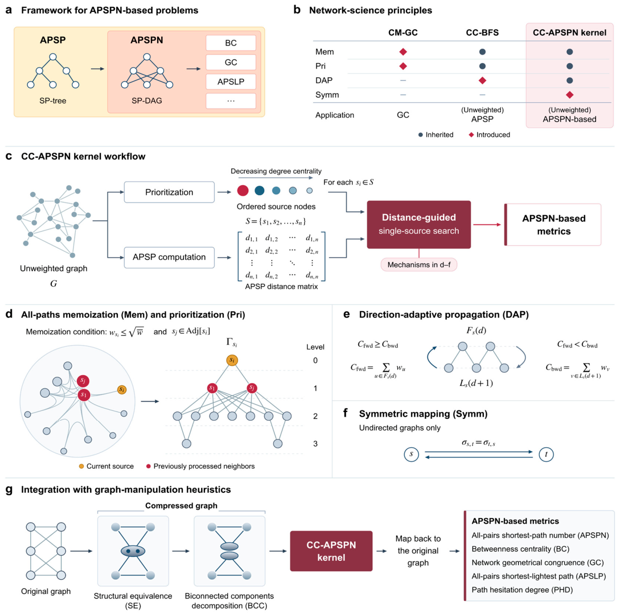
Figure 2.
| Sequential and parallel APSPN kernels on artificial hyperbolic scale-free networks. Runtimes are compared for the sequential Brandes-APSPN kernel (black squares), sequential CC-APSPN kernel (coral circles), and Parallel CC-APSPN kernel with 32 threads (crimson triangles). a, d, All-pairs shortest path number (APSPN) computation on low-density (a) and high-density (d) networks. b, e, Betweenness centrality (BC). c, f, Network geometrical congruence (GC). The number of nodes is , or . Low density is below 100,000 nodes and at 100,000 nodes; high density is and , respectively. Coral annotations show the percentage runtime reduction of sequential CC-APSPN relative to sequential Brandes-APSPN at 100,000 nodes; labels beside the three series give their runtimes. Networks were generated by the nonuniform popularity-similarity optimization (nPSO) model with temperature 0.1, power-law exponent and four communities. Points below 100,000 nodes show the mean over five independent network realizations. Each 100,000-node configuration has one realization, used by all algorithms. Error bars are omitted for they are negligible.
Figure 2.
| Sequential and parallel APSPN kernels on artificial hyperbolic scale-free networks. Runtimes are compared for the sequential Brandes-APSPN kernel (black squares), sequential CC-APSPN kernel (coral circles), and Parallel CC-APSPN kernel with 32 threads (crimson triangles). a, d, All-pairs shortest path number (APSPN) computation on low-density (a) and high-density (d) networks. b, e, Betweenness centrality (BC). c, f, Network geometrical congruence (GC). The number of nodes is , or . Low density is below 100,000 nodes and at 100,000 nodes; high density is and , respectively. Coral annotations show the percentage runtime reduction of sequential CC-APSPN relative to sequential Brandes-APSPN at 100,000 nodes; labels beside the three series give their runtimes. Networks were generated by the nonuniform popularity-similarity optimization (nPSO) model with temperature 0.1, power-law exponent and four communities. Points below 100,000 nodes show the mean over five independent network realizations. Each 100,000-node configuration has one realization, used by all algorithms. Error bars are omitted for they are negligible.
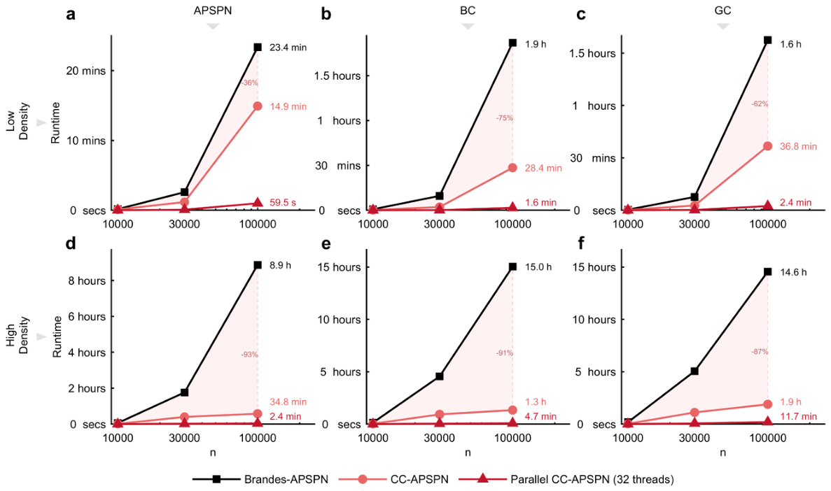
Figure 3.
| Sequential and parallel APSPN kernels across diverse network topologies (dense, ). Runtimes are compared on nonuniform popularity-similarity optimization (nPSO) networks with nodes and density . Rows vary the power-law exponent (a–c), temperature (d–f) or number of communities (g–i). Columns report all-pairs shortest path number (APSPN), betweenness centrality (BC) and network geometrical congruence (GC), respectively. Black squares, coral circles and crimson triangles denote the sequential Brandes-APSPN kernel, sequential CC-APSPN kernel and Parallel CC-APSPN kernel with 32 threads. Summary strips above each panel show the arithmetic mean runtime across the three displayed parameter settings. Runtime axes are logarithmic; bar lengths are proportional to the means on a linear scale within each panel. Unless varied, temperature is 0.1, , and the number of communities is four. Each parameter configuration uses one network realization shared by all algorithms.
Figure 3.
| Sequential and parallel APSPN kernels across diverse network topologies (dense, ). Runtimes are compared on nonuniform popularity-similarity optimization (nPSO) networks with nodes and density . Rows vary the power-law exponent (a–c), temperature (d–f) or number of communities (g–i). Columns report all-pairs shortest path number (APSPN), betweenness centrality (BC) and network geometrical congruence (GC), respectively. Black squares, coral circles and crimson triangles denote the sequential Brandes-APSPN kernel, sequential CC-APSPN kernel and Parallel CC-APSPN kernel with 32 threads. Summary strips above each panel show the arithmetic mean runtime across the three displayed parameter settings. Runtime axes are logarithmic; bar lengths are proportional to the means on a linear scale within each panel. Unless varied, temperature is 0.1, , and the number of communities is four. Each parameter configuration uses one network realization shared by all algorithms.
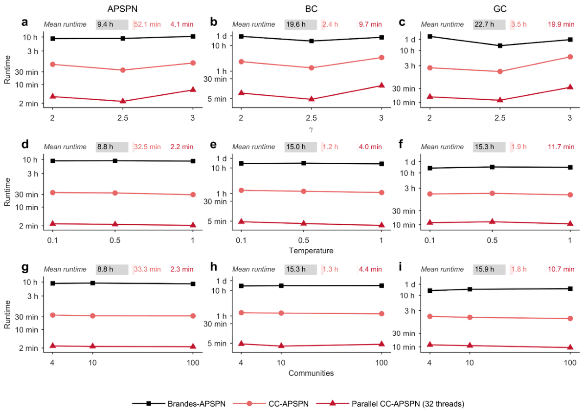
Figure 4.
| Sequential and parallel APSPN kernel performance for exact BC on real-world networks. Betweenness centrality (BC) runtimes are measured on 457 ATLAS networks with 5,000–200,000 nodes. a–c, Moving-average runtimes versus density , grouped by the number of nodes . d–f, Moving-average runtimes versus , grouped by . Black, coral and crimson curves show the sequential Brandes-APSPN kernel, sequential CC-APSPN kernel and Parallel CC-APSPN kernel with 32 threads, respectively; summary strips above a–f give arithmetic mean runtimes within each group, with bar lengths proportional to those means. g, h, Per-network comparisons of the two sequential kernels only, colored by density and size, respectively. The horizontal axis gives the sequential CC-APSPN kernel runtime and the vertical axis the sequential Brandes-APSPN kernel runtime; points above the diagonal favor the CC-APSPN kernel. Insets enlarge the lower-runtime region. Each algorithm is executed once per network. The parallel results appear only in a–f and their summary strips.
Figure 4.
| Sequential and parallel APSPN kernel performance for exact BC on real-world networks. Betweenness centrality (BC) runtimes are measured on 457 ATLAS networks with 5,000–200,000 nodes. a–c, Moving-average runtimes versus density , grouped by the number of nodes . d–f, Moving-average runtimes versus , grouped by . Black, coral and crimson curves show the sequential Brandes-APSPN kernel, sequential CC-APSPN kernel and Parallel CC-APSPN kernel with 32 threads, respectively; summary strips above a–f give arithmetic mean runtimes within each group, with bar lengths proportional to those means. g, h, Per-network comparisons of the two sequential kernels only, colored by density and size, respectively. The horizontal axis gives the sequential CC-APSPN kernel runtime and the vertical axis the sequential Brandes-APSPN kernel runtime; points above the diagonal favor the CC-APSPN kernel. Insets enlarge the lower-runtime region. Each algorithm is executed once per network. The parallel results appear only in a–f and their summary strips.
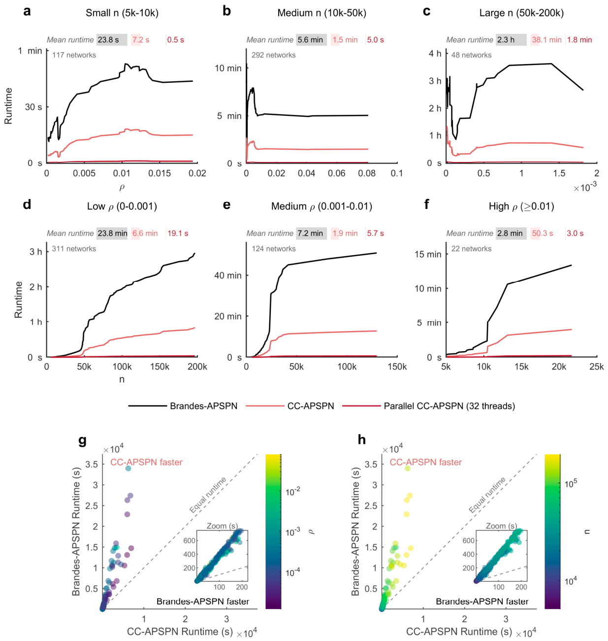
Figure 5.
| Graph manipulation amplifies the CC-APSPN kernel’s speedup. Betweenness centrality (BC) was benchmarked on ATLAS networks with 50,000–150,000 nodes; speedup is the sequential Brandes-APSPN kernel runtime divided by the tested method’s runtime. a, Grouped-dot comparison of the CC-APSPN kernel alone and combined with structural equivalence (SE), biconnected-components decomposition (BCC), or both. The ten networks with the greatest maximum speedup across variants are shown, in descending order of that maximum; labels give network name, node count and density . Small vertical offsets separate the four methods without encoding an additional quantity. b, Arithmetic mean speedup ± standard error across the same ten networks. The dashed 1× line marks parity with the Brandes-APSPN kernel. Combining SE and BCC gives the highest mean speedup.
Figure 5.
| Graph manipulation amplifies the CC-APSPN kernel’s speedup. Betweenness centrality (BC) was benchmarked on ATLAS networks with 50,000–150,000 nodes; speedup is the sequential Brandes-APSPN kernel runtime divided by the tested method’s runtime. a, Grouped-dot comparison of the CC-APSPN kernel alone and combined with structural equivalence (SE), biconnected-components decomposition (BCC), or both. The ten networks with the greatest maximum speedup across variants are shown, in descending order of that maximum; labels give network name, node count and density . Small vertical offsets separate the four methods without encoding an additional quantity. b, Arithmetic mean speedup ± standard error across the same ten networks. The dashed 1× line marks parity with the Brandes-APSPN kernel. Combining SE and BCC gives the highest mean speedup.
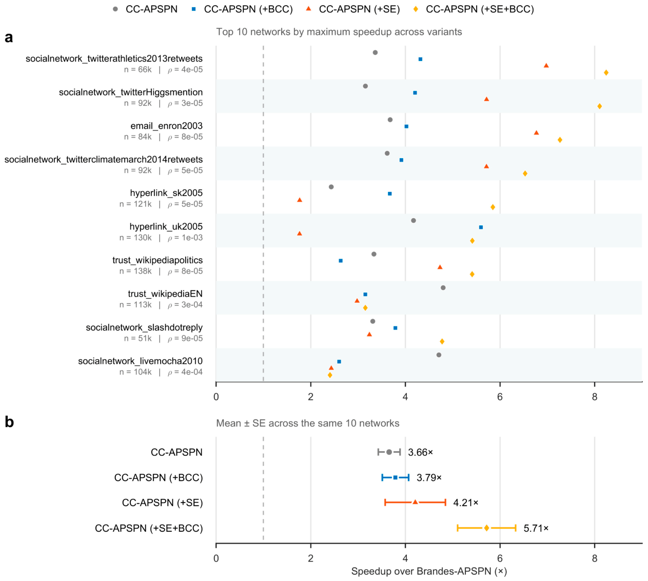
Figure 6.
| Approximating BC and GC with CC-bbBFS. a–c, Cannistraci–Chen balanced bidirectional breadth-first search (CC-bbBFS), the shared primitive for betweenness centrality (BC) and network geometrical congruence (GC) approximation. a, Sample a node pair and compute its shortest-path number . b, Expand the frontier with lower summed degree and combine path counts across meeting edges. For a source , , and denote its frontier, shortest-path number vector and distance vector. is node ’s degree. Subscripts and distinguish the endpoints and denotes the shortest-path number from to . c, Replay search states stored to depth before resuming balanced BFS. d–f, CC-ApproxBC, SILVAN and KADABRA on 343 ATLAS networks (10,000–300,000 nodes), 15 SILVAN networks and 21 nonuniform popularity-similarity optimization (nPSO) configurations, at absolute-error parameter and failure-probability parameter . Upper plots show mean runtime; lower plots show the means of maximum absolute error (MAE; blue, left axis) and mean relative absolute error over nodes with nonzero exact BC (MRAE; orange, right axis). BC is normalized by for undirected or for directed networks, where is node count. g, h, CC-ApproxGC on 430 ATLAS networks (1,000–100,000 nodes) and 21 nPSO configurations, showing mean runtime above mean absolute (blue) and relative (orange, %) errors. i, Error–runtime cost: the product of mean runtime and mean absolute error, each normalized by its minimum across sampling factors . Dashed lines mark the recommended range 1–5. For BC on ATLAS and SILVAN networks (d, e), each method is run five times per network, and the results are averaged within each network. For GC on ATLAS networks (g), each network is evaluated once at each sampling factor. For nPSO networks (f, h), each parameter configuration uses five independent realizations with one run on each. Results are averaged over the realizations. Accuracy error bars indicate standard errors of the mean across networks (d, e, g) or configuration means (f, h).
Figure 6.
| Approximating BC and GC with CC-bbBFS. a–c, Cannistraci–Chen balanced bidirectional breadth-first search (CC-bbBFS), the shared primitive for betweenness centrality (BC) and network geometrical congruence (GC) approximation. a, Sample a node pair and compute its shortest-path number . b, Expand the frontier with lower summed degree and combine path counts across meeting edges. For a source , , and denote its frontier, shortest-path number vector and distance vector. is node ’s degree. Subscripts and distinguish the endpoints and denotes the shortest-path number from to . c, Replay search states stored to depth before resuming balanced BFS. d–f, CC-ApproxBC, SILVAN and KADABRA on 343 ATLAS networks (10,000–300,000 nodes), 15 SILVAN networks and 21 nonuniform popularity-similarity optimization (nPSO) configurations, at absolute-error parameter and failure-probability parameter . Upper plots show mean runtime; lower plots show the means of maximum absolute error (MAE; blue, left axis) and mean relative absolute error over nodes with nonzero exact BC (MRAE; orange, right axis). BC is normalized by for undirected or for directed networks, where is node count. g, h, CC-ApproxGC on 430 ATLAS networks (1,000–100,000 nodes) and 21 nPSO configurations, showing mean runtime above mean absolute (blue) and relative (orange, %) errors. i, Error–runtime cost: the product of mean runtime and mean absolute error, each normalized by its minimum across sampling factors . Dashed lines mark the recommended range 1–5. For BC on ATLAS and SILVAN networks (d, e), each method is run five times per network, and the results are averaged within each network. For GC on ATLAS networks (g), each network is evaluated once at each sampling factor. For nPSO networks (f, h), each parameter configuration uses five independent realizations with one run on each. Results are averaged over the realizations. Accuracy error bars indicate standard errors of the mean across networks (d, e, g) or configuration means (f, h).
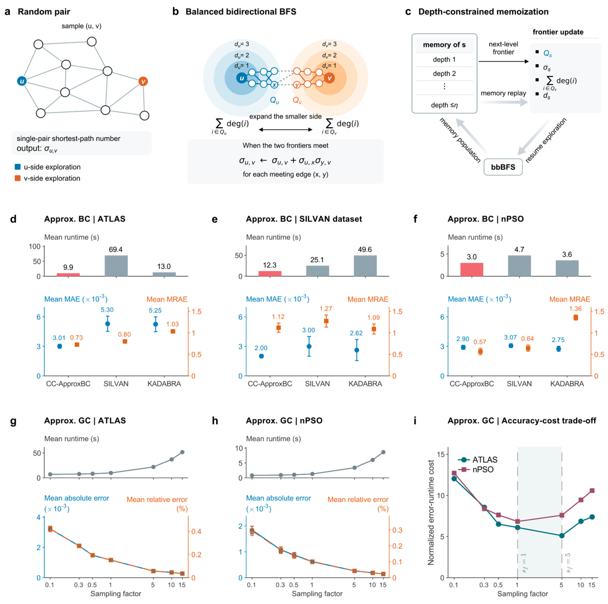
Supplementary Materials
The following supporting information can be downloaded at the website of this paper posted on Preprints.org. Correspondence and requests for materials should be addressed to Carlo Vittorio Cannistraci.
Author Contributions
C.V.C. conceived the study of the network-science-informed APSPN algorithm. J.C. and C.V.C. designed the all-paths memoization mechanism in the CC-APSPN kernel, the joint utilization of centrality-driven prioritization and direction-adaptive propagation, and the constraint strategy in memoization. J.C. and C.V.C. designed the symmetric mapping strategy and the CC-bbBFS single-pair primitive, as well as the depth-constrained memoization mechanism. J.C. implemented all algorithms and conducted the complexity analysis and correctness proofs under the supervision of C.V.C. J.C. and C.V.C. designed the experiments, and J.C. collected the data and conducted the experiments. C.V.C. and J.C. jointly analyzed the data and interpreted the results. J.C. and C.V.C. jointly wrote the manuscript. C.V.C. provided research infrastructure and financial support. All authors reviewed the manuscript. C.V.C. comprehensively supervised the project.
Funding
This work was supported by: The National Natural Science Foundation of China grant number W2531064 to C.V.C. The Zhou Yahui Chair Professorship award of Tsinghua University to C.V.C. The National High-Level Talent Program of the Ministry of Science and Technology of China grant number 20241710001 to C.V.C.
Data availability
Source data are provided with this article. The real-world networks used in this study are available from the ATLAS dataset https://www.dropbox.com/scl/fi/owtzfdtegcuesaux1dmyj/ATLAS_extended.zip?rlkey=07pukz jasvc2hkafgl5kukw7u&st=srr82jrr&dl=0 and the SILVAN article22. The artificial networks were generated using the nPSO and WS models with parameters specified in the article. Scripts for generating the networks and benchmarking the algorithms are available at https://github.com/biomedical-cybernetics/CC-APSPN.
Code availability
The source code of the Brandes-APSPN kernel, the CC-APSPN kernel (including its parallel implementation), the CC-bbBFS primitive with CC-ApproxBC and CC-ApproxGC, and the integration of the CC-APSPN kernel with graph manipulation heuristics (SE and BCC) is available at https://github.com/biomedical-cybernetics/CC-APSPN.
Acknowledgments
The authors thank Mo Yang for her administrative support.
Competing interests
The authors declare no competing interests.
References
- Watts, D. J.; Strogatz, S. H. Collective dynamics of ‘small-world’ networks. Nature 1998, 393, 440–442. [Google Scholar] [CrossRef] [PubMed]
- Newman, M. E. J. Models of the Small World. J. Stat. Phys. 2000, 101, 819–841. [Google Scholar] [CrossRef]
- Milgram, S. The small world problem. Psychol. Today 1967, 1, 60–67. [Google Scholar] [CrossRef]
- Sporns, O.; Zwi, J. D. The small world of the cerebral cortex. Neuroinformatics 2004, 2, 145–162. [Google Scholar] [CrossRef] [PubMed]
- Freeman, L. C. A Set of Measures of Centrality Based on Betweenness. Sociometry 1977, 40, 35–41. [Google Scholar] [CrossRef]
- Boguñá, M.; et al. Network geometry. Nat. Rev. Phys. 2021, 3, 114–135. [Google Scholar] [CrossRef]
- Allard, A.; Serrano, M. Á.; García-Pérez, G.; Boguñá, M. The geometric nature of weights in real complex networks. Nat. Commun. 2017, 8, 14103. [Google Scholar] [CrossRef] [PubMed]
- Brandes, U. A faster algorithm for betweenness centrality. J. Math. Sociol. 2001, 25, 163–177. [Google Scholar] [CrossRef]
- Brandes, U. On variants of shortest-path betweenness centrality and their generic computation. Soc. Netw. 2008, 30, 136–145. [Google Scholar] [CrossRef]
- Kitsak, M.; et al. Betweenness centrality of fractal and nonfractal scale-free model networks and tests on real networks. Phys. Rev. E 2007, 75, 056115. [Google Scholar] [CrossRef] [PubMed]
- Koschützki, D.; Schreiber, F. Centrality Analysis Methods for Biological Networks and Their Application to Gene Regulatory Networks. Gene Regul. Syst. Biol. 2008, 2, GRSB.S702. [Google Scholar] [CrossRef] [PubMed]
- Mahadevan, P.; et al. The internet AS-level topology: three data sources and one definitive metric. SIGCOMM Comput Commun. Rev. 2006, 36, 17–26. [Google Scholar]
- Cannistraci, C. V.; Muscoloni, A. Geometrical congruence, greedy navigability and myopic transfer in complex networks and brain connectomes. Nat. Commun. 2022, 13, 7308. [Google Scholar] [CrossRef] [PubMed]
- Kitsak, M.; et al. Finding shortest and nearly shortest path nodes in large substantially incomplete networks by hyperbolic mapping. Nat. Commun. 2023, 14, 186. [Google Scholar] [CrossRef] [PubMed]
- Zwick, U. All pairs lightest shortest paths. In Proceedings of the thirty-first annual ACM symposium on Theory of Computing 61–69; ACM: Atlanta Georgia USA, 1999. [Google Scholar] [CrossRef]
- Deng, Y.; Wu, J. Power law of path multiplicity in complex networks. PNAS Nexus 2024, 3, pgae228. [Google Scholar] [CrossRef] [PubMed]
- Deng, Y.; et al. Community structure unveils the path multiplicity in complex networks. Nat. Commun. 2026, 17, 2283. [Google Scholar] [CrossRef] [PubMed]
- Barabási, A.-L.; Dezső, Z.; Ravasz, E.; Yook, S.-H.; Oltvai, Z. Scale-free and hierarchical structures in complex networks. In AIP conference proceedings; American Institute of Physics, 2003; vol. 661, pp. 1–16. [Google Scholar] [CrossRef]
- Papadopoulos, F.; Kitsak, M.; Serrano, M. Á.; Boguñá, M.; Krioukov, D. Popularity versus similarity in growing networks. Nature 2012, 489, 537–540. [Google Scholar] [CrossRef] [PubMed]
- Ravasz, E.; Barabási, A.-L. Hierarchical organization in complex networks. Phys. Rev. E 2003, 67, 026112. [Google Scholar] [CrossRef] [PubMed]
- Chen, J.; Cannistraci, C. V. Accelerating All-Pairs Shortest Path Computation via Dynamic Programming Informed by Network Science. 2026. Available online: https://www.preprints.org/.
- Pellegrina, L.; Vandin, F. SILVAN: Estimating Betweenness Centralities with Progressive Sampling and Non-uniform Rademacher Bounds. ACM Trans. Knowl. Discov. Data 2024, 18, 1–55. [Google Scholar] [CrossRef]
- Borassi, M.; Natale, E. KADABRA is an ADaptive Algorithm for Betweenness via Random Approximation. ACM J. Exp. Algorithmics 2019, 24, 1–35. [Google Scholar] [CrossRef]
- Abboud, A.; Grandoni, F.; Vassilevska Williams, V. Subcubic Equivalences between Graph Centrality Problems, APSP, and Diameter. ACM Trans. Algorithms 2023, 19, 1–30. [Google Scholar] [CrossRef]
- Koschützki, D.; et al. Centrality Indices. In Network Analysis; Brandes, U., Erlebach, T., Eds.; Springer Berlin Heidelberg: Berlin, Heidelberg, 2005; vol. 3418, pp. 16–61. [Google Scholar]
- Chan, T. M.; Williams, V. V.; Xu, Y. Algorithms, Reductions and Equivalences for Small Weight Variants of All-Pairs Shortest Paths. 2021. [Google Scholar] [CrossRef]
- Nasre, M.; Pontecorvi, M.; Ramachandran, V. Decremental All-Pairs ALL Shortest Paths and Betweenness Centrality. In Algorithms and Computation; Ahn, H.-K., Shin, C.-S., Eds.; Springer International Publishing: Cham, 2014; vol. 8889, pp. 766–778. [Google Scholar]
- Simas, T.; Correia, R. B.; Rocha, L. M. The distance backbone of complex networks. J. Complex Netw. 2021, 9, cnab021. [Google Scholar] [CrossRef] [PubMed]
- Rozum, J. C.; Rocha, L. M. The ultrametric backbone is the union of all minimum spanning forests. J. Phys. Complex. 2024, 5, 035009. [Google Scholar] [CrossRef] [PubMed]
- Riondato, M.; Kornaropoulos, E. M. Fast approximation of betweenness centrality through sampling. In Proceedings of the 7th ACM international conference on Web search and data mining 413–422; ACM: New York New York USA, 2014. [Google Scholar] [CrossRef]
- Chehreghani, M. H.; Bifet, A.; Abdessalem, T. Efficient Exact and Approximate Algorithms for Computing Betweenness Centrality in Directed Graphs. In Advances in Knowledge Discovery and Data Mining; Phung, D., et al., Eds.; Springer International Publishing: Cham, 2018; vol. 10939, pp. 752–764. [Google Scholar]
- Suppa, P.; Zimeo, E. A Clustered Approach for Fast Computation of Betweenness Centrality in Social Networks. In 2015 IEEE International Congress on Big Data 47–54; IEEE: New York City, NY, USA, 2015. [Google Scholar] [CrossRef]
- McLaughlin, A.; Bader, D. A. Scalable and High Performance Betweenness Centrality on the GPU. In SC14: International Conference for High Performance Computing, Networking, Storage and Analysis 572–583; IEEE: New Orleans, LA, USA, 2014. [Google Scholar] [CrossRef]
- Puzis, R.; Zilberman, P.; Elovici, Y.; Dolev, S.; Brandes, U. Heuristics for Speeding Up Betweenness Centrality Computation. In 2012 International Conference on Privacy, Security, Risk and Trust and 2012 International Confernece on Social Computing 302–311; IEEE: Amsterdam, Netherlands, 2012. [Google Scholar] [CrossRef]
- Puzis, R.; Elovici, Y.; Zilberman, P.; Dolev, S.; Brandes, U. Topology manipulations for speeding betweenness centrality computation. J. Complex Netw. 2015, 3, 84–112. [Google Scholar] [CrossRef]
- Baglioni, M.; Geraci, F.; Pellegrini, M.; Lastres, E. Fast Exact Computation of betweenness Centrality in Social Networks. In 2012 IEEE/ACM International Conference on Advances in Social Networks Analysis and Mining; IEEE: Istanbul, 2012; pp. 450–456. [Google Scholar] [CrossRef]
- Sariyüce, A. E.; Kaya, K.; Saule, E.; Çatalyürek, Ü. V. Graph Manipulations for Fast Centrality Computation. ACM Trans. Knowl. Discov. Data 2017, 11, 1–25. [Google Scholar] [CrossRef]
- Daniel, C.; Furno, A.; Goglia, L.; Zimeo, E. Fast cluster-based computation of exact betweenness centrality in large graphs. J. Big Data 2021, 8, 92. [Google Scholar] [CrossRef]
- Li, Y.; et al. Hierarchical Decomposition for Betweenness Centrality Measure of Complex Networks. Sci. Rep. 2017, 7, 46491. [Google Scholar] [CrossRef] [PubMed]
- Erdős, D.; Ishakian, V.; Bestavros, A.; Terzi, E. A Divide-and-Conquer Algorithm for Betweenness Centrality. In Proceedings of the 2015 SIAM International Conference on Data Mining 433–441; Society for Industrial and Applied Mathematics: Philadelphia, PA, 2015. [Google Scholar] [CrossRef]
- Bentert, M.; Dittmann, A.; Kellerhals, L.; Nichterlein, A.; Niedermeier, R. An Adaptive Version of Brandes’ Algorithm for Betweenness Centrality. 2020. [Google Scholar] [CrossRef]
- Muscoloni, A.; Cannistraci, C. V. A nonuniform popularity-similarity optimization (nPSO) model to efficiently generate realistic complex networks with communities. New J. Phys. 2018, 20, 052002. [Google Scholar] [CrossRef]
- Klemm, K.; Eguíluz, V. M. Highly clustered scale-free networks. Phys. Rev. E 2002, 65, 036123. [Google Scholar] [CrossRef] [PubMed]
- Staudt, C. L.; Sazonovs, A.; Meyerhenke, H. NetworKit: A tool suite for large-scale complex network analysis. Netw. Sci. 2016, 4, 508–530. [Google Scholar] [CrossRef]
- Avena-Koenigsberger, A.; Misic, B.; Sporns, O. Communication dynamics in complex brain networks. Nat. Rev. Neurosci. 2018, 19, 17–33. [Google Scholar] [CrossRef] [PubMed]
- Wandelt, S.; Sun, X.; Feng, D.; Zanin, M.; Havlin, S. A comparative analysis of approaches to network-dismantling. Sci. Rep. 2018, 8, 13513. [Google Scholar] [CrossRef] [PubMed]
- Adler, T.; Grassia, M.; Liao, Z.; Mangioni, G.; Cannistraci, C. V. Latent geometry-driven network automata for complex network dismantling. In The fourteenth international conference on learning representations; 2026.
- Zeng, Q.; Liu, Y.; Tang, M.; Gong, J. Identifying super-spreaders in information–epidemic coevolving dynamics on multiplex networks. Knowl.-Based Syst. 2021, 229, 107365. [Google Scholar] [CrossRef]
- Ahlswede, R.; Cai, Ning; Li, S.-Y. R.; Yeung, R. W. Network information flow. IEEE Trans. Inf. Theory 2000, 46, 1204–1216. [Google Scholar] [CrossRef]
- Newman, M. E. J. A measure of betweenness centrality based on random walks. Soc. Netw. 2005, 27, 39–54. [Google Scholar] [CrossRef]
- Muscoloni, A.; Thomas, J. M.; Ciucci, S.; Bianconi, G.; Cannistraci, C. V. Machine learning meets complex networks via coalescent embedding in the hyperbolic space. Nat. Commun. 2017, 8, 1615. [Google Scholar] [CrossRef] [PubMed]
Disclaimer/Publisher’s Note: The statements, opinions and data contained in all publications are solely those of the individual author(s) and contributor(s) and not of MDPI and/or the editor(s). MDPI and/or the editor(s) disclaim responsibility for any injury to people or property resulting from any ideas, methods, instructions or products referred to in the content. |
© 2026 by the authors. Licensee MDPI, Basel, Switzerland. This article is an open access article distributed under the terms and conditions of the Creative Commons Attribution (CC BY) license (http://creativecommons.org/licenses/by/4.0/).
Copyright: This open access article is published under a Creative Commons CC BY 4.0 license, which permit the free download, distribution, and reuse, provided that the author and preprint are cited in any reuse.