

Submitted:
02 November 2026
Posted:
04 November 2026
You are already at the latest version
Abstract
In loss-minimizing model predictive control of induction motor drives, the torque reference is often enforced by a quadratic penalty. Since every newton-meter costs loss, it leaves a steady torque error, and its weight has no physical basis. The error is shown to equal \( λ_M/(2q_M M^* ) \), where \( λ_M \) is the marginal loss per unit torque of the loss-optimal steady state, and a penalty on the absolute torque error removes it once its weight, in W/(N·m), exceeds the largest \( λ_M \)below the reference. The closed form of \( λ_M \) is derived from a temperature-dependent machine and inverter loss model. For a 7.5 kW drive at 36 simulated operating points, the closed-loop threshold equaled the marginal loss at fixed flux, which coincides with \( λ_M \) except on the voltage-limit boundary (up to 15% lower). The nominal quadratic weight left errors of 0.46–3.88%; with exact measurements the absolute-value penalty kept them below 10-4%, also on pump and conveyor cycles, while the loss per unit of work changed by at most 0.6%. Without flux reservation it lowers and delays the torque during a current-limited flux rebuild, unlike a combined absolute-value and quadratic term. Field-orientation mismatch, measurement noise and dead time cause errors that the penalty does not remove.
Keywords:
economic model predictive control
; induction motor drive
; exact penalty function
; weighting factor
; loss minimization
; torque control
; Lagrange multiplier
; field orientation
; quadratic programming
1. Introduction
An induction motor (IM) driving a pump, fan or conveyor spends most of its operating hours well below rated torque. At rated flux, such a drive keeps paying for magnetizing current and core loss that the load does not need. Loss-minimizing control (LMC) lowers the rotor flux until the extra copper loss of the torque-producing current outweighs the saving in magnetizing and core loss [1,2]. Under the extended product approach of IEC 61800-9-2, the converter losses enter the same balance, because the power drive system is assessed as a whole [3].
Model predictive control (MPC) handles current and voltage limits explicitly and accepts objectives other than tracking errors, which has made it a common framework for AC drives [4,5,6,7]. Economic MPC (EMPC) minimizes the operating cost itself, here the electrical loss [8,9]. Loss-aware predictive torque and current controllers have been reported for traction and linear induction machines [10,11,12], and the efficiency-oriented MPC literature for AC motors has been surveyed recently [13]. In previous work, the authors proposed a thermally adaptive EMPC (TA-EMPC) for a 7.5 kW industrial drive [14]. It minimizes a temperature-coupled loss model of the machine and inverter, adapts the stator and rotor resistances with a sensorless thermal observer, and reserves flux ahead of predicted load rises.
With loss as the objective, the torque reference turns into a constraint, and how it is imposed decides what the drive actually delivers. A hard equality on the predicted torque can make the quadratic program (QP) infeasible while the flux is being rebuilt or the current limit is reached. A quadratic penalty avoids infeasibility but turns the constraint into a trade-off. Each newton-meter costs watts, so the optimizer settles slightly below the reference. In TA-EMPC the torque weight was set so that this error stayed below 0.5% at the rated point. The weight sweep in [14] showed the error falling tenfold for every tenfold increase of the weight (4.77%, 0.50%, 0.05% and 0.005% at 0.1, 1, 10 and 100 times the nominal weight). This scaling was reported but not explained, and no rule was given for other ratings or thermal states.
The choice of weighting factors has a long history in predictive drive control. Proposed remedies include empirical guidelines [15,16], imposed optimized weights [17], ranking and entropy methods [18,19] and sequential formulations without weights [20]. All of them were developed for finite-control-set MPC, where the competing terms are tracking errors of a similar kind. A systematic review of energy-efficient MPC for industrial IM drives lists weighting under an economic objective, where the terms have a physical and monetary meaning, among the open problems [21]. Optimization theory supplies two relevant tools: the exact-penalty property of the ℓ1 norm, used in MPC to soften constraints [22,23,24], and the interpretation of a Lagrange multiplier as the sensitivity of the optimal cost to its constraint [25]. To the authors’ knowledge, they have not yet been used to assign a physical value to the torque weight of a loss-minimizing drive controller.
In this paper the torque term of the EMPC is replaced by a penalty proportional to the absolute torque error. Its weight μM is expressed in W/(N·m) and is bounded from below by the marginal loss per unit torque λM of the loss-optimal steady state. The contributions are:
- a closed-form expression for the steady torque error of the quadratic penalty, εM = λM/(2qMM*), which accounts for the 1/qM scaling in [14] and predicts that a fixed weight loses accuracy at light load and at high winding temperature;
- a sufficient condition for zero steady error with the absolute-value penalty, the local condition μM > λM(M*), and the form both results take in a controller that holds the flux at its steady-state target, together with an analytic expression and a torque–speed map of λM for a 7.5 kW drive at 20 °C and 115 °C;
- a numerical check on the receding-horizon controller, by locating the smallest weight that gives zero steady error in closed loop at 36 operating points, including rated speed with an active voltage limit;
- a simulation study covering current-limited transients with and without the flux reservation of [14], two duty cycles, uncertainty of the loss model, field-orientation error caused by mismatched rotor parameters, current-measurement noise and inverter dead time.
2. Materials and Methods
2.1. Machine Model
The cage IM is modeled in the rotor-flux-oriented d–q frame with the amplitude-invariant transformation. Index 1 refers to the stator and index 2 to the rotor. The rotor flux linkage Ψ2 lies on the d-axis; the state vector is and the input is :
Here R1 and R2 are the stator and rotor resistances, L1, L2 and Lm the stator, rotor and magnetizing inductances, k2 = Lm/L2, , , zp the number of pole pairs, ω the mechanical speed and ω1 = zpω + k2R2i1q/Ψ2 the angular frequency of the stator field. The electromagnetic torque is
By (4), the same torque can be obtained with a high flux and a small i1q or with a low flux and a large i1q; LMC exploits this freedom.
2.2. Loss Model and Parameters
The controllable loss of the drive is taken from [14]:
where i2d = (Ψ2 − Lmi1d)/L2 and i2q = −k2i1q are the rotor current components and is the stator current amplitude. The coefficient aI = 3(UCE0 + UF0)/π + (6/π)fswEsw(Ud/Uref)/Iref collects the threshold-voltage conduction loss and the switching loss, and bI = 3(rCE + rF)/4 the slope-resistance conduction loss, following Equations (11) and (12) of [14]; with the data of Table 1, aI = 6.30 W/A and bI = 0.0338 Ω. The resistances vary as Rj(ϑj) = Rj,20[1 + αj(ϑj − 20)], j = 1,2.
Table 1 lists the parameters and their origin. Machine and inverter data are those of Tables 2 and 3 in [14]. The quantities marked “this study” are either not given there or were changed. The switching frequency was raised from 8 kHz in [14] to 10 kHz, so that one PWM period equals the sampling period of 100 µs and the controller updates the voltage reference once per carrier period. The temperature coefficient of the aluminum cage, α2 = 0.00408 K⁻¹, corresponds to the temperature constant of 225 K for aluminum in IEC 60034-2-1 [26]. The rated rotor flux linkage was set to Ψ2N = 0.90 Wb; with this value the stator voltage at the rated point, 311.7 V, just fits the linear modulation limit = 311.8 V. The rated torque, speed and current then follow from the model. The input blocking, the weights r and ρΨ and the flux envelope enter the controller of Section 2.4. The parameter set is representative of a 7.5 kW, 400 V, four-pole machine and is not a nameplate record of a specific motor.
2.3. Steady-State Economic Layer and the Marginal Loss per Unit Torque
For a torque reference M*, speed ω and winding temperatures ϑ = (ϑ1,ϑ2), the loss-optimal steady state is the solution of
where is the 16-sided polygon inscribed in the circle of radius Imax that the dynamic controller also uses (Section 2.4), so that every steady-state target is admissible for it; for the voltage the circle is used, which lies inside the voltage polygon of the controller. The steady-state relations are i1d = Ψ2/Lm, i1q = M*/(1.5zpk2Ψ2), u1d = R1i1d − ω1σL1i1q and u1q = R1i1q + ω1L1i1d, and . The minimizer Ψ2s serves as the flux target of the dynamic controller. The central quantity of this paper is the derivative of the optimal loss with respect to the torque reference,
By the sensitivity theorem of nonlinear programming [25], λM is the Lagrange multiplier of the equality M = M* in (8). It states how many watts of loss the last newton-meter of torque costs. While the current and voltage limits are inactive, the first-order conditions of (8) yield
The approximation neglects the dependence of the core loss on the slip frequency. Equation (10) shows how λM behaves. It rises with the winding resistances, and hence with temperature, and falls with the square of the flux. Under LMC the optimal flux grows roughly as at partial load, so λM stays nearly constant there. Once the flux reaches its upper bound, λM grows in proportion to the torque. If the current or voltage limit is active, the multiplier also carries the price of that limit, and (10) no longer applies. In general, λM is therefore computed by differences of P* with a step of ±0.05 N·m, central inside the feasible region and one-sided (backward) where M* + 0.05 N·m is infeasible. The steady-state layer stores Ψ2s and λM in look-up tables (LUTs) on a 53 × 31 grid over 0 ≤ M* ≤ 1.3MN and 0.05ωN ≤ ω ≤ ωN, one pair of tables per thermal state; beyond Mmax the value at the last feasible grid point is held.
2.4. Dynamic Economic MPC
Over the prediction horizon, ω and ω1 are frozen at their present values, which makes (1)–(3) linear. Exact zero-order-hold discretization with Ts = 100 µs gives xi+1 = Adxi + Bdui. The input is held over blocks of 1, 1 and 8 steps, so Nc = 3 input vectors cover the horizon N = 10, and condensing gives X = f0 + GU. At each step the controller solves
subject to the predicted dynamics; a 16-sided polygon circumscribing the circle , which admits at most 1/cos(π/16) − 1 ≈ 1.9% overmodulation; a 16-sided polygon inscribed in the circle ||i1,i||≤Imax at the end of each block; and Ψmin ≤ Ψ2,i ≤ Ψ2N at every step. The predicted torque error is ei = M* − Mi, where Mi is linearized about the shifted solution of the previous step, and ϕ(⋅) is the torque term of Section 2.5. The loss terms (6)–(7) are quadratic in x, except aII1m, which is replaced by its first-order expansion at the measured current. Since the loss is multiplied by Ts, the cost is an energy and ϕ must be given in watts. In (11), uj−1 for j = 0 is the input applied in the previous sampling period.
The horizon covers NTs = 1 ms, whereas the rotor time constant L2/R2 is 182 ms at 20 °C and 131 ms at 115 °C. Even with the full current Imax applied to the d-axis, the flux can change within one horizon by no more than 14 mWb, about 5% of the lower flux bound, so the flux trajectory is governed by the terminal term in (11), which pulls Ψ2,N toward the loss-optimal target. Its weight ρΨ was chosen so that the steady flux stays close to Ψ2s; at the simulated operating points the deviation was at most 0.23%. As an option, the target can be raised in advance of a load increase by the flux reservation of [14]: Ψ2s is evaluated at , where is the largest reference over a preview window of 100 ms. This is a simplified form of Equation (17) in [14] with the conservativeness factor set to 1. The QP is solved by the dual active-set method of Goldfarb and Idnani [27]. Figure 1 shows the controller structure.
2.5. Torque Term
Four forms of ϕ are compared. In the hard formulation (H), ei = 0 is imposed at the end of each input block, which gives Nc equality constraints. If this QP is infeasible, the step is solved with the quadratic formulation instead, the usual safeguard in practice. The quadratic formulation (Q) uses ϕQ(e) = qMe2 with qM in W/(N·m)², as in [14]. The absolute-value formulation (L1) uses ϕL1(e) = μM|e| with μM in W/(N·m). It is implemented with one slack variable sj per input block :
where nj is the number of steps in block j. Strictly, (12) is a block-wise majorant of the ℓ1 sum : inside a block it penalizes the largest error, as an ℓ∞ norm would. The two coincide when the error is constant within each block. In steady state the error of the first block, which determines the applied input, is zero; residual errors planned for the later blocks are discussed in Section 3.2. Relative to Q, the QP gains Nc variables and 2N + Nc inequality rows. The weight is either constant, a fixed multiple of , the largest λM over the operating envelope in the hot state (Section 2.6), or scheduled, , from the LUT of Section 2.3 (L1-S). The fourth formulation (L1+Q) adds both terms, ϕ(e) = μM|e| + qMe2. Since the derivative of qMe2 is zero at e = 0, the quadratic part does not shift the exactness threshold; it only raises the price of large transient errors.
The analysis uses the reduced steady-state problem, in which the flux is re-optimized for the delivered torque M and M is the only decision variable. Let Mmax(ω,ϑ) denote the largest torque for which (8) is feasible.
Proposition 1.
(bias of the quadratic penalty). Let P* be differentiable at the minimizer MQ of
for 0 ≤ M ≤ Mmax, and let 0 < MQ < Mmax. Then M* − MQ = λM(MQ)/(2qM), and the relative steady error is εM = λM(MQ)/(2qMM*).
Proof.
At an interior minimizer the derivative vanishes: λM(MQ) − 2qM(M* − MQ) = 0. □
Proposition 2.
(zero steady error with the absolute-value penalty). Let 0 < M* ≤ Mmax, let P* be absolutely continuous for 0 ≤ M ≤ Mmax with derivative λM almost everywhere, and let λM ≥ 0 almost everywhere for M* ≤ M ≤ Mmax. If μM > Λ(M*), where Λ(M*) is the essential supremum of λM for 0 ≤ M ≤ M*, then M = M* is the unique global minimizer of P*(M) + μM|M* − M| for 0 ≤ M ≤ Mmax.
Proof.
For M* < M ≤ Mmax,
, so the cost exceeds P*(M*) by at least μM(M − M*) > 0. For 0 ≤ M < M*,
, hence P*(M) + μM(M* − M) ≥ P*(M*) + (μM − Λ)(M* − M) > P*(M*). □
Proposition 2 is global on the admissible torque interval and needs neither convexity nor monotonicity of λM; the only assumptions are that P* does not decrease above the reference and that λM is essentially bounded for torques below it. Both hold on the envelope of this drive, where P* is continuous and piecewise differentiable, with kinks where a current or voltage limit becomes active. The condition is sufficient, not necessary. Since the cost P*(M) + μM(M* − M) has the left derivative λM(M*) − μM at M*, the weaker condition μM > λM(M*) already makes M* a strict local minimizer, and μM ≥ λM(M*) is necessary for any local minimum at M*. The two bounds differ where λM decreases with torque, which happens at partial load when the optimal flux leaves its lower bound. On a grid with steps of 0.005MN and 0.05ωN over the operating envelope defined in Section 2.6, Λ(M*)/λM(M*) reaches 1.277 (at M*≈ 0.49MN in the cold state); the scheduled weight therefore uses κ = 1.35, which satisfies the global condition everywhere.
Both propositions refer to the reduced problem, in which the flux follows the delivered torque. The dynamic controller differs in one respect: its terminal term holds the flux at the target Ψ2s(M*) of the reference. The marginal loss that it trades against the torque term is therefore at Ψ2 = Ψ2s(M*), and the arguments of both propositions apply with λM replaced by ; in particular, Proposition 1 becomes . By the envelope theorem, wherever no current or voltage limit is active in (8). Away from M* the two differ, because at fixed flux the copper loss makes nearly proportional to the torque, whereas λM includes the re-optimization of the flux. Where the voltage limit is active in (8), λM also contains the price of that limit, which does not enter , so that there.
The propositions describe the steady state of the reduced problem. Whether the receding-horizon QP, with its 1 ms horizon, linearization, input blocking and terminal term, has the same threshold is not implied by them. For a convex QP, the exact-penalty theorem [23,24] guarantees a finite threshold, equal to a norm of the multipliers of the torque constraints, but gives no value for it. Moreover, the controller optimizes over a short horizon around the present state and can only respond to the local condition. The threshold of the closed loop, denoted , was therefore determined directly. For each operating point, closed-loop simulations were repeated with different μM, and the smallest weight for which the steady error fell below 10−4% was located by bisection to a relative resolution of 1.4 × 10⁻⁵ (Section 3.2).
If M* > Mmax, the hard formulation has no solution. The absolute-value formulation remains feasible, but for a finite μM nothing in the propositions ensures that it delivers Mmax; its behavior in this case is examined numerically in Section 3.3. A simple remedy is to limit the reference to , which the steady-state layer computes together with Ψ2s and λM; Proposition 2 then applies to the limited reference. This option was not used in the simulations.
2.6. Simulation Setup and Metrics
The plant integrates the nonlinear model (1)–(4), with ω1 updated continuously, by the fourth-order Runge–Kutta method with five substeps per control period and zero-order-hold inputs; with twenty substeps, the torque in the sequence of Figure 4 changed by less than 10⁻⁸% of MN and the loss energy by less than 10⁻¹¹%. The inverter is represented by its average model; dead time is added only in scenario (vii). Except in scenarios (vi) and (vii), field orientation is ideal and the controller receives i1d, i1q and Ψ2 without error. The load imposes the speed (dynamometer mode), so the torque controller is tested without a speed loop; this is an idealization, and the interaction with a speed controller is not examined. Two thermal states are used: cold, ϑ1 = ϑ2 = 20 °C, and hot, ϑ1 = ϑ2 = 115 °C, the hot steady state of [14], at which R1 is 37.3% and R2 38.8% above the cold values. The thermal observer of [14] is represented by the true temperatures.
The quadratic baseline uses the weight qM,nom = λM/(2 ⋅ 0.005MN) = 52.1 W/(N·m)², evaluated at the cold rated point, i.e., the weight for which the first-order estimate λM(M*)/(2qMM*) of Proposition 1 gives 0.5% error at the rated point. This reproduces the selection rule stated in [14]; the absolute weight of [14] is not reported there. The operating envelope is 0 < M* ≤ min{1.25MN,Mmax(ω)}, 0.05ωN ≤ ω ≤ ωN. The constant absolute-value weight is = 68.0 W/(N·m), where = 56.7 W/(N·m) is the maximum of λM over this envelope in the hot state, evaluated on the grid of Section 2.5 and on the boundary M* = Mmax(ω). It is reached at rated speed on the voltage-limit boundary, at M* = 1.227MN; at rated speed and 115 °C the voltage limit bounds the torque to Mmax = 1.228MN. The dimensionless factor 1.2 is a margin for revisions of the loss model (Section 3.5). The scheduled weight uses κ = 1.35. Table 2 summarizes the weights used throughout the paper.
Eight scenarios are simulated: (i) steady operation at 18 operating points per thermal state, i.e., 36 points in total, with M*/MN ∈ {0.1, 0.25, 0.5, 0.75, 1.0, 1.25} at ω/ωN ∈ {0.5, 0.9} and M*/MN ∈ {0.1, 0.25, 0.5, 0.75, 1.0, 1.2} at ω = ωN, where the voltage limit is active at the highest torque, and weight sweeps at two further points, 0.5MN at 0.75ωN and 0.2MN at 0.5ωN; (ii) a torque sequence at 0.75ωN in the hot state, from 0.2MN to 0.9MN, then to 1.4MN, which exceeds the current limit, and back to 0.5MN, with and without flux reservation and for horizons N = 10, 20 and 40; (iii) a pump cycle following with speed set-points between 0.45ωN and 0.9ωN (12 s); (iv) an intermittent conveyor cycle at 0.75ωN with ten torque levels between 0.15MN and 0.9MN (10 s), with and without flux reservation; (v) a Monte Carlo study of loss-model uncertainty; (vi) a study of field-orientation error, in which the controller and its current-model flux estimator use perturbed values of R2 and Lm while the plant keeps the nominal ones; (vii) steady operation with current-measurement noise and uncompensated inverter dead time; and (viii) a numerical check of closed-loop convergence, by linearizing the one-step closed-loop map at each equilibrium and by simulating from perturbed initial states.
The metrics are the steady relative torque error εM = (M* − M)/M*, averaged over each plateau after 0.3 s of settling; the relative integral absolute error ; the loss energy ; the delivered mechanical work ; and the ratio Eloss/W. The last metric avoids crediting a controller with a saving that comes only from delivering less work. The simulations were written in Python 3.13 with NumPy 2.5 and SciPy 1.18; the QP solver is the quadprog implementation of the Goldfarb–Idnani method. To check reproducibility, the complete computation was repeated from Supplementary Material S1 in a newly created Python environment (NumPy 2.5.4, SciPy 1.18.1, quadprog 0.1.14); all values derived from the results, 30,806 in total, agreed with the stored ones to a relative tolerance of 10−6, except the measured QP solution times. Generative AI was used in this study as stated in the Acknowledgments.
3. Results
3.1. Marginal Loss Per Unit Torque
Figure 2 maps λM over the torque–speed plane together with contours of the loss-optimal flux. For 0.1MN ≤ M* ≤ min{1.25MN,Mmax}, λM lies between 13.1 and 37.6 W/(N·m) at 20 °C and between 17.1 and 56.7 W/(N·m) at 115 °C. Up to about 0.5MN the optimal flux is below its rated value and λM changes little (13.1–17.4 W/(N·m) cold, 17.1–21.5 W/(N·m) hot), in line with (10). In this range λM is largest at 0.1MN and decreases slightly with torque; the decrease begins where the optimal flux leaves its lower bound Ψmin, at about 0.06MN, i.e., below the range considered here. Above about 0.5MN the flux sits at Ψ2N, and λM grows in proportion to the torque. Near rated speed the voltage limit takes over at high torque; at ωN it becomes active above 1.01MN in the cold state and above 0.79MN in the hot state. The optimal flux then drops below Ψ2N and λM climbs steeply, up to = 56.7 W/(N·m) in the hot state. At the operating points of Table 4 where no limit is active, heating from 20 °C to 115 °C raises λM by 24–35%. The increase follows Rσ in (10) and is diluted by the inverter term, which does not depend on temperature. At the 2 points at rated speed where the voltage limit is active in at least one of the two states, the increase reaches 58%, because the larger resistive voltage drop of the hot machine tightens the voltage limit and forces a lower flux.
Table 3 compares the closed form (10) with differences of P*. At these points no limit is active, the exact expression reproduces the numerical derivative to within 0.01%, and the simplified form differs by at most 0.4%.

Table 3.
Marginal loss per unit torque: numerical derivative of P* and Equation (10).
| ϑ, °C | M*/MN | ω/ωN | Ψ2s, Wb | λM, numerical, W/(N·m) | λM, Eq. (10), exact, W/(N·m) | λM, Eq. (10), approx., W/(N·m) |
|---|---|---|---|---|---|---|
| 20 | 0.1 | 0.5 | 0.394 | 15.98 | 15.98 | 15.95 |
| 20 | 0.25 | 0.5 | 0.627 | 14.40 | 14.40 | 14.37 |
| 20 | 0.5 | 0.5 | 0.891 | 13.61 | 13.61 | 13.57 |
| 20 | 0.5 | 0.9 | 0.858 | 14.69 | 14.69 | 14.64 |
| 20 | 1 | 0.5 | 0.900 | 25.61 | 25.61 | 25.58 |
| 20 | 1 | 0.9 | 0.900 | 25.63 | 25.63 | 25.58 |
| 20 | 1.25 | 0.5 | 0.900 | 31.59 | 31.59 | 31.55 |
| 115 | 0.1 | 0.5 | 0.398 | 20.05 | 20.05 | 20.01 |
| 115 | 0.25 | 0.5 | 0.634 | 18.47 | 18.47 | 18.43 |
| 115 | 0.5 | 0.5 | 0.900 | 17.70 | 17.70 | 17.66 |
| 115 | 0.5 | 0.9 | 0.874 | 18.80 | 18.80 | 18.72 |
| 115 | 1 | 0.5 | 0.900 | 34.33 | 34.33 | 34.28 |
| 115 | 1 | 0.9 | 0.900 | 34.36 | 34.36 | 34.28 |
| 115 | 1.25 | 0.5 | 0.900 | 42.48 | 42.48 | 42.44 |
3.2. Steady-State Torque Accuracy
Figure 3a shows the steady error of the quadratic formulation for weights from 0.1 to 100 times qM,nom. Over three decades the simulated errors follow the 1/qM law of Proposition 1. Across the 36 operating points of Table 4, the simulated error is 0.82–0.98 times the estimate of Proposition 1 for the reduced problem and 0.888–0.978 times its fixed-flux form (Section 2.5). Two effects account for the difference. First, the two estimates differ at light load, where , and on the voltage-limit boundary at rated speed. Second, input blocking lowers the error: with all inputs free (N = Nc = 10) the ratio to the fixed-flux estimate was 0.997–1.001, and the blocking used here reduced the error by 2.2–10.9%. With the nominal weight the error ranges from 0.46% to 3.88%, a spread by a factor of 8.4 for a weight that does not change; it is largest at 0.1MN in the hot state. Both trends, 1/M* at light load and the growth of Rσ with temperature, are those of Proposition 1 and Equation (10).
Figure 3b shows the absolute-value formulation. Below the threshold the controller sheds torque, and the error follows εM ≈ 1 − μM/λM: at fixed flux the marginal loss is nearly proportional to the torque, so the optimizer lowers the torque until its marginal loss equals μM. At μM = 0.95λM the error was 5.1–5.6%, at μM = λM at most 0.19%, and from μM = 1.05λM upward it fell below 10−4% in all four cases.
For the receding-horizon controller, the closed-loop threshold (Section 2.5) was 0.999–1.002 times the fixed-flux marginal loss at the 36 operating points (Table 4). Relative to λM(M*) it was 0.850–1.002; the 3 points with a ratio clearly below 1 all lie on the voltage-limit boundary at rated speed, where is 0.849–0.902 times λM(M*). The 1 ms horizon, the linearization, the input blocking and the terminal flux term thus leave the local threshold unchanged to within 0.2%, and up to this tolerance λM(M*) is an upper bound for it on this drive. At 18 of the points, λM decreases somewhere below M*, and the global bound Λ(M*) of Proposition 2 is up to 1.266 times λM(M*); the closed loop is nevertheless exact from the local threshold on, because the controller only sees the local trade-off. The constant weight of 68.0 W/(N·m) exceeds at all points by a factor of at least 1.47. A stricter requirement, zero predicted error at every step of the horizon, would call for weights of 0.88–3.92 times λM, and the constant weight is below this value at one point. It is not needed: the residual predicted errors appear in the later blocks, mostly in the held last block, where the planned drift of the flux toward its target cannot be compensated by a constant input, and they never reach the plant, because only the first input is applied and the predicted error of the first step was at most 10⁻¹⁵ of the reference.
Table 4.
Steady relative torque error and loss at 36 operating points: quadratic term with qM,nom (Q) and absolute-value formulations with μM = 68.0 W/(N·m) (L1, L1+Q) and κ = 1.35 (L1-S).
Table 4.
Steady relative torque error and loss at 36 operating points: quadratic term with qM,nom (Q) and absolute-value formulations with μM = 68.0 W/(N·m) (L1, L1+Q) and κ = 1.35 (L1-S).
| ϑ, °C | M*/MN | ω/ωN | λM, W/(N·m) | Λ/λM | Q: Prop. 1, % | Q: fixed flux, % | Q: sim., % | ΔP, W | ||
|---|---|---|---|---|---|---|---|---|---|---|
| 20 | 0.1 | 0.5 | 16.0 | 1.000 | 1.078 | 1.002 | 3.13 | 3.03 | 2.96 | 2.3 |
| 20 | 0.25 | 0.5 | 14.4 | 1.000 | 1.196 | 1.002 | 1.12 | 1.11 | 1.06 | 1.9 |
| 20 | 0.5 | 0.5 | 13.6 | 1.000 | 1.266 | 1.001 | 0.53 | 0.53 | 0.49 | 1.6 |
| 20 | 0.75 | 0.5 | 19.6 | 1.000 | 1.000 | 1.002 | 0.51 | 0.51 | 0.48 | 3.6 |
| 20 | 1 | 0.5 | 25.6 | 1.000 | 1.000 | 1.002 | 0.50 | 0.50 | 0.48 | 6.3 |
| 20 | 1.25 | 0.5 | 31.6 | 1.000 | 1.000 | 1.002 | 0.49 | 0.49 | 0.48 | 9.7 |
| 20 | 0.1 | 0.9 | 17.0 | 1.000 | 1.060 | 1.001 | 3.34 | 3.23 | 3.10 | 2.6 |
| 20 | 0.25 | 0.9 | 15.5 | 1.000 | 1.168 | 1.000 | 1.21 | 1.19 | 1.10 | 2.1 |
| 20 | 0.5 | 0.9 | 14.7 | 1.000 | 1.231 | 1.000 | 0.57 | 0.57 | 0.51 | 1.8 |
| 20 | 0.75 | 0.9 | 19.6 | 1.000 | 1.000 | 1.001 | 0.51 | 0.51 | 0.47 | 3.5 |
| 20 | 1 | 0.9 | 25.6 | 1.000 | 1.000 | 1.001 | 0.50 | 0.50 | 0.47 | 6.1 |
| 20 | 1.25 | 0.9 | 31.6 | 1.000 | 1.000 | 1.002 | 0.49 | 0.49 | 0.47 | 9.5 |
| 20 | 0.1 | 1 | 17.4 | 1.000 | 1.059 | 1.001 | 3.40 | 3.29 | 3.14 | 2.7 |
| 20 | 0.25 | 1 | 15.8 | 1.000 | 1.164 | 1.000 | 1.24 | 1.22 | 1.12 | 2.2 |
| 20 | 0.5 | 1 | 15.0 | 1.000 | 1.225 | 1.000 | 0.59 | 0.58 | 0.52 | 1.9 |
| 20 | 0.75 | 1 | 19.6 | 1.000 | 1.000 | 1.000 | 0.51 | 0.51 | 0.46 | 3.4 |
| 20 | 1 | 1 | 25.6 | 1.000 | 1.000 | 1.001 | 0.50 | 0.50 | 0.46 | 6.1 |
| 20 | 1.2 | 1 | 35.4 | 0.898 | 1.000 | 0.899 | 0.57 | 0.51 | 0.49 | 9.5 |
| 115 | 0.1 | 0.5 | 20.1 | 1.000 | 1.062 | 1.001 | 3.93 | 3.77 | 3.69 | 3.6 |
| 115 | 0.25 | 0.5 | 18.5 | 1.000 | 1.153 | 1.001 | 1.44 | 1.42 | 1.36 | 3.1 |
| 115 | 0.5 | 0.5 | 17.7 | 1.000 | 1.204 | 1.001 | 0.69 | 0.69 | 0.65 | 2.8 |
| 115 | 0.75 | 0.5 | 26.1 | 1.000 | 1.000 | 1.001 | 0.67 | 0.67 | 0.65 | 6.4 |
| 115 | 1 | 0.5 | 34.3 | 1.000 | 1.000 | 1.001 | 0.67 | 0.67 | 0.65 | 11.4 |
| 115 | 1.25 | 0.5 | 42.5 | 1.000 | 1.000 | 1.002 | 0.66 | 0.66 | 0.64 | 17.7 |
| 115 | 0.1 | 0.9 | 21.2 | 1.000 | 1.053 | 1.000 | 4.14 | 3.98 | 3.83 | 3.9 |
| 115 | 0.25 | 0.9 | 19.6 | 1.000 | 1.138 | 0.999 | 1.53 | 1.51 | 1.40 | 3.4 |
| 115 | 0.5 | 0.9 | 18.8 | 1.000 | 1.186 | 0.999 | 0.73 | 0.73 | 0.66 | 3.1 |
| 115 | 0.75 | 0.9 | 26.1 | 1.000 | 1.000 | 1.000 | 0.68 | 0.67 | 0.63 | 6.2 |
| 115 | 1 | 0.9 | 34.4 | 1.000 | 1.000 | 1.001 | 0.67 | 0.67 | 0.63 | 11.1 |
| 115 | 1.25 | 0.9 | 42.5 | 1.000 | 1.000 | 1.001 | 0.66 | 0.66 | 0.63 | 17.3 |
| 115 | 0.1 | 1 | 21.5 | 1.000 | 1.048 | 1.000 | 4.21 | 4.04 | 3.88 | 4.0 |
| 115 | 0.25 | 1 | 19.9 | 1.000 | 1.130 | 0.999 | 1.56 | 1.53 | 1.42 | 3.5 |
| 115 | 0.5 | 1 | 19.2 | 1.000 | 1.177 | 0.999 | 0.75 | 0.74 | 0.67 | 3.1 |
| 115 | 0.75 | 1 | 26.1 | 1.000 | 1.000 | 1.000 | 0.68 | 0.68 | 0.63 | 6.2 |
| 115 | 1 | 1 | 40.4 | 0.902 | 1.000 | 0.903 | 0.78 | 0.71 | 0.67 | 12.5 |
| 115 | 1.2 | 1 | 54.4 | 0.849 | 1.000 | 0.850 | 0.87 | 0.75 | 0.71 | 20.3 |
: marginal loss at the flux Ψ2s(M*). Λ/λM: ratio of the bound of Proposition 2 to the local value. : closed-loop threshold. Q, Prop. 1: estimate of Proposition 1 with λM at the delivered torque; Q, fixed flux: the same with . The errors of L1, L1-S and L1+Q were below 10−4% at every point and are not listed. ΔP: loss of L1 minus loss of Q.
The last column of Table 4 shows the price of the torque error. At every point Q dissipates less than L1, by 1.6–4.0 W up to 0.5MN and by at most 20.3 W (at 1.2MN, ωN, 115 °C), because it delivers less torque. The difference corresponds to the marginal loss of the missing torque, λM(M* − M); their ratio is 0.89–1.05. The lower loss of Q is thus the cost of under-delivery, not a better operating point, and the comparison at equal delivered work is made in Section 3.4.
3.3. Transients, Current Limit and Flux Reservation
Figure 4 shows the torque sequence in the hot state without flux reservation. Before the first step the machine runs at 0.2MN with the loss-optimal flux of 0.56 Wb. The step to 0.9MN is therefore limited by the current bound until the flux has been rebuilt. The step to 1.4MN asks for more than can be delivered within the current limit, Mmax = 1.300MN at this speed. Table 5 lists the metrics.
Figure 4.
Torque, rotor flux and stator current amplitude during a torque sequence at 0.75ωN, 115 °C, without flux reservation: (a) the step from 0.2MN to 0.9MN; (b) the whole sequence, with a reference of 1.4MN beyond the current limit between 350 and 550 ms. L1-S is listed in Table 5.
Figure 4.
Torque, rotor flux and stator current amplitude during a torque sequence at 0.75ωN, 115 °C, without flux reservation: (a) the step from 0.2MN to 0.9MN; (b) the whole sequence, with a reference of 1.4MN beyond the current limit between 350 and 550 ms. L1-S is listed in Table 5.
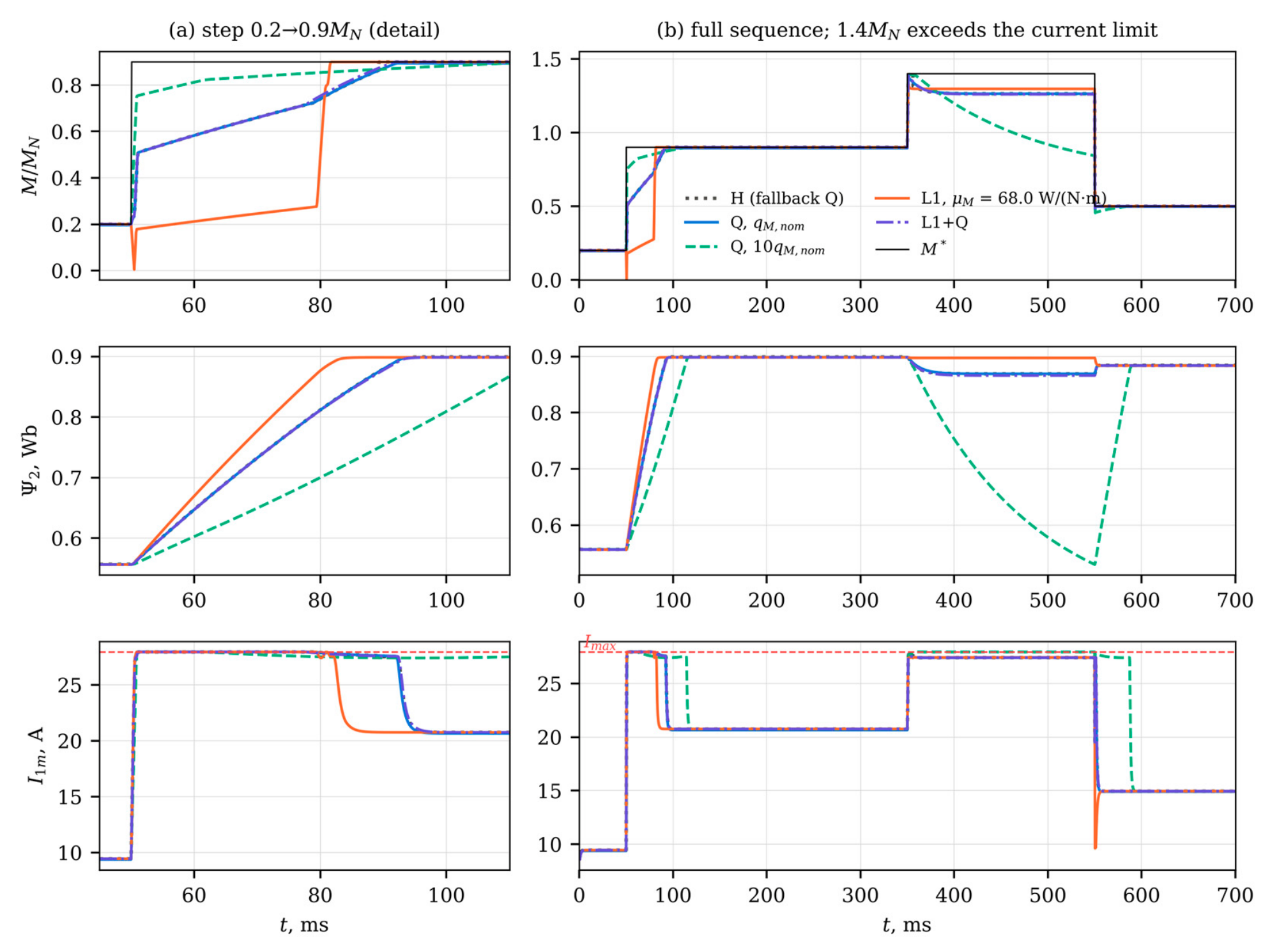
After the step all formulations first run at the current limit, and the torque rise is set by how fast the flux can be rebuilt. Q with qM,nom divides the current between i1d and i1q and reaches 90% of the step after 36.5 ms. With 10qM,nom more current goes to i1q; the 90% point is reached after 15.5 ms, at the price of a slower flux build-up. L1 behaves differently. Its penalty grows only linearly with the error, so the terminal flux term dominates during the rebuild: the current is spent on the flux first. The torque even falls below its initial value, practically to zero, stays below 0.2MN for 6.7 ms, and reaches half of the step only after 30.2 ms, against 6.0 ms for Q. Its IAErel over the step is 7.56%, against 4.07% for Q; L1-S behaves like L1 (7.71%), and L1+Q follows the quadratic transient (3.47%). In steady state Q settles at 0.894MN and 0.497MN, whereas all formulations with the absolute-value term deliver 0.900MN and 0.500MN. H also reaches the reference in steady state, but its QP was infeasible in 33.5% of the steps of the sequence, which were covered by the quadratic fallback.
Under the 1.4MN reference, L1 keeps the flux at 0.897 Wb or above and holds 1.297MN, practically the largest torque admissible under the current polygon, Mmax = 1.300MN. Q with qM,nom and L1+Q hold 1.267MN and 1.264MN with a flux of 0.869 Wb and 0.866 Wb at its lowest. With 10qM,nom, the controller keeps shifting current from i1d to i1q to shrink a large predicted error over a 1 ms horizon; the flux decays to 0.53 Wb, and the torque, 1.05MN on average over the interval (Table 5), falls to 0.85MN by its end. This flux depletion results from a large quadratic weight combined with a horizon much shorter than the rotor time constant. It is not a property that the absolute-value term guarantees to avoid, and the behavior of L1 at the current limit is an observation for this scenario.
Figure 5 and the lower part of Table 5 identify the cause of the L1 delay. With flux reservation, the 100 ms preview sees the step in advance and the flux is raised from 0.56 Wb to 0.90 Wb before it, which costs 91 W of additional steady-state loss while the load is still at 0.2MN. When the target is raised, all three formulations briefly lose torque, down to 0.05MN for Q and 0.00MN for L1; averaged over the 50 ms before the step, the torque is 0.197–0.199MN. The 90% rise time then drops to 1.1 ms for Q, 1.2 ms for L1 and 1.1 ms for L1+Q, and the IAErel of the step to 0.78%, 0.15% and 0.14%. With reservation, L1 and L1+Q have the smallest integral errors, because Q keeps its steady bias. Lengthening the horizon without reservation changes little: for L1 the time to half of the step is 30.2, 29.3 and 27.5 ms for N = 10, 20 and 40, since even 4 ms remains short compared with the rotor time constant of 131 ms. The delay of L1 in Figure 4 is therefore a consequence of rebuilding the flux under a short horizon, not of the absolute-value term as such.
3.4. Duty Cycles
Table 6 and Figure 6 summarize the duty cycles. In the hot state, Q with qM,nom leaves a mean plateau error of 0.97% on the pump cycle and 1.26% on the conveyor cycle, and 0.1qM,nom raises it to 9.2% and 11.4%. Without flux reservation, all formulations with the absolute-value term, including and the scheduled weight, bring the plateau error below 10−4% in both thermal states.
For the same reservation setting, the loss energy per unit of work hardly depends on the formulation. Without reservation, the absolute-value formulations change Eloss/W relative to Q with qM,nom by +0.03% to +0.57% of its value; across all hot-state runs without reservation, Eloss/W spans 17.89–18.02% on the pump cycle and 19.78–19.89% on the conveyor cycle. On the pump cycle the reference changes along speed ramps, and the integral error is almost entirely steady bias: IAErel is 0.79% for Q and below 0.001% with the absolute-value term. The conveyor cycle contains four steps from a lighter to a heavier load. Here L1 without reservation reaches an IAErel of 1.44–1.75%, close to the 1.63% of Q, because the zero plateau error is offset by the delayed rise after each step (Section 3.3). L1+Q lowers it to 0.75%; 10qM,nom reaches 0.36% but leaves a plateau error of 0.12%. With flux reservation, IAErel falls to 0.95% for Q, 0.17% for L1 and 0.08% for L1+Q, while Eloss/W rises to 19.94%, 19.96% and 19.95% because of the higher standby flux; reservation itself thus adds 0.10–0.16 percentage points on the conveyor cycle. The plateau errors of L1 and L1+Q with reservation, 0.17% and 0.05%, arise in the last 100 ms before a load increase, while the flux is being raised; over the rest of the plateaus the mean error of L1 is below 10−4%. In these windows the error of Q departs from its steady bias by up to 4.2 percentage points and that of L1 reaches 3.4%, so the deviation is caused by the flux ramp rather than by the form of the torque term. H needed its fallback in 0.0% and 1.5% of the steps of the two cycles; on the conveyor cycle its IAErel was 0.74%.
3.5. Uncertainty of the Loss Model
The torque equation (4) does not contain the loss coefficients kh, ke, aI and bI. Errors in these coefficients therefore change the flux chosen by the controller and the loss it incurs, but not the torque it delivers, and exactness is decided by λM of the controller’s own loss model, against which μM was set. The relevant question for a constant weight is therefore whether it can be fixed in advance when the loss model of the controller is revised later, for example after a new identification of the coefficients or by online adaptation. In 1500 Monte Carlo samples, kh, ke, aI and bI were scaled by four independent factors drawn uniformly from [0.7, 1.3], and the winding temperature was drawn uniformly from 20–115 °C. For each sample, λM was computed at 18 operating points: the 12 points at 0.5ωN and 0.9ωN of Table 4 and the six torque levels at rated speed, where the voltage limit becomes active at the highest torques; all 27,000 point evaluations were feasible for the perturbed models. Figure 7a shows the result. λM ranged from 13.0 to 55.2 W/(N·m); at the 12 points below rated speed it did not exceed 43.2 W/(N·m), and the larger values all occurred at rated speed. The constant weight μM = 68.0 W/(N·m) stayed above the per-sample maximum in all samples; it exceeds the largest sampled value by 23% and the 99th percentile of the per-sample maximum, 54.5 W/(N·m), by 25%. With the scheduled weight the condition holds by construction, since λM is taken from the same loss model that the optimizer uses. The temperature range matters as well: λM grows with the winding temperature, and the constant weight was set for the hot state of [14]. At 155 °C, the limit of thermal class F, the largest λM over the envelope of the nominal model is 65.8 W/(N·m), still below μM.
3.6. Field-Orientation Error
The results so far assume ideal field orientation. To show how the penalty-induced error compares with the error caused by wrong rotor parameters, the controller was given values of R2 and Lm perturbed by uniform factors in [1 − ε,1 + ε] and [1 − ε/2,1 + ε/2], following the perturbation scheme of [14], while the plant kept the nominal values. An error of R2 by ε also represents an error of the rotor temperature estimate, about 7 K for ε = 2% and 34 K for 10% at 115 °C. The controller estimates the flux with the current model and orients its frame with the estimated slip; the plant is simulated with both rotor flux components in that frame, so the torque on the shaft is . For each ε ∈ {2%,10%}, 100 samples were simulated at two operating points in the hot state (Table 7, Figure 7b). With correct parameters the errors of L1 are zero and those of Q equal the penalty bias, 1.36% and 0.63%. With mismatch, the true error of both formulations is dominated by the orientation error, which reaches several percent at ε = 10%. For the same perturbed parameters, the true error of Q exceeds that of L1 by a median of 1.37 and 0.65 percentage points at ε = 10% for the two operating points (5th–95th percentiles 1.01–1.69 and 0.32–0.97), which is close to the penalty bias of Q at these points. The two contributions thus add up, and the absolute-value term removes one of them. The error of the torque estimated by the controller is also nonzero with mismatch (median absolute value 0.19% for L1 over both values of ε and both points), because the prediction model no longer matches the plant and the controller has no integral action; this offset is of the kind addressed by offset-free MPC [28].
3.7. Measurement Noise and Dead Time
The results above assume exact measurements and an ideal inverter. Two disturbances were therefore added at three operating points in the hot state (Table 8). Gaussian noise with a standard deviation σi of 0.1 A or 0.4 A, about 0.45% and 1.8% of I1N, was added to both measured current components at every sample, and the controller estimated the flux with the current model driven by the noisy i1d. Dead time was represented by its average effect, a voltage vector of amplitude (4/π)tdfswUd = 13.8 V opposite to the current vector for td = 2 µs, which the controller did not compensate. Each run lasted 0.6 s, the statistics were taken over its last 0.3 s, and each case with noise was repeated with 10 noise realizations.
With measurement noise the absolute-value term is no longer exact. The mean error of L1 was 0.01–0.15% for σi = 0.1 A and 0.48–0.69% for 0.4 A, largest at light load, whereas the error of Q changed by at most 0.01 percentage points for 0.1 A and by −0.03 to +0.23 percentage points for 0.4 A; the 95% confidence intervals are at most ±0.13 percentage points wide. The error of L1 stayed below that of Q at every point, but a weight above λM does not ensure zero error once the measured torque fluctuates around the reference. A diagnostic run with the term aII1m linearized at the noise-free current instead of the measured one left the error of L1 at 0.1MN, 0.5ωN and σi = 0.4 A unchanged (0.69% in both cases), so the upward bias of the amplitude of a noisy current is not the cause. The origin of the bias was not identified. The kink of |e| is a plausible contributor for L1, since below the reference the loss term opposes the penalty and above it adds to it, so that apparent excesses of torque are corrected more strongly than apparent shortfalls; however, the error of Q also changes with noise, by −0.03 to +0.23 percentage points at 0.4 A, so part of the effect is common to both formulations. Uncompensated dead time produced a steady offset of 0.93–2.55% for L1 and L1+Q and raised the error of Q by 1.14–3.70 percentage points. Like the orientation error of Section 3.6, this offset comes from a mismatch between the prediction model and the plant, and the absolute-value term does not remove it.
No self-sustained chattering was observed: with dead time but without noise, all formulations settled to a constant input. With noise, L1 passed more of it to the input than Q. The RMS change of the voltage vector between samples was 1.6–2.2 times that of Q for σi = 0.1 A and 1.2–1.3 times for 0.4 A, and the standard deviation of the shaft torque was 8–12% higher at 0.4 A. L1+Q behaved similarly, with slightly smaller noise-induced errors at light load.
3.8. Closed-Loop Behavior
The propositions concern the equilibrium, not convergence to it, and no stability proof is available for the nonsmooth absolute-value term. Three numerical checks were therefore made (Table 9). First, the one-step closed-loop map, with the plant state and the previous input as its state, was linearized at the equilibrium of each of the 36 operating points by finite differences, in both directions along each coordinate. The state of the map contains the rotor flux, so the flux dynamics are part of the test. The open-loop rotor pole, = 0.9992 at 115 °C, does not appear in the closed-loop spectrum, because the controller acts on the flux through i1d. The winding temperatures, which change over minutes, are treated as parameters. The largest spectral radius was 0.9084 for Q, 0.9254 for L1 and 0.9254 for L1+Q; the slowest mode of these linearizations has a time constant of at most 1.29 ms. L1 and L1+Q give the same spectral radius to four decimals at 35 of the 36 points (largest difference 1.5 × 10⁻⁴): at the equilibrium the slack constraints hold the predicted error at zero, and the quadratic term, whose gradient vanishes there, hardly changes the local control law. Because the control law of a QP is piecewise affine and, with the absolute-value term, the equilibrium lies where several affine pieces meet, a linearization along the coordinate directions need not represent every piece. Second, therefore, the closed loop was started from 20 small perturbations of each equilibrium in random directions and run for 200 steps. All trajectories returned to the equilibrium; the largest decay rate per step over steps 60–160 was 0.9084 for Q, 0.9255 for L1 and 0.9255 for L1+Q, in agreement with the spectral radii, although the scaled deviation first grew by a factor of up to 397; this transient occurs within the first steps after a perturbation of the flux, which the controller corrects through i1d and the input. Third, at the 18 operating points in the hot state, six simulations per formulation were started from large perturbations, with the currents scaled by factors between 0.5 and 1.5 and the flux by factors between 0.6 and 1.4. All 108 runs of each formulation returned to the equilibrium, with a final deviation below 10⁻¹² in scaled units. These results show convergence for the tested points and perturbations. They do not establish a region of attraction or stability in general.
3.9. Computational Cost
The absolute-value term enlarges the condensed QP from 6 to 9 decision variables and from 116 to 139 inequality rows (Table 10), i.e., by Nc variables and 2N + Nc rows. The number of active-set iterations grows more than the problem size. During the sequence of Figure 4, the Goldfarb–Idnani method needed a median of 1 and a maximum of 16 iterations for Q, against 15 and 20 for L1 and 13 and 22 for L1+Q: near e = 0 the slack constraints of (12) are active in every block and have to be identified at each step. Each iteration evaluates all constraint rows and updates a factorization of the size of the decision vector, about 1332 multiply–adds for L1 against 732 for Q. With the median iteration counts, the QP itself thus costs roughly 20 × 10³ instead of about 0.7 × 10³ operations, which is no longer small compared with the condensing step of about 1.6 × 10³ operations estimated in [14]. On a desktop processor the median solution time rose only from 38 µs to 66 µs, because the interface overhead dominates there, and the maximum times, 7.1–13.4 ms for the four formulations, are attributed to operating-system delays rather than to the algorithm. A repeated run on the same type of processor (Section 2.6) gave identical iteration counts but median times of 35 µs for Q and 58 µs for L1 and maxima of 0.8–16.6 ms. These measurements therefore cannot decide whether either formulation runs within the 100 µs period on a drive controller. The operation count suggests that the L1 formulation will need a warm-started active set, which is known in steady state, or an explicit solution of the QP to do so; this has not been verified.
4. Discussion
Two effects are mixed in a quadratic torque term, and the results separate them. The first is a steady bias. Under an economic objective it is the optimal answer to the cost the controller was given: every newton-meter costs λM watts, and a finite quadratic weight lets the optimizer trade the last fraction of torque for loss. Proposition 1 puts a number on that trade and accounts for the 1/qM scaling seen in [14]. It also means that a weight tuned at one point cannot hold a given accuracy across the envelope, because λM/M* varies by a factor of 9 over the operating points of Table 4. The absolute-value term removes the bias without an integrator and without an equality constraint that could become infeasible. Its weight has a lower bound in the same unit as the economic cost. On this drive the receding-horizon QP becomes exact at the fixed-flux marginal loss , which equals λM(M*) except on the voltage-limit boundary, where it is lower (Table 4); the global bound of Proposition 2 adds a margin where λM is not monotonic.
The second effect concerns transients. A linear penalty prices a large and a small torque error equally per newton-meter. During a current-limited flux rebuild, L1 therefore gives way to the terminal flux term: without flux reservation it first lowers the torque and reaches half of the step only after 30 ms (Figure 4a). The comparison with the reservation mechanism of [14] and with longer horizons (Figure 5) shows that the lag stems from the flux dynamics, which a 1–4 ms horizon cannot see, and not from the norm of the penalty. With reservation, L1 and L1+Q have the smallest integral errors of all formulations. Without it, L1+Q keeps the quadratic transient and the exact steady state. The quadratic weight of L1+Q is still a tuning parameter, but it now affects only the transient response, not the steady accuracy. Its useful range is bounded on both sides (Table 5). With 0.1qM,nom, L1+Q behaves like L1, with a 90% rise time of 32.5 ms, and with 10qM,nom it reproduces the flux depletion of Q at the current limit: the flux falls to 0.53 Wb and the torque to 0.85MN. The scheduled weight L1-S follows λM exactly, but it keeps the transient of L1 (Table 5); L1+Q uses a constant μM and obtains its transient behavior from the quadratic part. Both are exact in steady state.
The approach differs from existing weighting methods in what it fixes. Empirical and optimized weights [15,16,17] and ranking methods [18,19] balance tracking terms of the same kind and do not price torque against loss. The sequential evaluation of [20] imposes a strict priority on torque, which behaves like a very large weight and gives no graceful degradation when the reference cannot be met. Offset-free MPC with a disturbance model estimated from the prediction error [28] removes offsets caused by model mismatch, but not the penalty-induced bias: with a correct model the estimated disturbance is zero, and the bias is the optimum of the controller’s own problem. A target calculation that imposes the reference as an equality, or an integrator on the torque error, would remove the bias as well, at the cost of an additional state and of the infeasibility that the penalty was meant to avoid. Section 3.6 shows that both kinds of error occur together and add up, and the absolute-value term does not remove the offset caused by uncompensated dead time either (Section 3.7). With measurement noise it is no longer exact, although its error remained below that of Q, and it passes more of the noise to the input. In an implementation it would therefore be combined with dead-time compensation and filtering of the measured currents, or with a disturbance model.
The practical scope of the result is limited. The penalty-induced error removed here is 0.46–3.88% with the nominal weight. Errors from rotor-parameter mismatch reach several percent at ε = 10% (Table 7) and, according to [14], about 8% for a controller without thermal adaptation, i.e., with the resistances kept at their cold values while the machine heats up. The absolute-value term does not reduce these errors; it removes a bias that the controller would otherwise add on top of them, and it removes it without retuning when temperature or operating point change. The weight also has a meaning beyond tuning: λM is the marginal electrical cost of torque, and it could serve as a price signal for an energy-management layer that schedules process throughput. This use is a possibility only and has not been examined here.
The study has limitations of four kinds. First, the plant: all results were obtained in simulation with an average-value inverter model and with the speed imposed by the load; dead time and measurement noise enter only in Section 3.7, in a simplified form. Second, model knowledge: except in Section 3.6 and Section 3.7, field orientation was ideal, and the thermal observer of [14] was replaced by the true temperatures. The R2 perturbation of Section 3.6 also stands for an error of the rotor temperature estimate, but errors of R1, Ψ2N and the dc-link voltage were not studied. The parameter set is representative of a 7.5 kW machine rather than taken from a specific motor, and Ψ2N, α2 and fsw were set in this study. Third, implementation: the QP times were measured on a desktop processor and indicate only the relative cost of the reformulation. Whether the controller, with either torque term, can be executed within the 100 µs sampling period on a drive controller has not been established and requires on-target measurement. The flux reservation assumes that the reference is known 100 ms in advance; where no preview is available, the behavior without reservation in Section 3.3 applies. Fourth, theory: no stability guarantee is claimed for the formulations with the absolute-value term. The stability analysis of [14] was derived for a smooth stage cost and was not extended here, and the evidence of Section 3.8 is numerical and limited to the tested operating points and perturbations. Proposition 2 concerns the reduced steady-state problem; the receding-horizon controller was found to follow the local condition , which was verified only at the simulated operating points. Further work will address validation on a loaded dynamometer with on-target timing, combination with dead-time compensation and an offset-free disturbance model, and longer prediction horizons through move blocking or explicit MPC.
5. Conclusions
The quadratic torque term of a thermally adaptive economic MPC for induction motor drives was replaced by an absolute-value term whose weight is expressed in watts per newton-meter and is bounded from below by the marginal loss per unit torque λM of the loss-optimal steady state. An analytic expression and a torque–speed map of λM were derived from the machine and inverter loss model. Simulation of a 7.5 kW drive led to the following conclusions.
- The quadratic term causes a steady torque error εM = λM/(2qMM*). With the nominal weight it ranged from 0.46% to 3.88% over the 36 operating points. The simulated errors were 0.82–0.98 times the estimate of Proposition 1 and 0.888–0.978 times its form for a flux held at the steady-state target; without input blocking the latter ratio was 0.997–1.001.
- With the constant weight μM = 68.0 W/(N·m), the scheduled weight or L1+Q and exact measurements, the steady error fell below 10−4% at all 36 operating points. The closed-loop threshold of the receding-horizon controller, located by bisection, was 0.999–1.002 times the fixed-flux marginal loss , which equals λM(M*) except on the voltage-limit boundary, where it is up to 15% lower; the global bound Λ(M*) of Proposition 2 is up to 27% higher than λM(M*) at these points.
- On pump and conveyor cycles without flux reservation, the absolute-value term reduced the mean plateau error from 0.97% and 1.26% to below 10−4%, while the loss energy per unit of work changed by +0.03% to +0.57% of its value.
- Without flux reservation, L1 lowers and then delays the torque during a current-limited flux rebuild; L1+Q avoids this. With the reservation of [14], all formulations reach 90% of the step within 1.2 ms, L1 and L1+Q with the smallest integral errors.
- Under ±30% error in the core and inverter loss coefficients, λM stayed within 13.0–55.2 W/(N·m); the constant weight = 68.0 W/(N·m) remained above it in all 1500 samples.
- With mismatched rotor parameters, the orientation error dominates the shaft torque error; the penalty bias adds to it, and the absolute-value term removes that part.
- With current-measurement noise of 1.8% of I1N, the error of L1 rose to at most 0.69%, still below that of Q, and the input activity increased; uncompensated dead time added an offset of up to 2.55% that the absolute-value term does not remove.
- Linearization at all equilibria gave spectral radii of at most 0.9254, and all simulations from small and large perturbations converged; this is numerical evidence, not a stability proof.
- The reformulated QP has 3 more variables and 23 more inequality rows and needed a median of 15 instead of 1 active-set iterations; execution within the 100 µs period on a drive controller has not been verified.
For practical use, the combined term L1+Q is recommended, preferably together with flux reservation and with a quadratic weight of moderate size, since a large one reintroduces the flux depletion of Q at the current limit. Its absolute-value weight follows from the loss model and need not be retuned when temperature or operating point change, while the quadratic part, which now affects only transients, can be chosen for the desired dynamic response.
Supplementary Materials
The following supporting information can be downloaded at the website of this paper posted on Preprints.org: Code S1: simulation code, look-up tables, raw results and scripts reproducing Table 3, Table 4, Table 5, Table 6, Table 7, Table 8, Table 9 and Table 10 and Figure 2, Figure 3, Figure 4, Figure 5, Figure 6 and Figure 7 (ZIP archive).
Author Contributions
Conceptualization, O.K.I.; methodology, O.K.I. and A.A.S.; software, S.R.P.; validation, A.A.S. and Z.G.Q.; formal analysis, O.K.I. and Z.G.Q.; investigation, K.S.D.; data curation, X.M.X.; writing—original draft preparation, K.S.D.; writing—review and editing, Z.G.Q., X.M.X. and A.A.S.; visualization, K.S.D.; supervision, O.K.I.; project administration, O.K.I. All authors have read and agreed to the published version of the manuscript.
Funding
This research received no external funding.
Institutional Review Board Statement
Not applicable.
Informed Consent Statement
Not applicable.
Data Availability Statement
The simulation code (Python), the look-up tables and the raw results underlying all tables and figures, together with the scripts that regenerate them, are provided as Supplementary Material S1 (Code S1). The archive also contains the log of the repeated computation described in Section 2.6 and its comparison with the stored results.
Conflicts of Interest
The authors declare no conflicts of interest.
Abbreviations
The following abbreviations are used in this manuscript:
| Abbreviation | Meaning |
| EMPC | economic model predictive control |
| IAE | integral absolute error |
| IGBT | insulated-gate bipolar transistor |
| IM | induction motor |
| LMC | loss-minimizing control |
| LUT | look-up table |
| MPC | model predictive control |
| PWM | pulse-width modulation |
| QP | quadratic program |
| RMS | root mean square |
| TA-EMPC | thermally adaptive economic MPC |
References
- Kirschen, D.S.; Novotny, D.W.; Lipo, T.A. On-line efficiency optimization of a variable frequency induction motor drive. IEEE Trans. Ind. Appl. 1985, IA-21, 610–616. [Google Scholar] [CrossRef]
- Abrahamsen, F.; Blaabjerg, F.; Pedersen, J.K.; Grabowski, P.; Thøgersen, P. On the energy optimized control of standard and high-efficiency induction motors in CT and HVAC applications. IEEE Trans. Ind. Appl. 1998, 34, 822–831. [Google Scholar] [CrossRef]
- IEC 61800-9-2:2023Adjustable Speed Electrical Power Drive Systems (PDS)—Part 9-2: Ecodesign for Motor Systems—Energy Efficiency Determination and Classification, 2nd ed.; IEC: Geneva, Switzerland, 2023.
- Kouro, S.; Cortés, P.; Vargas, R.; Ammann, U.; Rodríguez, J. Model predictive control—A simple and powerful method to control power converters. IEEE Trans. Ind. Electron. 2009, 56, 1826–1838. [Google Scholar] [CrossRef]
- Cortés, P.; Kazmierkowski, M.P.; Kennel, R.M.; Quevedo, D.E.; Rodríguez, J. Predictive control in power electronics and drives. IEEE Trans. Ind. Electron. 2008, 55, 4312–4324. [Google Scholar] [CrossRef]
- Bolognani, S.; Bolognani, S.; Peretti, L.; Zigliotto, M. Design and implementation of model predictive control for electrical motor drives. IEEE Trans. Ind. Electron. 2009, 56, 1925–1936. [Google Scholar] [CrossRef]
- Geyer, T. Model Predictive Control of High Power Converters and Industrial Drives; Wiley: Chichester, UK, 2016. [Google Scholar]
- Angeli, D.; Amrit, R.; Rawlings, J.B. On average performance and stability of economic model predictive control. IEEE Trans. Autom. Control 2012, 57, 1615–1626. [Google Scholar] [CrossRef]
- Rawlings, J.B.; Mayne, D.Q.; Diehl, M.M. Model Predictive Control: Theory, Computation, and Design, 2nd ed.; Nob Hill Publishing: Madison, WI, USA, 2017. [Google Scholar]
- Mamdouh, M.; Abido, M.A. Efficient predictive torque control for induction motor drive. IEEE Trans. Ind. Electron. 2019, 66, 6757–6767. [Google Scholar] [CrossRef]
- Nicolás-Martín, C.; Montilla-DJesus, M.E.; Santos-Martín, D.; Martínez-Crespo, J. Computationally efficient and loss-minimizing model predictive control for induction motors in electric vehicle applications. Energies 2025, 18, 1444. [Google Scholar] [CrossRef]
- Ma, S.; Zhao, J.; Lv, Y.; Ma, Y.; Wang, H. Loss minimization model predictive current control for linear induction motors. In Electr. Electron. Eng.; IEEJ, Translator; 2024; Volume 19, pp. 1542–1552. [Google Scholar] [CrossRef]
- Shahid, M.B.; Jin, W.; Abbasi, M.A.; Husain, A.R.B.; Munir, H.M.; Hassan, M.; Flah, A.; Souissi, A.S.E.; Alghamdi, T.A.H. Model predictive control for energy efficient AC motor drives: An overview. IET Electr. Power Appl. 2024, 18, 1894–1920. [Google Scholar] [CrossRef]
- Ishnazarov, O.Kh.; Khoshimov, U.Kh.; Nabiyev, M.B.; Kurvonboev, B.I.; Abdullayev, J.N. Energy-optimal and thermally robust predictive flux control of industrial induction motor drives. Energies 2026, 19, 3608. [Google Scholar] [CrossRef]
- Cortés, P.; Kouro, S.; La Rocca, B.; Vargas, R.; Rodríguez, J.; Leon, J.I.; Vazquez, S.; Franquelo, L.G. Guidelines for weighting factors design in model predictive control of power converters and drives. In Proceedings of the 2009 IEEE International Conference on Industrial Technology (ICIT), Churchill, VIC, Australia, 10–13 February 2009; pp. 1–7. [Google Scholar] [CrossRef]
- Karamanakos, P.; Geyer, T. Guidelines for the design of finite control set model predictive controllers. IEEE Trans. Power Electron. 2020, 35, 7434–7450. [Google Scholar] [CrossRef]
- Davari, S.A.; Khaburi, D.A.; Kennel, R. An improved FCS-MPC algorithm for an induction motor with an imposed optimized weighting factor. IEEE Trans. Power Electron. 2012, 27, 1540–1551. [Google Scholar] [CrossRef]
- Muddineni, V.P.; Sandepudi, S.R.; Bonala, A.K. Finite control set predictive torque control for induction motor drive with simplified weighting factor selection using TOPSIS method. IET Electr. Power Appl. 2017, 11, 749–760. [Google Scholar] [CrossRef]
- Shahid, M.B.; Jin, W.; Abbasi, M.A.; Li, L.; Rasool, A.; Bhatti, A.R.; Hussen, A.S. Optimal weighting factor design based on entropy technique in finite control set model predictive torque control for electric drive applications. Sci. Rep. 2024, 14, 12791. [Google Scholar] [CrossRef]
- Rojas, C.A.; Rodriguez, J.; Villarroel, F.; Espinoza, J.R.; Silva, C.A.; Trincado, M. Predictive torque and flux control without weighting factors. IEEE Trans. Ind. Electron. 2013, 60, 681–690. [Google Scholar] [CrossRef]
- Ishnazarov, O.K.; Khoshimov, U.K.; Dadadjanov, K.S.; Pozilov, S.R.; Kurvonboev, B.I. Energy-efficient model predictive control of industrial induction-motor drives: A systematic review of loss-minimizing, thermal-aware, and data-driven strategies. Energies 2026, 19, 4856. [Google Scholar] [CrossRef]
- Kerrigan, E.C.; Maciejowski, J.M. Soft constraints and exact penalty functions in model predictive control. In Proceedings of the UKACC International Conference (Control 2000), Cambridge, UK, 4–7 September 2000. [Google Scholar]
- Fletcher, R. Practical Methods of Optimization, 2nd ed.; Wiley: Chichester, UK, 1987. [Google Scholar]
- Nocedal, J.; Wright, S.J. Numerical Optimization, 2nd ed.; Springer: New York, NY, USA, 2006. [Google Scholar]
- Fiacco, A.V. Introduction to Sensitivity and Stability Analysis in Nonlinear Programming; Academic Press: New York, NY, USA, 1983. [Google Scholar]
- IEC 60034-2-1:2014; Rotating Electrical Machines—Part 2-1: Standard Methods for Determining Losses and Efficiency from Tests (Excluding Machines for Traction Vehicles). IEC: Geneva, Switzerland, 2014.
- Goldfarb, D.; Idnani, A. A numerically stable dual method for solving strictly convex quadratic programs. Math. Program. 1983, 27, 1–33. [Google Scholar] [CrossRef]
- Pannocchia, G.; Rawlings, J.B. Disturbance models for offset-free model-predictive control. AIChE J. 2003, 49, 426–437. [Google Scholar] [CrossRef]
Figure 1.
Structure of the controller. The steady-state economic layer (orange) provides the flux target Ψ2s and the marginal loss per unit torque λM; the dynamic EMPC (blue) uses λM to set the penalty weight μM in the scheduled formulation. The resistances are supplied by the thermal observer of [14].
Figure 1.
Structure of the controller. The steady-state economic layer (orange) provides the flux target Ψ2s and the marginal loss per unit torque λM; the dynamic EMPC (blue) uses λM to set the penalty weight μM in the scheduled formulation. The resistances are supplied by the thermal observer of [14].
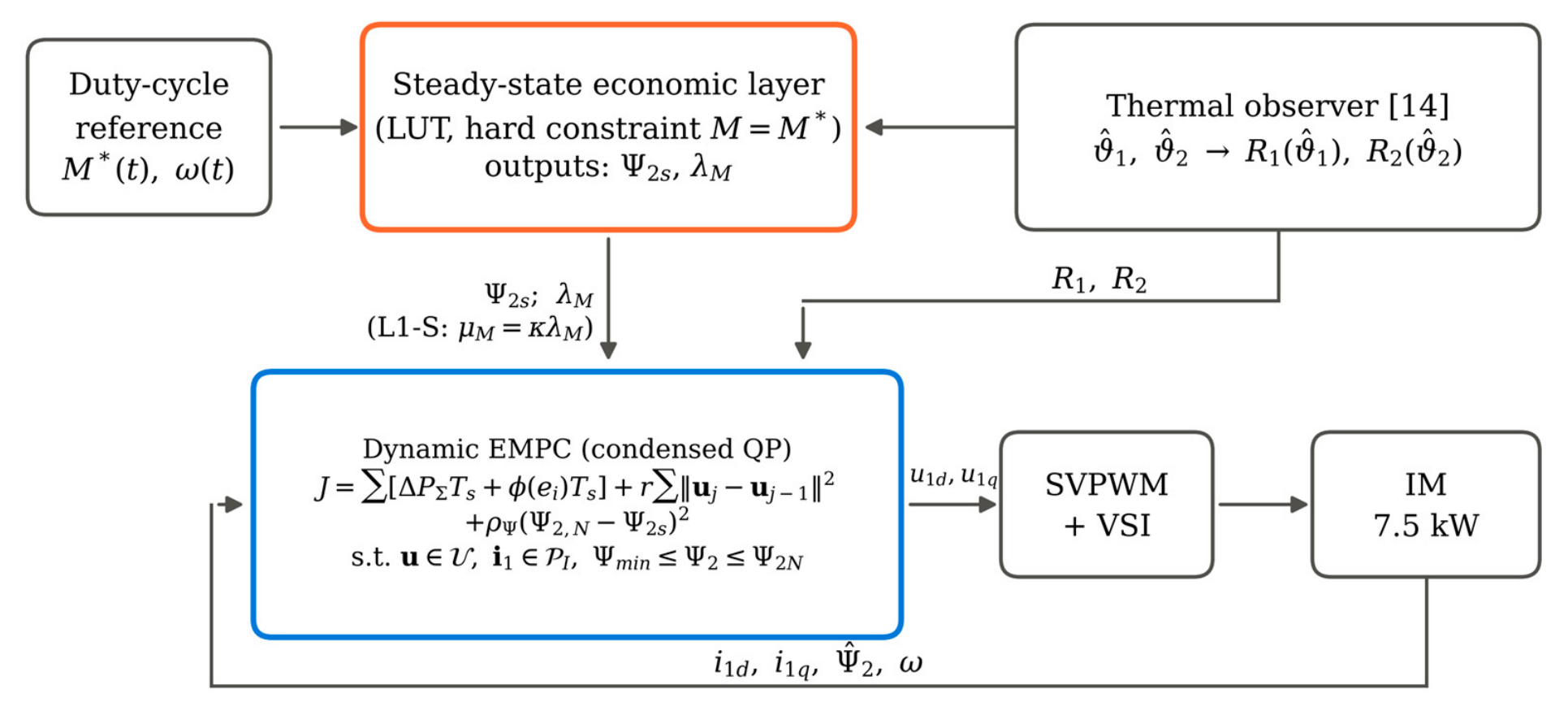
Figure 2.
Marginal loss per unit torque λM (filled contours, W/(N·m)) and loss-optimal rotor flux Ψ2s (dashed, Wb) at (a) 20 °C and (b) 115 °C. In (b), the small region above the solid line at the upper right lies beyond Mmax(ω); elsewhere Mmax exceeds 1.25MN.
Figure 2.
Marginal loss per unit torque λM (filled contours, W/(N·m)) and loss-optimal rotor flux Ψ2s (dashed, Wb) at (a) 20 °C and (b) 115 °C. In (b), the small region above the solid line at the upper right lies beyond Mmax(ω); elsewhere Mmax exceeds 1.25MN.
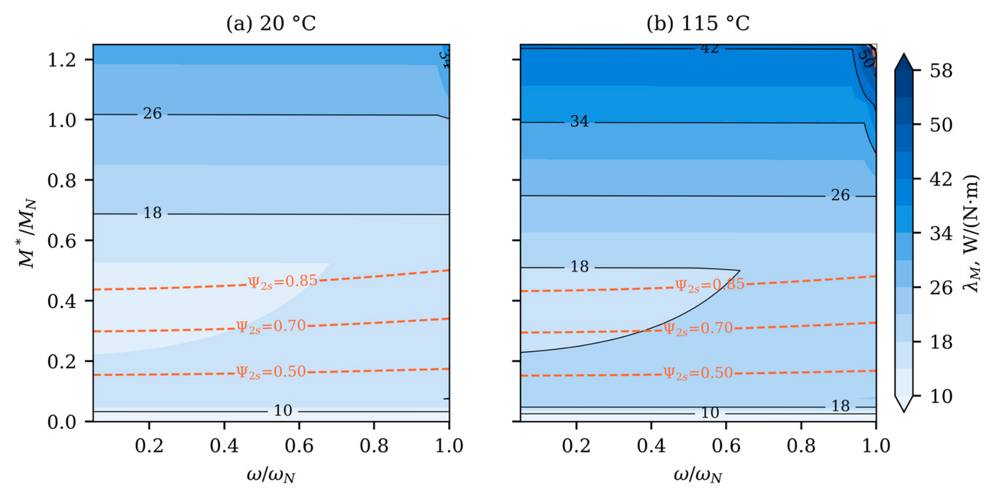
Figure 3.
Steady relative torque error versus weight. (a) Quadratic term: simulation (markers) and Proposition 1 with the flux held at Ψ2s(M*) (lines). (b) Absolute-value term, with μM normalized by the local λM; the dotted line marks μM = λM.
Figure 3.
Steady relative torque error versus weight. (a) Quadratic term: simulation (markers) and Proposition 1 with the flux held at Ψ2s(M*) (lines). (b) Absolute-value term, with μM normalized by the local λM; the dotted line marks μM = λM.
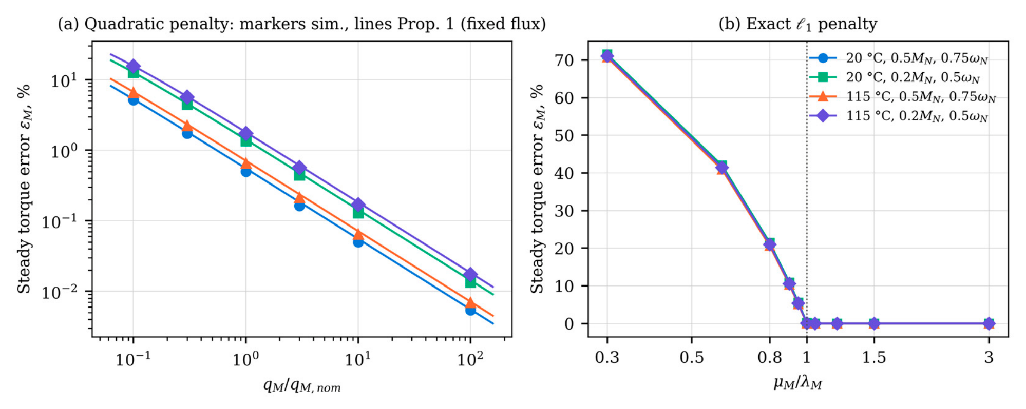
Figure 5.
Step from 0.2MN to 0.9MN at 0.75ωN, 115 °C: (a) torque and (b) rotor flux with flux reservation (preview 100 ms) for Q, L1 and L1+Q; (c) torque of L1 and Q without reservation for horizons N = 10, 20 and 40.
Figure 5.
Step from 0.2MN to 0.9MN at 0.75ωN, 115 °C: (a) torque and (b) rotor flux with flux reservation (preview 100 ms) for Q, L1 and L1+Q; (c) torque of L1 and Q without reservation for horizons N = 10, 20 and 40.
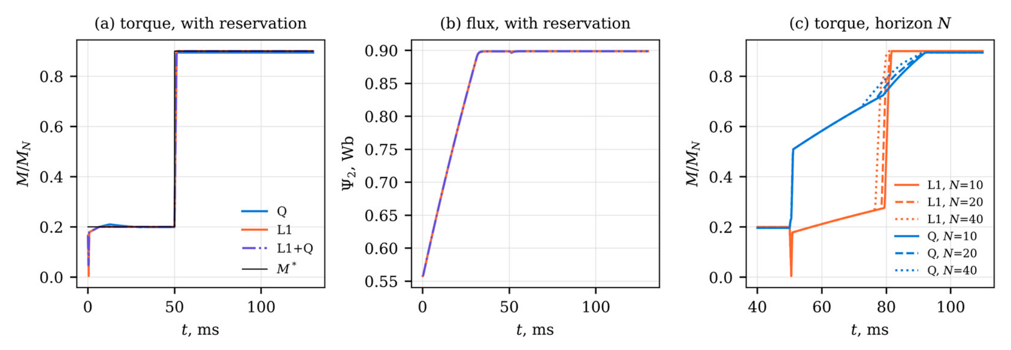
Figure 6.
Mean plateau torque error versus loss energy per delivered work, 115 °C: (a) pump cycle; (b) conveyor cycle. Q: 0.1, 1 and 10 qM,nom; L1: μM = 56.7, 68.0 and 170.1 W/(N·m), i.e., 1.0, 1.2 and 3.0 times ; L1-S: κ = 1.35. Runs without flux reservation. Errors below 10⁻³% are plotted at 10⁻³%.
Figure 6.
Mean plateau torque error versus loss energy per delivered work, 115 °C: (a) pump cycle; (b) conveyor cycle. Q: 0.1, 1 and 10 qM,nom; L1: μM = 56.7, 68.0 and 170.1 W/(N·m), i.e., 1.0, 1.2 and 3.0 times ; L1-S: κ = 1.35. Runs without flux reservation. Errors below 10⁻³% are plotted at 10⁻³%.
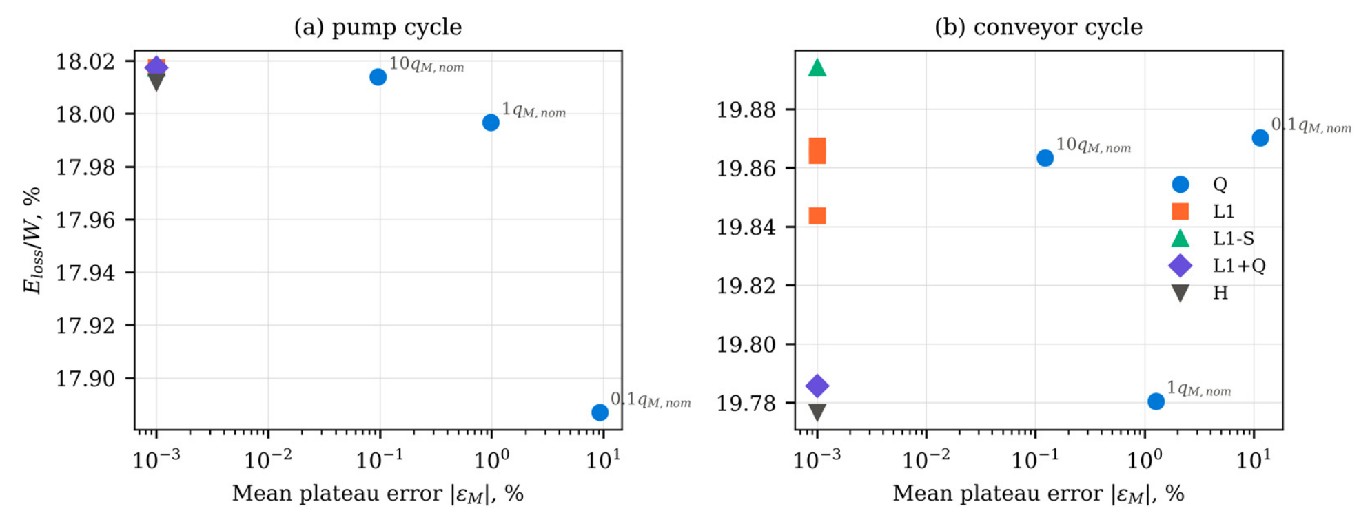
Figure 7.
(a) Monte Carlo distribution of λM for perturbed loss models (1500 samples, 18 operating points each, including rated speed) and the constant weight μM. (b) Steady torque error with mismatched R2 and Lm in the controller (100 samples per case, 115 °C): error of the true shaft torque and error of the torque estimated by the controller, for Q and L1.
Figure 7.
(a) Monte Carlo distribution of λM for perturbed loss models (1500 samples, 18 operating points each, including rated speed) and the constant weight μM. (b) Steady torque error with mismatched R2 and Lm in the controller (100 samples per case, 115 °C): error of the true shaft torque and error of the torque estimated by the controller, for Q and L1.
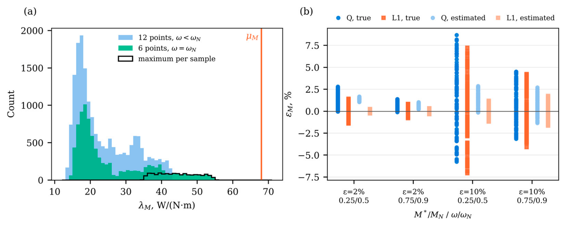
Table 1.
Parameters of the simulated drive and controller.
| Parameter | Symbol | Value | Source |
|---|---|---|---|
| Rated power, voltage, frequency | PN, UN, fN | 7.5 kW, 400 V, 50 Hz | [14], Table 3 |
| Pole pairs | zp | 2 | [14], Table 3 |
| Stator, rotor resistance at 20 °C | R1,20, R2,20 | 0.62 Ω, 0.45 Ω | [14], Table 3 |
| Stator, rotor, magnetizing inductance | L1, L2, Lm | 0.082, 0.082, 0.078 H | [14], Table 3 |
| Core-loss coefficients | kh, ke | 0.014, 4.0 × 10⁻⁴ | [14], Table 2 |
| IGBT, diode threshold voltage | UCE0, UF0 | 1.0 V, 1.1 V | [14], Table 2 |
| IGBT, diode slope resistance | rCE, rF | 25 mΩ, 20 mΩ | [14], Table 2 |
| Switching energy at 600 V, 50 A | Esw | 4.0 + 5.5 + 3.0 mJ | [14], Table 2 |
| Dc-link voltage | Ud | 540 V | [14], Section 6.1 |
| Switching frequency | fsw | 10 kHz | this study (8 kHz in [14]) |
| Temperature coefficient, stator copper | α1 | 0.00393 K⁻¹ | [14], Table 3 |
| Temperature coefficient, aluminum cage | α2 | 0.00408 K⁻¹ | this study, [26] |
| Rated rotor flux linkage | Ψ2N | 0.90 Wb | this study |
| Rated torque, speed | MN, nN | 49.2 N·m, 1457 rpm | computed |
| Rated, maximum stator current amplitude | I1N, Imax = 1.25I1N | 22.4 A, 27.9 A | computed; ratio from [14] |
| Sampling period, horizons | Ts, N, Nc | 100 µs, 10, 3 | [14], Table 3 |
| Input blocks | – | 1, 1, 8 steps | this study |
| Input-rate, terminal-flux weights | r, ρΨ | 10⁻⁶ J/V², 2 × 10⁴ J/Wb² | this study |
| Flux envelope | Ψmin, Ψmax | 0.30 Wb, 0.90 Wb | this study |
Table 2.
Torque-term weights.
| Quantity | Symbol | Value | Used in |
|---|---|---|---|
| Nominal quadratic weight | qM,nom | 52.1 W/(N·m)² | Q; quadratic part of L1+Q |
| Maximum marginal loss, hot state | 56.7 W/(N·m) | basis of μM; not used as a weight | |
| Constant absolute-value weight | 68.0 W/(N·m) | L1, L1+Q | |
| Scheduled weight | μM = κλM | κ = 1.35 | L1-S |
| Formulation | Res. | N | Infeas. QPs, % | t90, ms | IAErel of step, % | M/MN at 0.9MN | M/MN at 1.4MN, mean | Ψ2 at 1.4MN, min, Wb |
|---|---|---|---|---|---|---|---|---|
| H (fallback Q) | no | 10 | 33.5 | 36.5 | 3.50 | 0.900 | 1.266 | 0.869 |
| Q, qM,nom | no | 10 | – | 36.5 | 4.07 | 0.894 | 1.267 | 0.869 |
| Q, 10qM,nom | no | 10 | – | 15.5 | 1.31 | 0.899 | 1.050 | 0.530 |
| L1 | no | 10 | – | 31.4 | 7.56 | 0.900 | 1.297 | 0.897 |
| L1-S | no | 10 | – | 31.7 | 7.71 | 0.900 | 1.297 | 0.898 |
| L1+Q | no | 10 | – | 35.6 | 3.47 | 0.900 | 1.264 | 0.866 |
| L1+Q, 0.1qM,nom | no | 10 | – | 32.5 | 6.71 | 0.900 | 1.294 | 0.895 |
| L1+Q, 10qM,nom | no | 10 | – | 14.8 | 1.24 | 0.900 | 1.050 | 0.530 |
| Q, qM,nom | yes | 10 | – | 1.1 | 0.78 | 0.894 | 1.267 | 0.869 |
| L1 | yes | 10 | – | 1.2 | 0.15 | 0.900 | 1.297 | 0.897 |
| L1+Q | yes | 10 | – | 1.1 | 0.14 | 0.900 | 1.264 | 0.866 |
| Q, qM,nom | no | 20 | – | 35.1 | 3.97 | 0.894 | 1.256 | 0.857 |
| Q, qM,nom | no | 40 | – | 33.1 | 3.82 | 0.894 | 1.247 | 0.848 |
| L1 | no | 20 | – | 30.8 | 7.35 | 0.900 | 1.297 | 0.898 |
| L1 | no | 40 | – | 29.6 | 6.97 | 0.900 | 1.297 | 0.898 |
L1 and L1+Q use μM = 68.0 W/(N·m), L1-S uses κ = 1.35; L1+Q uses qM,nom unless stated. Res.: flux reservation with 100 ms preview. Infeas. QPs: share of infeasible QPs of H, covered by the fallback; –: not applicable. t90: time to 90% of the step from 0.2MN to 0.9MN; IAErel over 50–350 ms. H falls back to Q with qM,nom whenever its QP is infeasible.
Table 6.
Duty-cycle results.
| Formulation | Weight | Res. | ϑ, °C | Cycle | |εM|, % | IAErel, % | Eloss/W, % | Infeas. QPs, % |
|---|---|---|---|---|---|---|---|---|
| Q | 0.1qM,nom | no | 115 | pump | 9.200 | 7.61 | 17.89 | – |
| Q | qM,nom | no | 115 | pump | 0.974 | 0.79 | 18.00 | – |
| Q | 10qM,nom | no | 115 | pump | 0.096 | 0.08 | 18.01 | – |
| L1 | μM = 56.7 | no | 115 | pump | 0.000 | 0.00 | 18.02 | – |
| L1 | μM = 68.0 | no | 115 | pump | 0.000 | 0.00 | 18.02 | – |
| L1 | μM = 170.1 | no | 115 | pump | 0.000 | 0.00 | 18.02 | – |
| L1-S | κ = 1.35 | no | 115 | pump | 0.000 | 0.00 | 18.02 | – |
| L1+Q | μM = 68.0; qM,nom | no | 115 | pump | 0.000 | 0.00 | 18.02 | – |
| H | fallback qM,nom | no | 115 | pump | 0.000 | 0.00 | 18.01 | 0.0 |
| Q | qM,nom | no | 20 | pump | 0.745 | 0.59 | 14.26 | – |
| L1 | μM = 68.0 | no | 20 | pump | 0.000 | 0.00 | 14.27 | – |
| L1+Q | μM = 68.0; qM,nom | no | 20 | pump | 0.000 | 0.00 | 14.27 | – |
| Q | 0.1qM,nom | no | 115 | conveyor | 11.434 | 9.68 | 19.87 | – |
| Q | qM,nom | no | 115 | conveyor | 1.259 | 1.63 | 19.78 | – |
| Q | 10qM,nom | no | 115 | conveyor | 0.122 | 0.36 | 19.86 | – |
| L1 | μM = 56.7 | no | 115 | conveyor | 0.000 | 1.62 | 19.87 | – |
| L1 | μM = 68.0 | no | 115 | conveyor | 0.000 | 1.60 | 19.86 | – |
| L1 | μM = 170.1 | no | 115 | conveyor | 0.000 | 1.44 | 19.84 | – |
| L1-S | κ = 1.35 | no | 115 | conveyor | 0.000 | 1.75 | 19.89 | – |
| L1+Q | μM = 68.0; qM,nom | no | 115 | conveyor | 0.000 | 0.75 | 19.79 | – |
| H | fallback qM,nom | no | 115 | conveyor | 0.000 | 0.74 | 19.78 | 1.5 |
| Q | qM,nom | yes | 115 | conveyor | 1.120 | 0.95 | 19.94 | – |
| L1 | μM = 68.0 | yes | 115 | conveyor | 0.173 | 0.17 | 19.96 | – |
| L1+Q | μM = 68.0; qM,nom | yes | 115 | conveyor | 0.053 | 0.08 | 19.95 | – |
| Q | qM,nom | no | 20 | conveyor | 0.980 | 1.61 | 15.92 | – |
| L1 | μM = 68.0 | no | 20 | conveyor | 0.000 | 2.18 | 16.00 | – |
| L1+Q | μM = 68.0; qM,nom | no | 20 | conveyor | 0.000 | 0.91 | 15.91 | – |
μM in W/(N·m). Res.: flux reservation with a 100 ms preview. |εM|: mean absolute plateau error after 0.3 s of settling. Eloss/W: loss energy per delivered work. Infeas. QPs: share of infeasible QPs of H, covered by the fallback; –: not applicable.
Table 7.
Steady torque error under mismatch of R2 (±ε) and Lm (±ε/2) in the controller, 115 °C, 100 samples per case.
Table 7.
Steady torque error under mismatch of R2 (±ε) and Lm (±ε/2) in the controller, 115 °C, 100 samples per case.
| ε, % | M*/MN | ω/ωN | True error, Q | True error, L1 | Estimated error, Q | Estimated error, L1 |
|---|---|---|---|---|---|---|
| 0 | 0.25 | 0.5 | 1.36 | 0.00 | 1.36 | 0.00 |
| 0 | 0.75 | 0.9 | 0.63 | 0.00 | 0.63 | 0.00 |
| 2 | 0.25 | 0.5 | 1.33 [0.14; 2.51] | −0.02 [−1.21; 1.13] | 1.38 [1.10; 1.58] | 0.01 [−0.20; 0.17] |
| 2 | 0.75 | 0.9 | 0.57 [0.00; 1.31] | −0.06 [−0.67; 0.73] | 0.65 [0.29; 0.94] | 0.01 [−0.28; 0.26] |
| 10 | 0.25 | 0.5 | 1.24 [−4.80; 7.23] | 0.03 [−6.20; 5.78] | 1.43 [0.10; 2.44] | 0.03 [−1.00; 0.86] |
| 10 | 0.75 | 0.9 | 0.45 [−2.56; 3.96] | −0.14 [−3.44; 3.55] | 0.71 [−1.02; 2.22] | 0.07 [−1.38; 1.33] |
True error: reference minus shaft torque of the plant. Estimated error: reference minus torque computed by the controller from its own flux estimate. Values are median [5th; 95th percentile] in %.
Table 8.
Steady torque error and input activity with current-measurement noise and uncompensated dead time, 115 °C.
Table 8.
Steady torque error and input activity with current-measurement noise and uncompensated dead time, 115 °C.
| Operating point | Condition | Error Q, % | Error L1, % | Error L1+Q, % | Torque std. dev. L1, % | RMS input step Q / L1, V |
|---|---|---|---|---|---|---|
| 0.1MN, 0.5ωN | ideal | 3.69 | 0.00 | 0.00 | 0.00 | 0.0 / 0.0 |
| noise, σi = 0.1 A | 3.69 ± 0.03 | 0.15 ± 0.03 | 0.12 ± 0.03 | 2.07 | 7.2 / 15.7 | |
| noise, σi = 0.4 A | 3.66 ± 0.13 | 0.69 ± 0.13 | 0.54 ± 0.13 | 6.58 | 28.8 / 38.8 | |
| dead time 2 µs | 7.39 | 2.55 | 2.55 | 0.00 | 0.0 / 0.0 | |
| noise 0.4 A + dead time | 7.36 ± 0.12 | 4.13 ± 0.12 | 3.79 ± 0.12 | 6.51 | 28.8 / 38.3 | |
| 0.25MN, 0.5ωN | ideal | 1.36 | 0.00 | 0.00 | 0.00 | 0.0 / 0.0 |
| noise, σi = 0.1 A | 1.36 ± 0.02 | 0.03 ± 0.02 | 0.02 ± 0.02 | 1.40 | 9.4 / 17.8 | |
| noise, σi = 0.4 A | 1.35 ± 0.08 | 0.48 ± 0.08 | 0.30 ± 0.08 | 4.51 | 37.6 / 45.4 | |
| dead time 2 µs | 3.50 | 1.62 | 1.62 | 0.00 | 0.0 / 0.0 | |
| noise 0.4 A + dead time | 3.48 ± 0.08 | 2.51 ± 0.08 | 2.17 ± 0.08 | 4.47 | 37.6 / 44.7 | |
| 0.75MN, 0.9ωN | ideal | 0.63 | 0.00 | 0.00 | 0.00 | 0.0 / 0.0 |
| noise, σi = 0.1 A | 0.63 ± 0.01 | 0.01 ± 0.01 | 0.00 ± 0.01 | 0.67 | 11.4 / 18.6 | |
| noise, σi = 0.4 A | 0.86 ± 0.04 | 0.53 ± 0.04 | 0.54 ± 0.04 | 2.16 | 38.8 / 47.5 | |
| dead time 2 µs | 1.77 | 0.93 | 0.93 | 0.00 | 0.0 / 0.0 | |
| noise 0.4 A + dead time | 2.30 ± 0.04 | 1.88 ± 0.04 | 1.88 ± 0.05 | 2.04 | 33.6 / 41.6 |
Error: mean of (M* − M)/M* over the last 0.3 s of a 0.6 s run, with M the shaft torque of the plant; with noise, mean ± half-width of the 95% confidence interval over 10 noise realizations. Torque std. dev.: standard deviation of the shaft torque relative to M*. RMS input step: root mean square of ||uk − uk−1|| over the same interval. σi: standard deviation of the noise added to each measured current component. Dead time: average voltage error of 13.8 V amplitude opposite to the current vector, not compensated.
Table 9.
Numerical evidence of closed-loop convergence: linearization and small random perturbations at 36 operating points, large perturbations at 18 operating points at 115 °C.
Table 9.
Numerical evidence of closed-loop convergence: linearization and small random perturbations at 36 operating points, large perturbations at 18 operating points at 115 °C.
| Formulation | Max. ρ (36 points) | Max. τ, ms | Max. decay rate, random directions | Max. transient amplification | Converged runs | Max. final deviation |
|---|---|---|---|---|---|---|
| Q | 0.9084 | 1.04 | 0.9084 | 255 | 108/108 | 5.2 × 10⁻¹³ |
| L1 | 0.9254 | 1.29 | 0.9255 | 396 | 108/108 | 7.9 × 10⁻¹³ |
| L1+Q | 0.9254 | 1.29 | 0.9255 | 397 | 108/108 | 8.0 × 10⁻¹³ |
ρ: spectral radius of the one-step closed-loop map linearized at the equilibrium (one-sided finite differences in both directions); τ: time constant of the slowest mode, −Ts/lnρ. Decay rate: of the scaled deviation after a perturbation of norm 10−3 in a random direction, 20 directions per point; transient amplification: largest ratio of the deviation to its initial value. Large perturbations: i1d, i1q scaled by factors in [0.5, 1.5] and Ψ2 by [0.6, 1.4] (clipped to the flux envelope), 6 per operating point; converged: largest deviation from the equilibrium after 0.4 s below 10−6 in scaled units.
Table 10.
Size, active-set iterations and solution time of the condensed QP (N = 10, Nc = 3) during the sequence of Figure 4.
Table 10.
Size, active-set iterations and solution time of the condensed QP (N = 10, Nc = 3) during the sequence of Figure 4.
| Formulation | Variables | Inequality rows | Iterations, median / max | Median time, µs | 99th perc., µs | Max. time, µs |
|---|---|---|---|---|---|---|
| Q | 6 | 116 | 1 / 16 | 38 | 105 | 8126 |
| H (with fallback) | 6 | 116 + 3 eq. | 4 / 10 | 54 | 1856 | 13418 |
| L1 | 9 | 139 | 15 / 20 | 66 | 167 | 7063 |
| L1+Q | 9 | 139 | 13 / 22 | 67 | 182 | 8166 |
Iterations: number of constraints added by the Goldfarb–Idnani method, a hardware-independent measure of the work per QP. Times: Intel Xeon processor at 2.8 GHz, quadprog called from Python, 7000 QPs per formulation; they include interface overhead and are not on-target measurements. For H, an infeasible step includes the fallback solve.
Disclaimer/Publisher’s Note: The statements, opinions and data contained in all publications are solely those of the individual author(s) and contributor(s) and not of MDPI and/or the editor(s). MDPI and/or the editor(s) disclaim responsibility for any injury to people or property resulting from any ideas, methods, instructions or products referred to in the content. |
© 2026 by the authors. Licensee MDPI, Basel, Switzerland. This article is an open access article distributed under the terms and conditions of the Creative Commons Attribution (CC BY) license (http://creativecommons.org/licenses/by/4.0/).
Copyright: This open access article is published under a Creative Commons CC BY 4.0 license, which permit the free download, distribution, and reuse, provided that the author and preprint are cited in any reuse.