

Submitted:
01 November 2026
Posted:
04 November 2026
You are already at the latest version
Abstract
As climate change accelerates, spatiotemporal climate and weather data rasters are increasingly used in academic research, agriculture, infrastructure, and other disci-plines across public and private domains. Unfortunately, these raster data are often stored under numerous file types with different spatial and temporal boundaries, spa-tial reference systems, and spatial and temporal resolutions. The tools and workflows that we have are often hindered by coordinate reference system mismatches, data type mismatches, data aggregation mismatches, and other fundamental challenges. To fully harness the impacts of these data, software tools are needed that can be leveraged effi-ciently and intuitively and without a steep learning curve for the new user. In this pa-per, we introduce Spacetime, a novel programming library in Python that enables effi-cient spatiotemporal data processing, management, alignment, and analysis. Spacetime is an open-source project written in Python that provides a set of powerful functions to manipulate spatiotemporal data in a single, unified library. Spacetime’s overarching themes are simplicity and usability. However, the library does not com-promise processing speed. In our comparison, it was as fast or faster than other popu-lar Python libraries, while requiring many fewer lines of code and no external loops or control functions. We hope this library will lower the barrier of entry to scientists in fields that have not traditionally used spatiotemporal raster data but are doing so in-creasingly frequently in the current climate.
Keywords:
spatiotemporal data
; data processing
; data integration
; spatiotemporal workflow
1. Introduction
Spatiotemporal data is a critical piece of our larger data ecosystem [1,2], and a vital proposition for the utility of time geography [3,4]. Geomatics as a practical and academic area is concerned primarily with the collection, processing, and analysis of spatiotemporal data [5], and is thus essential to the discipline of time geography, a concept with far reaching practicality across almost all disciplines [6]. As we have ventured into a more democratic and ubiquitous spatiotemporal data world through concepts such as big data [7,8], crowdsourcing [9,10], and volunteered geographic information [11], the utilization of spatiotemporal data has become in many ways orphaned from the collector and its original purpose. This fundamental change has created foundational issues in data processing, most specifically in the form of mismatches of data types [12,13], coordinate reference systems [14], aggregation levels [15,16,17,18], raster grid offsets [19,20], amongst others.
Spatiotemporal data can be conceived of in many different ways. One particular approach to spatiotemporal data architectures is a layered approach managed in the form of a spatial database [21,22,23,24]. Such approaches can leverage a temporal field in the database to produce the individual layers of data at particular timestamps (Figure 1). Another approach to spatiotemporal data is found in the space-time cube [25,26]. In a space-time cube, the data for a particular variable of interest is stored in a raster brick [27], much like the bands of a raster carry aspects of color and terrain in LIDAR data (Figure 2). As such, each layer of the brick represents a different timestamp. The difference between these two formats conceptually is eminently relatable to that of the structure of wide- (space-time cube) and long-form (spatiotemporal database) data architectures [28].
Given the importance of spatiotemporal data to all sorts of fields of endeavor [31] and that many users of spatial data are not trained in computer science or geographic information science [32], software solutions that can streamline and manage these processes in an intuitive manner are of paramount importance. To that end, this paper details the Spacetime project [33,34]. The library is written in python and can be found on PyPI as “spacetimepy”. Though only the python version [34] is discussed in this paper, Spacetime is multi-language project with a beta version already written for R called “spacetimer” [33]. In the following, we will refer to the library as Spacetime, though for every language we envision a language centric naming convention.
The remainder of this paper is structured as follows: We will first discuss Spacetime’s design philosophy. We will describe the structure and API of the library. We will discuss the intended workflow of Spacetime and the role it is intended to fill. Finally, we will discuss how Spacetime was evaluated using a real-world case study and compare its performance to two other popular Python libraries.
2. Design
In this section, we dive into the design of Spacetime.
2.1. Spacetime’s Design Philosophy
Spacetime was developed around three guiding principles: reducing the time required to learn a software library, minimizing the amount of code needed to complete common operations, and maintaining computational efficiency. Although established geospatial libraries provide powerful tools for manipulating raster data, their use often requires specialized knowledge and the coordination of multiple functions or packages. These technical barriers have been identified as important limitations to the broader adoption of remote sensing and geospatial data in ecological research [35]. Furthermore, researchers have emphasized the need for greater integration of climate and ecological data, particularly when differences in spatial and temporal scales complicate their application [36].
Spacetime addresses these challenges by providing a unified interface with intuitive syntax, consistent data structures, and sensible defaults for common processing operations. Rather than developing new low-level geospatial algorithms, Spacetime builds upon established computational tools and organizes their functionality into higher-level operations. Its underlying space-time cube structure further simplifies data manipulation by treating spatial and temporal dimensions as integral components of a single dataset.
2.2. Spacetime’s Structure and API
Spacetime is an open-source software library written in Python that builds upon the Geospatial Data Abstraction Library (GDAL) for raster processing, including reprojection, resampling, and spatial alignment. The library organizes data into two primary object types: file objects, which retain raster data and associated spatial metadata, and cube objects, which represent harmonized datasets as multidimensional arrays containing spatial, temporal, and variable dimensions. This structure separates spatial preprocessing from subsequent multidimensional operations, allowing complex workflows to be performed through a consistent interface (Figure 3). Spacetime is distributed through the Python Package Index (PyPI) under the name “spacetimepy”, with source code available on GitHub [37] and complete API documentation, installation instructions, and examples hosted on the Spacetime project website [38]. The library provides functions for data ingestion, spatial alignment, temporal transformations, mathematical operations, visualization, and export (Table A1), along with object methods for accessing raster metadata and multidimensional data arrays (Table A2).
Three functions form the foundation of the Spacetime workflow: raster_align(), make_cube(), and cube_smasher(). Together, they allow users to transform heterogeneous raster files into spatially consistent datasets, organize them into multidimensional structures, and perform mathematical operations without manually managing individual raster layers. Additional functions support geographic trimming, temporal aggregation and expansion, visualization, and data export (Table 1). Each of the three primary functions is described below.
The raster_align() function standardizes the spatial properties of raster datasets, including their coordinate reference systems, pixel resolutions, and grid alignment. It accepts a Spacetime file object generated by read_data(), along with optional arguments specifying the target spatial reference system (SRS), output pixel size (resolution), resampling method (algorithm), and missing-data value (noneVal). Supported resampling methods include nearest neighbor, bilinear interpolation, Lanczos, and several statistical aggregation methods. Additionally, the function allows users to crop these data either by specifying a bounding box using the union or intersection arguments or by passing the function a shape file.
The make_cube() function converts spatially aligned file objects into multidimensional space-time cubes that serve as the primary analytical structure within Spacetime. Users specify how individual raster files and their constituent bands should be organized along temporal or variable dimensions using the organizeFiles and organizeBands arguments. Additional arguments allow users to assign variable names (varNames), define a temporal sequence (timeObj), and control whether data are accessed through lazy loading or in-memory arrays (inMemory). The resulting cube object provides a consistent representation of spatial coordinates, time, and environmental variables, enabling subsequent transformations and data extraction.
The cube_smasher() function performs mathematical and user-defined operations on one or more multidimensional datasets while preserving the structure of the resulting space-time cube. Inputs may include Spacetime cube objects, NumPy arrays, and scalar values, which can be combined through a mathematical expression supplied as a character string (eq) or processed using a user-defined function (function). An optional parentCube argument identifies the reference cube whose structure and metadata guide reconstruction of the output. The function returns a new cube object containing the calculated values, allowing operations such as combining environmental variables, calculating anomalies, and applying mathematical transformations without manually iterating through raster layers.
2.3. Spacetime’s Intended Workflow
Consider a scenario in which a researcher wishes to examine how land use, soil moisture, and vegetation cover influence species distributions across a geographic region. These datasets may originate from different sources and differ in file format, coordinate reference system, spatial resolution, geographic extent, and temporal resolution. Spacetime provides a streamlined workflow for integrating these disparate datasets (Figure 3). The workflow begins with the importing of a list of raster files into a Spacetime file object using read_data(). These objects retain the underlying data and spatial metadata and can be queried using any of the spacetime query methods (Table A2) returning a list of outputs (one for each raster). However, the object is not yet a unified cube. This interim stage allows for the user to easily see the attributes of each raster and make a decision about how to merge them. When a decision is reached, raster_align() is used to establish common projections, pixel sizes, and geographic boundaries.
Once spatially aligned, the data set is organized into a multidimensional space-time cube using make_cube(). This function takes in the desired orientation incorporating spatial coordinates, temporal information, and environmental variables into a common structure. Users can then manipulate the temporal dimension through aggregation, expansion, or selection using functions such as scale_time(), expand_time(), and select_time(), while cube_smasher() takes as input spacetime objects, arrays, user defined equations, and functions and conducts operations within and between datasets. Finally, processed cubes can be visualized, converted to tabular formats, or exported for further analysis. By organizing these operations into a sequential workflow, Spacetime allows researchers to integrate heterogeneous environmental datasets without manually managing individual raster layers, temporal loops, or multiple software libraries.
2.4. Evaluating Spacetime’s Performance and Comparison with Existing Libraries.
To evaluate Spacetime’s performance and compare its speed and usability to other libraries, we conducted a case study where daily future weather data was computed with a future climatology and past daily weather data using the delta method [39,40]. This approach allows researchers to select a historical weather year exhibiting characteristics of interest, such as unusually high temperatures, prolonged drought, or extreme precipitation, and evaluate how those patterns might manifest under future climate conditions. Monthly anomalies are calculated as the difference between projected future and historical baseline climatologies and subsequently applied to the corresponding days of the selected historical year. For temperature, these anomalies represent absolute changes in monthly mean temperature, whereas precipitation can be adjusted using proportional differences between future and baseline conditions [39].
The delta method preserves the temporal structure of the selected historical year, including the sequence of daily weather events, short-term variability, and relative timing of extremes, while modifying their magnitudes according to projected climatic changes [40]. For temperature, the projected daily value was calculated as:
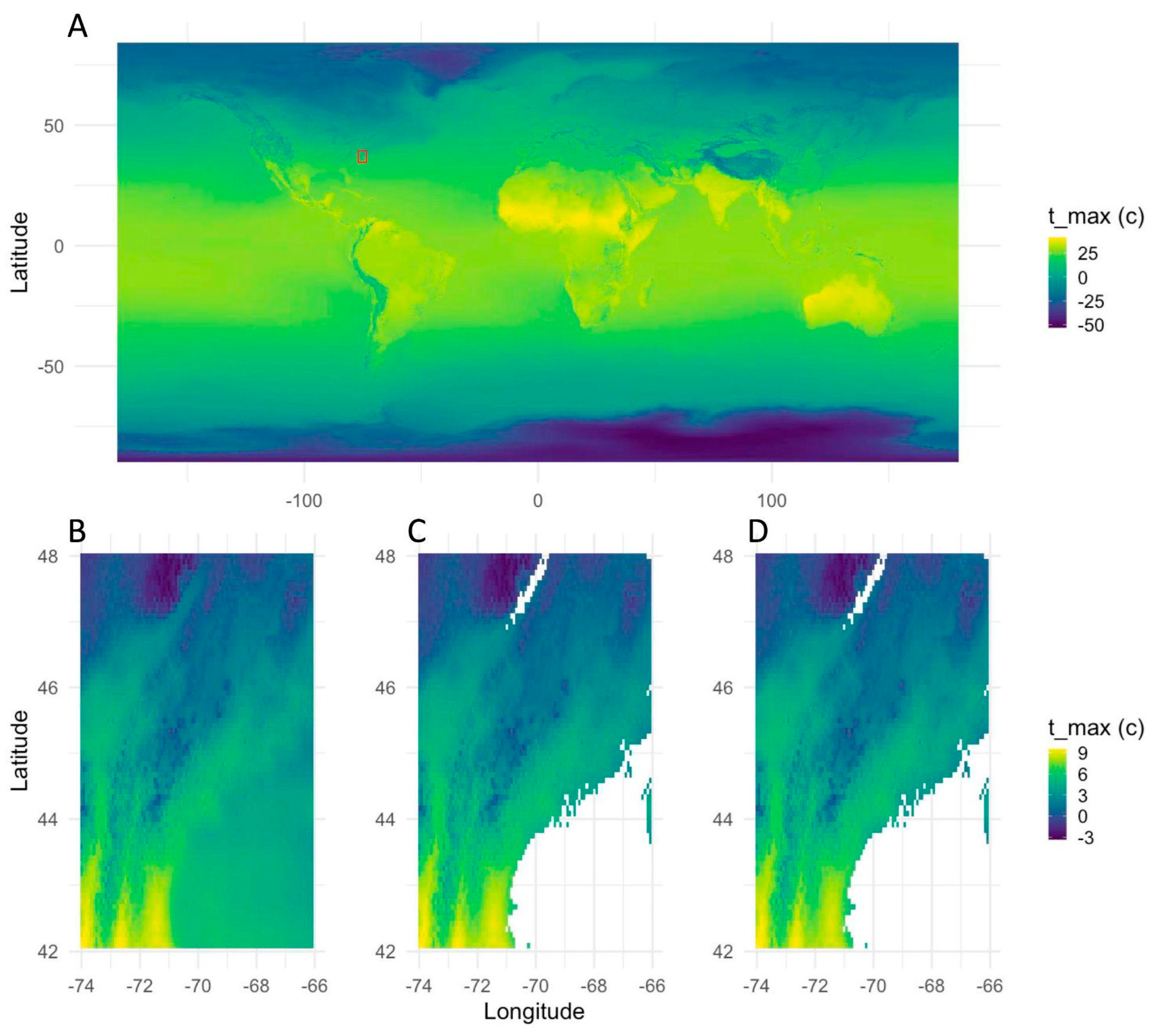
where is the difference between future and historical monthly mean temperatures for month . By retaining the observed daily sequence, this approach enables investigation of how particular historical weather conditions might affect ecological processes under future climates (Figure 4). With the framework for the case study in place, we first examined how runtime and memory consumption scaled across spatial resolutions and resampling methods comparing performance to GDAL, Spacetime’s underlying engine to ensure Spacetime’s overhead stayed low. We then compared execution times and the lines of code required to complete an equivalent workflow across Spacetime, GDAL, and Rasterio. Together, these comparisons assess whether Spacetime can simplify complex spatiotemporal data processing without compromising computational performance.
3. Materials and Methods
All computational analyses and performance benchmarks were conducted on a first-generation Apple Mac Studio (2022), equipped with an Apple M1 Max processor (10-core CPU; 8 performance and 2 efficiency cores) and 32 GB of unified memory, running macOS. Raster processing was done in Python (v3.9.5). Graphics were created in R (v4.2.3) using ggplot2 (v4.0.1). All scripts used in the case study and computational benchmarking are available in a separate public github repository [41]. The case study combined projected monthly climatologies from CHELSA 2020–2040, SSP5-8.5 [42] with historical daily max temperature data from 2019 sourced from Daymet [43].
3.1. Spacetime’s Performance.
To evaluate computational performance across spatial scales, we conducted a series of benchmarking sweeps comparing Spacetime (v0.1.7) and GDAL (v3.2.1) across a range of output raster resolutions and resampling methods. The processing operation used for these benchmarks was drawn from the climate-data case study described in detail in Section 3.2. Output pixel sizes were systematically varied across five orders of magnitude, from fine to coarse spatial resolutions. Three sequences of pixel sizes were evaluated, using bases of 1, 5, and the native pixel resolution of the original raster (0.0083 degrees). These independent sequences were intended to identify potential resolution-dependent scaling artifacts that might otherwise be obscured by testing a single progression of pixel sizes. Each sequence was evaluated using three resampling methods: nearest neighbor, Lanczos, and average resampling.
For each combination of output pixel size, resampling method, and software library, we recorded computational runtime (seconds) and memory consumption (GB). Runtime was evaluated on a logarithmic scale to accommodate differences in execution time spanning several orders of magnitude. Memory consumption was compared across the same combinations to assess how resource requirements changed with output resolution and resampling algorithm. All comparisons used the same source datasets and processing operation, allowing differences in computational performance to be evaluated across equivalent spatial transformations. Together, these benchmarks were designed to characterize the scalability of Spacetime relative to GDAL and determine whether its higher-level interface introduced computational overhead across different spatial resolutions and resampling methods.
3.2. Future Daily Climatology Case Study and Software Comparison.
We generated daily weather projections under future climate conditions using the delta method, a climate-change scenario technique that combines observed historical weather sequences with projected changes in long-term climatological conditions [39,40]. To demonstrate this approach, we combined historical daily maximum-temperature observations from Daymet (2019) with projected monthly maximum-temperature climatologies from CHELSA (2030–2040). The CHELSA dataset consisted of 12 monthly GeoTIFF rasters with global coverage, a geographic coordinate reference system (EPSG:4326), a spatial resolution of 0.008333°, and dimensions of 43,200 × 20,880 pixels. The Daymet dataset contained 365 daily observations covering North America, with a spatial resolution of 1,000 m, a projected coordinate reference system (EPSG:9122), and dimensions of 7,814 × 8,075 pixels. These datasets differed substantially in geographic extent, spatial projection, resolution, and temporal structure, providing a representative test of heterogeneous spatiotemporal data integration.
The processing workflow involved spatially aligning the historical Daymet observations with the CHELSA climatology, including reprojection, resampling, and geographic subsetting to a common grid. The aligned daily observations were aggregated into 12 monthly mean maximum-temperature rasters, which were subtracted from the corresponding future CHELSA climatologies to calculate monthly temperature anomalies. These anomalies were expanded to daily resolution by assigning each monthly anomaly to all corresponding days of the year. The resulting daily anomalies were added to the aligned 2019 Daymet observations, producing 365 projected daily maximum-temperature rasters representing 2019-like weather conditions under the 2030–2040 future climatology (Figure 4). This workflow required the integration of spatial and temporal transformations, raster arithmetic, and multidimensional data management.
To evaluate computational performance and programming complexity, the complete case-study workflow was independently implemented using GDAL (v3.2.1), Rasterio (v1.2.6), and Spacetime (v0.1.7) in Python. Each implementation used identical input datasets and target spatial and temporal parameters, and the complete workflow was executed 16 times per library. Benchmarks excluded the initial reading of source data from disk but included opening the data within each library's respective data structures, all subsequent spatial and temporal operations, and writing the final output to disk. Execution times were recorded for each replicate, and programming complexity was evaluated by comparing the number of lines of code required to complete the workflow.
4. Results
4.1. Spacetime’s Performance.
Computational runtime increased substantially as output pixel size decreased for both GDAL and Spacetime (Figure 5). Across nearest-neighbor, Lanczos, and average resampling methods, both libraries exhibited similar scaling patterns, with execution times increasing several orders of magnitude at the finest spatial resolutions. At intermediate resolutions, GDAL and Spacetime generally completed operations in comparable times, although Spacetime exhibited longer runtimes at some of the coarsest resolutions, particularly with Lanczos resampling. Runtime was relatively consistent across the three pixel-size sequences (bases of 1, 5, and native raster resolution), suggesting that the observed scaling patterns were primarily driven by output resolution rather than the sequence of pixel sizes selected.
Memory consumption differed more substantially between libraries (Figure B1). GDAL generally exhibited lower memory usage, ranging from approximately 15 to 22 GB, whereas Spacetime remained near 24–26 GB across most resolutions and resampling methods. GDAL memory consumption increased with coarser output resolutions in some configurations, particularly for the base-5 and native-resolution sequences, while Spacetime memory requirements were comparatively stable. Memory usage showed little variation among the three resampling methods within each library. Together, these results indicate that Spacetime maintained broadly comparable runtime scaling to GDAL across spatial resolutions and resampling algorithms, although with greater and more consistent memory requirements.
4.2. Future Daily Climatology Case Study and Software Comparison.
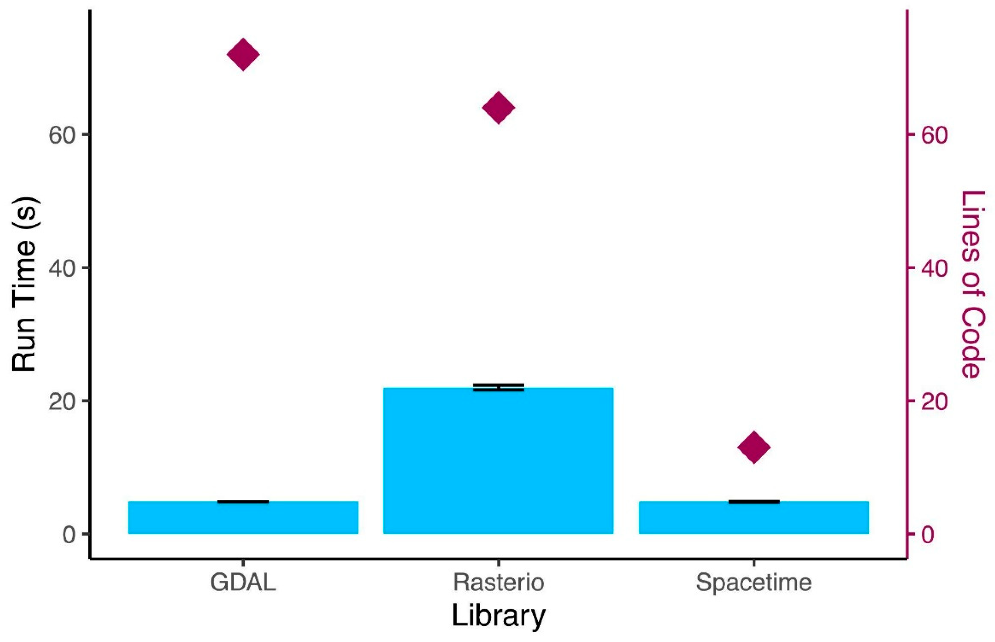
The delta-method case study revealed substantial differences in computational performance among the three libraries (Figure 6, Figure B2). Across 16 replicate executions of the complete workflow, GDAL had an average execution time of 4.84 seconds (sd = 0.029) and Spacetime’s average was 4.91 seconds (sd = 0.03). GDAL and Spacetime exhibited nearly identical mean execution times of approximately 5 seconds whereas Rasterio required an average of 22 seconds (sd = 0.367). Thus, Spacetime completed the workflow approximately four times faster than Rasterio while maintaining performance comparable to GDAL. Execution times showed relatively little variability among repetitions, with particularly small standard deviations for GDAL and Spacetime. These results indicate that Spacetime's higher-level interface did not impose a substantial runtime penalty relative to GDAL for this workflow.
Differences in programming complexity were more pronounced than differences in execution time. Implementing the complete workflow required 72 lines of code using GDAL and 64 lines using Rasterio, compared with only 13 lines using Spacetime (Figure 6). This represents an approximately 80% reduction in code length relative to the other two libraries. The reduction was achieved while performing the same spatial alignment, temporal aggregation, anomaly calculation, temporal expansion, and output operations. Collectively, these results demonstrate that Spacetime substantially reduced the programming effort required to integrate heterogeneous spatiotemporal datasets while retaining computational performance comparable to GDAL and substantially exceeding that of Rasterio in the case-study workflow.
5. Discussion
Spacetime demonstrates that complex spatiotemporal raster processing can be simplified without substantially compromising computational performance. Across spatial resolution sweeps, Spacetime exhibited runtime scaling comparable to GDAL, although with greater memory requirements. In the climate projection case study, Spacetime completed the workflow at approximately the same time as GDAL and substantially faster than Rasterio, while requiring approximately 80% fewer lines of code. These results suggest that higher-level abstractions can reduce programming complexity without introducing substantial computational overhead. By integrating spatial and temporal operations into a unified workflow, Spacetime provides an accessible alternative to manually coordinating multiple geospatial libraries.
The value of this approach extends beyond computational efficiency. As high-resolution environmental datasets become increasingly available, researchers must integrate information across different spatial and temporal scales, often requiring specialized programming expertise. Previous studies have identified technical complexity, limited training, and fragmented software tools as barriers to incorporating geospatial data into ecological research [35,44]. Spacetime addresses these challenges through intuitive syntax, consistent data structures, and streamlined operations. Although the benchmarks presented here demonstrate its potential for climate-data processing, the same framework could support applications in agriculture, ecology, hydrology, and other disciplines that rely on heterogeneous spatiotemporal datasets.
Future development will focus on expanding the R implementation of Spacetime and establishing a sustainable open-source community around the platform. R is widely used in ecological research, and its extensive ecosystem of spatial packages, including raster and terra, demonstrates the importance of accessible geospatial tools within this community [45,46]. Extending Spacetime's unified workflow to R would broaden accessibility while maintaining consistency between programming environments. Parallel efforts will emphasize documentation, tutorials, community contributions, and interoperability with established geospatial libraries. Together, these developments aim to establish Spacetime as a sustainable, community-supported resource for efficient and reproducible spatiotemporal data analysis.
As Spacetime is fundamentally built to address rasters and spacetime cubes, its status as open source provides direct opportunity for integrating something missing from a modern GIS: raster reasoning, as well as application areas that are perhaps foreign to certain disciplines. Modern geospatial tools often do not integrate core aspects of spatial, temporal, or spatiotemporal reasoning within them. While most geographic information systems (GIS) software includes concepts such as the Clementini operators [47], they do not include support for insights pertaining to conceptual neighborhood graphs that invoke similarity between those operators [48,49]. Moreover, the Clementini operators are only implemented for vectorized data, leaving discretized relation sets (e.g., [50,51,52]) outside the purview of cognitively-simplified spatial query systems. Similarly, event detection concepts common to industrial applications such as Shewhart control charts [53,54] within the statistical process control framework [55] are not found in many application spaces that could benefit from them. Approaching these types of concepts would provide opportunities for novel applications within data-forward communities with spatial data as a fundamental piece. These are not just software issues; the research community only recently began to approach theoretical work upon temporal concepts in discretized data [56,57], concepts fundamental to a spatiotemporal analytics system that has the capacity to be more human-intuitive [58,59,60].
Author Contributions
Conceptualization, P.B., M.D., S.M., M.K., N.G., B.J.M.; methodology, P.B, M.D., B.J.M.; software, P.B., Q.D.; validation, P.B.; formal analysis, P.B.; investigation, M.D. ,N.G. ,B.J.M.; resources, P.B., Q.D.; data curation, P.B.; writing—original draft preparation, P.B., M.D..; writing—review and editing, P.B., M.D., S.M., B.P.M.,M.K., N.G., B.J.M.; visualization, P.B., M.D.; supervision, P.B.; project administration, B.J.M.; funding acquisition, M.D., N.G., B.J.M. All authors have read and agreed to the published version of the manuscript.
Funding
This research was funded by US National Science Foundation, grant numbers 2019470 and 2218063.
Data Availability Statement
No new data was generated in this study.
Acknowledgments
The authors gratefully acknowledge other members of the BARRACUDA NSF EPSCoR team (L. Kate Corlew, Leo Edmonston-Cyr, Elizabeth Espinosa Uquillas, Brendan Hall, Meredith Niles, Hossein Sabzian Papi, Timothy Waring), grant external advisory team members (Kevin Gardner, Daniel Gruner, Heather McInnis, Laura Schmitt-Olabassi), Spacetime hack-a-thon participants, and Spacetime training session participants for their valuable contributions to the design and scope of Spacetime.
Conflicts of Interest
The authors declare no conflicts of interest.
Appendix A

Table A1.
Core functions of the Spacetime library. Functions are grouped into four categories: input, scaling, operations, and output. Descriptions summarize the primary functionality of each operation for importing, harmonizing, manipulating, and exporting spatiotemporal raster data.
Table A1.
Core functions of the Spacetime library. Functions are grouped into four categories: input, scaling, operations, and output. Descriptions summarize the primary functionality of each operation for importing, harmonizing, manipulating, and exporting spatiotemporal raster data.
| Category | Function | Description |
| Input | read_data() | Reads raster data as a list of file names/paths. |
| load_cube() | Loads a previously created cube object (.nc4 file). | |
| cube_time() | Creates a time vector to add to a new Spacetime dataset. | |
| Scale | raster_align() | Aligns files to a common pixel size and spatial reference system and crops them. |
| scale_time() | Scales the time dimension using a selected statistic and interval. | |
| expand_time() | Expands a coarse time domain into a finer time domain. | |
| Operations | select_time() | Selects specified times (dates, days, months, etc.). |
| cube_smasher() | Performs mathematical or function-based operations between cubes. | |
| plot_cube() | Plots cubes in interactive web-based interfaces. | |
| cube_to_dataframe() | Converts a cube into a pandas dataframe. | |
| Output | make_cube() | Converts raster files into a cube object and writes it to disk. |
| write_csv() | Writes a Spacetime dataframe as a .csv file. |
Table A2.
Spacetime object methods and metadata access. Methods available for retrieving spatial, temporal, and structural information from Spacetime objects, including coordinate reference systems, raster dimensions, geographic coordinates, temporal attributes, and underlying data arrays.
Table A2.
Spacetime object methods and metadata access. Methods available for retrieving spatial, temporal, and structural information from Spacetime objects, including coordinate reference systems, raster dimensions, geographic coordinates, temporal attributes, and underlying data arrays.
| Method | Description |
| .get_GDAL_data() | Retrieves the original GDAL object. |
| .get_epsg_code() | Retrieves the EPSG code used in the object. |
| .get_units() | Retrieves the pixel units of current spatial reference system. |
| .get_UL_corner() | Retrieves the upper-left corner coordinates. |
| .get_band_number() | Retrieves the number of bands in the dataset. |
| .get_time() | Retrieves the object’s time vector. |
| .get_dims() | Retrieves the x and y dimensions. |
| .get_nodata_value() | Retrieves the no-data value. |
| .get_data_array() | Retrieves the data as an xarray. |
| .get_lat() | Retrieves the latitude vector. |
| .get_lon() | Retrieves the longitude vector. |
| .get_var_names() | Retrieves the variable names in higher-dim datasets. |
| .get_file_size() | Retrieves the original datasets’ file sizes on disk. |
| .get_spatial_ref() | Retrieves the full spatial reference system. |
| Method | Description |
| .get_GDAL_data() | Retrieves the original GDAL object. |
| .get_epsg_code() | Retrieves the EPSG code used in the object. |
| .get_units() | Retrieves the pixel units of current spatial reference system. |
| .get_UL_corner() | Retrieves the upper-left corner coordinates. |
| .get_band_number() | Retrieves the number of bands in the dataset. |
| .get_time() | Retrieves the object’s time vector. |
| .get_dims() | Retrieves the x and y dimensions. |
| .get_nodata_value() | Retrieves the no-data value. |
| .get_data_array() | Retrieves the data as an xarray. |
| .get_lat() | Retrieves the latitude vector. |
| .get_lon() | Retrieves the longitude vector. |
| .get_var_names() | Retrieves the variable names in higher-dim datasets. |
| .get_file_size() | Retrieves the original datasets’ file sizes on disk. |
| .get_spatial_ref() | Retrieves the full spatial reference system. |
Appendix B
Figure B1.
Memory consumption across spatial resolutions and resampling methods. Memory usage (GB) for GDAL and Spacetime across a range of output pixel sizes and three resampling methods (nearest neighbor, Lanczos, and average). Pixel sizes were varied across orders of magnitude using sequences based on 1, 5, and the native resolution of the original raster to evaluate scaling behavior and identify potential resolution-dependent artifacts.
Figure B1.
Memory consumption across spatial resolutions and resampling methods. Memory usage (GB) for GDAL and Spacetime across a range of output pixel sizes and three resampling methods (nearest neighbor, Lanczos, and average). Pixel sizes were varied across orders of magnitude using sequences based on 1, 5, and the native resolution of the original raster to evaluate scaling behavior and identify potential resolution-dependent artifacts.
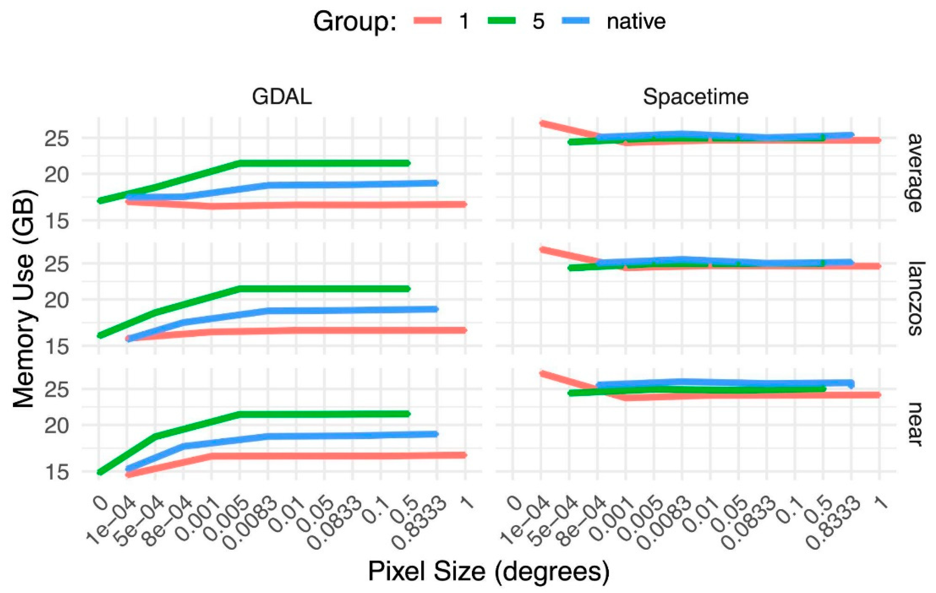
Figure B2.
Spatial processing of temperature raster data using Spacetime. Representative maximum-temperature rasters from the first time slice of each cube illustrating successive stages of the processing workflow described in section 2.2. A) The original global temperature dataset B) Geographic cropping and spatial resampling. C) The calculated deltas. D) The final rescaled future daily climate raster.
Figure B2.
Spatial processing of temperature raster data using Spacetime. Representative maximum-temperature rasters from the first time slice of each cube illustrating successive stages of the processing workflow described in section 2.2. A) The original global temperature dataset B) Geographic cropping and spatial resampling. C) The calculated deltas. D) The final rescaled future daily climate raster.
References
- Shekhar, S.; Jiang, Z.; Ali, R.; Eftelioglu, E.; Tang, X.; Gunturi, V.; Zhou, X. Spatiotemporal data mining: a computational perspective. International Journal of Geoinformation 2015, 4(4), 2306-2338. [CrossRef]
- Alam, M.; Torgo, L.; Bifet, A. A survey on spatio-temporal data analytics systems. ACM Computing Surveys 2022, 54(10s), 1-38. [CrossRef]
- Hagerstrand, T. What about people in regional science. In Transport Sociology: Social Aspects of Transport Planning, 1970, 143-158.
- Pred, A. The choreography of existence: comments on Hagerstrand’s time-geography and its usefulness. Economic Geography 1977, 53(2), 207-221. [CrossRef]
- Li, D.; Shen, X.; Wang, L. Connected geomatics in the big data era. International Journal of Digital Earth 2018, 11(2), 139-153. [CrossRef]
- Winter, S.; Yin, Z. The elements of probabilistic time geography. Geoinformatica 2011, 15(3), 417-434. [CrossRef]
- Cuzzocrea, A. Provenance research issues and challenges in the big data era. In IEEE 39th Annual Computer Software and Applications Conference, 2015, 684-686.
- Lee, J.; Kang, M. Geospatial big data: challenges and opportunities. Big Data Research 2015, 2(2), 74-81. [CrossRef]
- Heipke, C. Crowdsourcing geospatial data. ISPRS Journal of Photogrammetry and Remote Sensing 2010, 65(6), 550-557. [CrossRef]
- Tong, Y.; Zhou, Z.; Zeng, Y.; Chen, L.; Shahabi, C. Spatial crowdsourcing: a survey. The VLDB Journal 2020, 29(1), 217-250. [CrossRef]
- Goodchild, M. Citizens as sensors: the world of volunteered geography. GeoJournal 2007, 69(4), 211-221. [CrossRef]
- Dube, M.; Barrett, J.; Egenhofer, M. From metric to topology: determining relations in discrete space. In International Conference on Spatial Information Theory, Springer: Cham, Germany, 2015, pp. 151-171.
- Dube, M.; Hall, B.; Thibeau, T. Big data, crowdsourcing, and volunteered geographic information challenge core conceptual neighborhood graph assumptions. Geomatics 2026, 6(3), 64. [CrossRef]
- Xiong, D.; Lin, H. Spatial data handling for ITS: perspective, issues, and approaches. GeoInformatica 2000, 4(2), 215-230. [CrossRef]
- Clark, W.; Avery, K. The effects of data aggregation in statistical analysis. Geographical Analysis 1976, 8(4), 428-438. [CrossRef]
- Wu, J. Effects of changing scale on landscape pattern analysis: scaling relations. Landscape Ecology 2004, 19(2), 125-138. [CrossRef]
- Indulska, M.; Orlowska, M. On aggregation issues in spatial data management. In Thirteenth Australasian Database Conference, 2002, pp. 75-84.
- Goovaerts, P. Geostatistical analysis of health data with different levels of spatial aggregation. Spatial and Spatio-Temporal Epidemiology 2012, 3(1), 83-92. [CrossRef] [PubMed]
- Avelino, A.; Baylis, K.; Honey-Roses, J. Goldilocks and the raster grid: selecting scale when evaluating conservation programs. PLoS One 2016, 11(12), e0167945. [CrossRef] [PubMed]
- Zhao D.; Fu, F.; Lu, H.; Yang, C. Study on the effect of raster center coordinate offset on urban DEM in surface catchment simulation. Journal of Geo-Information Science 2026, 28(4), 957-970.
- Yuan, M. Use of a three-domain representation to enhance GIS support for complex spatiotemporal queries. Transactions in GIS 1999, 3(2), 137-159. [CrossRef]
- Claramunt, C.; Jiang, B. An integrated representation of spatial and temporal relationships between evolving regions. Journal of Geographical Systems 2001, 3(4), 411-428. [CrossRef]
- Huang, B.; Claramunt, C. STOQL: an ODMG-based spatio-temporal object model and query language. In Advances in Spatial Data Handling: 10th International Symposium on Spatial Data Handling. Springer: Berlin, 2002, pp. 225-237.
- Huang, B.; Claramunt, C. Spatiotemporal data model and query language for tracking land use change. Transportation Research Record 2005, 1902(1), 107-113. [CrossRef]
- Kraak, M. The space-time cube revisited from a geovisualization perspective. In 21st International Cartographic Conference. International Cartographic Association, 2003, pp. 1988-1996.
- Deng, Z.; Huang, J.; Ruan, C.; Li, J.; Gao, S.; Cai, Y. Volume-based space-time cube for large-scale continuous spatial time series. IEEE Transactions on Visualization and Computer Graphics 2025, 31(10), 7019-7033. [CrossRef] [PubMed]
- Lamigueiro, O. Spatiotemporal raster data. In Displaying Time Series, Spatial, and Space-Time Data with R. Chapman and Hall, 2025, pp. 249-265.
- Walther, J.; Hecht, M.; Nagengast, B.; Zitzmann, S. To be long or to be wide: how data format influences convergence and estimation accuracy in multilevel structural equation modeling. Structural Equation Modeling: A Multidisciplinary Journal 2024, 31(5), 759-774. [CrossRef]
- Nhat Hai, P.; Poncelet, P.; Teisseire, M. Get_move: an efficient and unifying spatio-temporal pattern mining algorithm for moving objects. In International Symposium on Intelligent Data Analysis. Springer: Berlin, 2012, pp. 276-288.
- Wang, D; Cao, Z.; Wu, M.; Wan, B.; Wu, S.; Zhang, Q. Articulating environmental sustainability dynamics with space-time cube. Ecological Informatics 2024, 83, 102833. [CrossRef]
- Yang, C.; Clarke, K.; Shekhar, S.; Tao, C. Big spatiotemporal data analytics: a research and innovation frontier. International Journal of Geographical Information Science 2020, 34(6), 1075-1088. [CrossRef]
- Rickles, P.; Ellul, C.; Haklay, M. A suggested framework and guidelines for learning GIS in interdisciplinary research. Geo: Geography and Environment 2017, 4(2), e00046. [CrossRef]
- Burnham, P.; Dube, M.; Dubois, Q.; Gotelli, N.; McGill, B. SpaceTime: a package for cleaning and analyzing spatiotemporal data in R. https://github.com/alexburn17/spacetime_r.
- Burnham, P.; Dube, M.; Dubois, Q.; Gotelli, N.; McGill, B. SpaceTime: a library for cleaning and analyzing spatiotemporal data in Python. https://github.com/alexburn17/spacetime_python.
- Pettorelli, N.; Laurence, W.; O’Brien, T.; Wegmann, M.; Nagendra, H.; Turner, W. Satellite remote sensing for applied ecologists: opportunities and challenges. Journal of Applied Ecology 2014, 51(4), 839-848. [CrossRef]
- Baker, D.; Hartley, A.; Pearce-Higgins, J.; Jones, R.; Willis, S. Neglected issues in using weather and climate information in ecology and biogeography. Diversity and Distributions 2017, 23(3), 329-340. [CrossRef]
- Burnham, P.A. spacetimepy 0.1.7. 2026. https://pypi.org/project/spacetimepy/.
- Burnham, P.A. The Spacetime project. 2023. https://alexburn17.github.io/Theme3_LabNotebook/description.html.
- Hay, L.; Wilby, R.; Leavesley, G. A comparison of delta change and downscaled GCM scenarios for three mountainous basins in the United States. Journal of American Water Resources Association 2000, 36(2), 387-397. [CrossRef]
- Belcher, S.; Hacker, J.; Powell, D. Constructing design weather data for future climates. Building Services Engineering Research and Technology 2005, 26(1), 49-61. [CrossRef]
- Burnham, P. A. 2026. barra_python: Code and computational workflows for the Spacetime case study and benchmarking analyses. GitHub. https://github.com/alexburn17/barra_python.
- Karger, D. N., Y. Chauvier, and N. E. Zimmermann. 2023. chelsa-cmip6 1.0: A Python package to create high resolution bioclimatic variables based on CHELSA ver. 2.1 and CMIP6 data. Ecography 2023:e06535. [CrossRef]
- Thornton, M. M., R. Shrestha, Y. Wei, P. E. Thornton, and S.-C. Kao. 2020. Daymet: Daily surface weather data on a 1-km grid for North America, Version 4. ORNL Distributed Active Archive Center, Oak Ridge, Tennessee, USA. [CrossRef]
- Lortie, C.; Braun, J.; Filazzola, A.; Miguel, F. A checklist for choosing between R packages in ecology and evolution. Ecology and Evolution 2020, 10(3), 1098-1105. [CrossRef] [PubMed]
- Lai, J.; Lortie, C.; Muenchen, R.; Yang, J.; Ma, K. Evaluating the popularity of R in ecology. Ecosphere 2019, 10(1), e02567. [CrossRef]
- Hijmans, R.; Brown, A.; Barbosa, M.; Cordano, E.; Dyba, K. terra: spatial data analysis. R package version 1.9-55, https://github.com/rspatial/terra.
- Clementini, E.; Sharma, J.; Egenhofer, M. Modelling topological spatial relations: strategies for query processing. Computers and Graphics 1994, 18(6), 815-822. [CrossRef]
- Freksa, C. Temporal reasoning based on semi-intervals. Artificial Intelligence 1992, 54(1-2), 199-227. [CrossRef]
- Dube, M.; Hall, B. Conceptual neighborhood graphs: event detectors, data relevancy, and language translation. In Geography According to Foundation Models. IOS Press, 2026, pp. 12-27.
- Egenhofer, M.; Sharma, J. Topological relations between regions in R2 and Z2. In International Symposium on Spatial Databases. Springer, Berlin, 1993, pp. 316-336.
- Dube, M.; Egenhofer, M.; Barrett, J.; Simpson, N. Beyond the digital Jordan curve: unconstrained simple pixel-based raster relations. Journal of Computer Languages 2019, 54, 100906. [CrossRef]
- Dube, M.; Egenhofer, M. Binary topological relations on the digital sphere. International Journal of Approximate Reasoning 2020, 116, 62-84. [CrossRef]
- Shewhart, W. Quality control charts. The Bell System Technical Journal 1926, 5(4), 593-603. [CrossRef]
- Bakir, S. A distribution-free Shewhart quality control chart based on signed-ranks. Quality Engineering 2004, 16(4), 613-623. [CrossRef]
- Qiu, P. Big data? Statistical process control can help!. The American Statistician 2020, 74(4), 329-344. [CrossRef]
- Dube, M. Digital relations in Z1: discretized time and rasterized lines. International Journal of Geoinformation 2025, 14(9), 327. [CrossRef]
- Dube, M.; Hall, B. Conceptual neighborhood graphs of discrete time intervals. International Journal of Geoinformation 2026, 15(1), 39. [CrossRef]
- Egenhofer, M.; Mark, D. Naive geography. In International Conference on Spatial Information Theory. Springer, Berlin, 1995, pp. 1-15.
- Dube, M.; Egenhofer, M. An ordering of convex topological relations. In International Conference on Geographic Information Science. Springer, Berlin, 2012, pp. 72-86.
- Klippel, A.; Li, R.; Yang, J.; Hardisty, F.; Xu, S. The Egenhofer-Cohn hypothesis or, topological relativity? In Cognitive and Linguistic Aspects of Geographic Space: New Perspectives on Geographic Information Research. Springer, Berlin, 2013, pp. 195-215.
Figure 1.
Representation of spatiotemporal data in a spatiotemporal database format with a temporal variable [29]. The temporal variable (TDB) can subsequently be used to filter the data to extract relevant layers, whereas the object variable (ODB) can subsequently be used to create a time series analysis.
Figure 1.
Representation of spatiotemporal data in a spatiotemporal database format with a temporal variable [29]. The temporal variable (TDB) can subsequently be used to filter the data to extract relevant layers, whereas the object variable (ODB) can subsequently be used to create a time series analysis.
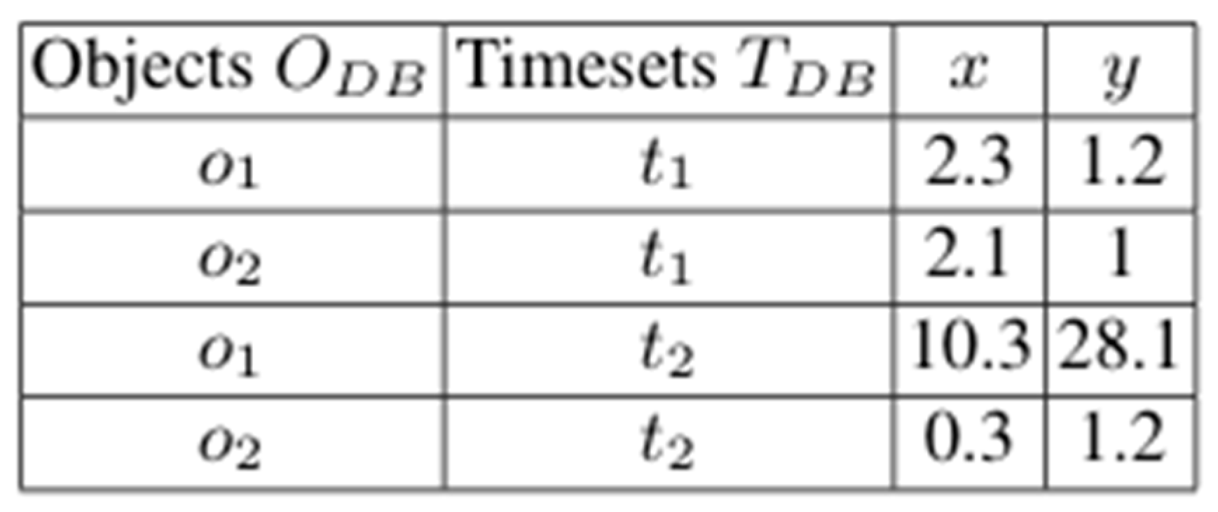
Figure 2.
Representation of spatial temporal data as a space-time cube [30]. The temporal aspect of the data is maintained as separate layers on top of a 2D embedding space. The time series analysis comes from analyzing the vertical column at a position, whereas the temporal layer focuses on the x-y plane as lateral slices.
Figure 2.
Representation of spatial temporal data as a space-time cube [30]. The temporal aspect of the data is maintained as separate layers on top of a 2D embedding space. The time series analysis comes from analyzing the vertical column at a position, whereas the temporal layer focuses on the x-y plane as lateral slices.
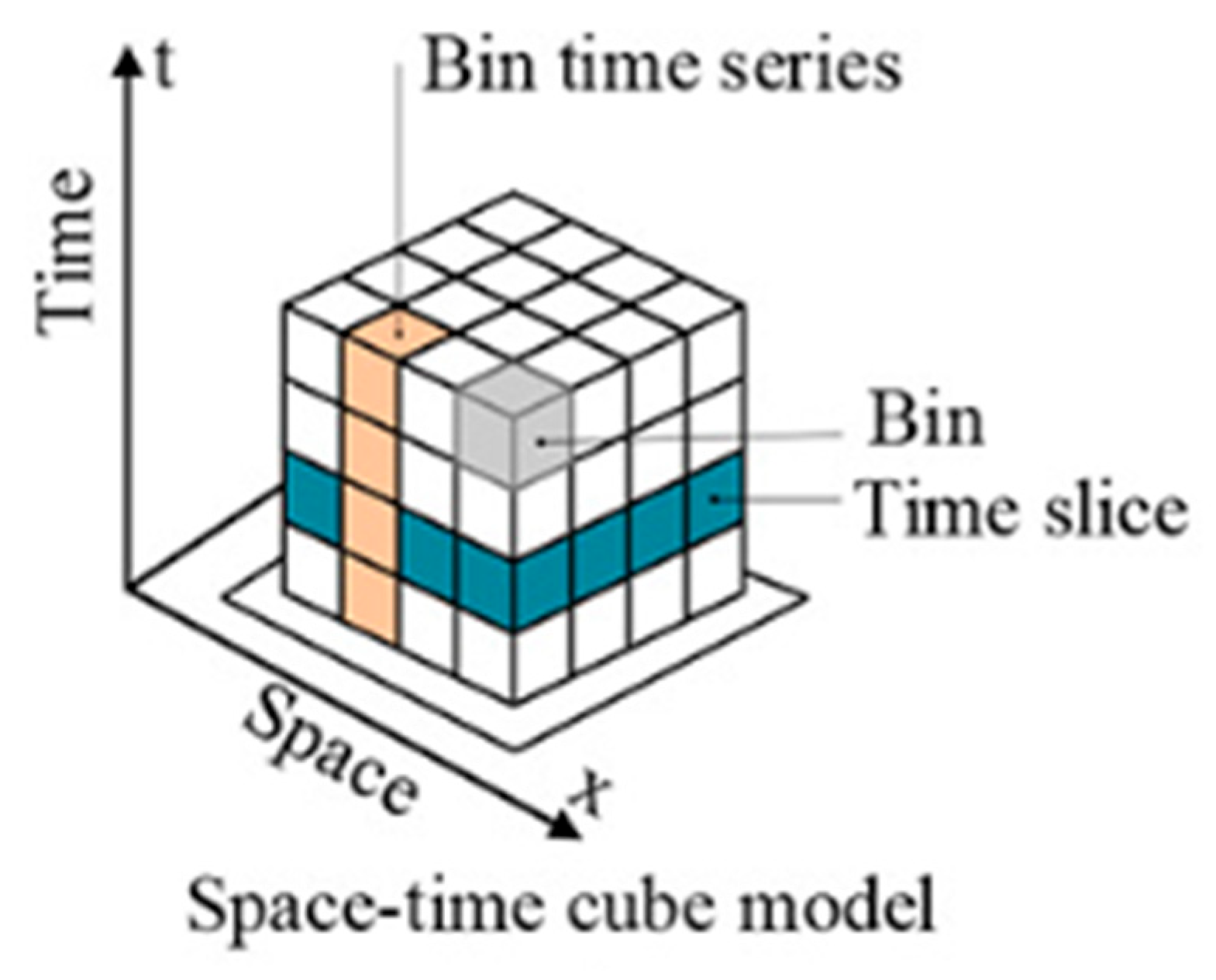
Figure 3.
General workflow for processing spatiotemporal raster data using Spacetime. Unprocessed raster files are imported as Spacetime file objects using read_data() and spatially aligned and cropped using raster_align(). The processed files are converted into multidimensional space-time cubes using make_cube(), enabling temporal scaling, mathematical operations, and other transformations. Modified cubes can subsequently be exported as new file objects and written to disk for further analysis.
Figure 3.
General workflow for processing spatiotemporal raster data using Spacetime. Unprocessed raster files are imported as Spacetime file objects using read_data() and spatially aligned and cropped using raster_align(). The processed files are converted into multidimensional space-time cubes using make_cube(), enabling temporal scaling, mathematical operations, and other transformations. Modified cubes can subsequently be exported as new file objects and written to disk for further analysis.
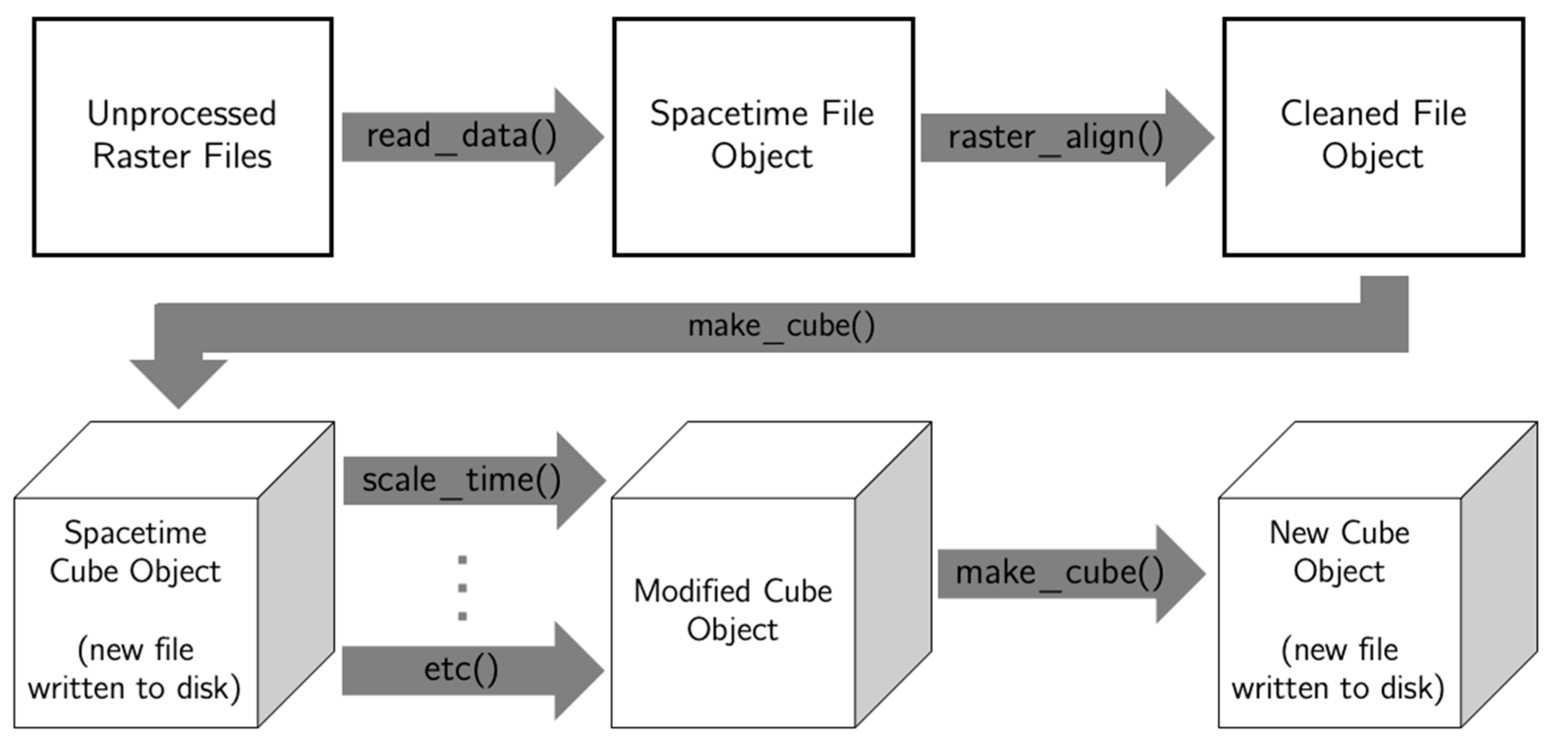
Figure 4.
Workflow for generating future daily temperature projections using the delta method. Schematic illustrating the integration of daily maximum-temperature observations from Daymet (2019) with projected monthly climatologies from CHELSA (2020–2040, SSP5-8.5). Historical daily rasters were spatially aligned with the CHELSA dataset and aggregated into monthly means. Monthly temperature anomalies were calculated by subtracting historical monthly means from projected monthly climatologies, expanded to daily resolution, and added to the corresponding historical daily observations. The resulting dataset preserves the daily weather sequence of 2019 while adjusting temperatures to reflect projected future climatological conditions.
Figure 4.
Workflow for generating future daily temperature projections using the delta method. Schematic illustrating the integration of daily maximum-temperature observations from Daymet (2019) with projected monthly climatologies from CHELSA (2020–2040, SSP5-8.5). Historical daily rasters were spatially aligned with the CHELSA dataset and aggregated into monthly means. Monthly temperature anomalies were calculated by subtracting historical monthly means from projected monthly climatologies, expanded to daily resolution, and added to the corresponding historical daily observations. The resulting dataset preserves the daily weather sequence of 2019 while adjusting temperatures to reflect projected future climatological conditions.
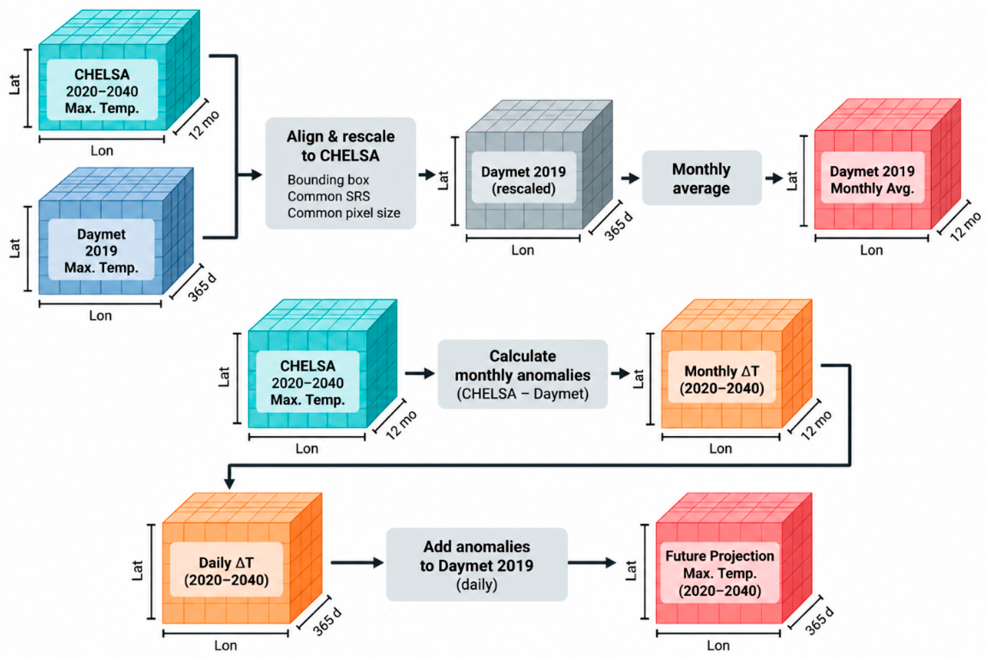
Figure 5.
Computational runtime across spatial resolutions and resampling methods. Execution time (seconds, logarithmic scale) for GDAL and Spacetime across the same pixel-size sequences and resampling methods used in 2.2. Resolution sweeps were conducted using bases of 1, 5, and the native raster resolution to evaluate computational scaling and identify artifacts associated with particular pixel sizes.
Figure 5.
Computational runtime across spatial resolutions and resampling methods. Execution time (seconds, logarithmic scale) for GDAL and Spacetime across the same pixel-size sequences and resampling methods used in 2.2. Resolution sweeps were conducted using bases of 1, 5, and the native raster resolution to evaluate computational scaling and identify artifacts associated with particular pixel sizes.
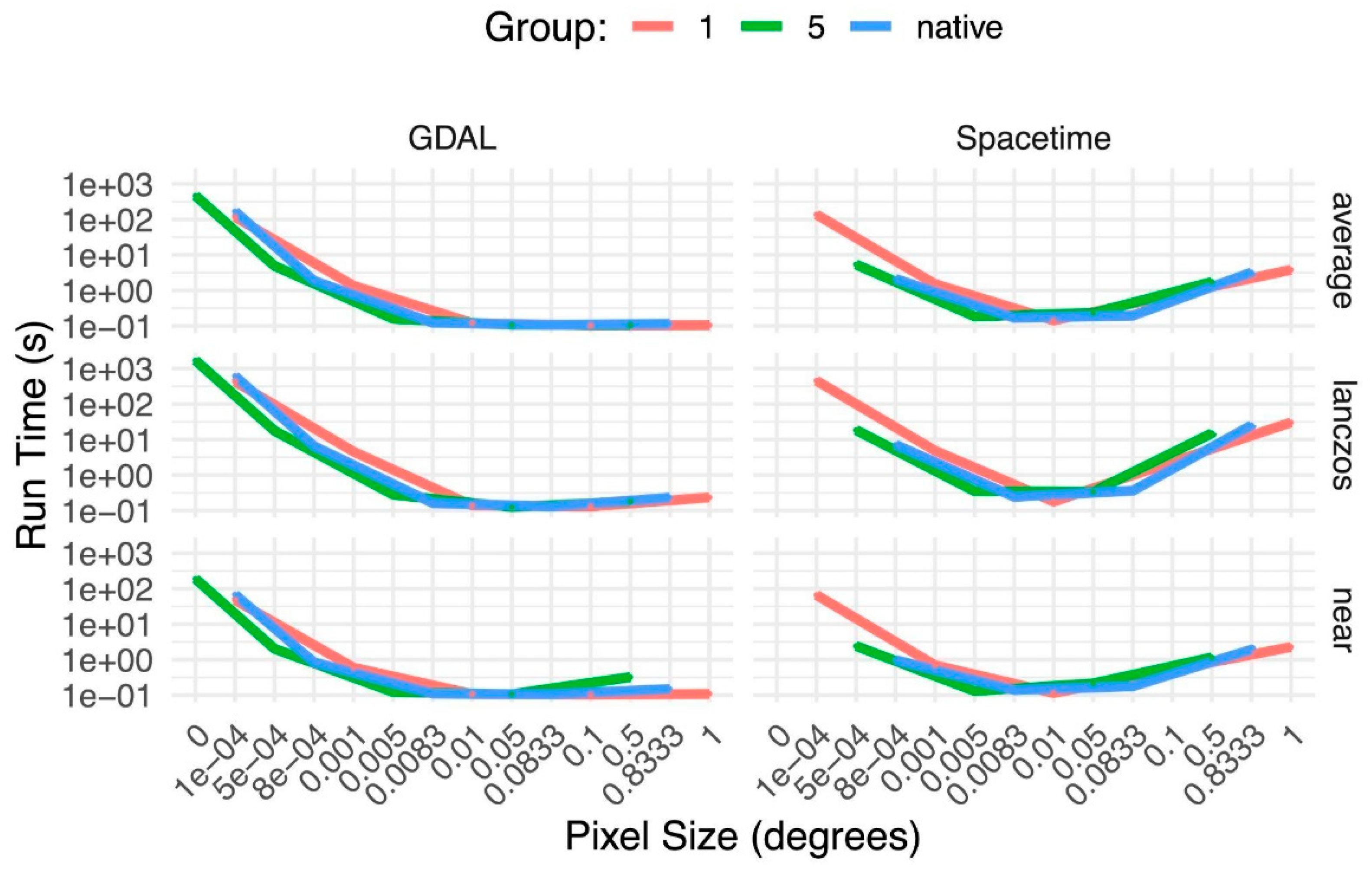
Figure 6.
Computational performance and code complexity of the delta-method case study. Mean execution time (bars) for GDAL, Rasterio, and Spacetime across 30 independent runs of the same spatiotemporal processing workflow explained in Section 2.2. Error bars represent 1 standard error. Diamonds indicate the number of lines of code required to complete the workflow, plotted on the secondary axis.
Figure 6.
Computational performance and code complexity of the delta-method case study. Mean execution time (bars) for GDAL, Rasterio, and Spacetime across 30 independent runs of the same spatiotemporal processing workflow explained in Section 2.2. Error bars represent 1 standard error. Diamonds indicate the number of lines of code required to complete the workflow, plotted on the secondary axis.
Disclaimer/Publisher’s Note: The statements, opinions and data contained in all publications are solely those of the individual author(s) and contributor(s) and not of MDPI and/or the editor(s). MDPI and/or the editor(s) disclaim responsibility for any injury to people or property resulting from any ideas, methods, instructions or products referred to in the content. |
© 2026 by the authors. Licensee MDPI, Basel, Switzerland. This article is an open access article distributed under the terms and conditions of the Creative Commons Attribution (CC BY) license (http://creativecommons.org/licenses/by/4.0/).
Copyright: This open access article is published under a Creative Commons CC BY 4.0 license, which permit the free download, distribution, and reuse, provided that the author and preprint are cited in any reuse.