
Submitted:
02 November 2026
Posted:
03 November 2026
You are already at the latest version
Abstract
Campus heat recovery depends on the coincidence of computing output, thermal demand and required delivery temperature. This study develops an hourly energy–exergy model with bounded storage, boiler backup and an explicit investment threshold expressed as recovered-source utilisation. A synthetic annual campus profile is evaluated at 45, 55 and 70 °C, with three storage capacities and 100 computing-load realisations. Without storage, raising delivery temperature from 45 to 70 °C increases the supplied heat share from 83.1% to 87.2%, yet reduces recovered-source utilisation from 60.6% to 52.5% because compressor electricity contributes more heat. Corresponding net present values are £333,374 and −£347,066 under stated assumptions. At 55 °C, adding 2.4 MWh storage raises supplied heat from 1,696.2 to 1,817.5 MWh but changes investment value from £57,349 to −£13,933. An equal-demand calendar counterfactual changes the direction of the schedule effect as storage increases. The results distinguish thermal feasibility, operating savings and capital recovery, providing conditional screening thresholds rather than validated campus forecasts.
Keywords:
data-centre heat recovery
; exergy analysis
; academic calendars
; thermal storage
; investment thresholds
1. Introduction
University computing facilities produce heat while teaching buildings require it intermittently. Their physical proximity creates an attractive recovery opportunity, but annual energy totals cannot establish whether heat is available at a useful temperature and time. Reviews identify temperature quality and conversion requirements as persistent constraints on data-centre heat reuse [1,2,3]. Experimental evidence is already substantial: Aquasar demonstrated hot-water cooling with direct energy reuse [4], while subsequent field and laboratory studies examined heat-pump-assisted recovery and integrated cooling systems [5,6]. The engineering question concerns usable heat under specified operating conditions.
Lower distribution temperatures can improve access to otherwise underused thermal resources. Fourth-generation district heating integrates lower-temperature supply with wider energy-system operation [7], and European fifth-generation networks demonstrate approaches using near-ambient loops [8]. Large heat pumps provide a practical connection between such resources and conventional heating networks [9]. Nevertheless, performance depends on temperature lift, refrigerant and cycle configuration [10]; detailed campus-oriented heat-pump comparisons confirm that architecture matters [11]. A screening model should therefore expose its temperature assumptions without presenting a simplified coefficient of performance as a manufacturer-validated operating map.
Heat availability also depends on the receiving system. London modelling established the relevance of matching data centres with neighbouring heating requirements [12]. District-heating simulations subsequently connected load profiles and heat procurement prices to recovery performance [13], while commercial coordination emerged as a broader implementation issue [14]. Viewing a data centre as an energy prosumer further connects computing, cooling and downstream heat use [15]. Investment analysis already accommodates uncertainty and price sensitivity [16]. These findings caution against treating a technical recovery percentage as sufficient evidence of financial attractiveness.
Integrated assessment itself is established. Luo and colleagues combined source–sink compatibility, exergy, temporal availability, costs and environmental effects within decision support [17]. More recent work investigates recovery mismatch [18] and hourly energy–exergy performance with heat pumps and seasonal storage [19]. Consequently, another integrated framework is insufficient as a research contribution. A more precise opportunity is to make the investment boundary auditable: identify how much recoverable source heat must actually be used, distinguish that quantity from compressor-enhanced delivered heat, and separate the value of recovery from the incremental value of storage.
Universities make this distinction consequential because academic schedules modify occupancy and thermal demand. Calendar effects have been quantified [20], and campus demand estimates depend on occupancy-model choice [21]. Practical deployment is also established: Queen Mary University of London reports recovering computing heat for its Priestley Building and Mile End network [22]. That institutional announcement supplies context, not operating measurements for this study. Dvorak and colleagues already examined university data-centre recovery, aquifer storage and uncertainty using campus evidence [23]. The present analysis therefore makes no claim to be the first dynamic campus heat-recovery assessment.
Storage must be evaluated against the duration of the mismatch it addresses. Norwegian campus analysis distinguishes short-term tanks from borehole storage [24]; ETH Zurich research considers daily and seasonal interactions [25], and recent campus optimisation jointly sizes seasonal heating and cooling storage [26]. These studies motivate a deliberately narrower test of short-duration buffering. Established demand-overlap measures already quantify temporal complementarity [27]. Here, a calendar counterfactual preserves annual demand while changing its chronology, allowing schedule effects to be distinguished from differences in total heat consumption.
This study develops a reproducible hourly experiment coupling a recovered-heat interface, a heat pump, bounded thermal storage and boiler backup. It derives a conditional source-utilisation threshold and evaluates temperature–storage interactions against gas and ambient-source heat-pump benchmarks. Particular attention is paid to three decisions often conflated in feasibility screening: whether the heat can reach the required temperature, whether operation saves variable expenditure, and whether those savings repay the installed equipment over its assumed remaining economic life. Its contribution is an inspectable decision test, rather than a universal optimum: additional recovered heat may coexist with lower net present value. Synthetic inputs and conditional uncertainty are reported explicitly, establishing the limits within which the numerical conclusions can support subsequent campus measurements and engineering design.
2. Methodology
An hourly, 365-day synthetic experiment represents a campus heat-recovery subsystem. No campus telemetry, measured weather or equipment calibration is used. The boundary begins at recoverable heat at 35 °C and ends at an idealised campus delivery interface (Figure 1). Computing electricity is invariant and excluded from incremental costs and emissions. Distribution losses, cooling-electricity credits, embodied impacts and potable-water requirements are outside scope. Table 1 specifies analyst-selected inputs; Appendix A defines every profile. Chronological simulation avoids disconnected representative periods, whose treatment can distort storage operation [28,29,30].
Computing power combines a daily cycle with stationary autoregressive noise. Heating demand couples a sinusoidal outdoor temperature with weekday occupancy and 240 synthetic term days. A counterfactual removes term closures and rescales the entire resulting demand series to the original annual total. Nine reference designs combine three delivery temperatures with three storage capacities. One hundred independently seeded computing trajectories repeat every design; their fifth–ninety-fifth percentiles describe conditional numerical variability, not confidence intervals or population risk. Additional sweeps vary computing scale and delivery temperature.
Equations (1)–(3) enforce heat-pump and storage energy balances. Absolute temperatures are in kelvin; thermal rates are in kilowatts and the time step is one hour. The heat-pump surrogate includes approach temperatures and a capacity limit. Unaided direct delivery fails the prescribed pinch constraint; preheating a colder return is outside this model. Dispatch first serves demand, then charges available storage, then discharges against residual demand; unused source heat is rejected and a boiler supplies the remainder. Heat-pump operation is screened against the variable cost of boiler heat. This causal heuristic is not predictive economic optimisation; campus dispatch research illustrates more sophisticated alternatives [31].
Equation (4) measures recovery-only exergy under isothermal source and delivery reservoir approximations, with a fixed 288.15 K reference. It does not resolve refrigerant states, water-return temperatures or tank stratification. Equations (5)–(7) calculate discounted investment value, operational emissions and conditional source-utilisation thresholds. Annual costs repeat in real terms for twenty years, with no escalation, salvage or replacement expenditure. Such simplifications differ from stochastic storage planning [32] and lifetime network optimisation [33,34]. Installed-capacity costs and emission factors are scenario assumptions, not quotations or current national statistics. Repeating each annual trajectory to periodic storage convergence prevents free initial energy. Conservation, capacity and nonnegative exergy-destruction checks are complemented by half-hour dispatch using unchanged hourly inputs; these are numerical verification, not physical validation.
All inputs are assumptions for a synthetic screening experiment, not fitted campus values, market quotations or national emission factors. K = K₀ + 30 Emax. Existing boiler capital is sunk; boiler replacement and fixed maintenance are excluded. The ambient-source benchmark omits defrost and part-load effects.
2.1. Coupled Model Equations
Rates a, c and d denote direct delivery, charging and discharging. Unsuffixed H, D and G are annual sums. All energy sums use Δt. M is operational emissions. Equation (7) is prospective without storage; with storage, y and e depend on realised dispatch. Appendix A supplies implementation details.
3. Numerical Results and Discussion
The reference simulation produces 1,999.7 MWh of annual demand and 2,365.7 MWh of recoverable computing heat. Annual source availability therefore exceeds demand, yet considerable source heat remains unused. Figure 2 exposes the chronological constraint, while Table 2 reports all nine designs. At delivery temperatures of 45, 55 and 70 °C, modelled heat-pump coefficients of performance are 7.271, 4.997 and 3.482. These are consequences of the specified surrogate, not measured seasonal performance. The source-to-delivery difference must also accommodate two 5 K approaches.
Without storage, delivered heat rises from 1,661.1 MWh at 45 °C to 1,743.0 MWh at 70 °C. Judged by demand coverage alone, the higher-temperature design appears better: 87.2% rather than 83.1%. However, source utilisation falls from 60.6% to 52.5%, and incremental electricity increases from 245.1 to 518.1 MWh. The additional compressor contribution explains the apparent improvement. Heat delivered divided by available source heat is consequently unsuitable as a recovery fraction. Source extraction and purchased electricity must remain separate ledger entries.
Reference seed 2026; source use = extracted recovered heat / available captured heat. Electricity includes compressor and circulation. Each recovery design uses gas backup to serve the same 1,999.7 MWh annual demand. NPV is relative to continued operation of existing gas heating.
The no-storage investment thresholds in Figure 3 are 32.0%, 49.7% and 710.4% source utilisation at 45, 55 and 70 °C, respectively. The last exceeds the physical maximum, excluding capital recovery under these assumptions even if all available source heat were used. Nevertheless, its direct operating margin remains slightly positive, approximately £0.00128 per delivered kilowatt-hour before fixed maintenance. Physical feasibility, positive variable savings and positive investment value are therefore distinct tests. Reference net present values are £333,374, £57,349 and −£347,066, respectively.
Figure 3 shows curve uses annual available source heat of 2.366 GWh, £300,000 investment, annual maintenance of 2% of capital, electricity at £0.22/kWh, gas at £0.06/kWh fuel, 90% boiler efficiency, and a 20-year horizon discounted at 5%. A point above the curve yields positive NPV under these assumptions. Required utilization exceeds 100% above approximately 63.4 °C; the curve is truncated beyond the physical utilization range. The curve is a conditional investment identity, not a universal technology limit.
Storage improves heat supply without consistently improving investment value (Figure 4). At 55 °C, 0.6 MWh adds 67.9 MWh of annual heat delivery but reduces net present value by £9,351. Increasing storage to 2.4 MWh adds 121.3 MWh relative to no storage while reducing value by £71,282, making the project negative. At 45 °C, the smaller store produces a modest £1,737 incremental gain; the larger store loses £55,015. These capacities represent only 1.5 and 6 hours at rated charging power.
Calendar effects are conditional rather than universally adverse. At equal annual demand, replacing term closures with year-round weekday teaching reduces 55 °C no-storage delivery from 1,696.2 to 1,680.1 MWh and net present value from £57,349 to £53,258. With 2.4 MWh storage, the same counterfactual increases delivery from 1,817.5 to 1,838.6 MWh and improves value from −£13,933 to −£9,344. Rescaling changes load concentration, which interacts with capacity and storage. This sign reversal qualifies any simple assumption that removing holiday shutdowns necessarily improves recovery.
Across 100 computing-load realisations, the 55 °C no-storage net present value has a median of £57,699 and a fifth–ninety-fifth percentile range of £56,774–£58,535. The corresponding 2.4 MWh design remains negative throughout that interval, from −£14,419 to −£11,852. Paired incremental value for the 45 °C, 0.6 MWh store has a median of £1,794 and a range of £1,004–£2,730. These narrow ranges reflect stochastic workload variation around a fixed mean; they omit uncertain tariffs, capital costs, weather, degradation and behavioural responses.
Markers and connecting lines show the synthetic reference year (seed 2026); vertical whiskers show the conditional 5th–95th percentiles across 100 computing-load realizations, with all other assumptions fixed. These intervals describe simulated workload variability and are not confidence intervals for measured performance. Many whiskers are narrower than the marker size. NPV includes storage cost of £30/kWh, maintenance at 2% of total capital, and the same tariffs and discounting as Figure 3. The heat axis is intentionally narrowed because points encode values rather than bar lengths.
Financial sensitivity is larger than workload uncertainty. At the realised no-storage heat output, the electricity tariff compatible with zero net present value is £0.3292/kWh at 45 °C, £0.2329/kWh at 55 °C and £0.1662/kWh at 70 °C. The 55 °C case therefore has limited headroom above the assumed £0.22/kWh. Likewise, the 45 °C, 0.6 MWh store breaks even at an installed storage cost of £32.32/kWh, only modestly above the assumed £30/kWh. These thresholds support prioritising verified quotations and operating tariffs before refining stochastic workload forecasts; apparent numerical precision should not imply investment certainty.
Exergy and carbon provide complementary assessments. No-storage subsystem exergy destruction increases from 181.4 to 319.3 MWh of exergy between 45 and 70 °C. Its exergy efficiency nevertheless changes only from 46.3% to 46.7%, because the useful heat also has higher thermodynamic quality. At the assumed emission factors, annual emissions fall from 406.6 tonnes for gas heating to 133.0 tonnes for 55 °C recovery without storage. The idealised ambient-source comparator emits 159.7 tonnes but has higher discounted heat cost (Table 3).
Numerical closure is satisfactory: energy residuals remain below 0.000001 kWh, and halving the dispatch step changes annual delivered heat by less than 0.017 MWh and investment value by less than £6. These checks establish implementation consistency, not agreement with equipment measurements. Moreover, the energy-priority controller can charge storage uneconomically at 70 °C because cycling losses exceed its narrow variable margin. Predictive control could avoid such charging. The broader conclusion is conditional: storage warrants incremental appraisal, and neither annual heat abundance nor increased heat coverage alone establishes a sound investment. Their transferability remains contingent on site-specific engineering.
All systems meet identical demand. Heat cost includes annualised new capital, electricity, residual gas and fixed maintenance, where applicable. Common campus services and existing boiler capital are excluded. The ambient-source heat pump is a simplified full-demand benchmark, not a calibrated equipment comparison.
4. Conclusions
A chronological energy–exergy screening model shows that campus heat recovery requires separate tests of thermal feasibility, operating margin and capital recovery. Under the stated synthetic assumptions, increasing delivery temperature raises the proportion of demand supplied while reducing the proportion of computing heat actually recovered. This divergence results from additional compressor electricity and demonstrates why heat coverage cannot substitute for source utilisation. The derived break-even identity makes the investment requirement explicit and identifies cases where the required utilisation exceeds physical availability.
Short-duration storage increases supplied heat but often reduces net present value. At 55 °C, the 2.4 MWh store changes an otherwise positive investment into a negative one. An equal-demand calendar comparison also reverses the direction of the schedule effect as storage increases, showing that academic closures interact with load concentration and capacity constraints.
These conclusions are conditional on assumed costs, fixed-temperature reservoirs and heuristic dispatch. Future validation should combine metered computing power, source and return temperatures, campus demand, equipment performance maps and installed-cost evidence. Testing predictive control and tariff uncertainty would establish whether the small storage benefit survives realistic operating conditions and whether the screening thresholds transfer to a specific estate.
Supplementary Materials
The following supporting information can be downloaded at the website of this paper posted on Preprints.org.
Data Availability Statement
All results are deterministic profile recipe and seeded simulation described in Appendix A. The accompanying computational archive contains the complete model, parameter record, scenario outputs, paired simulation ensemble and editable figure sources. No confidential or measured university dataset is used.
Appendix A. Reproducible Specification
A.1. Profiles and Numerical Sequence
Let t run from 0 to 8,759, d = floor(t/24), and h = t mod 24. Day 0 is Monday in a synthetic non-leap year. Term days are d ∈ [0,85), [105,175) and [265,350). Occupancy o is 1 on term weekdays between 08:00 and 18:00, 0.15 at other term hours, and 0.05 during vacations. The continuous 80 kW base load represents generic useful thermal demand; it is not a potable-hot-water assumption.
NumPy default_rng with its PCG64 generator uses reference seed 2026 and ensemble seeds 0–99. The initial normal draw is followed by 8,759 innovation draws. Every seed is paired across all designs. Computing-scale checks multiply the clipped profile by 0.6, 0.8, 1.0, 1.2 or 1.4. The temperature sweep covers 45–70 °C at 1 °C intervals. Monthly aggregates use standard non-leap-year month lengths, independent of the synthetic term definition. All rates are held constant within each hourly step.
The equal-demand calendar comparison uses year-round weekday occupancy of 1 from 08:00 to 18:00 and 0.15 otherwise, then multiplies the resulting total demand series by 0.9505704628. This preserves annual demand while changing its distribution. The half-hour check repeats each hourly rate twice and uses λ½ = 1 − (1 − 0.001)^0.5. It verifies the dispatch discretisation without introducing new subhourly weather or demand information.
A.2. Dispatch and Thermodynamic Accounting
Before Equation (2), set Qmax,t to zero if cg/ηb − ce(1/κ + α) ≤ 0. This screen does not bind in the reference designs. Apply standing loss before charging. The available charging volume and discharge inventory in Equation (2) enforce state bounds; surplus and deficit do not coexist, preventing simultaneous charging and discharging. Repeat the same annual trajectory until the initial and final store states differ by less than 10⁻⁹ kWh. Store losses comprise λEt, (1 − ηc)ctΔt and (1/ηd − 1)dtΔt. Initial and final energy are included in the numerical conservation check.
Equation (4) assigns heat exergy to constant-temperature source and delivery reservoirs. Pump electricity and storage losses dissipate to the reference environment. Under periodic storage, no net exergy is carried between years. This calculation does not substitute for finite-stream exergy, which would require measured supply, return and mass-flow values. For an incompressible stream, the rate of thermal exergy change is ṁcp[(Tout − Tin) − T₀ ln(Tout/Tin)]. Component temperatures and stratification are not inferred from the lumped reservoir representation.
A.3. Threshold Interpretation and Benchmark
For no storage, y = 1/(1 − 1/κ) and e = (1/κ + α)/(1 − 1/κ), so Equation (7) gives a prospective threshold at fixed temperature and annual source availability. A threshold above one cannot be attained; if m ≤ 0, no positive source utilisation recovers capital. With storage, y and e include realised losses and dispatch, making the threshold conditional. Differentiating NPV with respect to utilisation holds those factors fixed. The threshold is an accounting boundary, not an independent prediction of achievable utilisation.
Holding dispatch fixed, the electricity tariff at zero NPV is ce* = [Hcg/ηb − F − K/A]/W. For incremental storage, let ΔR be the annual saving in fuel and electricity before additional maintenance. Its break-even installed price per unit capacity is kstore* = AΔR/[Emax(1 + 0.02A)]. Negative values mean that the heuristic increases variable costs even before storage capital is charged. The ambient-source benchmark substitutes Ta,t for Ts in the heat-pump surrogate, supplies all demand, and uses a capacity of 777.5 kW with capital of £505,375. Common boiler capital remains excluded.
References
- Ebrahimi, K.; Jones, G. F.; Fleischer, A. S. A review of data center cooling technology, operating conditions and the corresponding low-grade waste heat recovery opportunities. Renew. Sustain. Energy Rev. 2014, vol. 31, 622–638. [Google Scholar] [CrossRef]
- Yuan, X.; Liang, Y.; Hu, X.; Xu, Y.; Chen, Y.; Kosonen, R. Waste heat recoveries in data centers: A review. Renew. Sustain. Energy Rev. 2023, vol. 188, Art. no. 113777. [Google Scholar] [CrossRef]
- Hao, Y.; et al. Data centers waste heat recovery technologies: Review and evaluation. Appl. Energy 2025, vol. 384, Art.(no. 125489). [Google Scholar] [CrossRef]
- Zimmermann, S.; Meijer, I.; Tiwari, M. K.; Paredes, S.; Michel, B.; Poulikakos, D. Aquasar: A hot water cooled data center with direct energy reuse. Energy 2012, vol. 43(no. 1), 237–245. [Google Scholar] [CrossRef]
- He, Z.; Ding, T.; Liu, Y.; Li, Z. Analysis of a district heating system using waste heat in a distributed cooling data center. Appl. Therm. Eng. 2018, vol. 141, 1131–1140. [Google Scholar] [CrossRef]
- Chen, X.; Wang, X.; Ding, T.; Li, Z. Experimental research and energy saving analysis of an integrated data center cooling and waste heat recovery system. Appl. Energy 2023, vol. 352, Art. no. 121875. [Google Scholar] [CrossRef]
- Lund, H.; et al. Generation District Heating (4GDH): Integrating smart thermal grids into future sustainable energy systems. Energy 2014, vol. 68, 1–11. [Google Scholar] [CrossRef]
- Buffa, S.; Cozzini, M.; D’Antoni, M.; Baratieri, M.; Fedrizzi, R. 5th generation district heating and cooling systems: A review of existing cases in Europe. Renew. Sustain. Energy Rev. 2019, vol. 104, 504–522. [Google Scholar] [CrossRef]
- David; Mathiesen, B. V.; Averfalk, H.; Werner, S.; Lund, H. Heat Roadmap Europe: Large-Scale Electric Heat Pumps in District Heating Systems. Energies 2017, vol. 10(no. 4), Art. no. 578. [Google Scholar] [CrossRef]
- Arpagaus; Bless, F.; Uhlmann, M.; Schiffmann, J.; Bertsch, S. S. High temperature heat pumps: Market overview, state of the art, research status, refrigerants, and application potentials. Energy 2018, vol. 152, 985–1010. [Google Scholar] [CrossRef]
- Wang, P.; et al. District heating utilizing waste heat of a data center: High-temperature heat pumps. Energy Build. 2024, vol. 315, Art.(no. 114327). [Google Scholar] [CrossRef]
- Davies, G. F.; Maidment, G. G.; Tozer, R. M. Using data centres for combined heating and cooling: An investigation for London. Appl. Therm. Eng. 2016, vol. 94, 296–304. [Google Scholar] [CrossRef]
- Wahlroos, M.; Pärssinen, M.; Manner, J.; Syri, S. Utilizing data center waste heat in district heating – Impacts on energy efficiency and prospects for low-temperature district heating networks. Energy 2017, vol. 140, 1228–1238. [Google Scholar] [CrossRef]
- Wahlroos, M.; Pärssinen, M.; Rinne, S.; Syri, S.; Manner, J. Future views on waste heat utilization – Case of data centers in Northern Europe. Renew. Sustain. Energy Rev. 2018, vol. 82, 1749–1764. [Google Scholar] [CrossRef]
- Huang, P.; et al. A review of data centers as prosumers in district energy systems: Renewable energy integration and waste heat reuse for district heating. Appl. Energy 2020, vol. 258, Art. no. 114109. [Google Scholar] [CrossRef]
- Pärssinen, M.; Wahlroos, M.; Manner, J.; Syri, S. Waste heat from data centers: An investment analysis. Sustain. Cities Soc. 2019, vol. 44, 428–444. [Google Scholar] [CrossRef]
- Luo, Y.; Andresen, J.; Clarke, H.; Rajendra, M.; Maroto-Valer, M. A decision support system for waste heat recovery and energy efficiency improvement in data centres. Appl. Energy 2019, vol. 250, 1217–1224. [Google Scholar] [CrossRef]
- Wang, J.; Guo, Y.; Yue, C.; Deng, W.; Zeng, L. Comprehensive assessment of waste heat recovery mismatch and renewable energy integration in data centers: A multifaceted energy, economic, and environmental perspectives. J. Clean. Prod. 2024, vol. 472, Art. no. 143466. [Google Scholar] [CrossRef]
- Verzino; Talluri, L.; Rocchetti, A.; Socci, L. Smart Reuse of Waste Heat from Data Centres: Energy and Exergy Analysis for a District-Heating Network in Bulgaria. Energies 2026, vol. 19(no. 3, Art. no. 800). [Google Scholar] [CrossRef]
- Gui, X.; Gou, Z.; Lu, Y. Reducing university energy use beyond energy retrofitting: The academic calendar impacts. Energy Build. 2021, vol. 231, Art. no. 110647. [Google Scholar] [CrossRef]
- Al-Saegh, S.; Kourgiozou, V.; Korolija, I.; Tang, R.; Tahmasebi, F.; Mumovic, D. Investigating building stock energy and occupancy modelling approaches for district-level heating and cooling energy demands estimation in a university campus. Energy Build. 2025, vol. 329, Art.(no. 115269). [Google Scholar] [CrossRef]
- Queen Mary University of London, “Queen Mary University of London data centre waste heat to provide hot water and heating for campus,” Dec. 9, 2024. Available online: https://www.qmul.ac.uk/news/latest-news/2024/se/queen-mary-university-of-london-data-centre-waste-heat-to-provide-hot-water-and-heating-for-campus.html (accessed on Nov. 2 2026).
- Dvorak, V.; Zavrel, V.; Torrens Galdiz, J. I.; Hensen, J. L. M. Simulation-based assessment of data center waste heat utilization using aquifer thermal energy storage of a university campus. Build. Simul. 2020, vol. 13(no. 4), 823–836. [Google Scholar] [CrossRef]
- Li, H.; Hou, J.; Hong, T.; Ding, Y.; Nord, N. Energy, economic, and environmental analysis of integration of thermal energy storage into district heating systems using waste heat from data centres. Energy 2021, vol. 219, Art. no. 119582. [Google Scholar] [CrossRef]
- Gabrielli, P.; Acquilino, A.; Siri, S.; Bracco, S.; Sansavini, G.; Mazzotti, M. Optimization of low-carbon multi-energy systems with seasonal geothermal energy storage: The Anergy Grid of ETH Zurich. Energy Convers. Manag. X 2020, vol. 8, Art.(no. 100052). [Google Scholar] [CrossRef]
- Zhang, R.; Li, Z.; Liu, P. Modeling and optimization of a heating and cooling combined seasonal thermal energy storage system towards a carbon-neutral community: A university campus case study. Energy 2025, vol. 319, Art.(no. 135122). [Google Scholar] [CrossRef]
- Wirtz, M.; Kivilip, L.; Remmen, P.; Müller, D. Quantifying Demand Balancing in Bidirectional Low Temperature Networks. Energy Build. 2020, vol. 224, Art. no. 110245. [Google Scholar] [CrossRef]
- Kotzur, L.; Markewitz, P.; Robinius, M.; Stolten, D. Time series aggregation for energy system design: Modeling seasonal storage. Appl. Energy 2018, vol. 213, 123–135. [Google Scholar] [CrossRef]
- van der Heijde, B.; Vandermeulen, A.; Salenbien, R.; Helsen, L. Representative days selection for district energy system optimisation: a solar district heating system with seasonal storage. Appl. Energy 2019, vol. 248, 79–94. [Google Scholar] [CrossRef]
- Blanke, T.; Schmidt, K. S.; Göttsche, J.; Döring, B.; Frisch, J.; van Treeck, C. Time series aggregation for energy system design: review and extension of modelling seasonal storages. Energy Inform. 2022, vol. 5, Art.(no. 17). [Google Scholar] [CrossRef]
- Campos, G.; et al. Optimal real-time dispatching of chillers and thermal storage tank in a university campus central plant. Appl. Energy 2021, vol. 300, Art. no. 117389. [Google Scholar] [CrossRef]
- Egging-Bratseth, R.; Kauko, H.; Knudsen, B. R.; Bakke, S. A.; Ettayebi, A.; Haufe, I. R. Seasonal storage and demand side management in district heating systems with demand uncertainty. Appl. Energy 2021, vol. 285, Art. no. 116392. [Google Scholar] [CrossRef]
- Wirtz, M.; Kivilip, L.; Remmen, P.; Müller, D. 5th Generation District Heating: A novel design approach based on mathematical optimization. Appl. Energy 2020, vol. 260, Art. no. 114158. [Google Scholar] [CrossRef]
- Wirtz, M.; Heleno, M.; Romberg, H.; Schreiber, T.; Müller, D. Multi-period design optimization for a 5th generation district heating and cooling network. Energy Build. 2023, vol. 284, Art.(no. 112858). [Google Scholar] [CrossRef]
Figure 1.
System boundary for the numerical heat-recovery study. Recovered source heat at 35 °C is upgraded and delivered directly or through thermal storage. Electricity covers compressor and circulation demand; auxiliary electricity is not credited as useful heat. The gas boiler supplies the residual campus load. Unchanged IT electricity, possible cooling-energy savings and distribution-network losses are excluded. Arrows indicate energy pathways, not scaled flow magnitudes; the store does not charge and discharge simultaneously.
Figure 1.
System boundary for the numerical heat-recovery study. Recovered source heat at 35 °C is upgraded and delivered directly or through thermal storage. Electricity covers compressor and circulation demand; auxiliary electricity is not credited as useful heat. The gas boiler supplies the residual campus load. Unchanged IT electricity, possible cooling-energy savings and distribution-network losses are excluded. Arrows indicate energy pathways, not scaled flow magnitudes; the store does not charge and discharge simultaneously.
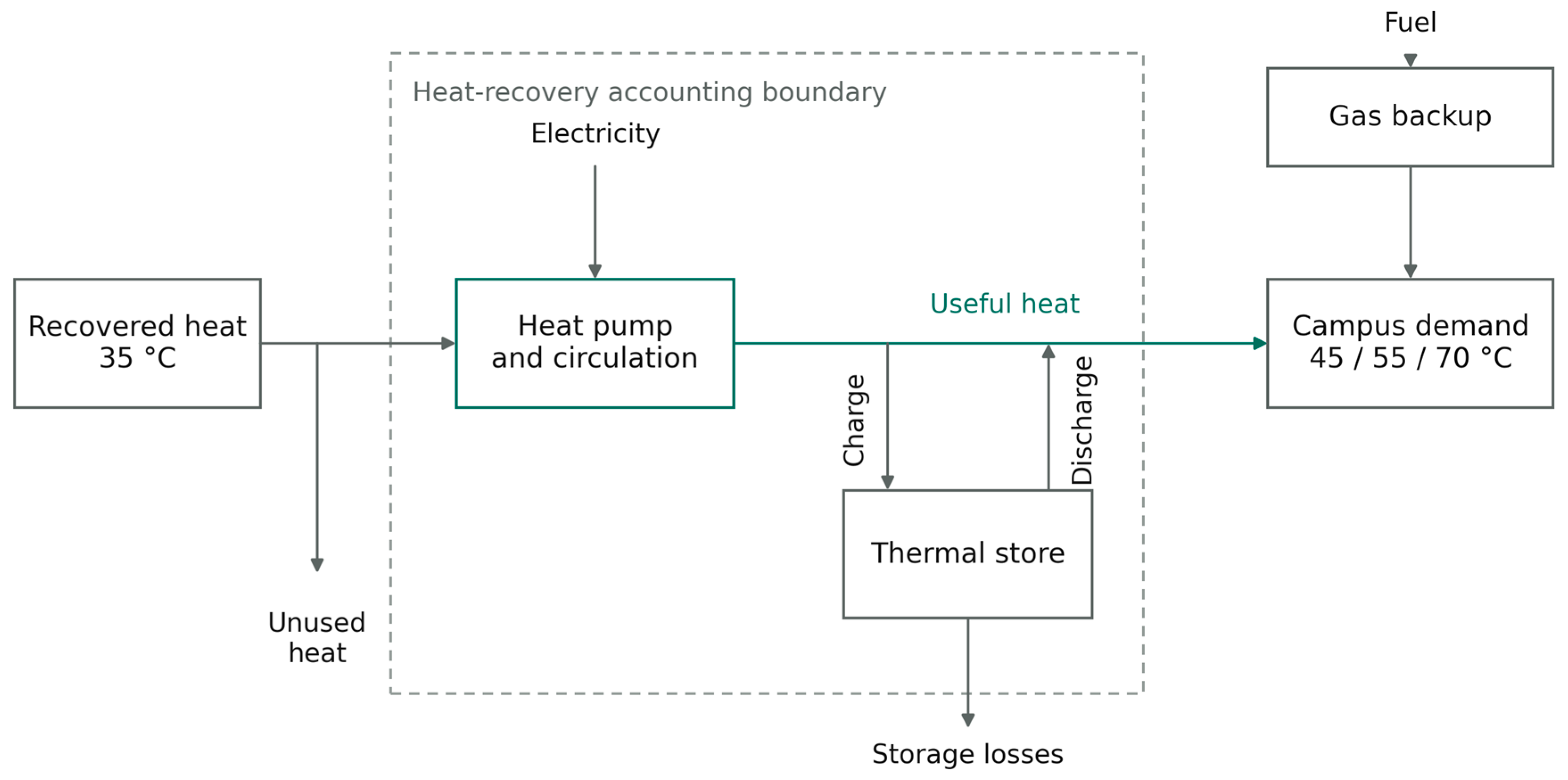
Figure 2.
Monthly energy balances for the synthetic reference year (seed 2026), 55 °C delivery and 0.6 MWh storage: (a) available and used recovered source heat; (b) campus heat demand and heat delivered by recovery. The source-side and delivery-side quantities are separated because compressor electricity increases heat-pump output. Monthly sums use a non-leap-year calendar; annual demand is approximately 2.000 GWh. These are simulated values, not measured university data.
Figure 2.
Monthly energy balances for the synthetic reference year (seed 2026), 55 °C delivery and 0.6 MWh storage: (a) available and used recovered source heat; (b) campus heat demand and heat delivered by recovery. The source-side and delivery-side quantities are separated because compressor electricity increases heat-pump output. Monthly sums use a non-leap-year calendar; annual demand is approximately 2.000 GWh. These are simulated values, not measured university data.
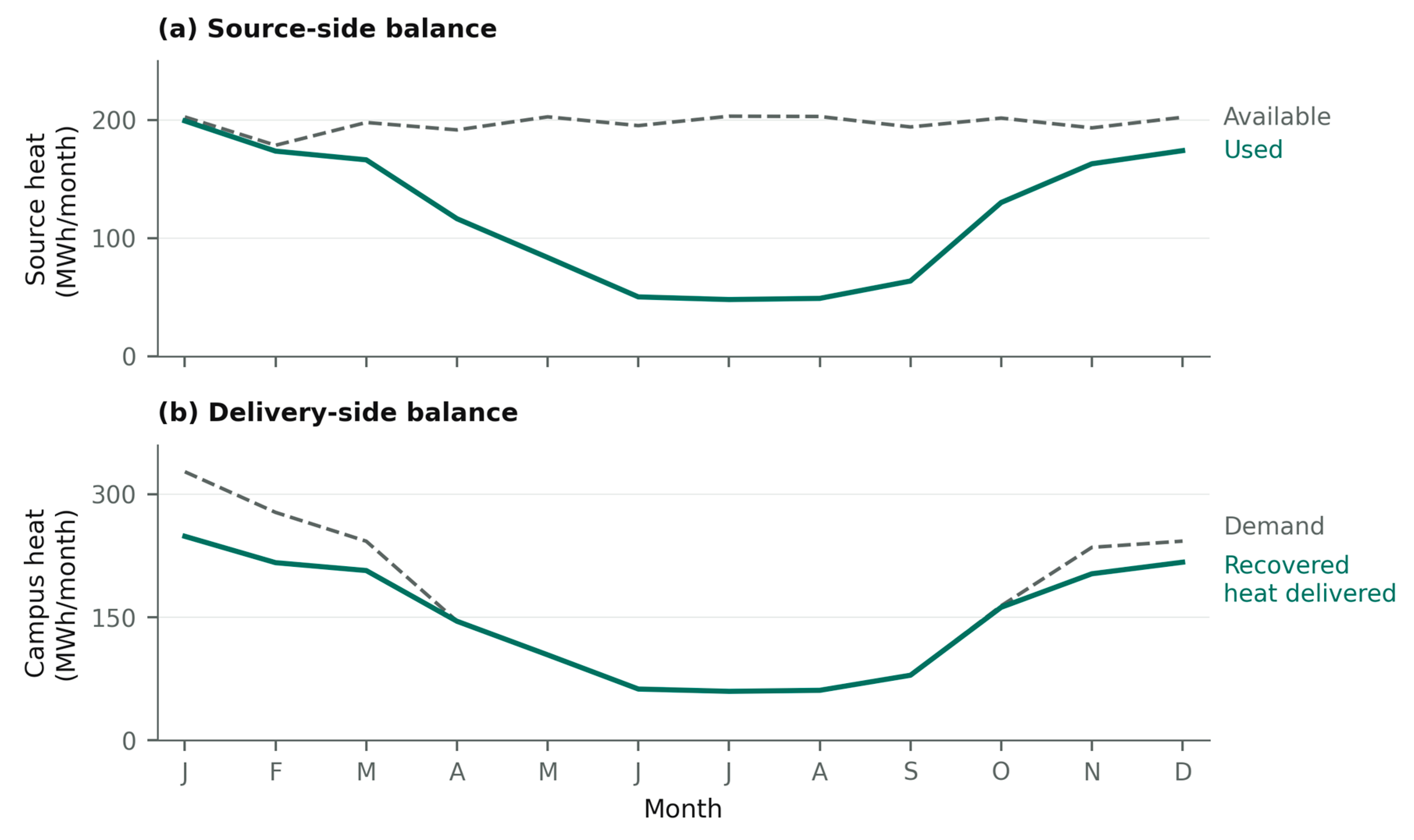
Figure 3.
Analytical no-storage break-even recovered-source utilization against delivery temperature, with the simulated seed-2026 operating points at 45, 55 and 70 °C.
Figure 3.
Analytical no-storage break-even recovered-source utilization against delivery temperature, with the simulated seed-2026 operating points at 45, 55 and 70 °C.
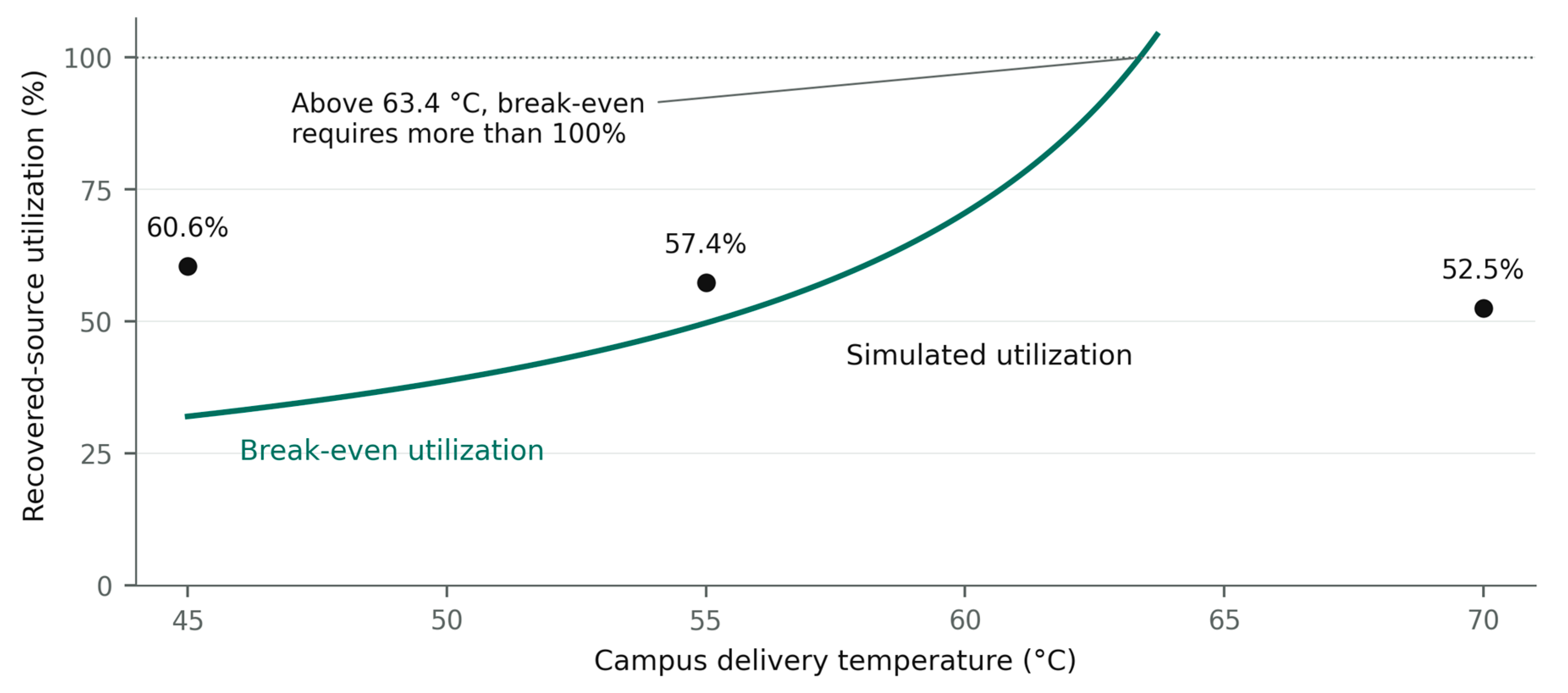
Figure 4.
Storage capacity changes (a) annual recovered heat delivered and (b) heat-recovery project NPV at three delivery temperatures.
Figure 4.
Storage capacity changes (a) annual recovered heat delivered and (b) heat-recovery project NPV at three delivery temperatures.
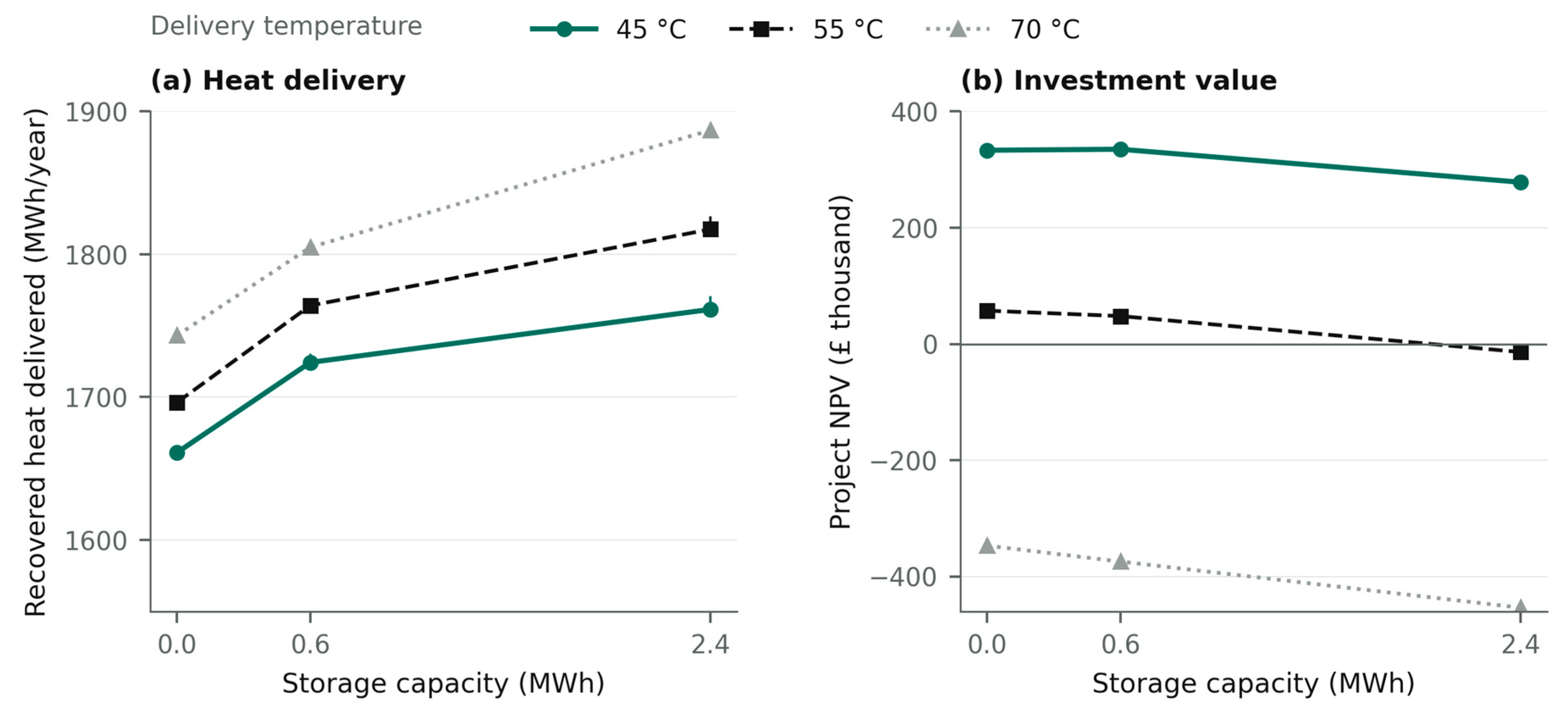

Table 1.
Analyst-selected inputs for the numerical experiment.
| Parameter | Value or definition | Basis |
| Recoverable heat temperature Tₛ | 35 °C | Isothermal source |
| Delivery temperature Tₕ | 45 / 55 / 70 °C | Three separate designs |
| Heat capture fraction ηcap | 0.90 | Fraction of computing power |
| Heat-pump limit Qcap / relative Carnot efficiency | 400 kW / 0.45 | Constant surrogate |
| Approach δ / COP ceiling | 5 K at each side / 8 | Temperature constraint |
| Pump fraction α | 0.01 | Electricity per heat-pump output |
| Storage capacity Emax / power limit | 0 / 600 / 2,400 kWh; 400 kW | Hot-side energy buffer |
| Charge and discharge efficiencies | ηc = ηd = 0.98 | Each direction |
| Hourly storage loss λ | 0.001 | Fraction of initial state |
| Boiler efficiency ηb | 0.90 | Fuel-to-heat efficiency |
| Electricity ce / gas cg | £0.22 / £0.06 per kWh | Electricity / fuel basis |
| Recovery capital K₀ / storage unit cost | £300,000 / £30 per kWh | Installed-cost scenarios |
| Fixed maintenance F / project horizon | 0.02 K per year / 20 years | Repeated real annual costs |
| Real discount r / exergy reference T₀ | 5% / 288.15 K | Fixed reference conditions |
| Emission factors fe / fg | 0.20 / 0.183 kg CO₂e per kWh | Electricity / fuel scenarios |
| Ambient-source benchmark capital | £650 per kW; 777.5 kW | Peak-load capacity |
Table 2.
Annual simulated recovery outcomes and discounted investment value.
|
Delivery (°C) |
Store (MWh) |
Heat H (MWh) |
Source use (%) |
Electricity (MWh) |
NPV (£1,000) |
| 45 | 0.0 | 1,661.1 | 60.6 | 245.1 | 333.4 |
| 45 | 0.6 | 1,724.3 | 63.1 | 255.4 | 335.1 |
| 45 | 2.4 | 1,761.4 | 64.9 | 262.7 | 278.4 |
| 55 | 0.0 | 1,696.2 | 57.4 | 356.4 | 57.3 |
| 55 | 0.6 | 1,764.1 | 59.9 | 372.2 | 48.0 |
| 55 | 2.4 | 1,817.5 | 62.2 | 386.3 | -13.9 |
| 70 | 0.0 | 1,743.0 | 52.5 | 518.1 | -347.1 |
| 70 | 0.6 | 1,805.0 | 54.6 | 538.6 | -374.4 |
| 70 | 2.4 | 1,886.9 | 57.6 | 567.8 | -453.9 |
Table 3.
Whole-system heat cost and operational emissions against alternative heat supplies.
| Heat supply |
Delivery (°C) |
Electricity (MWh/year) |
Heat cost (£/kWh) |
Emissions (t CO₂e/year) |
| Existing gas boiler | All | 0.0 | 0.0667 | 406.6 |
| Recovery + gas, no store | 45 | 245.1 | 0.0533 | 117.9 |
| Recovery + gas, no store | 55 | 356.4 | 0.0644 | 133.0 |
| Recovery + gas, no store | 70 | 518.1 | 0.0806 | 155.8 |
| Ambient-source heat pump | 45 | 684.8 | 0.1007 | 137.0 |
| Ambient-source heat pump | 55 | 798.3 | 0.1132 | 159.7 |
| Ambient-source heat pump | 70 | 956.2 | 0.1305 | 191.2 |
Disclaimer/Publisher’s Note: The statements, opinions and data contained in all publications are solely those of the individual author(s) and contributor(s) and not of MDPI and/or the editor(s). MDPI and/or the editor(s) disclaim responsibility for any injury to people or property resulting from any ideas, methods, instructions or products referred to in the content. |
© 2026 by the authors. Licensee MDPI, Basel, Switzerland. This article is an open access article distributed under the terms and conditions of the Creative Commons Attribution (CC BY) license (http://creativecommons.org/licenses/by/4.0/).
Copyright: This open access article is published under a Creative Commons CC BY 4.0 license, which permit the free download, distribution, and reuse, provided that the author and preprint are cited in any reuse.