

Submitted:
31 October 2026
Posted:
03 November 2026
You are already at the latest version
Abstract
Conventional reservoir-level measurement systems convert hydrostatic pressure into an electrical signal, which makes the entire sensing chain dependent on electronic components that are vulnerable to lightning-induced transients, power interruption, and long-term environmental degradation. This paper proposes a hydromechanical measurement architecture in which hydrostatic pressure is converted directly into an n-bit digital code through a purely mechanical successive-approximation procedure, with no electrical component anywhere in the sensing or comparison chain. A lever-balance comparator, pivoting on a knife-edge, is weighed against a reference column fed by a bank of individually calibrated, laminar-flow binary-pressure orifices; a fixed manual protocol, structurally identical to the classical single-pan binary-weight problem, halves the search interval at each of n steps, resolving the most significant bit first. A Monte Carlo simulation propagating a physically-derived, bit-dependent orifice calibration-retention error, differential fluid-density mismatch, and comparator friction through the full binary-search procedure identifies a practical operating point of n = 10 bits, giving an effective resolution of approximately 1.4 mm (7.7 effective bits) over a 1.024 m bench-scale range. The architecture extends our prior demonstration that the successive-approximation principle is independent of the specific physical quantity involved, showing here that it is also independent of the electrical domain altogether.
Keywords:
hydrostatic pressure
; hydromechanical sensing
; binary search
; successive approximation
; laminar hydraulic orifice calibration
; electronics-free measurement
; reservoir level
1. Introduction
The decomposition of an unknown quantity into a weighted sum of binary-valued decisions predates electronic instrumentation by several centuries. As early as 1202, Fibonacci posed the problem of determining an unknown integer weight using the fewest reference weights on a single-pan balance; Bachet de Méziriac later gave the systematic solution for this case — weights in powers of two — showing that any integer up to 2ⁿ − 1 can be resolved in exactly n comparisons [1,2,3]. This is, in essence, the same successive-approximation principle later re-implemented electronically in the successive-approximation-register (SAR) analogue-to-digital converter [4], where binary-weighted reference voltages replace physical weights and an electronic comparator replaces the balance beam.
We have previously shown that this principle is not tied to any single electrical quantity: a companion study replaces the capacitive reference network of a conventional SAR ADC with a binary-weighted resistive network for multi-sensor telemetry [5], following an initial study that established significance-weighted (nonuniform) physical tolerance allocation for binary-weighted measurement systems [6]. The present work asks a different question. Rather than substituting one electrical component for another, it asks whether the comparison itself — the mechanism that decides a binary digit b_i ∈ {0,1} — can be removed from the electrical domain entirely. We show that a purely mechanical lever balance, driven by calibrated hydraulic reference volumes, reproduces the same binary-search behaviour without any electrical component in the sensing chain, down to and including fully manual operation.
This is evaluated as a bench-scale proof of principle (full-scale range H_max = 1.024 m) rather than a field-deployable dam instrument; extending the physical scale to tens of metres is identified in Section 6 as a direction for future work, not a claim made here.
1.1. Electronic Reservoir-Level Measurement
Conventional hydrostatic level measurement submerges a pressure transducer at a fixed depth and reports a continuous electrical signal proportional to head [7,8,16]. Recent reviews of dam- and reservoir instrumentation confirm that essentially all deployed monitoring architectures, from submersible piezometers to distributed fibre-optic pressure sensing, ultimately terminate in an electronic acquisition stage [9,10]. Pneumatic bubbler systems avoid submerging electronics by relaying pressure through an air column [11], but still terminate in an electrical pressure cell for readout — the electrical dependency is relocated within the system, not removed from it. Even recent low-cost and passive-wireless sensing efforts, which specifically target harsh-environment robustness, retain an electronic transduction or telemetry stage at some point in the chain [12,13,14,15]; the electronics-free comparison mechanism proposed here is, to our knowledge, a different point in this design space rather than a competing solution to the same deployment constraints.
1.2. Successive Approximation as a General, Substrate-Independent Principle
The mathematical core of the SAR ADC — repeatedly halving an uncertainty interval using binary-weighted references — is identical to the classical balance-weighing problem discussed above [1,2,3]. Standard treatments of SAR conversion emphasize that the settling time of each comparison, not the comparison principle itself, sets the fundamental speed/accuracy trade-off of the architecture [4]; this observation applies without modification to a hydraulic or mechanical embodiment of the same principle, as developed in Section 2 and Section 5 below.
1.3. Author's Prior Work
Our first study in this line of work developed significance-weighted (nonuniform) tolerance allocation for binary-weighted measurement systems, giving a closed-form allocation rule together with its validity boundary [6]. A second, companion study replaced the capacitive reference network with a binary-weighted resistive network for ADC-less, multi-sensor telemetry [5], establishing that the successive-approximation principle transfers between electrical quantities. The present paper takes a further, qualitatively distinct step relative to [5]: rather than substituting one electrical reference quantity for another, it removes the electrical substrate from the comparison mechanism altogether, replacing it with a mechanical lever balance and calibrated hydraulic pressure thresholds (Section 2 and Section 3). The technical content, error model, and simulation results reported below are entirely new to this domain and share no derivation or text with or [6].
2. Proposed Measurement Principle
2.1. Principle
The hydrostatic pressure at a measurement point located at depth h below the free surface of the reservoir is, for a fluid of density ρ, given by
where P_atm is atmospheric pressure and g is gravitational acceleration. For the gauge pressure P_g = ρ g h, the water head follows directly as
P = P_atm + ρ g h
h = P_g / (ρ g)
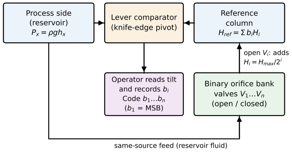
Rather than measuring P_g continuously, the architecture proposed here compares it sequentially against a set of n calibrated pressure thresholds, producing one binary decision per comparison. The physical realisation consists of three elements and one procedure:
(i) a lever comparator pivoting on a hardened knife-edge (Section 2.3);
(ii) a bank of n binary-pressure orifices, each fitted with an independent, manually operated two-state (open/closed) valve (Section 2.2 and Section 3);
(iii) a manual binary-search protocol executed by an operator (Section 2.4).
Figure 1.
System architecture: the process side and a common reference column are compared by a lever balance; opening valve V_i admits a calibrated pressure increment H_i into the reference column, and the resulting decisions form the binary output code.
Figure 1.
System architecture: the process side and a common reference column are compared by a lever balance; opening valve V_i admits a calibrated pressure increment H_i into the reference column, and the resulting decisions form the binary output code.
2.2. Hydraulic Binary Threshold Bank
For an n-bit code and a full-scale range H_max, the target pressure threshold associated with bit i (i = 1 … n, with i = 1 the most significant bit) is
ΔP_i = ρ g (H_max / 2ⁱ)
Each threshold is realised by one binary-pressure orifice (Section 3) controlled by a dedicated, manually operated valve V_i. Every valve has exactly two states — fully open or fully closed — which is what makes the decision at each step genuinely binary rather than a continuous adjustment; no orifice is ever partially opened during a measurement.
2.3. Manual Comparator
The comparator is a lever balance pivoting on a hardened knife-edge, with the process-side diaphragm and the reference-side diaphragm at equal arm lengths, each of area A_m. Mechanical equilibrium requires
and the operator reads the direction of tilt — process side down, reference side down, or level — with a simple pointer or spirit-level indicator. No electrical signal is generated or required at any point in this comparison.
F_x = P_x A_m , F_ref = P_ref A_m
A key design choice is that the reference-column fluid is drawn from the same source as the process fluid (the reservoir itself, or a representative sample of it), rather than being a fixed laboratory fluid. Writing the equilibrium condition explicitly in terms of density,
if ρ_x = ρ_ref because both are drawn from the same source, density and gravitational acceleration cancel completely, leaving h_x = H_ref: the system becomes a pure head comparator. This eliminates the common-mode density error entirely (temperature, atmospheric pressure); only the differential density mismatch between the local measurement point and the reference sample — for example from localised sedimentation or salinity — remains, and is retained explicitly as σ_density in Section 5.
ρ_x g h_x = ρ_ref g H_ref
2.4. Manual Binary-Search Procedure
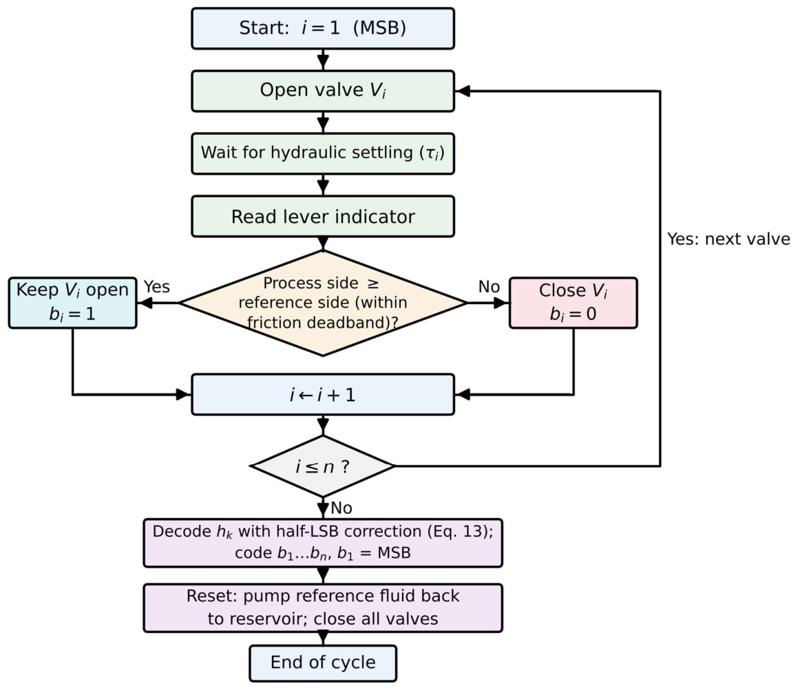
The operator follows a fixed, written protocol — a standard operating procedure, not a judgment call — identical in structure to the successive-approximation logic used in electronic SAR ADCs [4], but executed entirely by hand, for i = 1 to n (i.e. starting from the most significant bit and proceeding towards the least significant, consistent with valve V_1 being the largest-threshold, most significant valve of Figure 3):
1. Open valve V_i.
2. Wait for hydraulic settling, characterised by the time constant τ_i = R_h,i C_h,i of the orifice-column combination.
3. Read the lever indicator.
4. If the process side remains at or above the reference side (within the friction deadband of Section 5), leave V_i open and record bit b_i = 1.
5. Otherwise, close V_i and record bit b_i = 0.
6. Proceed to valve V_{i+1} and repeat from step 1.
After V_n, the recorded bits b_1 … b_n (b_1 the most significant) form the digital code. This procedure is structurally identical to the Fibonacci/Bachet single-pan weighing solution of Section 1 — at each step, a candidate binary weight (here, a hydraulic pressure threshold) is tentatively added, and kept only if the balance does not tip the wrong way. We note that resolving the most significant bit first, rather than the least significant, is essential to the correctness of the search: only once the largest threshold has been decided does halving the remaining interval at each subsequent step correctly bound the unknown value, exactly as in the classical binary-weighing problem of Section 1.
Before the apparatus is ready for a subsequent measurement, two further steps restore it to its initial state (Section 6): the reference-column fluid is pumped back to the reservoir through the return line — a manual pump for the bench-scale prototype described here, an electric pump for a field-deployed version — and all n valves are closed. Only after this reset is the procedure of steps 1–6 repeated for the next measurement.
Figure 2.
Manual binary-search procedure. Each of the n iterations opens one valve, allows hydraulic settling, and records one bit according to the comparator reading. After the code is decoded, the reference-column fluid is pumped back to the reservoir and all valves are closed before the next measurement cycle begins (Section 6).
Figure 2.
Manual binary-search procedure. Each of the n iterations opens one valve, allows hydraulic settling, and records one bit according to the comparator reading. After the code is decoded, the reference-column fluid is pumped back to the reservoir and all valves are closed before the next measurement cycle begins (Section 6).
3. Detailed Experimental Setup Specification
3.1. Physical Realization of the Orifice Bank
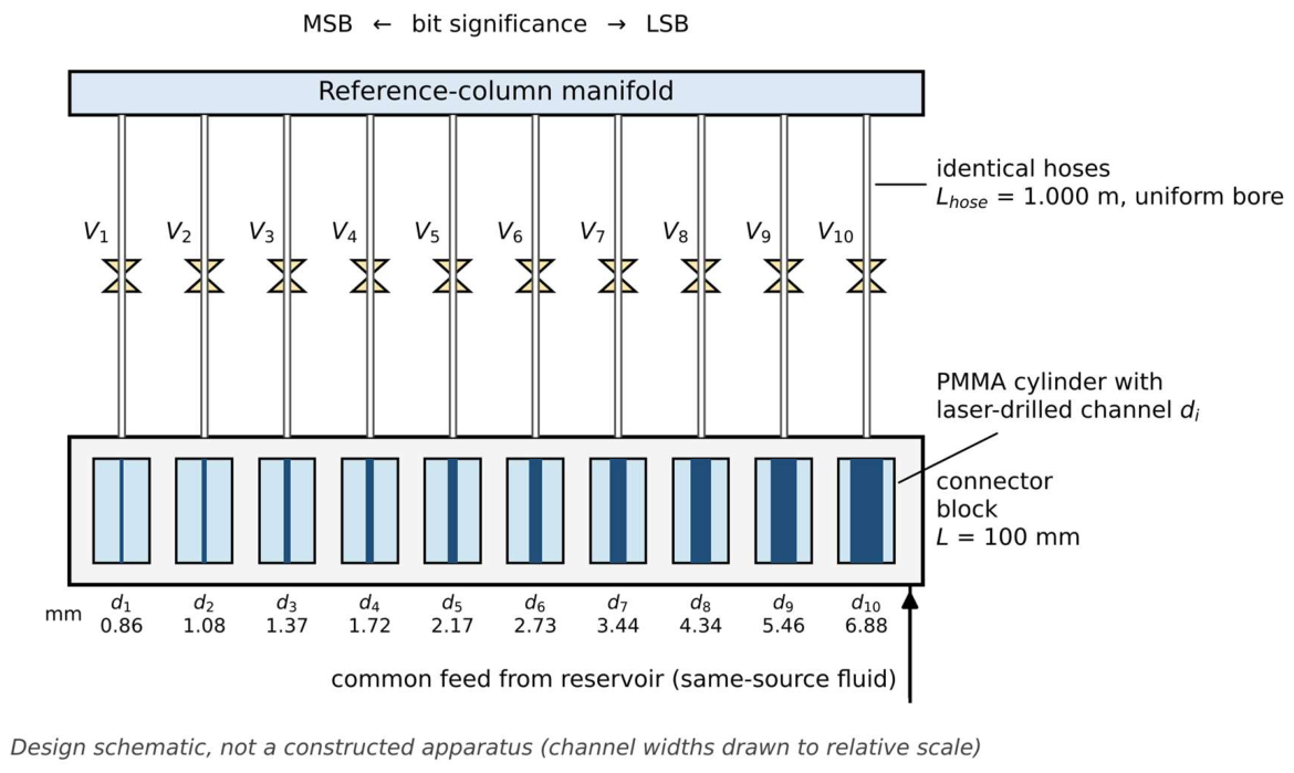
Rather than realizing the n individually calibrated pressure thresholds of Eq. (3) through orifices of differing cross-section machined into distinct hose fittings, the present design uses hydraulically identical hoses (inner bore uniform, length L_hose = 1.000 m for every channel) connecting the reference-column manifold to a single connector block. The connector block contains n precision-bored seats, each housing a cylinder whose central channel is produced by a single-pass laser drilling operation; plexiglass (PMMA) is adopted here for the water-based bench prototype for its transparency, ease of laser machining, and low cost, but the cylinder material is a design choice rather than a requirement of the architecture — a design engineer is free to substitute any material offering easier manufacturability or higher mechanical strength (e.g., for higher-pressure ranges or oil-based field deployments), subject to re-characterizing its dimensional stability as in Section 3.4. It is this laser-drilled channel — not the hose — that realizes the calibrated hydraulic resistance R_h,i for bit i. This separation of functions (hose = transport, cylinder = calibrated restriction) removes hose-to-hose geometric variability from the error budget entirely: every channel sees the same entrance/exit hose geometry, and only the laser-bored cylinder differs between bits.
Figure 3.
Conceptual schematic of the connector block: n = 10 hydraulically identical 1 m hoses feed a common block containing n precision-bored seats, each housing a laser-drilled plexiglass cylinder that realizes one calibrated binary-pressure threshold (diameters d_1–d_10 from Table 1). Design schematic, not a photograph of a constructed apparatus — no physical prototype has been built at the time of writing.
Figure 3.
Conceptual schematic of the connector block: n = 10 hydraulically identical 1 m hoses feed a common block containing n precision-bored seats, each housing a laser-drilled plexiglass cylinder that realizes one calibrated binary-pressure threshold (diameters d_1–d_10 from Table 1). Design schematic, not a photograph of a constructed apparatus — no physical prototype has been built at the time of writing.
3.2. Fluid Selection
Water is adopted as the working fluid for the bench-scale prototype and for all design equations, error-model figures, and validation numbers reported in this paper (μ = 1.0 mPa·s, ρ = 1000 kg/m³ at room temperature). Water is chosen for practical reasons at this stage of development: it is inexpensive, safe to handle, transparent (permitting the sight-tube readout of Section 3.7), and its properties are well characterized, which keeps the closed-form design of Section 3.4 and the Monte Carlo error model of Section 5 straightforward to validate experimentally.
For an eventual field deployment, the working fluid is expected to be a mineral or synthetic oil rather than water, for two reasons. First, oil is the natural in-situ fluid in several of the target applications identified for this architecture (oil reservoirs, sealed hydraulic systems), removing the need to introduce a foreign fluid into the sensing chain. Second, as discussed in Section 6, an oil-filled, sealed system inherently avoids the biological-fouling failure mode that motivates the water-treatment measures of Section 3.7, since oil does not support microorganism growth.
Switching the working fluid changes μ and ρ in Eqs. (7)–(9), and therefore the specific channel diameters and Reynolds-number margins of Table 1: a more viscous oil, for a fixed Re_target, generally permits larger channel diameters at a given ΔP_i (since d_i scales with μ^(2/3) in Eq. 8), which would further relax the calibration-retention sensitivity discussed in Section 3.4 — a potential secondary benefit of a field-deployed, oil-filled version of this architecture, though one not quantified here. A full re-derivation of Table 1 for a specific candidate oil (viscosity and density depend strongly on oil grade and operating temperature) is identified as a direction for future work, and is not required for the water-based bench-scale validation that is the subject of this paper.
3.3. Governing Flow Regime: From Turbulent Orifice to Laminar Restriction
For an idealised turbulent orifice, the flow rate Q is related to the pressure differential ΔP by
where the discharge coefficient C_d itself depends on the Reynolds number, and this relation was the basis of the original orifice-bank concept. For the plexiglass-cylinder geometry adopted here, however, the channel length-to-diameter ratio places the flow in the laminar regime for every bit of the design (verified in Section 3.5), and the governing relation is instead Hagen–Poiseuille:
where d is the drilled channel diameter, L is the cylinder thickness (equal to the channel length), μ is the dynamic viscosity of the working fluid, and ΔP is the pressure differential across the cylinder. Because Eq. (7) contains two free geometric parameters (d, L) for a single target ΔP_i, the design is closed by fixing L uniformly across all n cylinders and solving for d_i individually (Section 3.4) — analogous in spirit to the trim-to-target calibration philosophy of the original turbulent-orifice concept, but now applied to a laminar rather than turbulent restriction.
Q = C_d A √(2ΔP/ρ)
Q = π d⁴ ΔP / (128 μ L)
3.4. Design Constraint and Closed-Form Solution
L is held fixed across all n cylinders — chosen for ease of manufacture, since a single stock sheet thickness of the chosen cylinder material is laser-cut to seat diameter — and the remaining degree of freedom, d_i, is fixed by requiring a constant target Reynolds number Re_target = 1000 across the full bank, providing a 2.3× safety margin below the laminar-turbulent transition (Re ≈ 2300) for every bit, including the largest-flow channel (LSB). Combining the Reynolds-number definition with Eq. (7) yields the closed-form design equation:
with ΔP_i given by Eq. (3) for a full-scale range H_max = 1.024 m, using water as the working fluid (μ = 1.0 mPa·s, ρ = 1000 kg/m³ at room temperature; see Section 3.2 for the fluid choice and its implications for a future oil-based field version). Table 1 tabulates the design up to n = 12 bits, matching the extended bit depth explored by the error model of Section 5 (Table 3 and Table 4); only the first ten channels are required for the n = 10 practical operating point identified in Section 5, with bits 11–12 included purely for consistency with that analysis.
d_i = [ 32 μ² L Re_target / (ρ ΔP_i) ]^(1/3)
A second consideration beyond Reynolds number bounds the choice of L: because ΔP_i ∝ L/d_i³ (Eq. 7 combined with the Reynolds constraint), any absolute dimensional drift δd of a calibrated channel — from thermal or hygroscopic expansion of the cylinder material, mechanical wear, or biological/particulate fouling — propagates into a relative pressure-threshold error
which is amplified for the narrowest channels. Since ΔP_i is largest for the most significant bit, Eq. (8) makes the MSB channel the narrowest of the bank — precisely the channel whose threshold error is weighted most heavily in the decoded result. Because d_i ∝ L^(1/3) at fixed ΔP_i and Re_target, increasing L raises every channel diameter by a common factor, directly reducing σ_manuf,i for a given δd. We adopt L = 100 mm (a 10 cm-thick connector block, still a compact bench-scale component), which raises the narrowest (MSB) channel from 0.40 mm — the value obtained at L = 10 mm — to 0.86 mm, comfortably inside the range of reliable laser-drilling and manual reaming. Table 1 lists the resulting channel diameters, flow rates, and fill volumes/times for all twelve bits at L = 100 mm.
σ_manuf,i ≈ 3 · δd / d_i
Channels 1–10 realize the n = 10 practical design identified in Section 5; channels 11–12 extend the same closed-form design to n = 12 bits and are shown for direct correspondence with the error-model tables (Table 3 and Table 4) — they are not part of the n = 10 bench-scale design specified in this section. Diameters range from 0.86 mm (bit 1, MSB) to 10.93 mm (bit 12) — the narrowest channel is more than double the L = 10 mm design's MSB channel, substantially reducing sensitivity to dimensional drift at essentially no manufacturing cost (a thicker, not narrower, connector block). As a side benefit, every fill time is shorter than at L = 10 mm because the larger channels pass more flow at the same ΔP_i; bits 11–12 add negligible volume and time to a full measurement (≈ 0.13 mL and ≈ 0.02 s combined), so the total fill time for the practical 10-bit measurement remains ≈ 3.7 min, essentially unchanged whether or not the two extra channels are physically present. Each cylinder is laser-drilled slightly undersized (≈ 0.80 mm for the MSB channel) and brought to its final target diameter by manual reaming, verified against the reference column.
Taking δd ≈ 1 μm as a representative bound on residual dimensional drift — with biological and particulate fouling suppressed by the working-fluid preparation of Section 3.7, the remaining contribution is the hygroscopic/thermal dimensional stability of the cylinder material itself — Eq. (9) gives σ_manuf,1 (MSB) ≈ 0.35% and σ_manuf,10 (LSB) ≈ 0.04%. This bit-dependent σ_manuf,i, rather than a single flat value, is propagated through the Monte Carlo simulation of Section 5. We emphasize two caveats. First, δd = 1 μm is a design assumption consistent with published dimensional-stability figures for machined PMMA — the material adopted here for the water-based bench prototype — not a quantity measured on the specific apparatus described here, since no physical apparatus has been constructed (Section 6); confirming it experimentally remains a prerequisite for any future construction of this design, by the author or by others. Second, since the cylinder material is a design choice rather than a fixed requirement (Section 3.1), an implementing engineer selecting a different material for manufacturability or strength should re-evaluate δd for that material before relying on the σ_manuf,i figures reported here; a stiffer, less hygroscopic material than PMMA would be expected to reduce δd further, tightening the error margins of Table 3 rather than loosening them.
3.5. Reynolds-Number Verification
For a circular channel of diameter d carrying flow rate Q, the Reynolds number is
Re = 4 ρ Q / (π d μ)
Substituting the (d_i, Q_i) pairs of Table 1 confirms Re ≈ 1000 for every channel by construction (Eq. 8 enforces this identically), so all ten channels operate in the laminar regime with a uniform 2.3× margin below transition, independent of bit position.
3.6. Reservoir Sizing for Negligible Level Drop
Two independent constraints bound the reservoir cross-sectional area A_res. First, stability during measurement: the total volume withdrawn during one complete 10-bit measurement (worst case, code 1111111111) is ΣV_i ≈ 181 mL — unchanged from the L = 10 mm design, since V_i = A_ref·H_i depends only on the reference-column geometry and target head increments, not on L. Requiring the resulting level drop to remain below δh_max = 0.25 mm — one LSB at the 12-bit depth of Table 4, and well below the ≈ 1.4 mm effective-resolution floor — sets
corresponding to a cylindrical bench-scale tank of diameter ≈ 96 cm and height slightly exceeding H_max = 1.024 m. Second, manual inlet-valve closure error: setting a target validation level via the graduated sight-tube (Section 3.7) introduces a level error
where δt ≈ 0.3–0.5 s is a representative manual valve-closure reaction time and Q_fill ≈ 0.5–1 L/s is a typical laboratory tap flow rate. With A_res = 0.72 m², δh ≈ 0.04 cm (0.4 mm) — below the system's resolution floor, confirming that the same reservoir sizing satisfies both constraints without requiring a fast-acting or electronically timed inlet valve. We note that the first constraint is a bench-scale validation artifact rather than a fundamental architectural limitation: in field-scale deployments (reservoir, dam, borehole) the reservoir volume is orders of magnitude larger than any volume withdrawn through the orifice bank, and this constraint is automatically satisfied.
A_res ≥ ΣV_i / δh_max ≈ 7240 cm² (≈ 0.72 m²)
δh = Q_fill · δt / A_res
3.7. Manual Reference-Level Setting: Graduated Sight-Tube
To establish a known ground-truth process-side level h_x for validation trials without introducing an additional electrical or optical sensing element, a transparent graduated sight-tube is mounted alongside the reservoir, connected at its base to the reservoir interior. For each target level h_target, the corresponding position is marked on the tube; the operator opens the reservoir's manual inlet valve and closes it when the meniscus reaches the marked line. This uses the same manual, gauge-reading philosophy as the measurement procedure itself (Section 2.4) — the operator reads a physical scale rather than performing a computed comparison — and requires no laser-cut components, solenoids, or timed actuation.
Because the calibration-retention model of Section 3.4 assumes biological and particulate fouling are suppressed, the bench-scale working fluid is prepared accordingly: quadruple-distilled water is used, an inline UV lamp is placed in the water path to suppress microorganism growth, and the reservoir is kept enclosed and dark to prevent photosynthetic growth. Under these measures, the residual dimensional-drift budget of Eq. (9) is attributed to the cylinder material itself rather than to biofouling of the sub-millimetre channels, consistent with the δd ≈ 1 μm assumption of Section 3.4 for the PMMA prototype adopted here.
3.8. Validation Protocol
Following the same statistical-validation philosophy used in a companion binary-weight measurement experiment by the author (N = 40 target masses generated by a seeded pseudorandom generator, to be reported separately), a validation protocol is proposed here on the same basis, for future execution once the apparatus is constructed. A set of N = 40 target levels has been generated in advance as follows: a pseudorandom generator was seeded with the numeric generation date (format YYYYMMDD; the seed value is recorded in the generation script), drawing uniformly from the sub-range 50,970] mm — excluding the extremes of the 0–1024 mm full-scale range, where edge effects (near-empty or near-full reservoir) are not representative of normal operating conditions. Target values were rounded to the nearest 0.5 mm, matching the practical reading resolution of the graduated sight-tube and avoiding false precision relative to the system's own ≈ 1.4 mm resolution floor. Table 2 lists the 40 target levels; the generation script is available from the author (see Data availability) so that whoever constructs the apparatus — the author, should resources permit, or another research group — can reproduce the identical target sequence.

Table 2.
Validation target levels (uniform over [50, 970] mm, rounded to 0.5 mm).
| # | h (mm) | # | h (mm) | # | h (mm) | # | h (mm) |
|---|---|---|---|---|---|---|---|
| 1 | 710.5 | 11 | 311.0 | 21 | 144.0 | 31 | 412.0 |
| 2 | 913.0 | 12 | 86.5 | 22 | 200.0 | 32 | 795.5 |
| 3 | 495.5 | 13 | 306.5 | 23 | 641.0 | 33 | 455.5 |
| 4 | 704.5 | 14 | 191.0 | 24 | 515.0 | 34 | 950.0 |
| 5 | 346.5 | 15 | 328.5 | 25 | 78.5 | 35 | 449.5 |
| 6 | 389.0 | 16 | 722.5 | 26 | 225.5 | 36 | 203.5 |
| 7 | 681.5 | 17 | 488.0 | 27 | 532.0 | 37 | 623.0 |
| 8 | 710.0 | 18 | 66.0 | 28 | 321.0 | 38 | 506.5 |
| 9 | 373.0 | 19 | 567.5 | 29 | 331.5 | 39 | 843.5 |
| 10 | 289.5 | 20 | 598.5 | 30 | 364.5 | 40 | 600.0 |
For each target level, the sight-tube procedure of Section 3.7 would set h_x, after which the manual binary-search procedure (Section 2.4) would be executed and the decoded level h_k (Eq. 13) recorded. Agreement between h_target and h_k across all 40 trials would then be reported via mean absolute error (MAE), root-mean-square error (RMSE), and a decoded-versus-target scatter plot with the y = x reference line — the same reporting format used for the companion mass-measurement validation mentioned above. As no physical apparatus has been constructed at the time of writing (Section 6), this protocol is presented as a fully specified proposal rather than a completed measurement: the target list (Table 2) and its generation script are available, but no raw readings exist yet to accompany them.
4. Worked Example and Reservoir Capacity Conversion
For the bench-scale prototype (H_max = 1.024 m, orifice bank as designed in Section 3), the practical operating point identified through simulation (Section 5) is n = 10 bits. The operator executes the procedure of Section 2.4 ten times, producing a 10-bit code k ∈ {0, …, 1023}. The decoded head, including the half-LSB correction discussed in Section 5, is
giving a nominal resolution of 1 mm before non-ideal effects and an effective resolution of approximately 1.40 mm after them (Table 4, ENOB ≈ 7.7 bits). For a reservoir with a known stage–storage relation V = f(h), stored as a lookup table or as a physical scale on the reference column itself, the measured h_k converts directly to a volume figure without any additional electrical processing — the entire chain from pressure to a human-readable capacity figure can, in principle, be completed without electricity.
h_k = k · (H_max/2^10) + H_max/2^11
5. Error Model and Monte Carlo Simulation
Four physical non-idealities were identified and propagated through a 20,000-trial Monte Carlo simulation of the complete binary-search procedure of Section 2.4 (source code available from the author; see Data availability). Comparator friction/hysteresis is modelled as an equivalent head deadband,
where F_c is the equivalent Coulomb friction force of the knife-edge pivot. Capillary rise in the reference-column tube (bore diameter d) follows Jurin's law,
and, for a 15 mm bore, evaluates to approximately 1.98 mm — a systematic offset that is removed by calibration rather than treated as a random error term. The two remaining sources are orifice calibration retention, modelled as the bit-dependent σ_manuf,i of Eq. (9) with δd = 1 μm (Section 3.4), and differential density mismatch (σ_density, Section 2.3), treated as an independent random variable with relative standard deviation 0.02%, consistent with achievable bench-scale calibration tolerances once common-mode density effects are eliminated by the same-source reference fluid of Eq. (5).
δh_fric = F_c / (A_m ρ g)
h_cap = 4γ cosθ / (ρ g d)
A methodological note on reproducibility: initial simulation runs of the uncorrected decoding rule exhibited a systematic negative bias equal to exactly half the final-bit least-significant-bit (LSB) step — the same round-down effect we previously identified and corrected in a resistive binary-weighing measurement in earlier work. Adding a half-LSB correction term, already reflected in Eq. (13) and in the decoding rule used throughout this section, restored full agreement with the theoretical quantization noise floor for the ideal (non-corrupted) case. A second implementation error was identified and corrected during this simulation work: an earlier draft of the manual procedure (Section 2.4) specified resolving bits from least to most significant, which does not implement a valid binary search; the procedure as stated in Section 2.4 (most significant bit first) is the corrected, verified form.
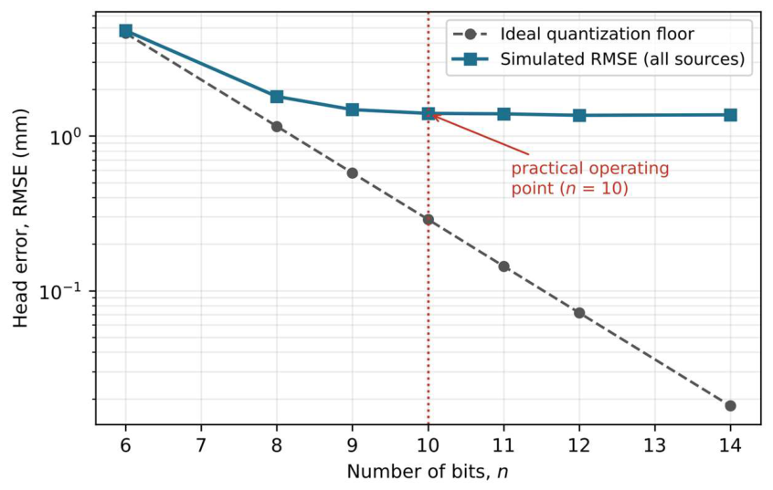
As shown in Table 4 and Figure 4, the simulated RMSE closely tracks the ideal quantization floor through n ≈ 7, then saturates near 1.36–1.40 mm regardless of further bit additions: beyond n ≈ 10, additional orifices increase mechanical complexity without improving accuracy. The sensitivity breakdown of Table 3 confirms that orifice calibration retention dominates by close to an order of magnitude over every other source, identifying it — rather than comparator friction or fluid-density effects — as the limiting factor of this architecture, exactly as in the L = 10 mm design, but now at a level consistent with the physically-derived, bit-dependent σ_manuf,i of Section 3.4 rather than an assumed flat percentage. n = 10 is therefore identified as the practical design point used in Section 4.
Figure 4.
Simulated head-error RMSE versus nominal bit count n, compared against the ideal quantization floor. The curve saturates near n = 10, identifying the practical operating point used throughout this paper.
Figure 4.
Simulated head-error RMSE versus nominal bit count n, compared against the ideal quantization floor. The curve saturates near n = 10, identifying the practical operating point used throughout this paper.
6. Advantages and Practical Limitations
The principal advantage of the proposed architecture is complete independence from electrical components in the sensing chain, giving inherent immunity to lightning-induced transients, power interruption, and electromagnetic interference: the entire measurement, including read-out, can be performed manually with no power source.
This immunity is traded against practical limits that are absent from electronic implementations. First, resolution saturates at approximately 10 effective bits (≈ 1.4 mm over a 1.024 m range) due to orifice calibration retention — a manufacturing limit, not a fundamental one, and one that could in principle be reduced by tighter calibration procedures or a longer connector block (Section 3.4) at modest additional size. Second, each measurement requires n sequential valve operations and settling periods, making the method substantially slower than an electronic ADC and unsuitable for applications requiring rapid or continuous readings. Third, the architecture was evaluated at bench scale (H_max = 1.024 m) using water as the working fluid; extending it to field or dam-scale ranges (tens of metres), re-deriving Table 1 for an oil-based working fluid as outlined in Section 3.2, or re-validating the friction and capillary assumptions of Section 5 for a non-laboratory geometry, are all left as directions for future work.
The biological-fouling mitigation of Section 3.7 (distilled water, inline UV sterilization, reservoir darkness) is specific to the bench-scale validation, where an open, illuminated water reservoir would otherwise support microorganism growth inside the sub-millimetre channels. In a field deployment — for example an oil reservoir, a sealed borehole, or an ocean-floor installation — the working fluid is expected to be oil rather than water, and the sensing chain operates as a closed, sealed system with no light ingress; both conditions inherently preclude the biological growth that Section 3.7's measures are designed to suppress, so this particular error contribution is not expected to arise in such deployments at all, independent of any water-treatment protocol.
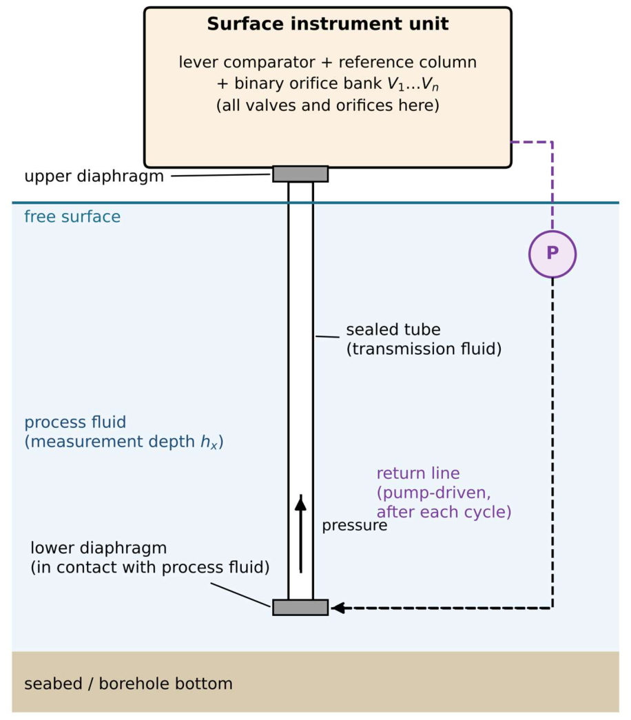
Two further architectural recommendations follow for a field-deployed version of this instrument, illustrated in Figure 5. First, hydrostatic pressure should be transmitted from the seabed (or borehole bottom) to the instrument via a dedicated transmission tube fitted with a diaphragm at each end, rather than by extending the orifice bank itself down to the measurement point: the lower diaphragm, in direct contact with the process fluid at the point of measurement, isolates the process side from the transmission fluid, while the upper diaphragm, at the instrument end, transmits the resulting pressure to the reference-column/orifice-bank assembly. This keeps every calibrated orifice and the comparator mechanism within a single controlled, accessible unit at the surface (or an easily serviceable enclosure), and confines the binary-search measurement itself, including all valves and orifices, to that unit rather than requiring it to operate at depth. Second, because each binary-search measurement admits a small, calibrated volume of fluid into the reference column (Section 3.6), repeated measurement cycles in the field require this fluid to be returned rather than allowed to accumulate: at the end of each cycle, the excess reference-column fluid should be pumped back, via a dedicated return line, to the diaphragm at the process end, and all valves closed, before the next cycle begins. This closed-loop recirculation keeps the total fluid inventory constant across repeated measurements and restores the reference column to its initial state without requiring an external fluid supply or drain at the deployment site.
Figure 5.
Recommended field-deployment architecture: a diaphragm-sealed transmission tube isolates the process fluid at the measurement point from the instrument, keeping the comparator and orifice bank of Figs. 1 and 3 in a single accessible unit; a pump-driven return line recirculates excess fluid to the process-end diaphragm after each measurement cycle, closing the loop without an external fluid supply or drain.
Figure 5.
Recommended field-deployment architecture: a diaphragm-sealed transmission tube isolates the process fluid at the measurement point from the instrument, keeping the comparator and orifice bank of Figs. 1 and 3 in a single accessible unit; a pump-driven return line recirculates excess fluid to the process-end diaphragm after each measurement cycle, closing the loop without an external fluid supply or drain.
Finally, we state plainly a constraint on the present work: the author is an independent researcher without institutional affiliation, a research budget, or fabrication facilities, and has not constructed the physical apparatus described in this paper. Every quantitative claim above the level of arithmetic and simulation — the channel dimensions of Table 1, the δd = 1 μm dimensional-stability assumption of Section 3.4, and the error figures of Table 3 and Table 4 — rests on the physical modelling and Monte Carlo simulation described herein, not on physical measurement. This paper is accordingly offered as a fully specified design and error analysis, together with an executable validation protocol (Section 3.7 and Section 3.8), rather than as a report of a built and tested instrument. Constructing the apparatus and executing the proposed 40-point validation is left as an explicit direction for future work, to be carried out either by the author, should resources become available, or by other researchers with access to the necessary machining and metrology equipment.
7. Conclusion
This paper presented a hydromechanical binary-search architecture in which hydrostatic pressure is converted to an n-bit digital code using individually calibrated, laminar-flow binary-pressure orifices and a purely mechanical lever comparator, without any electrical sensing element. A Monte Carlo simulation of the complete manual procedure, using a physically-derived, bit-dependent calibration-retention error model, identified orifice calibration retention as the dominant error source and established a practical operating point of n = 10 bits, giving an effective resolution of approximately 1.4 mm (ENOB ≈ 7.7) over a 1.024 m bench-scale range. The architecture extends our prior demonstration that the successive-approximation principle is independent of the specific physical quantity involved [5,6], showing here that it is also independent of the electrical domain altogether.
Data availability: The Monte Carlo simulation code used to generate Table 3 and Table 4 and Figure 4, together with the seeded generation script for the 40-point target-value list of Table 2, is available from the author on reasonable request (mohsensbu@gmail.com). As detailed in Section 3.8 and Section 6, no physical apparatus has been constructed at the time of writing; no experimental readings exist beyond the simulated and computed quantities reported in this paper.
Declaration of generative AI and AI-assisted technologies in the manuscript preparation process: During the preparation of this work, the author used Claude (Anthropic) to generate the Monte Carlo simulation code and to produce an initial draft of the manuscript text. All research ideas, methodological decisions, and the overall direction of the work were conceived and directed entirely by the author, who reviewed, verified, and edited all AI-generated content and takes full responsibility for the content of the published article.
References
- Fibonacci, L. Liber Abaci (1202), “On IIII Weights Weighing Forty Pounds,” as discussed in secondary sources on the history of the binary-weighing problem.
- Bachet de Méziriac, C.-G. Problèmes plaisants et délectables qui se font par les nombres, 2nd ed.; Lyon, 1624. [Google Scholar]
- Hardy, G.H.; Wright, E.M. An Introduction to the Theory of Numbers; Oxford University Press: Oxford, U.K.
- Murmann, B. The successive approximation register ADC: a versatile building block for ultra-low-power to ultra-high-speed applications. IEEE Commun. Mag. 2016, vol. 54(no. 4), 78–83. [Google Scholar] [CrossRef]
- Karimi, M. A shared binary intensity-search architecture for multi-sensor ADC-less sensing with two-peak telemetry. Preprints.org preprint ID 241626. 2026. [Google Scholar]
- Karimi, M. Significance-weighted tolerance allocation for binary-weighted measurement systems built from discrete components: a closed-form rule and its validity boundary. Preprints.org. preprint ID 241645. 2026. [Google Scholar]
- Hydrostatic sensor device and method for measuring below-ground elevation changes in grade. U.S. Patent 8,061,050.
- Level measurement method using measurements of water column pressure therefor. U.S. Patent 5,791,187.
- Khan; Mishra, S.; Pandey, S.; Sardar, T.; Mishra, A.; Mudgal, M.; Singhai, S. A critical review of IoT-based structural health monitoring for dams. IEEE Internet Things J. 2025, vol. 12(no. 2), 1368–1379. [Google Scholar] [CrossRef]
- Höttges; Rabaiotti, C.; Facchini, M. A novel distributed fiber-optic hydrostatic pressure sensor for dike safety monitoring. IEEE Sens. J. 2023, vol. 23(no. 23), 28942–28953. [Google Scholar] [CrossRef]
- Method and measuring device for measuring hydrostatic pressure, in particular that of ground water. U.S. Patent 5,983,716.
- Pineau-Guillou, L.; Lazure, P. A high-frequency dataset of sea level observations from low-cost pressure sensors. Sci. Data 2025, vol. 12, art. 999. [Google Scholar] [CrossRef] [PubMed]
- Zavei-Boroda; Minear, J.T.; Harlow, K.; Woods, D.; Heckman, C. Cost-Effective Radar Sensors for Field-Based Water Level Monitoring with Sub-Centimeter Accuracy. arXiv 2026, arXiv:2601.03447. [Google Scholar] [CrossRef]
- Yue, W.; Guo, Y.; Lee, J.-C.; Ganbold, E.; Wu, J.-K.; Li, Y.; Wang, C.; Kim, H.S.; Shin, Y.-K.; Liang, J.-G.; Kim, E.-S.; Kim, N.-Y. Advancements in passive wireless sensing systems in monitoring harsh environment and healthcare applications. Nano-Micro Lett. vol. 17, 106, 2025. [CrossRef] [PubMed]
- Moser, M.; Pradhan, M.; Emal, I.U.H.; Bastia, S.; Kaschel, M.; Edelmann, K.; Kallfass, I.; Burghartz, J.N. Low-power AlGaN/GaN pressure sensors for harsh environmental conditions with high sensitivity. Power Electron. Devices Compon. vol. 10, art. 100076, 2025. [CrossRef]
- Loizou, K.; Koutroulis, E. Water level sensing: state of the art review and performance evaluation of a low-cost measurement system. Measurement 2016, vol. 89, 204–214. [Google Scholar] [CrossRef]
- White, F.M. Fluid Mechanics; McGraw-Hill.
Table 1.
Laminar-orifice design parameters (L = 100 mm, Re = 1000, water, n = 12).
| Bit (i) | ΔP_i (Pa) | d_i (mm) | Q_i (mL/s) | V_i (mL) | Fill time |
|---|---|---|---|---|---|
| 1 (MSB) | 5023 | 0.86 | 0.676 | 90.5 | 134 s |
| 2 | 2511 | 1.08 | 0.852 | 45.2 | 53 s |
| 3 | 1256 | 1.37 | 1.073 | 22.6 | 21 s |
| 4 | 628 | 1.72 | 1.352 | 11.3 | 8.4 s |
| 5 | 314 | 2.17 | 1.703 | 5.65 | 3.3 s |
| 6 | 157 | 2.73 | 2.146 | 2.83 | 1.3 s |
| 7 | 78.5 | 3.44 | 2.703 | 1.41 | 0.52 s |
| 8 | 39.2 | 4.34 | 3.406 | 0.71 | 0.21 s |
| 9 | 19.6 | 5.46 | 4.291 | 0.35 | 0.08 s |
| 10 | 9.81 | 6.88 | 5.407 | 0.18 | 0.033 s |
| 11 | 4.91 | 8.67 | 6.812 | 0.088 | 0.013 s |
| 12 (LSB, n=12) | 2.45 | 10.93 | 8.582 | 0.044 | 0.005 s |
Table 3.
Isolated contribution of each error source (n = 12 bits, L = 100 mm, δd = 1 μm, 20,000-trial Monte Carlo).
Table 3.
Isolated contribution of each error source (n = 12 bits, L = 100 mm, δd = 1 μm, 20,000-trial Monte Carlo).
| Source | RMSE (mm) |
|---|---|
| Orifice calibration retention (σ_manuf,i, bit-dependent) | 1.39 |
| Differential density mismatch (σ = 0.02%) | 0.14 |
| Pivot friction / hysteresis deadband | 0.10 |
| Ideal quantization only (no non-idealities) | 0.07 |
| All sources combined | 1.40 |
Table 4.
Resolution and effective number of bits (ENOB) vs. nominal bit count (L = 100 mm, δd = 1 μm).
Table 4.
Resolution and effective number of bits (ENOB) vs. nominal bit count (L = 100 mm, δd = 1 μm).
| n | Ideal ΔH (mm) | Ideal floor (mm) | Simulated RMSE (mm) | ENOB |
|---|---|---|---|---|
| 6 | 16.000 | 4.619 | 4.80 | 5.95 |
| 8 | 4.000 | 1.155 | 1.80 | 7.36 |
| 9 | 2.000 | 0.577 | 1.48 | 7.64 |
| 10 | 1.000 | 0.289 | 1.40 | 7.73 |
| 11 | 0.500 | 0.144 | 1.39 | 7.73 |
| 12 | 0.250 | 0.072 | 1.36 | 7.77 |
| 14 | 0.0625 | 0.018 | 1.37 | 7.76 |
Disclaimer/Publisher’s Note: The statements, opinions and data contained in all publications are solely those of the individual author(s) and contributor(s) and not of MDPI and/or the editor(s). MDPI and/or the editor(s) disclaim responsibility for any injury to people or property resulting from any ideas, methods, instructions or products referred to in the content. |
© 2026 by the authors. Licensee MDPI, Basel, Switzerland. This article is an open access article distributed under the terms and conditions of the Creative Commons Attribution (CC BY) license (http://creativecommons.org/licenses/by/4.0/).
Copyright: This open access article is published under a Creative Commons CC BY 4.0 license, which permit the free download, distribution, and reuse, provided that the author and preprint are cited in any reuse.