
Submitted:
31 October 2026
Posted:
03 November 2026
You are already at the latest version
Abstract
Calibration remains a practical barrier for steady-state visual evoked potential (SSVEP) brain–computer interfaces. Task-related component analysis (TRCA) is accurate when several labelled trials per class are available, but its performance degrades when calibration is reduced to one trial and the test block follows a change in recording conditions. We asked whether a fixed modification of ensemble TRCA (eTRCA) could reduce this loss without any per-subject hyperparameter tuning. The proposed SST-eTRCA appends a three-sample delayed copy of each channel, z-scores observations before covariance accumulation, and pools 80 class filters into one projection. On the public 35-subject Tsinghua benchmark (40 classes, six posterior channels), it reached 95.6% with one calibration trial per class versus 93.4% for eTRCA (1400 decisions; McNemar p = 1.5E-5), and 95.0% versus 91.8% without extra calibration. The advantage was largest at 1 s (68.9% versus 63.9%). Under leave-one-subject-out, SST-eTRCA and eTRCA were indistinguishable (83.6% each), and self-training changed accuracy by only 0.1 points (p = 0.75). The gain is therefore specific to within-participant block shift, not to cross-subject transfer. These results define a narrow but useful operating range: a fixed, reproducible decoder for reducing recalibration across blocks, with the negative self-training result serving as a reliability check.
Keywords:
steady-state visual evoked potentials
; brain–computer interface
; task-related component analysis
; calibration reduction
; covariance conditioning
; cross-subject generalization
1. Introduction
Steady-state visual evoked potentials (SSVEPs) are periodic cortical responses to flickering stimuli and remain one of the most practical control signals for non-invasive brain–computer interfaces (BCIs) [1,2]. Because the response is narrow-band and phase-locked to the stimulus, target identification reduces to frequency detection, and correlation-based decoders have shaped the field for two decades. Canonical correlation analysis (CCA) between the multichannel electroencephalogram (EEG) and sine–cosine references [3,4] was followed by filter-bank CCA [5], multiset CCA [6] and individual-template variants [7], and these methods still provide the reference point against which newer decoders are judged.
Task-related component analysis (TRCA) replaced the reference signals with spatial filters estimated from the user’s own calibration trials [8]. The filters maximise the reproducibility of a task-related component across trials of the same class, so the decoder adapts to the individual scalp distribution of the response. Its ensemble extension, eTRCA, concatenates the filters of every class and sums the resulting correlations [9]. With a few seconds of stimulation and a short calibration session, eTRCA exceeds 90 % accuracy on 40-class benchmarks [10], which is why it underpins most high-speed spellers [11].
Calibration cost is one constraint. A TRCA-type decoder needs several labelled trials per class, and accuracy falls steeply when only one or two are available [12]. Stationarity is the other. Even with adequate calibration, the covariance structure of the EEG changes between blocks and between sessions, through electrode impedance, fatigue, posture and attention. A decoder fitted on one block therefore loses accuracy on the next, and the loss is largest for the linear filters that depend on a well-conditioned covariance estimate.
A large literature addresses both problems. Transfer-learning designs borrow trials or templates from other subjects [13,14,15], regress responses across stimuli [16], or align covariance matrices in a Euclidean reference space [17]. Hybrid schemes combine task-related and canonical correlation objectives [18], or pair task-related filters with a convolutional network [19], and channel or subspace selection reduces the number of parameters that have to be estimated from limited data [20]. Deep networks learn the spatial filters end to end [21,22], and recent reviews discuss their performance and data requirements [23,24]. Spectrum-enhanced TRCA (SE-TRCA) appends shifted copies of the signal as extra channels, which supplies the covariance estimate with temporal context [25]. Transductive self-training is often added on top, on the assumption that unlabelled test trials can be relabelled and folded back into the templates.
Three issues cut across this literature. Reported gains are frequently attributed to the classifier or to the fusion rule, while the conditioning of the covariance estimate, which every TRCA variant depends on, is left unexamined. Comparisons are often run on a single corpus, so it is unclear whether a gain reflects within-subject adaptation or a better cross-subject representation. And self-training is usually assumed to help, with little reporting of the cases in which it does not.
This paper asks whether a fixed decoder modification can reduce recalibration without per-subject tuning. The decoder, which we call SST-eTRCA, keeps the eTRCA scoring rule and changes three things: a single three-sample lag is appended to the channel set, each observation is z-scored before the covariance is accumulated, and the per-class filters are pooled into one projection that is applied to every trial. All three choices are fixed in advance and applied unchanged to all 35 participants. We report a held-out-block protocol with zero or one calibration trial per class, a leave-one-subject-out protocol on the same decoder, a window sweep from 0.5 s to 5 s, a self-training on/off comparison, and an ablation of the three design choices.
The central result is a boundary, not a universal gain. With one calibration trial per class, SST-eTRCA reaches 95.6 % on the held-out block against 93.4 % for eTRCA, and the advantage holds at every window length we tested. Under leave-one-subject-out the same decoder is statistically indistinguishable from eTRCA and SE-TRCA (83.6 % each against eTRCA). The gain is therefore specific to within-participant block shift and does not transfer to unseen participants. Self-training changes accuracy by only 0.1 points (); we retain this null result as a reliability check rather than tuning it away.
The contributions are as follows.
- A fixed three-part modification of eTRCA that requires no per-subject hyperparameter search and no gradient-based training.
- A public 35-subject, 40-class evaluation in which the decoder reaches 95.6 % with one calibration trial per class, compared with 93.4 % for eTRCA.
- A boundary result: leave-one-subject-out accuracy is indistinguishable from eTRCA (83.6 % each), which locates the benefit in within-participant block shift rather than cross-subject transfer.
- A negative self-training result, together with the ablation and parameter budget, which serves as a reliability check on the operating range of the decoder.
2. Materials and Methods
2.1. Public Benchmark
We used the SSVEP benchmark released by Wang et al. [10], which is public and de-identified. Thirty-five participants performed a 40-target spelling task with stimuli modulated between 8 Hz and 15.8 Hz. Each participant completed six blocks of 40 trials, one trial per target per block, giving 240 trials per participant and 8400 trials in total. The signals were recorded at 1000 Hz and released downsampled to 250 Hz.
We retained six posterior channels (CP3, CPZ, CP4, PO3, POZ, PO4) and the stimulation window from 0.5 s to 5.5 s after stimulus onset, which gives 1250 samples per trial. The chance level is 1/40, or 2.5 %. No artefact rejection was applied beyond the filtering described in Section 2.3.
The study used only publicly released, de-identified benchmark data. No new participants were recruited and no new data were collected. Use of the data follows the original release terms.
2.2. Evaluation Protocols
- Held-out block.
Blocks 0–3 form the training set, with four labelled trials per class. Block 4 supplies additional calibration trials, and block 5 is held out and decoded once per condition. Because block 4 contains exactly one trial per class, the calibration budget k can only take the values 0 and 1; larger budgets cannot be formed from this benchmark without reusing training trials, and we do not report them. Every method is evaluated on decisions per condition.
We stress what means here. The decoder is still fitted on the 160 labelled trials of blocks 0–3. The label refers to the absence of an additional calibration block, not to a data-free decoder. We use the phrase “without extra calibration” for this condition throughout.
- Leave-one-subject-out.
For each held-out participant, the source pool contains the training blocks of the other 34 participants, and the test set is the held-out participant’s block 5. Two conditions are formed: without calibration, and with the held-out participant’s block 4 added to the source pool at one trial per class. No trial from the held-out participant’s test block enters training, and the source pool is rebuilt for each fold with that participant removed.
- Window sweep.
The same held-out-block protocol is repeated with stimulation windows of 0.5, 1, 1.5, 2, 3, 4 and 5 s. The filters and templates are re-estimated at each window length from the corresponding prefix of each trial.
A held-out block is not a new recording session. It is the closest controlled approximation that this benchmark supports, since all six blocks were recorded in one visit but separated in time, and the electrode cap was not re-applied between them. We describe results from this protocol as held-out-block results and avoid the word session where the distinction matters.
2.3. Preprocessing
Each trial is z-scored channel by channel, filtered with a fourth-order Butterworth band-pass (0.02–0.15 cycles per sample, applied forward and backward to avoid phase distortion), and z-scored again. The second z-scoring restores unit variance after the filter has removed most of the power. The same function is used for training, for self-training and for inference; a mismatch between these three paths would silently shift the feature distribution.
2.4. Filter Bank and Shared Projection
Let collect the training trials of class c, each of dimension T. TRCA seeks a spatial filter that maximises the reproducibility of the projected signal across trials,
where is the inter-trial covariance sum and is the pooled within-trial covariance. The solution is the leading eigenvector of , and we retain the two leading eigenvectors per class ().
Before is accumulated, each observation is z-scored across time. This is the normalisation choice that distinguishes the present decoder from the centred covariance used by the eTRCA baseline, and it makes invariant to a constant gain applied to any channel. It does not make the filters invariant to a change of noise colour, which is why the band-pass stage still matters.
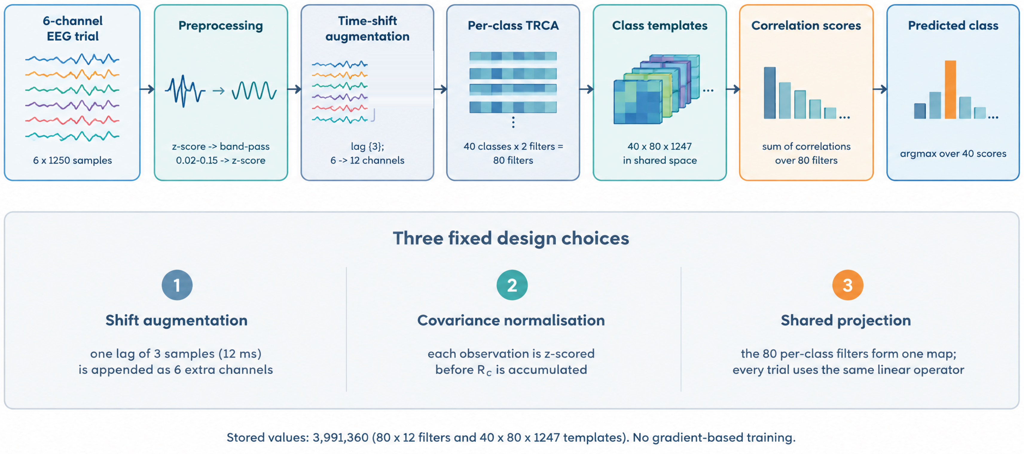
The channel set is expanded before the filters are estimated. A copy of the trial delayed by samples (12 ms at 250 Hz) is appended along the channel axis,
so six electrodes become twelve channels and the trial shortens to 1247 samples. The delayed copy carries no new information about the stimulus, but it changes the covariance structure that the eigenproblem sees: the cross-covariance between a channel and its delayed self enters , and the filters can exploit the temporal correlation of the SSVEP over one stimulus cycle.
With 40 classes and two filters each, the bank contains 80 filters. In the ensemble formulation these are concatenated into a single projection , and every trial, whatever its class, is projected through the same map. Class templates are the mean projected trial of each class in that 80-dimensional space, .
Figure 1.
Architecture of the proposed decoder. A six-channel trial is z-scored, band-pass filtered and augmented with a three-sample delayed copy. Per-class TRCA filters are pooled into one projection, and the class score is the sum of correlations against the class templates. The lower panel isolates the three fixed design choices. The decoder stores 3 991 360 values and uses no gradient-based training.
Figure 1.
Architecture of the proposed decoder. A six-channel trial is z-scored, band-pass filtered and augmented with a three-sample delayed copy. Per-class TRCA filters are pooled into one projection, and the class score is the sum of correlations against the class templates. The lower panel isolates the three fixed design choices. The decoder stores 3 991 360 values and uses no gradient-based training.
2.5. Score Vector and Readout
For a test trial , the projection is , and the score of class c is the sum of Pearson correlations between corresponding rows of and ,
The predicted label is . The rule has no trainable parameters: the templates are means, and the argmax introduces nothing to fit. We use the same score vector for the self-training stage described next.
2.6. Transductive Self-Training
Self-training relabels the unlabelled test trials with the current model and refits the templates on the union of labelled and pseudo-labelled trials. We run three rounds. In each round the model scores the test block, keeps the 75 % most confident predictions per class, adds them to the template set, and recomputes the class means. The filters are not re-estimated, so the loop changes the templates only. Rounds are applied identically to every method in the comparison, and Section 3.4 reports what they buy.
2.7. Baselines
Four decoders are re-implemented in the same code base and evaluated on identical splits.
- CCA [3]: canonical correlation between the six-channel trial and sine–cosine references at the stimulus frequency and its harmonics. The number of harmonics is selected from on the labelled training blocks. Band-pass 0.02–0.15 cycles per sample.
- TRCA [8]: per-class filters with , centred covariance, no shift augmentation, argmax over class scores.
- eTRCA [9]: identical to TRCA except that the 80 filters are pooled into one projection, which is the direct parent of the proposed reader.
- SE-TRCA [25]: our re-implementation, with one shift tap, filters per class and per-class scoring. The original report used a different recording set-up, so the numbers here are not directly comparable with the published ones; the comparison is between implementations under one protocol.
All four use the same pre-processing function, the same training blocks and the same calibration trials as the proposed reader.
2.8. Parameter Budget
Table 1 lists the stages of the reader with the number of values each stores. The reader holds 3 991 360 values, of which 3 990 400 are template entries. The filters account for 960 values. Nothing in the pipeline is trained by gradient descent, and the templates are means rather than fitted parameters.
2.9. Statistical Analysis
Accuracy is reported as the pooled proportion over all decisions, with a Wilson score interval. Because decisions are paired across methods, we use the exact McNemar test on the discordant pairs, and we report b (reference correct, competitor wrong) and c (the reverse) alongside the p value. Subject-level comparisons use the Wilcoxon signed-rank test on the 35 per-subject accuracy differences. Both families of tests are corrected with the Holm procedure [26] within each budget condition. We report uncorrected and corrected values.
Information transfer rate follows the standard definition for a selection task with N equiprobable targets,
with , accuracy P, and s. The 6 s analysis time is the 5 s stimulation window plus a 1 s inter-trial interval, so the reported rates correspond to a complete trial cycle rather than to the stimulation window alone. Rates computed with s would be about 20 % higher and are not used anywhere in this paper.
3. Results
3.1. Accuracy on the Held-Out Block
Table 2 gives accuracy and ITR for the five decoders, without extra calibration and with one trial per class. The proposed reader reaches 95.0 % and 95.6 % respectively. The ordering of the baselines is the one usually reported for this benchmark: eTRCA above SE-TRCA, SE-TRCA above TRCA, and CCA far below the three spatial-filtering methods. The gap between the reader and its direct parent eTRCA is 3.2 points without extra calibration and 2.2 points with one trial per class.
Figure 2.
Accuracy and ITR on the held-out block for the five decoders, with and without one calibration trial per class. Bars are means over 35 participants and whiskers are standard errors of the mean. The proposed reader leads at both budgets; the distance to eTRCA is smaller than the between-participant spread.
Figure 2.
Accuracy and ITR on the held-out block for the five decoders, with and without one calibration trial per class. Bars are means over 35 participants and whiskers are standard errors of the mean. The proposed reader leads at both budgets; the distance to eTRCA is smaller than the between-participant spread.
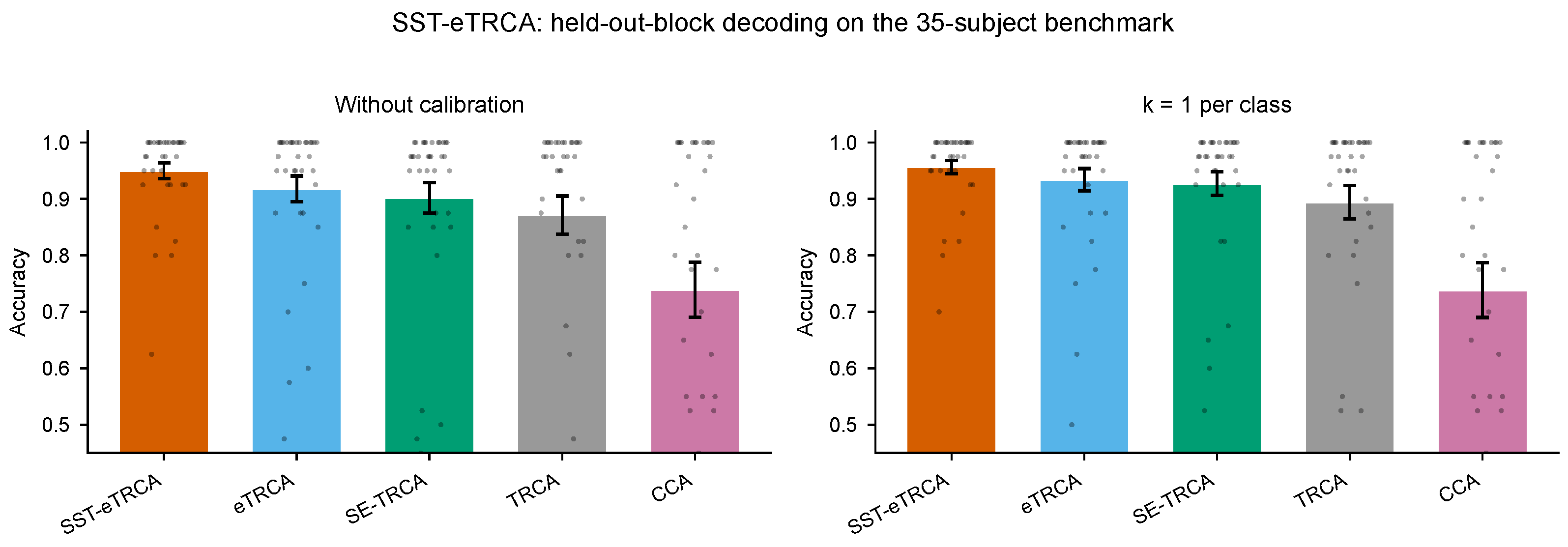
Paired tests confirm that the ordering is not a pooling artefact. With one calibration trial per class, the reader is correct on 41 decisions that eTRCA misses and wrong on 10 that eTRCA gets right (McNemar ; Holm-corrected ). Against SE-TRCA the discordant counts are 60 and 19 (), against TRCA 98 and 11, and against CCA 318 and 13. Without extra calibration the corresponding counts against eTRCA are 52 and 7 (). The subject-level Wilcoxon test agrees at both budgets: without calibration and with one trial per class, both surviving Holm correction within their family.
Table 3 collects the full set of comparisons.
3.2. Participant-Level Spread
Pooled accuracy hides how the gain is distributed. Figure 3 shows per-participant accuracy for the reader against each baseline at one calibration trial per class. Most points sit above the diagonal, which is consistent with the discordant counts, but the margin varies: participants who are already near 100 % with eTRCA have little room to improve, and the largest gains appear among participants in the 85–95 % band. The mean per-participant difference against eTRCA is 2.2 points with a standard deviation of 5.4, so the advantage is a modest shift of the distribution rather than a rescue of a few failing participants.
3.3. Where the Residual Errors Fall
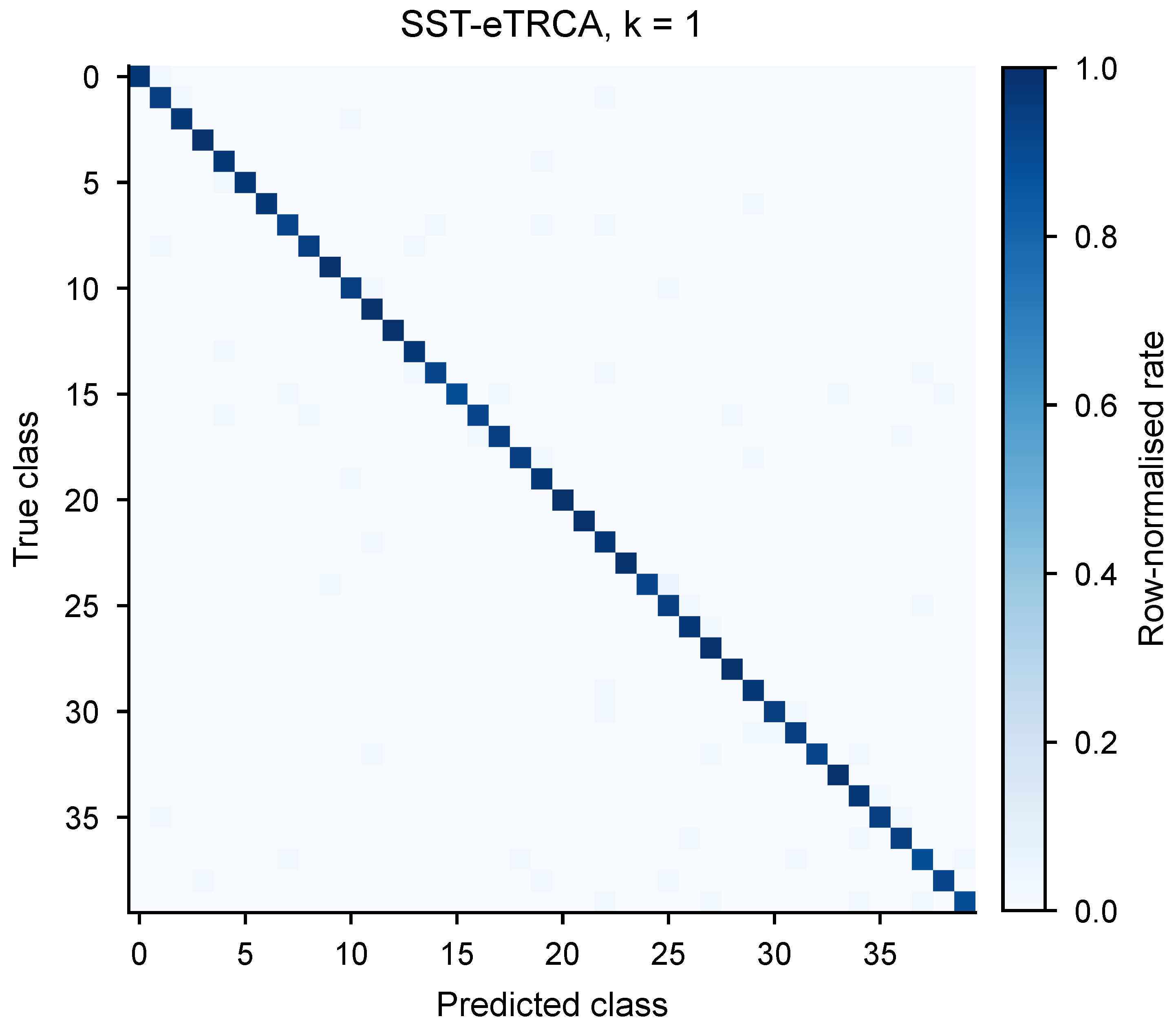
The reader makes 61 errors in 1400 decisions. Per-class recall ranges from 88.6 % to 100 %, with a median of 97.1 %, and three classes fall below 90 % (classes 15, 37 and 39, using zero-based indices in the order of increasing stimulus frequency). The only repeated off-diagonal pair is 24 → 25, which occurs twice; every other error is a single trial. Most of the remaining errors sit between neighbouring frequencies, which is what a correlation-based decoder with a 5 s window would be expected to produce when the signal-to-noise ratio is low. Errors between distant targets are rare.
Figure 4.
Confusion matrix of the reader on the pooled held-out block at one calibration trial per class (1400 decisions, 61 errors). Rows are true classes and columns predicted classes, ordered by stimulus frequency. The dominant off-diagonal entries sit next to the diagonal.
Figure 4.
Confusion matrix of the reader on the pooled held-out block at one calibration trial per class (1400 decisions, 61 errors). Rows are true classes and columns predicted classes, ordered by stimulus frequency. The dominant off-diagonal entries sit next to the diagonal.
3.4. What Self-Training Adds
Table 4 compares each decoder with and without three rounds of transductive self-training. For the proposed reader the change is +0.1 points at one calibration trial per class and points without extra calibration; the exact McNemar tests give and . Neither difference is distinguishable from zero. The same step slightly reduces accuracy for eTRCA, SE-TRCA and TRCA at both budgets.
This is a null result and we report it as such. On a 40-class problem where the seed model is already correct on 95.6 % of trials, the pool of confidently mislabelled trials is small, and three rounds of template refitting cannot move the decision boundary much. Whether self-training helps therefore depends on the seed accuracy rather than on the algorithm alone. Section 4 returns to this point.
3.5. Decoding Window
Figure 5 and Table 5 report accuracy at seven window lengths with one calibration trial per class. The reader is ahead of eTRCA at every length. The absolute advantage is 4.1 points at 0.5 s, 5.0 at 1 s, 3.6 at 1.5 s, 2.9 at 2 s, 3.5 at 3 s, 2.6 at 4 s and 2.2 at 5 s. The largest absolute gain is at 1 s, where the reader reaches 68.9 % against 63.9 %.
The ITR curves in Figure 5 peak near 1.5–2 s for all methods, well below the 5 s window that maximises accuracy. That peak is a property of the ITR formula, which divides by the decision time, and not evidence that short windows decode better. We report both quantities because the choice of window in a real speller depends on which one the application values.
3.6. Cross-Subject Generalisation
Table 6 and Figure 6 give leave-one-subject-out results. The reader reaches 83.6 % with one calibration trial per class, exactly the value obtained by eTRCA and SE-TRCA. Without calibration the three are 83.4 %, 82.6 % and 82.9 %, a spread of less than one point. All three exceed TRCA (80.9 %) and CCA (74.4 %), so the ensemble construction and the shift augmentation both help relative to per-class filtering, but they do not separate from each other.
This result constrains the interpretation of Section 3.1. A change that adds two points when the test block comes from the same participant adds nothing when it comes from a different one. Whatever the shift augmentation and the covariance normalisation do, they do it within a participant.
3.7. Ablation of the Design Choices
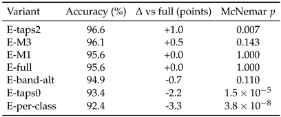
Table 7 removes one design choice at a time, keeping the protocol and the calibration budget fixed at one trial per class. The configuration was frozen before the benchmark was decoded, so this is a sensitivity analysis and not a selection procedure: we did not adopt any variant on the strength of its score here.
Two results dominate. Replacing the shared projection with per-class scoring costs 3.3 points (92.4 %, McNemar ), which makes the pooling of the 80 filters the largest single contributor. Removing the shift augmentation costs 2.2 points (93.4 %, ). Both changes act on the covariance estimate, which is the reading developed in Section 4.1.
The other variants move accuracy by less than a point, and most of them move it upwards. Two shift taps instead of one give 96.6 % (, ), three filters per class give 96.1 % (, ), one filter per class leaves the result unchanged, and the alternative pass-band costs 0.7 points. The reader is therefore not at a sharp optimum, and a further point is available by augmenting more. We did not take it. Choosing a configuration because it scores well on the test block would undo the point of the fixed recipe, and the headline figure of 95.6 % is one point below what the same architecture reaches with two taps. Reporting the gap seems more useful than closing it.
4. Discussion
4.1. The Gain Is a Covariance Effect
The two changes that separate the reader from eTRCA act on the same object. The shift augmentation changes the dimension of the covariance matrices in Equation 1 from to , and the z-scoring changes what those matrices contain: correlations rather than raw second moments. Both make the eigenproblem better conditioned when the number of trials per class is small, which is the regime that the one-trial calibration condition creates. A better-conditioned estimate produces filters that are less sensitive to the particular trials used to fit them, and templates that are more stable across blocks.
Two observations support this reading. The advantage is widest at short windows, where the covariance estimate is built from fewer samples and is therefore noisier. And the advantage is absent under leave-one-subject-out, where the filters are estimated from 136 trials per class drawn from 34 participants and conditioning is no longer the limiting factor. If the reader had found a richer representation of the SSVEP, the cross-subject result should have improved as well.
4.2. Why the Cross-Subject Result Is Informative
It would be convenient to present the held-out-block gain as evidence of general robustness. The leave-one-subject-out result does not support that reading, and we prefer to state the boundary explicitly. The reader is a within-participant decoder. It reduces the cost of re-calibrating a participant whose signal has drifted, and it does nothing for a participant from whom no labelled trial has been collected.
In deployment, a speller used by one person over several sessions benefits from a decoder that tolerates a change of block without new labels, and the 95.6 % figure applies. In a plug-and-play setting, where a new user has to be served without calibration, the relevant number is the 83.6 % from Table 6, and the reader offers no improvement over eTRCA. Applications should be matched to the appropriate column.
4.3. Relation to Prior Work
SE-TRCA also augments the channel set with delayed copies [25], and our shift stage follows that idea. The difference is in what the augmentation is combined with. SE-TRCA retains per-class scoring with four filters per class, while the present reader pools 80 filters into one projection and normalises each observation before the covariance is formed. Under our protocol the pooled version is ahead of the per-class version at every window length, which suggests that the sharing matters as much as the augmentation. We cannot separate the two contributions from the published SE-TRCA results, because those were obtained on a different recording set-up.
The transfer-learning literature addresses a different problem [13,14,15,16]. Those methods move information between participants, and their natural evaluation is the subject-disjoint one. Methods that align covariance matrices [17] sit between the two regimes: they reduce session and subject differences with a shared reference, and they would be a sensible complement to the present reader, since the two act on different parts of the pipeline.
Deep decoders [21,22] replace the spatial filters with learned layers. They remove the conditioning problem by removing the eigenproblem, at the cost of parameters and training data. The reader described here sits at the other end: 3.99 million stored values, almost all of them templates, and no gradient training. For a 40-class problem with six channels, that is enough.
4.4. Limitations
The study has four limitations. All results come from one benchmark, recorded with one amplifier, one montage and one stimulus design, so the absolute numbers should not be transferred to other systems without re-testing. The held-out block is not a new session; it is a later block of the same recording, and a true session shift would include cap re-application and a change of electrode impedance. The claim in Section 4.1 is an inference from the pattern of results rather than a direct measurement of covariance conditioning, and a study that manipulated impedance directly would test it more sharply. Finally, only two calibration budgets are available from this benchmark, so the shape of the accuracy-versus-budget curve above one trial per class is not observed here.
5. Conclusions
We examined whether a fixed modification of ensemble TRCA improves SSVEP decoding when calibration is scarce. On a 35-subject, 40-class public benchmark, SST-eTRCA raised held-out-block accuracy from 93.4 % to 95.6 % with one calibration trial per class, and from 91.8 % to 95.0 % without extra calibration. The same decoder was indistinguishable from eTRCA under leave-one-subject-out (83.6 % each), and self-training changed accuracy by only 0.1 points. These results support a deliberately narrow claim: the method is a fixed, reproducible decoder for reducing recalibration across blocks, not a solution for cross-subject transfer. Reporting the negative self-training result and the leave-one-subject-out boundary alongside the positive within-participant result makes that operating range explicit.
Author Contributions
Wanli Wang: conceptualization, methodology, software, formal analysis, supervision, funding acquisition, writing—original draft and review and editing. Xiaoxue Su: software, validation and visualization. Xue Chen: investigation and data curation. Huafeng Chen: investigation and validation. Yangxi Zhang: visualization and writing—review and editing. All authors have read and agreed to the published version of the manuscript.
Funding
This work was supported by the Hubei Provincial Natural Science Foundation Program Project (No. 2026AFC0728) and the Hubei Provincial Department of Education Scientific Research Plan (No. B2024210).
Institutional Review Board Statement
Not applicable. This study is a secondary analysis of the publicly released, de-identified Tsinghua SSVEP benchmark. No new human participants were recruited and no new neural data were recorded.
Informed Consent Statement
Not applicable. No new human participants were recruited for this study; reuse of the benchmark is governed by its original release terms.
Data Availability Statement
The SSVEP benchmark analysed in this study is publicly available at https://doi.org/10.1109/TNSRE.2016.2627556 [10]. The processed per-trial outputs and the analysis code that produced every number and figure in this article are available from the corresponding author on reasonable request.
Acknowledgments
The authors thank the providers of the public SSVEP benchmark for releasing their recordings, and the participants of the original study.
Conflicts of Interest
The authors declare no conflicts of interest. The funders had no role in the design of the study; in the collection, analyses, or interpretation of data; in the writing of the manuscript; or in the decision to publish the results.
Abbreviations
The following abbreviations are used in this manuscript:
| SSVEP | Steady-state visual evoked potential |
| TRCA | Task-related component analysis |
| eTRCA | Ensemble task-related component analysis |
| CCA | Canonical correlation analysis |
| LOSO | Leave-one-subject-out |
| ITR | Information transfer rate |
References
- Cheng, M.; Gao, X.; Gao, S.; Xu, D. Design and implementation of a brain-computer interface with high transfer rates. IEEE Trans. Biomed. Eng. 2002, 49, 1181–1186. [Google Scholar] [CrossRef]
- Wolpaw, J.R.; Birbaumer, N.; McFarland, D.J.; Pfurtscheller, G.; Vaughan, T.M. Brain-computer interfaces for communication and control. Clin. Neurophysiol. 2002, 113, 767–791. [Google Scholar] [CrossRef]
- Lin, Z.; Zhang, C.; Wu, W.; Gao, X. Frequency recognition based on canonical correlation analysis for SSVEP-based BCIs. IEEE Trans. Biomed. Eng. 2006, 53, 2610–2614. [Google Scholar] [CrossRef]
- Bin, G.; Gao, X.; Yan, Z.; Hong, B.; Gao, S. An online multi-channel SSVEP-based brain-computer interface using a canonical correlation analysis method. J. Neural Eng. 2009, 6, 046002. [Google Scholar] [CrossRef]
- Chen, X.; Wang, Y.; Gao, S.; Jung, T.P.; Gao, X. Filter bank canonical correlation analysis for implementing a high-speed SSVEP-based brain-computer interface. J. Neural Eng. 2015, 12, 046008. [Google Scholar] [CrossRef]
- Zhang, Y.; Zhou, G.; Jin, J.; Wang, X.; Cichocki, A. Frequency recognition in SSVEP-based BCI using multiset canonical correlation analysis. Int. J. Neural Syst. 2014, 24, 1450013. [Google Scholar] [CrossRef]
- Nakanishi, M.; Wang, Y.; Wang, Y.T.; Jung, T.P. A comparison study of canonical correlation analysis based methods for detecting steady-state visual evoked potentials. PLoS ONE 2015, 10, e0140703. [Google Scholar] [CrossRef]
- Tanaka, T.; Katura, T.; Sato, H. Task-related component analysis for functional neuroimaging and application to near-infrared spectroscopy data. NeuroImage 2013, 64, 308–327. [Google Scholar] [CrossRef]
- Nakanishi, M.; Wang, Y.; Chen, X.; Wang, Y.T.; Gao, X.; Jung, T.P. Enhancing detection of SSVEPs for a high-speed brain speller using task-related component analysis. IEEE Trans. Biomed. Eng. 2018, 65, 104–112. [Google Scholar] [CrossRef] [PubMed]
- Wang, Y.; Chen, X.; Gao, X.; Gao, S. A benchmark dataset for SSVEP-based brain-computer interfaces. IEEE Trans. Neural Syst. Rehabil. Eng. 2017, 25, 1746–1752. [Google Scholar] [CrossRef]
- Chen, X.; Wang, Y.; Nakanishi, M.; Gao, X.; Jung, T.P.; Gao, S. High-speed spelling with a noninvasive brain-computer interface. Proc. Natl. Acad. Sci. 2015, 112, E6058–E6067. [Google Scholar] [CrossRef]
- Wong, C.M.; Wan, F.; Wang, B.; Wang, Z.; Nan, W.; Lao, K.F.; Mak, P.U.; Vai, M.I.; Rosa, A. Learning across multi-stimulus enhances target recognition methods in SSVEP-based BCIs. J. Neural Eng. 2020, 17, 016026. [Google Scholar] [CrossRef]
- Li, H.; Xu, G.; Li, Z.; Zhang, K.; Jiang, H.; Guo, X.; Zhu, Y.; Yang, X.; Zhao, Y.; Han, C. Inter- and intra-subject transfer learning for high-performance SSVEP-BCI with extremely little calibration effort. Expert Syst. With Appl. 2025, 276, 127208. [Google Scholar] [CrossRef]
- Luo, T.j. Dual-templates transferred canonical correlation analysis for cross-subject SSVEP-based BCIs. Expert Syst. With Appl. 2026, 302, 130611. [Google Scholar] [CrossRef]
- Xiong, H.; Chang, S.; Liu, J. Dual-channel TRCA-net based on cross-subject positive transfer for SSVEP-BCI. Biomed. Phys. Eng. Express 2025, 12, 015024. [Google Scholar] [CrossRef]
- Mai, X.; Meng, J.; Ding, Y.; Zhu, X.; Guan, C. SRRNet: unseen SSVEP response regression from stimulus for cross-stimulus transfer in SSVEP-BCIs. IEEE Trans. Neural Syst. Rehabil. Eng. 2025, 33, 1460–1472. [Google Scholar] [CrossRef]
- He, H.; Wu, D. Transfer learning for brain-computer interfaces: a Euclidean space data alignment approach. IEEE Trans. Biomed. Eng. 2020, 67, 399–410. [Google Scholar] [CrossRef]
- Besharat, A.; Samadzadehaghdam, N.; Ghadiri, T. A novel hybrid method based on task-related component and canonical correlation analyses (H-TRCCA) for enhancing SSVEP recognition. Front. Neurosci. 2025, 19, 1544452. [Google Scholar] [CrossRef]
- Wei, Q.; Li, C.; Wang, Y.; Gao, X. Enhancing the performance of SSVEP-based BCIs by combining task-related component analysis and deep neural network. Sci. Rep. 2025, 15, 365. [Google Scholar] [CrossRef]
- Li, H.; Xu, G.; Feng, S.; Du, C.; Han, C.; Kuang, J.; Zhang, S. Improving individual-specific SSVEP-BCI with adaptive channel and subspace selection in TRCA. Sensors 2026, 26, 1123. [Google Scholar] [CrossRef]
- Lawhern, V.J.; Solon, A.J.; Waytowich, N.R.; Gordon, S.M.; Hung, C.P.; Lance, B.J. EEGNet: a compact convolutional neural network for EEG-based brain-computer interfaces. J. Neural Eng. 2018, 15, 056013. [Google Scholar] [CrossRef] [PubMed]
- Klein, T.; Minakowski, P.; Sager, S. Flexible patched brain transformer model for EEG decoding. Sci. Rep. 2025, 15, 10935. [Google Scholar] [CrossRef] [PubMed]
- Yao, Y.; Wang, H.; Chen, L.; Peng, Y.; Luo, J. Foundation models for EEG decoding: current progress and prospective research. J. Neural Eng. 2025, 22, 061002. [Google Scholar] [CrossRef]
- Zhang, H.; Tao, C. Deep learning decoding of steady-state visual evoked potential (SSVEP) for real-time mobile brain–computer interfaces: a narrative review from laboratory settings to lightweight engineering applications. Brain Sci. 2026, 16, 387. [Google Scholar] [CrossRef]
- Mijani, A.; Norizadeh Cherloo, M.; Tang, H.; Zhan, L. Spectrum-Enhanced TRCA (SE-TRCA): a novel approach for direction detection in SSVEP-based BCI. Comput. Biol. Med. 2023, 166, 107488. [Google Scholar] [CrossRef]
- Holm, S. A simple sequentially rejective multiple test procedure. Scand. J. Stat. 1979, 6, 65–70. [Google Scholar]
Figure 3.
Per-participant accuracy at one calibration trial per class, proposed reader against each baseline. Each point is one of the 35 participants; the diagonal marks equal accuracy. Points above the diagonal favour the reader.
Figure 3.
Per-participant accuracy at one calibration trial per class, proposed reader against each baseline. Each point is one of the 35 participants; the diagonal marks equal accuracy. Points above the diagonal favour the reader.
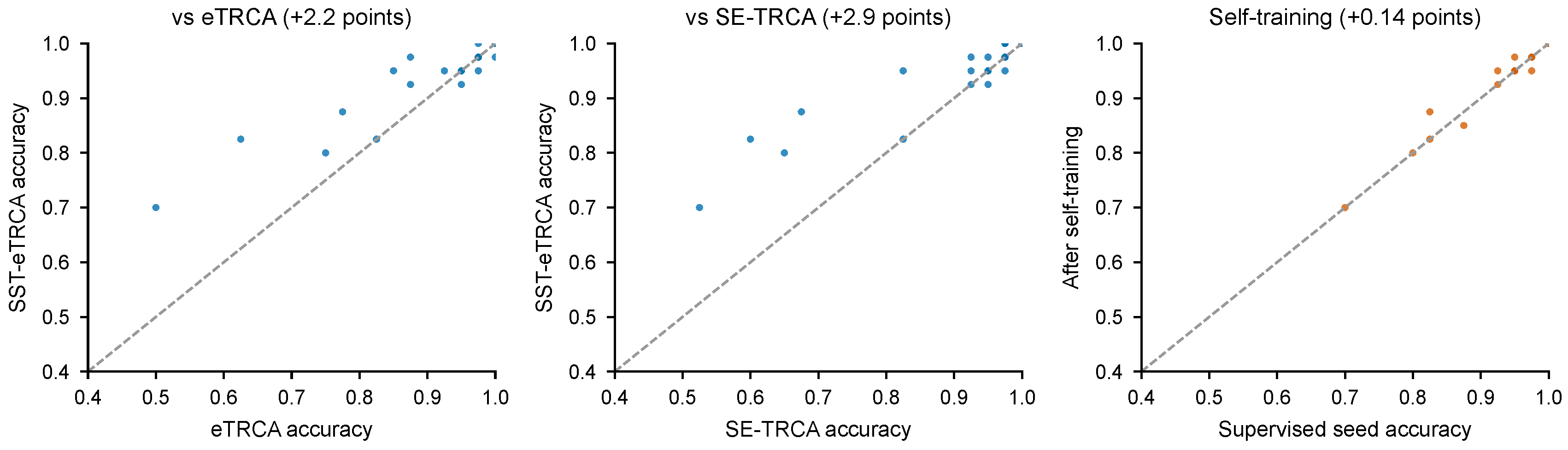
Figure 5.
Accuracy and ITR as a function of window length at one calibration trial per class. ITR is computed with the window length plus a 1 s inter-trial interval, so the curves cross where a shorter window buys speed at the cost of accuracy.
Figure 5.
Accuracy and ITR as a function of window length at one calibration trial per class. ITR is computed with the window length plus a 1 s inter-trial interval, so the curves cross where a shorter window buys speed at the cost of accuracy.
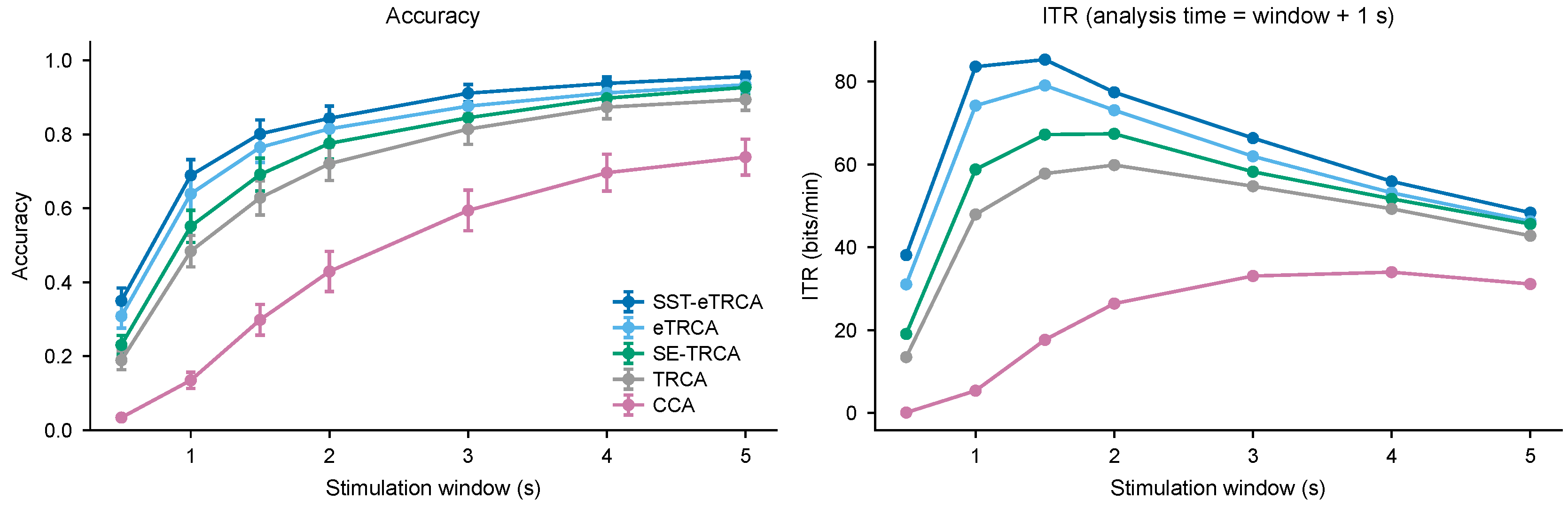
Figure 6.
Leave-one-subject-out accuracy for the five decoders, with and without one calibration trial per class from the held-out participant. The three TRCA variants are statistically indistinguishable; the gap to TRCA and CCA is preserved.
Figure 6.
Leave-one-subject-out accuracy for the five decoders, with and without one calibration trial per class from the held-out participant. The three TRCA variants are statistically indistinguishable; the gap to TRCA and CCA is preserved.
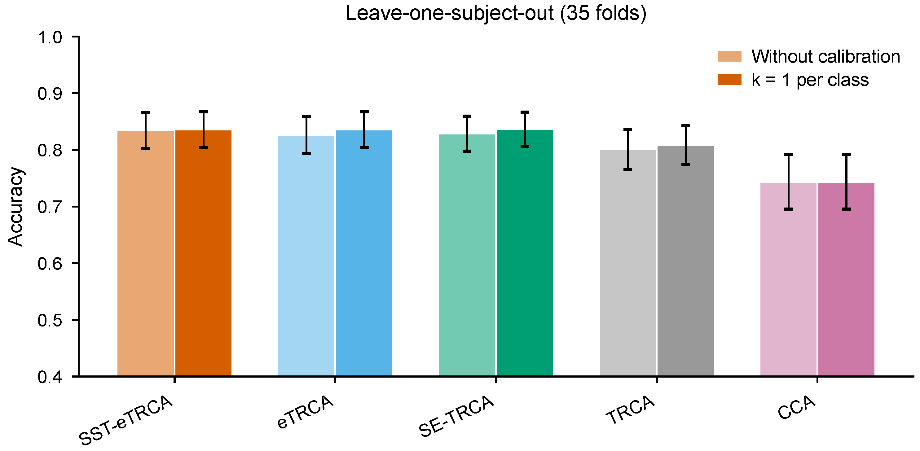

Table 1.
Stage-by-stage structure of the reader. Values are stored numbers; the projection and scoring stages hold no parameters. Shapes refer to n test trials, six channels and a 1247-sample augmented trial.
Table 1.
Stage-by-stage structure of the reader. Values are stored numbers; the projection and scoring stages hold no parameters. Shapes refer to n test trials, six channels and a 1247-sample augmented trial.
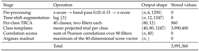 |
Table 2.
Held-out-block accuracy and ITR on the 35-subject benchmark (1400 decisions per cell). Brackets are 95 % Wilson intervals. ITR uses a 6 s analysis time. No self-training is applied in this table.
Table 2.
Held-out-block accuracy and ITR on the 35-subject benchmark (1400 decisions per cell). Brackets are 95 % Wilson intervals. ITR uses a 6 s analysis time. No self-training is applied in this table.
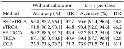 |
Table 3.
Paired comparisons against the proposed reader. b counts decisions where the reader is correct and the competitor wrong, c the reverse. Holm correction is applied within each budget condition over the four competitors. The upper block is without extra calibration, the lower block with one trial per class.
Table 3.
Paired comparisons against the proposed reader. b counts decisions where the reader is correct and the competitor wrong, c the reverse. Holm correction is applied within each budget condition over the four competitors. The upper block is without extra calibration, the lower block with one trial per class.
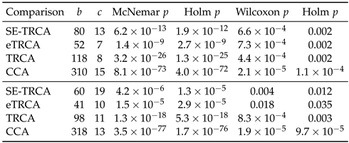 |
Table 4.
Effect of three rounds of transductive self-training. Columns give accuracy with the seed model and after self-training, and the difference in percentage points. CCA is excluded because the wrapper is not defined for a reference-based decoder.
Table 4.
Effect of three rounds of transductive self-training. Columns give accuracy with the seed model and after self-training, and the difference in percentage points. CCA is excluded because the wrapper is not defined for a reference-based decoder.
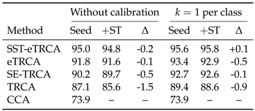 |
Table 5.
Accuracy (%) against stimulation window length at one calibration trial per class. The same held-out block is used at every length.
Table 5.
Accuracy (%) against stimulation window length at one calibration trial per class. The same held-out block is used at every length.
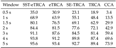 |
Table 6.
Leave-one-subject-out accuracy on the 35-subject benchmark (35 folds, 1400 decisions per cell). Values are mean ± standard deviation over participants. The source pool excludes the held-out participant in every fold.
Table 6.
Leave-one-subject-out accuracy on the 35-subject benchmark (35 folds, 1400 decisions per cell). Values are mean ± standard deviation over participants. The source pool excludes the held-out participant in every fold.
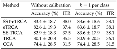 |
Table 7.
Ablation of the reader at one calibration trial per class. is the change in pooled accuracy relative to the full model, in percentage points. The McNemar test compares each variant with the full model on the same 1400 decisions.
Table 7.
Ablation of the reader at one calibration trial per class. is the change in pooled accuracy relative to the full model, in percentage points. The McNemar test compares each variant with the full model on the same 1400 decisions.
 |
Disclaimer/Publisher’s Note: The statements, opinions and data contained in all publications are solely those of the individual author(s) and contributor(s) and not of MDPI and/or the editor(s). MDPI and/or the editor(s) disclaim responsibility for any injury to people or property resulting from any ideas, methods, instructions or products referred to in the content. |
© 2026 by the authors. Licensee MDPI, Basel, Switzerland. This article is an open access article distributed under the terms and conditions of the Creative Commons Attribution (CC BY) license (http://creativecommons.org/licenses/by/4.0/).
Copyright: This open access article is published under a Creative Commons CC BY 4.0 license, which permit the free download, distribution, and reuse, provided that the author and preprint are cited in any reuse.