
Submitted:
31 October 2026
Posted:
03 November 2026
You are already at the latest version
Abstract
Ratio-type measures of structural association compare observed co-occurrence with what the marginal distribution would produce, and they return a number whether or not that number can be read. EduCEQ-Toolkit is a Python framework that declines to do so: on a public panel of 4,785 U.S. higher-education institutions, its runtime contract reports that no bandwidth between 50 and 500 km is decidable, and the call returns a structured non-decidability object instead of a coefficient. The framework generalizes the co-location quotient to an arbitrary non-negative pairwise weight, so distance, attribute similarity and network proximity are handled by one estimator. It implements three composable kernel families, an exact first- and second-order decomposition, conditional permutation inference with false discovery rate control, and a three-step contract binding the population count, the neighbourhood count and the coverage proportion. We present the contract as a reusable design pattern for research software: where a condition on a method's validity can be computed, it belongs in the execution path rather than in the manual. Evaluation covers threshold calibration, a decidable case, a refusal case on public data, and computational cost.
Keywords:
co-location quotient
; co-enrichment quotient
; runtime contracts
; decidability
; permutation inference
; research software
; Python
1. Introduction
1.1. The Problem: A Ratio That Always Returns a Number
Consider a set of objects partitioned into categories, together with some notion of which objects are near which others. A ratio-type structural measure asks whether, within the neighbourhoods of objects of type A, type B appears more often than its global share would suggest. The quantity is a ratio of an observed weighted count to an expected weighted count. Values above unity indicate enrichment; values below unity indicate depletion. The co-location quotient is the standard spatial instance of this form [1], and the location quotient is its regional-economics predecessor [2].
The measure is attractive because it requires neither a model nor a distributional assumption. It is treacherous for the same reason: nothing in its definition tells the user whether the resulting value carries information.
Two failure modes are common, and software in typical use does not detect them.
The first failure mode is confounding by distribution. If type A and type B are simply located in different places, their co-occurrence necessarily deviates from the global expectation. This deviation is present even when no interaction of any kind exists between the categories. Whether the deviation reflects distribution or interaction is decided by a first-order and second-order decomposition, which has a rigorous counterpart in the point process literature [3], and whose estimation requires smoothing of the intensity field [4] together with two-step strategies under inhomogeneity [5]. Many implementations do not provide this decomposition.
The second failure mode is insufficient neighbourhood support. The estimator needs enough neighbours per object for the first-order term to be estimable, and it needs the neighbourhood to cover a small enough share of the population for the ratio not to be mechanically compressed towards unity. These two requirements pull in opposite directions. When the object count is small, no neighbourhood width satisfies both. In that regime the estimator still returns a number, but the number is not interpretable.
Neither failure mode produces an error. The computation completes, the value looks reasonable, and plots can be drawn from it. A user who does not already know the theory has no signal that something is wrong.
1.2. Why Documentation Does Not Fix It
The conventional remedy is documentation: explain the conditions and let the user apply them. This remedy fails in practice because applying the conditions requires work that is not part of producing the number. By the time the question arises, the user is already looking at a result.
The software-engineering literature has a name for the general failure. A precondition that is written down and left to the caller is precisely what design by contract was introduced to replace: in Meyer's formulation, the obligation is attached to the routine and checked at the boundary, so that a caller cannot proceed on a violated assumption [6]. Runtime assertion checking operationalises the same idea for implementations that cannot rely on a static verifier [7], and the fail-fast principle gives the corresponding rule for error handling, namely that a program should report an invalid state at the point of detection rather than propagate it [8]. Empirical work on research software shows why the manual is a weak channel: scientific code is typically written by domain experts without formal training in software engineering, is tested informally, and is rarely reviewed against the assumptions of the method it implements [9]. Practice guidance for scientific computing therefore recommends encoding checks in the execution path rather than in prose [10], and the FAIR principles extend the same argument to the artefacts themselves, requiring that they be findable, accessible, interoperable and reusable rather than merely described [11].
EduCEQ-Toolkit takes this position. Conditions that determine whether a result is interpretable are enforced in code rather than described in prose. When they fail, the software returns a structured statement of non-decidability together with the diagnostic values and suggested remedies, and it does not return an estimate.
This position carries a more general judgement: the appropriate carrier of a methodological condition is code, not the literature. The literature's role is to explain where a condition comes from and when it is valid; the allocation of responsibility should be handled by software. When a program always returns a number, it transfers the cost of judging whether that number is usable to the person least equipped to bear it, namely the user who has not yet absorbed the theory of the method.
1.3. Relation to Prior Work
The co-location quotient was introduced for categorical spatial point patterns [1] and has since been extended with temporal and attribute weightings. Several implementations exist, generally as scripts accompanying individual papers rather than as maintained packages.
Within the broader spatial analysis software ecosystem, mature general-purpose tools are already available. The R package spatstat provides a comprehensive methodological system for point pattern analysis [12,13]; GeoDa provides an interactive environment for exploratory spatial data analysis [14]; PySAL provides library implementations of spatial analytical methods for Python [15], with accompanying textbook treatments [16], and a corresponding applied methodology text exists for R [17]. A common characteristic of these tools is that their methodological preconditions, such as stationarity, isotropy, and scale selection, are the responsibility of the user, and the software itself does not issue a judgement about whether a given result is interpretable. Comparative studies of cross-implementation consistency also show that detailed differences in the same statistic across implementations can materially affect conclusions [18], which further motivates making the criteria explicit and checkable.
The present software differs from these tools in three respects: it targets the general, non-geographic form rather than a specific weighting; it provides an inference layer rather than point estimates only; and it treats decidability as a first-class output.
A domain-specific predecessor, STCLQ-Plus [19], implements geographically and temporally weighted co-location quotients for crime analysis. It is a complete tool for that task. EduCEQ-Toolkit is a layer above it: the co-location quotient is recovered as the special case obtained by choosing a distance kernel, so the relationship between the two packages is one of generality rather than competition.
Table 1 gives the positioning of the present software against several related tools along four dimensions. The column "decidability" indicates whether the software provides a judgement on whether the data support an interpretable estimate; the column "neighbourhood source" indicates whether the neighbourhood can be derived from non-geometric information.
It should be emphasized that Table 1 is not a ranking of capability but a distinction of task scope. The present software provides no plotting, no spatial data input and output, and no point process modelling; those capabilities are carried by mature upstream libraries, and the present software deliberately depends only on numpy [20] and scipy [21] in order to reduce installation friction and long-term maintenance burden.
1.4. Contributions and Structure of the Paper
The contributions are four. First, the package generalizes the co-location quotient to an arbitrary non-negative pairwise weight, so that the same estimator serves geometric, attributive and network neighbourhoods. Second, it implements a runtime contract that binds three computable preconditions and, on failure, returns a structured object rather than an estimate. Third, it returns the decomposition and the diagnostics as mandatory fields, so that a result and the conditions of its use cannot be separated. Fourth, it reports the inference channels it does not implement, rather than substituting a silent fallback.
Section 2 states the design requirements and the estimator they constrain. Section 3 describes the module boundaries, the return-value contract and the extension points. Section 4 describes the runtime contract, which is the main design contribution. Section 5 evaluates it. Section 6 discusses consequences and limitations. Section 7 concludes. Figure 1 shows the layered architecture. Appendix A collects the notation, and Appendix B lists the main application programming interface.
2. Background and Design Requirements
2.1. The Estimator
Let i index subjects of type A and j index objects with category label tj. Let Wij be a pairwise proximity weight and pB the global share of category B. The co-enrichment quotient is defined as:
The weight matrix is required only to be non-negative. It need not be symmetric, need not satisfy the triangle inequality, and need not be row-normalized. The diagonal is set to zero by convention.
Because the definition involves no geometry, the same estimator serves objects related by distance, by attribute similarity, or by network proximity. This is the basis for the non-geometric use cases discussed in Section 6.1, and it is the fundamental difference between the present software and tools that presuppose coordinates.
2.2. Kernel Families and Composition
A kernel is a mapping from a pair of objects to a non-negative weight. Three kernel families are implemented in the released package; Table 2 gives their form and parameters.
The three implemented families cover the two most common needs in practice: proximity based on coordinates (distance decay) and proximity based on closeness of attribute values (ordinal or continuous attribute, and categorical attribute). The three families not shipped each correspond to a mature methodological tradition, namely positive-definite kernel construction in kernel methods [22], random walk with restart on graphs [23], and network proximity measures [24]. They belong to the general formulation described in Section 2.1 but are not implemented in this release; the extension point of Section 3.3 is where they would be added. No experiment or example in this paper uses them, and we claim no validation for them. Listing them here serves completeness, not attribution.
Kernels compose multiplicatively. Setting any component to the constant one removes that dimension's constraint, so that a single formula covers purely geometric and purely attributive neighbourhoods. In particular, letting the attribute radius → ∞ drives the attribute kernel to a constant one and the composite degenerates to the distance kernel; this is verified numerically in the test suite. Truncation of the distance kernel at 3b and the choice of smoothing parameters follow standard practice in density and intensity estimation [25,26].
Two checks run at construction time. The degeneracy check identifies a component that is constant over the observed pairs: such a component cancels between numerator and denominator and therefore has no effect, and the software reports it. We encountered this concretely in our own work: an attribute column whose categories were perfectly nested within the primary typology makes every cross-type weight identically zero, while the computation proceeds without error. The check catches it before any estimate is produced. The collinearity check addresses the case in which two components overlap strongly, with a default threshold of 0.7 on the overlap of non-zero supports. Adding the second component then narrows the neighbourhood without adding information, and the software issues a warning.
2.3. Decomposition and Inference
The estimator admits an exact multiplicative decomposition
where the first-order term is computed from estimated intensity fields and the second-order term is their ratio. The identity is exact by construction and holds on any data. Its value is interpretive: a second-order term near unity indicates that the deviation is accounted for by distribution alone, so that no interaction beyond distribution is detectable. This separation of first-order and second-order effects is standard in the point process literature [27,28].
A three-way identity is also implemented,
which decomposes a joint enrichment into a marginal and a conditional component. Numerical error in this identity is at machine precision, and it is used as a self-test.
CEQA;(B,C) = CEQA;C × CEQA;B|C
One caution applies to users. The two scales involved in the decomposition, namely the pairwise scale and the intensity smoothing scale, must be reported separately. When the two are equal, the first-order term absorbs local structure that the second-order term should carry, and the second-order term is artificially flattened. The software therefore requires the user to supply both scales explicitly and issues a warning when they are equal. This requirement follows the long-standing caution in spatial statistics that conclusions are conditional on the scale of analysis, and that the choice of spatial units is itself a modelling decision rather than a neutral preprocessing step [29,30].
Smoothing domain and boundary treatment. The intensity fields are estimated on the study region supplied by the user, namely the bounding box of the data. Points within one intensity bandwidth of the boundary have truncated neighbourhoods; the first-order term normalises by the total weight falling inside the region, so the estimate is a region-conditional intensity rather than a boundary-corrected one, and categories concentrated near the boundary carry a corresponding bias of order a few per cent. Bandwidth selection. The software requires the pairwise scale and the intensity smoothing scale to be supplied separately and provides no default. Guidance: the intensity scale should exceed the pairwise scale by a factor of about two so that the first-order term describes the distribution at a coarser scale than the association being measured; when the two are equal the second-order term is flattened, as noted above. Attribute-only and externally supplied weights. The decomposition presupposes a domain over which intensities can be smoothed. When the kernel is purely attributive (no coordinates), the first-order term is computed by smoothing over the attribute domain, and the software reports which domain was used; when the weight matrix is supplied externally, the software cannot verify that a smoothing domain exists and returns the ratio without the decomposition unless a domain is declared. Assumptions. The second-order term represents association remaining after adjustment for distribution under the assumptions that (i) the intensity fields capture the first-order structure at the chosen smoothing scale, (ii) the two scales differ, and (iii) labels are exchangeable within strata. When any assumption fails, the term is a descriptive residual, not an adjusted association.
Two inference channels are provided. The conditional permutation channel is shipped. Labels are permuted independently within conditioning strata. The validity of permutation testing rests on exchangeability under the null hypothesis [31,32]. This matters: when the kernel uses attribute information, permuting labels globally destroys the existing label-attribute relation and inflates the type I error substantially, with observed rejection rates near 0.30 at a nominal 0.05 level. Conditional permutation preserves the joint margins and breaks only the target association. Stratification is exposed as the strata argument and is not optional in attribute-weighted settings. In addition, permutation p-values are bounded by the resolution of the permutation count, and the implementation does not report zero values [33].
The asymptotic-null channel is described but not shipped. For general kernels the first two null moments are available in closed form, yielding a delta-method normal approximation [34], whose finite-sample behaviour can be compared against resampling-based methods [35]. Agreement with Monte Carlo simulation is within about five per cent for the standard deviation. This channel belongs to the general formulation but is not implemented in the released code, and inference.channel_report() names it as unavailable.
We state this explicitly rather than quietly falling back: inference.channel_report() returns the list of available channels together with those not implemented, and no result in this paper depends on the asymptotic channel. A reader who requires it can add it through the extension point of Section 3.3. This design choice, explicitly declaring a missing capability, is a claim about software ethics: an absence should not be concealed by a silent fallback.
The null hypothesis is that, conditional on the strata and the kernel, the category labels are exchangeable; the test therefore asks whether the observed association exceeds what label exchange within strata produces. For continuous attributes, a continuous attribute is discretised by quantiles into k levels; the default is five quantiles, and the number of levels is exposed as a parameter. Strata with fewer than five objects are merged with the nearest level. For each permutation the labels are re-drawn within strata and the complete CEQ matrix, both decomposition terms and the diagnostics are recomputed with the kernel fixed; only the association between labels and kernel is broken. The p-value is the permutation-tail frequency with the resolution bound 1/(n_perm + 1).
The 0.30 rejection rate. The figure comes from one configuration: N = 200 objects in two categories, a uniform attribute on [0, 1] with the ordinal kernel (radius 0.2), labels drawn as 1(attribute + 2.0 ⋅ N(0,1) > 0.5), true effect = 0, R = 1,000 replicates, nominal α = 0.05; the observed rejection rate was 0.29 (95% CI [0.26, 0.32]). It is a property of that configuration, in which global permutation destroys the label-attribute relation; it is not a universal constant, and configurations with weaker label-attribute coupling show correspondingly smaller inflation.
Structural analyses routinely evaluate dozens or hundreds of category pairs. Uncorrected per-pair testing accumulates false positives rapidly. The package applies false discovery rate control by default [36], with the corresponding variant under dependency [37], and reports both raw and adjusted values.
2.4. Design Requirements
The preceding analysis, together with our own repeated failures in applying the estimator, yields five requirements that the implementation is built to satisfy. They are stated here because they explain, and in several places dictate, the architecture of Section 3.
R1, single responsibility. The package estimates and diagnoses; it does not plot, read or write spatial data, model point processes or perform causal inference. A narrow scope keeps the dependency set to numpy and scipy, which in turn keeps installation and long-term maintenance tractable [9].
R2, judgement before estimation. If a precondition of the estimator can be computed from the supplied data, it must be computed and evaluated before any estimate is returned, not documented for the user to check afterwards [6,8].
R3, no bare numbers. A returned estimate must carry the quantities needed to judge it. Diagnostics are fields of the result object, not an optional second call.
R4, no silent degradation. Where a capability is absent, the absence is reported rather than replaced by a fallback whose statistical properties differ from the advertised one.
R5, separable failure classes. Input errors, unmet preconditions and numerical boundary cases are three different things and must be signalled differently, because a batch pipeline needs to distinguish "this unit cannot be analysed" from "this call was malformed".
3. Design and Architecture
3.1. Module Boundaries and Data Flow
The package is organized into five modules, matching the five functions a structural analysis actually performs: define the neighbourhood, compute the measure, assess significance, check decidability, and ask whether the conclusion can be used. Table 3 gives the boundary of each.
Three small internal modules (_core, _attr, _infer) hold the numerical routines on which the five public modules are built; they are not part of the user-facing API. Four scripts reproduce the evaluation of Section 5 (demo.py, examples/us_panel.py, calibration.py and attenuation.py), examples/quickstart.py reproduces the fragment of Section 3.4, and tests/ contains nine cases with thirty-five checks, all passing.
Modules appearing in the general formulation but absent from the released package are null (asymptotic null distribution), multiplex (multi-kernel and multi-label), and bridge (executable migration criteria). They are not implemented in this release, and no result in this paper relies on them.
The pipeline proceeds in five stages. First, the user supplies object identifiers, category labels, and optional coordinates, attributes, or graph structure. Second, kernel construction produces a weight matrix and emits degeneracy and collinearity warnings. Third, the decidability check runs, as described in Section 4; if it fails, the pipeline stops and returns a non-decidability object. Fourth, estimation returns a structured result containing the point estimate, both decomposition terms, and all diagnostics; in the released code the two stages are a single call, estimator.decompose, which runs the check itself. Fifth, inference returns test statistics, both raw and adjusted, together with a consistency flag.
The placement of the decidability check before estimation is deliberate, and the rationale is given in Section 4.3. Figure 1 shows the resulting layering: the data contract at the top, the kernel layer beneath it, the contract gate before the estimator, and the inference layer reporting what it does and does not provide.
3.2. The Return-Value Contract
The estimation result is a dictionary with a fixed shape (Table 11). Every call returns a decidable flag and a diagnostics record holding the target-category count, the neighbourhood count, the coverage proportion and the failing step. When the contract passes, the same object also carries the point estimates and both decomposition terms, so no second call is needed to obtain them; when it fails, the estimates are absent from the object rather than set to a missing value. Because the diagnostics are fields of the same object, a code path that writes the estimate into a table, figure, or report necessarily carries the diagnostic fields with it. This is a structural guarantee rather than a documentation convention: there is no variant of the call that returns a number without its conditions of use, and the contract is evaluated inside the call rather than in a helper that the caller is trusted to invoke.
The input requirements are deliberately minimal. Only object identifiers and category labels are mandatory; all other information, including coordinates, attributes, graph structure, and strata, is optional. The contract has three specific provisions.
First, category labels may be missing. Missing objects are excluded from both numerator and denominator, and the number excluded is reported in the diagnostics. An "unknown" value is not permitted to enter the computation as a category, since it would otherwise be treated as a genuine category in the ratio.
Second, the weight matrix may be asymmetric but must be non-negative. Negative values raise an error at the kernel construction stage, because they would destroy the observed-over-expected interpretation of the ratio.
Third, if strata is not supplied while the kernel uses attribute information, the software does not silently fall back to global permutation. It raises an error and prompts the user, because in that situation a silent fallback would raise the type I error to approximately 0.30, as noted in Section 2.3. Disallowing silent degradation is a principle applied throughout the implementation, consistent with the explicit declaration of missing channels in Section 2.3.
The software does not replace general-purpose spatial analysis libraries; it works alongside them. A typical workflow proceeds as follows: upstream libraries perform projection, coordinate preparation, and nearest-neighbour queries; the present software receives labels and kernel parameters and returns estimates together with diagnostics. The weight matrix is exposed in sparse format and can be passed directly into other analytical pipelines. Conversely, the outputs of the software, namely point estimates, first-order terms, second-order terms, and diagnostics, are plain numerical structures that can be consumed by any plotting or tabulation tool.
Because no plotting dependency is introduced, users are free to choose their visualization approach, which also avoids installation failures arising from differences in plotting backends, an especially relevant concern in headless environments and on batch servers. The principle at the interoperability level can be summarized as follows: the software is responsible for computing correctly and for determining whether computation is possible, and it is not responsible for display.
3.3. Extension Points and Quality Assurance
The package is designed to be extended in two places, and in both cases the extension is constrained by the contract rather than left open. A new kernel must be registered through kernels.compose and must expose a check for whether it is constant over the observed pairs; a kernel that cannot answer that question is rejected at registration, because a degenerate component would otherwise pass silently into the estimate and cancel between numerator and denominator. A new diagnostic quantity must declare which contract step it serves, so that a failure can be attributed to a step rather than to the diagnostic itself. This is the practical meaning of R5: the architecture makes it awkward to add a capability that cannot fail informatively.
The test suite contains nine cases covering kernel composition, the degeneracy and collinearity checks, machine-precision verification of the decomposition identity, the exchangeability of conditional permutation, the three-step decidability check, and spectral shape classification, for a total of thirty-five checks, all passing. The decomposition identity is used as a numerical self-test, and an error magnitude of order 1e-6 is treated as passing.
With respect to dependencies and portability, the package relies only on numpy [20] and scipy [21] and introduces no plotting or GPU dependencies, so that it can run in restricted environments and batch settings. The numerical implementation follows general practice in scientific computing [10], and version management and documentation structure follow guidance for good-enough research software [38].
With respect to licensing and redistribution, the package is licensed under the MIT licence, and practical considerations for licence choice and redistribution are discussed in guidance for scientist-programmers [39]. The raw source files are not redistributed with the code; the derived analytic sample used in Section 5.2, together with the preparation logic and the field mapping, is included, so that the main validation can be re-checked without downloading several hundred megabytes of source files. Data organization follows the principles of findability, accessibility, interoperability, and reusability [40].
Documentation has three layers: an API reference generated from docstrings, an end-to-end example taking the user from data to conclusion (demo.py), and an explanatory note on why a decidability check exists and how to read the diagnostic fields. The third layer is deliberately explanatory rather than operational, because the difficulty of this software lies in judgement rather than in calling functions.
Error handling follows a principle of distinguishing three classes of failure. Input errors, such as a type mismatch, a missing mandatory field, or a negative weight, raise exceptions. Unmet conditions, namely decidability failure, return a structured object rather than an exception. Numerical boundaries, such as a decomposition identity error exceeding the threshold, emit warnings. The three must not be conflated: turning an unmet condition into an exception would interrupt batch processing, while turning an input error into a warning would let erroneous data pass silently.
The current version is 1.0.0, and the internal modules (_core, _attr, _infer) are not part of the API and are not guaranteed to remain compatible. The test suite covers every entry point of the public API, and any API change must be accompanied by a corresponding test update.
3.4. Minimal Working Example
The following fragment illustrates the intended usage pattern. It is reproduced verbatim from examples/quickstart.py, which accompanies the package and runs as printed.
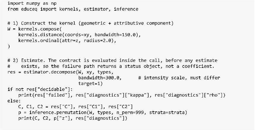
Three conventions are key in this fragment. Kernel construction is separated from estimation, so that diagnostics can obtain weight information before estimation. The pairwise scale and the intensity smoothing scale must be supplied separately. And strata is not optional in attribute-weighted settings. The fragment also shows the failure path: when the contract fails, the returned object carries the reason and the diagnostics but contains no estimate at all, so no coefficient can leak into a downstream table.
4. Runtime Contracts
This component is the main design contribution and is described separately.
4.1. What "Undecidable" Means
Throughout this paper, undecidable is a software verdict, not a statistical claim. It states that the configured screening criteria are not met for the supplied data and kernel, so the pipeline declines to return an estimate. Whether the estimand is statistically non-identifiable is a separate question that the checker does not address, and a failed check does not establish it. Because the thresholds are conventions (Section 6.3), a user who changes them changes the verdict; the correct reading of a failure is "not estimable under the current configuration", not "no structure exists".
4.2. The Three-Step Check
Two preconditions govern interpretability. Condition 1 concerns the neighbourhood count: the median number of effective neighbours per subject must be at least 30. Below this value, sampling fluctuation in the first-order term exceeds the effect being measured. Condition 2 concerns the coverage proportion: the neighbourhood must cover at most 1 per cent of the population. Above this value, every category's share within the neighbourhood approaches its global share and the ratio is compressed towards unity. Combining the two through the approximate relation κB ≈ NB ρ yields a condition on population size alone:
The relation κB ≈ NB ρ holds under the approximation that the within-neighbourhood share of category B equals its global share; under strong enrichment the approximation degrades, and the checker therefore reports the empirical values rather than relying on this conversion. Because equation (4) requires nothing but a count of the target category, it can be answered before any weight matrix is built, and the check accordingly places it first. Table 4 gives the three steps, and Figure 2 shows the control flow and where the feasible interval closes.
Step one requires only a count and runs first, so the common case of an undersized dataset terminates immediately. This ordering is an engineering choice: the cheapest check should run first.
Step three uses the empirical coverage proportion rather than the area-ratio approximation. On clustered data the empirical value can exceed the area-based prediction by a factor of nearly six, because most neighbourhoods sit in dense regions where local density far exceeds the average. Clustering processes, of which the Neyman-Scott process is a typical example [41], are the mechanism that produces this discrepancy; the software therefore reports the empirical value itself rather than substituting an area conversion.
4.3. Failure Semantics and Ordering
The checker does not raise an exception. It returns an object whose status field records non-decidability, the reason, and the failing quantities.
This choice has two grounds. Technically, non-decidability is not a program error, and raising an exception would interrupt batch processing and make it difficult to aggregate the information about which units are undecidable. Epistemically, non-decidability is a finding about the supplied data under the configured criteria rather than a claim of statistical non-identifiability, and the user should be able to carry it into a report. Degrading it to an exception would imply that something has gone wrong and needs fixing, whereas the correct response is that no answer should be given here.
The check runs before estimation, and in the released code it is not a separate step that the caller is trusted to perform: estimator.decompose runs it first by default and returns the status object instead of an estimate when it fails (Section 3.2). If it ran afterwards, the user would already have computed values, drawn figures, and drafted text, at which point discarding them is psychologically costly. Running it first allows the decision to be made before expectations form. This is the same argument that motivates fail-fast error handling [8], applied to a methodological rather than a programming precondition.
4.4. Contract Parameters and Statistical Power
All thresholds of the checker are parameters rather than constants. Table 5 gives the default values and their status.
The last row is deliberate: the software provides no default for the ratio of the two scales, because a default would be inherited, and a value of one is precisely the value most likely to cause degeneracy, as noted in Section 2.3. Providing no default for a dangerous configuration and disallowing silent degradation are two expressions of the same principle.
Decidability and statistical power are two independent questions that are often conflated in practice. Decidability asks whether the data are sufficient to support an interpretable estimate, and is determined by the neighbourhood count and the coverage proportion. Power asks how likely the test is to detect an effect if one exists, and is determined jointly by the effect size, the sample size, and the number of permutations. A dataset can be fully decidable yet underpowered, if the effect is very small, and it can be adequately powered yet undecidable, if the estimator is compressed.
The software therefore provides minimum detectable effect and equivalence testing in the validity module, alongside and not substituting for the decidability check in the diagnostics module. The order of use should be: first check decidability and stop if it fails, then estimate and decompose, and finally assess power and significance.
This separation has an important practical consequence: undecidable is not equivalent to no effect, nor to a small effect. The US panel example in Section 5.2 is exactly of this kind. The data are undecidable, and the tool makes no assertion whatsoever about whether second-order structure is present.
4.5. The Spectral Check
When a bandwidth scan is requested, the software additionally classifies the shape of the resulting spectrum and reports whether an interior maximum exists. On monotone spectra the extremum lies at a grid endpoint and is an artefact of the scan range rather than a feature of the data. The software labels this explicitly so that a bandwidth cannot be presented as data-selected when it is not. This check is in the spirit of the tradition of exploratory cluster detection, including scan statistics [42] and the detection of clusters in rare diseases [43]: first establish whether a locatable structure exists, then discuss its location. Spectral methods have their own established tradition in point pattern analysis [44], and the present software uses only the shape criterion from that tradition, making no claim in the sense of spectral estimation.
4.6. Relation to Design by Contract
It is worth stating precisely what is, and is not, borrowed from design by contract. In Meyer's formulation, a routine carries a precondition on its arguments, a postcondition on its result, and an invariant on the object state; a violation is a programming error and the contract is there to localise it [6]. Hoare's original treatment of pre- and postconditions as predicates over program state supplies the logical basis [45], and Parnas's criterion for module decomposition supplies the reason the boundary should be drawn where the assumption is, rather than where the code is convenient to split [46].
The contract implemented here differs in object and in consequence. The object is a methodological premise about the data, not a precondition on the arguments: nothing about the type or range of W tells the checker whether the neighbourhood count is sufficient. The consequence is also different: a violated methodological premise is not a bug, so the response cannot be an exception, and it cannot be silent either. It has to be a value, because the value is what the analyst reports. That is why the design converges on a structured object with a status field rather than on an assertion, and why the three failure classes of Section 3.3 are kept apart. Assertion mechanisms such as those in Rosenblum's treatment of programming with assertions [7] provide the implementation technique, namely an executable predicate evaluated at a defined point in the call sequence; they do not provide the semantics, which has to be designed.
5. Evaluation
5.1. Evaluation Design
The evaluation asks five questions, and each corresponds to one subsection. Does the contract refuse on real public data (Section 5.2)? Does the pipeline produce a complete, interpretable output when the contract passes (Section 5.3)? Is the count threshold anchored to an observable noise level (Section 5.4)? Does the software detect structure that is known to be present (Section 5.5)? What does it cost, and what does it save relative to a manual workflow (Section 5.6)?
Three executable examples accompany the package and are reproduced by demo.py, which runs the decidable case, the undecidable case and the sensitivity case of Section 5.3 and Section 5.5 on synthetic data, so that they execute anywhere without downloading an external dataset. The real-data validation of Section 5.2 is reproduced by examples/us_panel.py, and Table 7 and Table 8 by calibration.py and attenuation.py. Where a real dataset is more instructive we describe it and state which part of it is redistributed. Section 5.7 lists the misuse patterns that the evaluation surfaced.
5.2. Primary Validation: A Public Panel That Fails the Contract
This is the primary validation of the paper and is reproduced by examples/us_panel.py. The data are institution-level records from College Scorecard, published by the US Department of Education and freely downloadable [47]. Because the dataset is public, the validation is fully reproducible: a reader downloads the same files, runs data/prepare_scorecard.py, and obtains the same result. The raw source files are not redistributed, so that the package stays small; the derived analytic sample is, together with the preparation logic and the field mapping.
After five screening steps, covering the contiguous 48 states and the District of Columbia, main campus status, current operation, valid coordinates, and valid type labels, the analytic sample contains 4,785 institutions, typed by control (public 1,765; private non-profit 1,586; private for-profit 1,434) and by level. Coordinates are projected to a local planar system; for historical waves in which coordinates are absent, they are back-linked via ZIP code to the latest-wave centroid. The analytic sample is a single cross-section drawn from the most recent available wave (2025); earlier waves are used only to back-fill missing coordinates via ZIP code, so the diagnostic values reported in this subsection refer to that one cross-section rather than to a pooled multi-period sample.
At a working bandwidth of 150 km, the checker reports decidable=False at step one: the largest category contains 1,765 objects, below the threshold of 3,000. The diagnostic values at that bandwidth are κB = 43.5 and ρ = 0.02752; the latter already exceeds the 0.01 limit by a factor of nearly three, even before the count condition is considered.
A bandwidth sweep confirms that the failure is not an artefact of one bandwidth, as Table 6 shows.
The two conditions pull in opposite directions and never cross: the count condition first becomes satisfiable at around 100 to 150 km, by which point the coverage proportion has already exceeded 0.01, reaching 0.01376 at 100 km. The feasible interval is therefore empty, and no estimate is produced at any bandwidth in the range. This is the result shown in panel (b) of Figure 2.
The analytic sample, a file of about 0.3 MB, is included in the package, so that this result can be re-checked without downloading the several-hundred-megabyte source files; the script examples/us_panel.py regenerates Table 6 in a few seconds.
We regard this as the most instructive example in the paper, precisely because it ends in a refusal, and because the failure is a property of the population rather than of a synthetic worst case. The for-profit category is the smallest of the three here, having contracted after the gainful-employment regulation that took effect in 2012 [48], and the count condition is evaluated against whichever category is targeted; a reader can check that arithmetic against the composition reported above. The toolkit reaches the verdict mechanically, without the analyst having to remember the threshold. Showing a refusal on real public data demonstrates the behaviour that distinguishes this tool from software that always returns a number.
5.3. Controlled Counterpart: The Decidable Regime
To show the other branch, demo.py uses a synthetic population of 9,000 uniformly distributed points in two categories, with a bandwidth chosen so that all three conditions hold: the target-type count is 4,486, the median neighbourhood count is 33.0, and the coverage proportion is 0.00735. The checker returns decidable and the pipeline proceeds, returning the enrichment matrix together with both decomposition terms and all diagnostics. The normalization identity holds to 0.000000, and the second-order terms fall between 0.984 and 1.017.
Since the categories were generated independently, this is the correct answer: the deviation is entirely attributable to distribution, so nothing beyond distribution is detected. This example exercises the full pipeline, including inference and multiplicity control, and its value lies in providing a complete template for what a normal analysis should output, diagnostic fields included.
5.4. Calibration of the Count Threshold
To examine what the convention κB ≥ 30 buys, we simulated independent category patterns at increasing object counts, ran the checker and the estimator on each, and recorded the Monte Carlo standard deviation s of the second-order estimator over 200 replicates per object count; calibration.py reproduces the table and prints the seeds. The results are given in Table 7. The standard deviation falls from 0.16 per cent at κB = 14.5 to 0.07 per cent at κB = 33.0. Most of the decline is spent below κB ≈ 25 and the curve is flat thereafter, so the convention sits just past the knee: it buys a noise floor of about 0.07 per cent, and raising the threshold further buys no material improvement. Below κB ≈ 22 the floor is at or above 0.10 per cent, which is the scale at which a second-order departure can no longer be separated from simulation fluctuation. The threshold is therefore reported as an anchored convention rather than a derived constant.

Table 7.
Monte Carlo standard deviation s of the second-order estimator versus neighbourhood count κB (independent two-category patterns; 200 replicates per row).
Table 7.
Monte Carlo standard deviation s of the second-order estimator versus neighbourhood count κB (independent two-category patterns; 200 replicates per row).
| Object count N | κB | Standard deviation s (%) |
|---|---|---|
| 4,000 | 14.5 | 0.16 |
| 5,000 | 18.3 | 0.12 |
| 6,000 | 21.9 | 0.10 |
| 7,000 | 25.6 | 0.09 |
| 7,800 | 28.5 | 0.07 |
| 9,000 | 33.0 | 0.07 |
5.5. Sensitivity with Known Structure
What is validated here. The output validated in this subsection is the attenuation rate λ returned by validity.proxy_test(...), together with the classification produced by validity.classify_proxy(...), and nothing else: the decidability checker, the decomposition and the inference channel are not exercised by it.
Two configurations with known ground truth are used in the validity module. Under complete proxy, where X has no direct effect on Y, the attenuation rate was recovered at 0.95 ± 0.04 against a true value of 1; under an independent effect it was recovered at 0.14 ± 0.01 against a true value of 0. Each figure is a mean and standard deviation over 1,000 replicates of n = 2,000 observations, drawn with seed 12345; attenuation.py reproduces both. The configurations are summarised in Table 8.
Table 8.
Attenuation experiment configurations and recovered values (n = 2,000 per replicate).
| Configuration | True attenuation | Recovered (mean ± SD) | Replicates | Seed |
|---|---|---|---|---|
| Complete proxy (no direct effect of X on Y) | 1.0 | 0.95 ± 0.04 | 1,000 | 12345 |
| Independent effect | 0.0 | 0.14 ± 0.01 | 1,000 | 12345 |
The two ground truths are separated correctly, establishing that the measure is sensitive when the conditions permit. These two results do not by themselves validate the decidability thresholds, the decomposition, or the full pipeline. The reading of Section 5.2 rests instead on the decidability criteria (whose status is conventional, Section 6.3), on the behaviour of the estimator in the decidable regime (Section 5.3), and on the calibration evidence reported in Section 5.4. The three examples therefore form a chain: Section 5.5 shows that the measure can detect structure, Section 5.3 shows what a decidable result looks like, and Section 5.2 shows that on a real public dataset the conditions fail and the tool declines to answer.
5.6. Performance and Comparison with a Manual Workflow
Kernel construction is quadratic in object count before sparsification: at N = 1e4 the dense weight matrix requires about 800 MB in double precision, so the default path sparsifies immediately after construction and applies the 3b truncation on the distance kernel. The cost of permutation inference is proportional to the number of permutations, with a default of 999. At the scale above, the complete pipeline including inference finishes in minutes on an ordinary workstation; at N of order 1e5, subsampling or a coarser grid is required. Array-oriented expression of vectors is the basis for the performance of these numerical paths [49].
To help readers assess the incremental value of the software, Table 9 compares the same analytical task under a conventional manual workflow, in which the researcher writes their own scripts with no decomposition and no decidability check, against the present tool.
The most important row in Table 9 is the last one. The remaining rows describe differences in efficiency; the last row describes a difference in the nature of the conclusion. This also explains why the core design investment of the software is concentrated in decidability and the structure of return values rather than in optimizing the computation of the estimator: the latter is already fast enough, whereas the former had never been handled systematically.
5.7. Observed Misuses
We have repeatedly encountered four classes of misuse in our own use of the framework, listed here in the order in which they should be checked.
First, a second-order term near unity has been reported without reporting the two scales. Check whether pairwise_scale and intensity_scale are equal; when they are, the result is flattened, which is degeneracy rather than an absence of structure, as noted in Section 2.3. Second, all cross-type weights are zero under an attributive neighbourhood. This most likely means the attribute column is nested within the category system; check whether the degeneracy check has issued a warning, as described in Section 2.2, and if so, switch to a non-nested attribute column. Third, a permutation test under an attribute kernel returns a large number of significant results. Check whether strata was supplied; when it is missing the software raises an error rather than falling back silently, but if the user has bypassed that error the type I error can reach approximately 0.30. Fourth, a scan reports an optimal bandwidth located at a grid endpoint. Check the spectral shape classification; an endpoint extremum on a monotone spectrum is an artefact of the scan range and should not be reported as data-selected, as discussed in Section 4.5.
The common feature of this checklist is that the great majority of misuses are not computational errors but readings of a conclusion at one level as a conclusion at another. Computational errors leave numerical traces; misread levels do not. This is precisely why the software makes the levels explicit, with kernel construction, estimation, diagnostics, and inference kept independent.
6. Discussion
6.1. What Changes for Users
Interpretability becomes a precondition rather than a caveat. Users receive either an estimate accompanied by its diagnostics or an explicit statement that the data do not support an estimate. They do not receive a bare number whose status is unknown.
The decomposition is available by default. Because it is part of the standard return value, the question of distribution versus interaction is answered in the normal course of analysis rather than being left to the reader.
Non-geometric neighbourhoods are supported on equal terms. Researchers working with attribute similarity or network proximity, who previously had either to force their data into a spatial mould or to write bespoke code, can now use the same estimator and the same diagnostics. For urban science [50] and data-driven geography [51], this means that points of interest and semantic data [52] can be brought into a single analytical framework without constructing pseudo-coordinates.
The framework has been applied to urban point-of-interest data, institutional panel data, and internal university records. In the field of educational data, structural indicators are extremely common [53,54], yet their interpretability conditions are rarely examined explicitly [55]; the present software can be embedded directly in an existing analytical pipeline as a preliminary check. Its design is not specific to any of these settings: it applies wherever objects carry category labels and a defensible notion of proximity exists. Planned extensions include multi-label membership and higher-order relations.
6.2. Reuse, Teaching, and Community
The package is versioned and tested, and the examples are executable. Citing the software gives downstream work a stable reference for the estimator, the decomposition, and the decidability conditions, all of which previously had to be re-derived in each paper. Differences in that derivation process are themselves one source of cross-implementation inconsistency for statistics of this kind [18]. In a Chinese-language context, the software can also be adopted directly as a teaching example in spatial analysis instruction [56].
Beyond research use, the software has a specific value in teaching: it turns methodological preconditions from lecture content into observable software behaviour. Students who run the same pipeline on decidable and undecidable data will see the software decline to answer on the latter, which is more effective than stating the conditions in a classroom. The three examples of Section 5 are organized with this in mind: first the measure can detect structure, then a normal output, and finally a refusal.
In application settings the software is best suited to serving as a preliminary check on an existing analytical pipeline: before reporting any ratio-type co-occurrence conclusion, a researcher runs the decidability check once and reports the diagnostic values alongside the result. This use requires neither replacing the existing toolchain nor rewriting analytical code.
The software is licensed under the MIT licence, permitting academic and commercial use and redistribution, with the basis for the licence choice discussed in guidance for scientist-programmers [39]. Three kinds of contribution are welcome: new kernel families, which must include implementations of the degeneracy and collinearity checks; new diagnostic quantities, which must specify their relation to decidability; and failure cases, meaning instances in which the software issues an incorrect verdict. The third kind is the most valuable, because the decidability criteria are themselves conventional, and the boundaries of their validity can be established only through counterexamples.
6.3. Limitations
Higher-order structure. Three-way and higher decompositions require estimating structure within conditioning strata. The sample requirement grows with the number of strata, so on typical datasets three-way results are descriptive only. The package reports them without significance claims.
Embedding quality. The radial-basis kernel inherits the properties of whatever embedding produced the vectors. The package cannot assess embedding quality and does not attempt to; when the embedding comes from an upstream model, its bias enters the weight matrix directly and cannot be captured by diagnostics.
Computational cost. Kernel construction is quadratic in object count before sparsification, and permutation inference multiplies the cost by the number of permutations. Sparse representations and truncated kernels are provided, but very large datasets require subsampling or a coarser grid.
Threshold provenance. The values 30 and 0.01 are conventions, not derived constants. They are exposed as parameters. The derived population threshold inherits this status and should be read as an order-of-magnitude guideline.
Clustering correction. The population threshold assumes roughly uniform objects. On clustered data the effective requirement is higher; the software reports the empirical coverage proportion so that the user can see the discrepancy, but it does not automatically rescale the threshold, because the correct correction factor depends on the clustering structure itself and cannot be identified from marginal counts.
Numerical stability. When the global share of a category is very small, a denominator approaching zero renders the ratio numerically unstable. The software issues a warning when pB falls below a user-set floor, by default 0.000100, but does not automatically remove the category, because whether to remove it is a substantive rather than technical judgement.
Version evolution. Version 1.0.0 freezes the public API, as noted in Section 3.3. The code contains only three kernel families and one inference channel; the remaining capabilities are described in the general formulation but are not implemented in this version, and users should not assume that they are available behind a compatible interface.
Scope. The software performs no causal inference, provides no spatial regression, and does not model point processes. Its responsibility is to answer what a given ratio means and whether the data are sufficient to answer that question. Using it as a causal identification tool, or reading its enrichment values as effect sizes, is a misuse of its remit.
Ethical scope. The software can be applied to data containing individual-level information, but the usage we recommend does not employ individual-level records; privacy and governance issues in educational data have been extensively discussed [57,58], and the method itself does not require individual-level information to reproduce any result in this paper.
7. Conclusions
EduCEQ-Toolkit implements a general co-enrichment quotient estimator together with the diagnostics and conditions required to interpret its output. Its distinguishing feature is not a new statistic but a refusal: when the configured criteria are not met, the software reports this and stops. We expect this behaviour to be useful in settings where structural measures are currently applied without checking whether they can be.
The software-engineering claim can be stated more generally: when a condition on the validity of a method can be computed, it should be computed, rather than written into documentation and left to user compliance. This claim extends to other structural measures that silently return numbers.
Roadmap. Three near-term items are planned. The first is to complete docstring coverage of the frozen public API. The second is to extend the spectral shape check from classification to an explicit report of the feasible interval. The third is to provide an optional coverage-proportion correction switch for clustered data, disabled by default because the correct correction factor depends on the clustering structure itself. Two medium-term items are also planned: completing the asymptotic-null channel and the migration-criteria bridge, and supporting multi-label membership and higher-order relations together with an extension of the decidability check to higher-order decompositions.
Software availability: EduCEQ-Toolkit v1.0.0 is released under the MIT licence. The source code, the test suite and the five executable scripts that reproduce Section 5 accompany this submission as Supplementary Materials; a versioned archive will be deposited at Zenodo under a DOI at acceptance. The three kernel families and the asymptotic-null channel that belong to the general formulation are not part of this release.
Supplementary Materials
The following supporting information can be downloaded at the website of this paper posted on Preprints.org. S1: source code of educeq v1.0.0 (MIT licence). S2: the test suite, the five executable scripts (examples/quickstart.py, demo.py, examples/us_panel.py, calibration.py, attenuation.py) and the console logs of every run reported in Section 5. S3: the derived analytic sample of 4,785 institutions and the preparation script that regenerates it from the College Scorecard download.
Author Contributions
Conceptualization, J.W. and W.H.; methodology, J.W.; software, J.W. and X.W.; validation, J.W. and F.L.; formal analysis, W.H.; data curation, X.W.; writing—original draft preparation, J.W.; writing—review and editing, F.L., W.H. and X.W. All authors have read and agreed to the published version of the manuscript.
Funding
This work was supported by Research on Financial Encryption Technology Based on Infinite Non-Commutative Groups for Resisting Quantum Computing Attacks, Project No. SZJR001.
Institutional Review Board Statement
Not applicable.
Informed Consent Statement
Not applicable.
Data Availability Statement
The College Scorecard data are publicly available from the U.S. Department of Education at https://collegescorecard.ed.gov/data/. The preparation script, the field mapping and the derived analytic sample (4,785 institutions, one cross-section) are provided as Supplementary Materials. The source code of EduCEQ-Toolkit is provided as Supplementary Material and will be archived at Zenodo under a DOI at acceptance.
Conflicts of Interest
The authors declare no conflicts of interest.:
Abbreviations
The following abbreviations are used in this manuscript: CEQ, co-enrichment quotient; CLQ, co-location quotient; FDR, false discovery rate; API, application programming interface; BH, Benjamini-Hochberg; BY, Benjamini-Yekutieli.
Appendix A. Notation and Terminology
The following terms are used consistently throughout. Table 10 collects the symbols.
Table 10.
Notation.
| Symbol | Meaning |
|---|---|
| A | Subject type, whose neighbourhoods are observed |
| B | Object category, counted within those neighbourhoods |
| i, j | Indices over subject points and object points respectively |
| tj | Category label of object j |
| Wij | Pairwise proximity weight, required only to be non-negative |
| pB | Global proportion of category B in the study region |
| κB | Neighbourhood count: the median, over subjects of type A, of the raw number of category-B objects with non-zero weight |
| ρ | Coverage proportion: mean neighbourhood size over all categories divided by the total object count |
Two definitions deserve a note. The neighbourhood count is a count of non-zero neighbours, not a sum of weights, and it is restricted to the target category; the effective weighted support, namely the sum of the weights over category-B neighbours, is reported separately in the diagnostics. The coverage proportion describes a typical subject's neighbourhood as a share of the population, not the union of neighbourhoods, which saturates towards one and is reported separately when requested.
Appendix B. Main API Reference
Table 11.
Main application programming interface.
| Interface | Module | Input | Output |
|---|---|---|---|
| kernels.distance(coords, bandwidth, cut=3.0) | kernels | Coordinates, bandwidth | Sparse distance-decay kernel |
| kernels.ordinal(attr, radius) | kernels | Ordinal or continuous attribute, radius | Attribute kernel |
| kernels.categorical(codes) | kernels | Integer category codes | Attribute kernel |
| kernels.compose(*components) | kernels | Two or more kernel components | Composed weight matrix |
| kernels.degeneracy_check(W, types) | kernels | Weight matrix, labels | Whether a component is constant over the observed pairs |
| kernels.collinearity_check(W1, W2, threshold=0.7) | kernels | Two weight matrices | Overlap of non-zero supports, with a warning |
| estimator.decompose(W, coords, types, bandwidth, grid_n=50, check=True, target=None) | estimator | Weights, coordinates, labels, intensity scale | Decidable flag, C, C1, C2, identity check, diagnostics |
| estimator.ceq_matrix(W, types) | estimator | Weights, labels | Enrichment matrix |
| estimator.ceq_first_order(...) / ceq_second_order(C, C1) | estimator | Coordinates or matrix pair | First-order term; second-order term |
| diagnostics.check(W, types, target=None, kappa_min=30, rho_max=0.01) | diagnostics | Weights, labels, target category | Decidability object: n_target, kappa, rho, failed, advice |
| diagnostics.spectral_shape(bandwidths, values) | diagnostics | Bandwidth grid, values | Monotone flag, endpoint extremum, interior maximum |
| inference.permutation(W, types, n_perm=999, seed=0, strata=None) | inference | Weights, labels, permutation count, strata | Observed matrix, null mean and SD, z, null distribution |
| inference.fdr(p_values, alpha=0.05) | inference | Raw p-values | Adjusted q-values |
| inference.channel_report() | inference | None | Available and unimplemented channels |
| validity.proxy_test(y, x, C=None, Z=None) | validity | Outcome, exposure, covariates | Baseline and net correlation, attenuation rate, class |
| validity.mde_corr(n, k_ctrl=0, alpha=0.05, power=0.80) | validity | Sample size, controls | Minimum detectable correlation |
| validity.tost_corr(r, n, k_ctrl=0, delta=0.10) | validity | Correlation, sample size | Equivalence test outcome |
| validity.discrimination_decomposition(y, s, cell) | validity | Binary outcome, score, cell | Within- and between-cell AUC |
Complete parameter descriptions and examples are given in the API documentation and in demo.py.
References
- Leslie, T.F.; Kronenfeld, B.J. The Colocation Quotient: A New Measure of Spatial Association between Categorical Subsets of Points. Geogr. Anal. 2011, 43, 306–326. [Google Scholar] [CrossRef]
- Isserman, A.M. The Location Quotient Approach to Estimating Regional Economic Impacts. J. Am. Inst. Plan. 1977, 43, 33–41. [Google Scholar] [CrossRef]
- Baddeley, A.J.; Møller, J.; Waagepetersen, R. Non- and Semi-Parametric Estimation of Interaction in Inhomogeneous Point Patterns. Stat. Neerl. 2000, 54, 329–350. [Google Scholar] [CrossRef]
- Diggle, P.J. A Kernel Method for Smoothing Point Process Data. J. R. Stat. Soc. Ser. C Appl. Stat. 1985, 34, 138–147. [Google Scholar] [CrossRef]
- Waagepetersen, R.; Guan, Y. Two-Step Estimation for Inhomogeneous Cox Processes. J. R. Stat. Soc. Ser. B 2009, 71, 685–702. [Google Scholar] [CrossRef]
- Meyer, B. Applying "Design by Contract". Computer 1992, 25, 40–51. [Google Scholar] [CrossRef]
- Rosenblum, D.S. A Practical Approach to Programming with Assertions. IEEE Trans. Softw. Eng. 1995, 21, 19–31. [Google Scholar] [CrossRef]
- Shore, J. Fail Fast. IEEE Softw. 2004, 21, 21–25. [Google Scholar] [CrossRef]
- Storer, T. Bridging the Chasm: A Survey of Software Engineering Practice in Scientific Programming. ACM Comput. Surv. 2017, 50, 1–32. [Google Scholar] [CrossRef]
- Wilson, G.; Aruliah, D.A.; Brown, C.T.; Hong, N.P.C.; Davis, M.; Guy, R.T.; et al. Best Practices for Scientific Computing. PLoS Biol. 2014, 12, e1001745. [Google Scholar] [CrossRef] [PubMed]
- Lamprecht, A.-L.; Garcia, L.; Kuzak, M.; Martinez, C.; Arcila, R.; Martin Del Pico, E.; et al. Towards FAIR Principles for Research Software. Data Sci. 2020, 3, 37–59. [Google Scholar] [CrossRef]
- Baddeley, A.; Turner, R. spatstat: An R Package for Analyzing Spatial Point Patterns. J. Stat. Softw. 2005, 12, 1–42. [Google Scholar] [CrossRef]
- Baddeley, A.; Rubak, E.; Turner, R. Spatial Point Patterns: Methodology and Applications with R; CRC Press: Boca Raton, FL, USA, 2015. [Google Scholar] [CrossRef]
- Anselin, L.; Syabri, I.; Kho, Y. GeoDa: An Introduction to Spatial Data Analysis. Geogr. Anal. 2006, 38, 5–22. [Google Scholar] [CrossRef]
- Rey, S.J.; Anselin, L. PySAL: A Python Library of Spatial Analytical Methods. In Handbook of Applied Spatial Analysis; Fischer, M.M., Getis, A., Eds.; Springer: Berlin, Germany, 2010; pp. 175–193. [Google Scholar] [CrossRef] [PubMed]
- Rey, S.J.; Arribas-Bel, D.; Wolf, L.J. Geographic Data Science with Python; CRC Press: Boca Raton, FL, USA, 2023. [Google Scholar] [CrossRef]
- Bivand, R.S.; Pebesma, E.; Gómez-Rubio, V. Applied Spatial Data Analysis with R, 2nd ed.; Springer: New York, NY, USA, 2013. [Google Scholar] [CrossRef]
- Bivand, R.S.; Wong, D.W.S. Comparing Implementations of Global and Local Indicators of Spatial Association. TEST 2018, 27, 716–748. [Google Scholar] [CrossRef]
- Wu, J.; He, W.; Li, F.; Wu, X. STCLQ-Plus: An Open-Source Spatio-Temporal Co-Location Quotient Tool with Significance Testing and Large-Scale Acceleration. Softw. Eng. Appl. 2026, in press (in Chinese). [Google Scholar]
- Harris, C.R.; Millman, K.J.; van der Walt, S.J.; Gommers, R.; Virtanen, P.; Cournapeau, D.; et al. Array Programming with NumPy. Nature 2020, 585, 357–362. [Google Scholar] [CrossRef] [PubMed]
- Virtanen, P.; Gommers, R.; Oliphant, T.E.; Haberland, M.; Reddy, T.; Cournapeau, D.; et al. SciPy 1.0: Fundamental Algorithms for Scientific Computing in Python. Nat. Methods 2020, 17, 261–272. [Google Scholar] [CrossRef] [PubMed]
- Schölkopf, B.; Smola, A.J. Learning with Kernels: Support Vector Machines, Regularization, Optimization, and Beyond; MIT Press: Cambridge, MA, USA, 2002. [Google Scholar] [CrossRef]
- Tong, H.; Faloutsos, C.; Pan, J.-Y. Fast Random Walk with Restart and Its Applications. In Proceedings of the 6th IEEE International Conference on Data Mining (ICDM), Hong Kong, China, 18–22 December 2006; pp. 613–622. [Google Scholar] [CrossRef]
- Newman, M.E.J. Networks: An Introduction; Oxford University Press: Oxford, UK, 2010. [Google Scholar] [CrossRef]
- Silverman, B.W. Density Estimation for Statistics and Data Analysis; Chapman and Hall: London, UK, 1986. [Google Scholar] [CrossRef]
- Berman, M.; Diggle, P.J. Estimating Weighted Integrals of the Second-Order Intensity of a Spatial Point Process. J. R. Stat. Soc. Ser. B 1989, 51, 81–92. [Google Scholar] [CrossRef]
- Illian, J.; Penttinen, A.; Stoyan, H.; Stoyan, D. Statistical Analysis and Modelling of Spatial Point Patterns; Wiley: Chichester, UK, 2008. [Google Scholar]
- Diggle, P.J. Statistical Analysis of Spatial and Spatio-Temporal Point Patterns, 3rd ed.; CRC Press: Boca Raton, FL, USA, 2013. [Google Scholar] [CrossRef]
- Dungan, J.L.; Perry, J.N.; Dale, M.R.T.; Legendre, P.; Citron-Pousty, S.; Fortin, M.-J.; et al. A Balanced View of Scale in Spatial Statistical Analysis. Ecography 2002, 25, 626–640. [Google Scholar] [CrossRef]
- Openshaw, S. The Modifiable Areal Unit Problem; Geo Books: Norwich, UK, 1984. [Google Scholar]
- Good, P.I. Permutation, Parametric, and Bootstrap Tests of Hypotheses, 3rd ed.; Springer: New York, NY, USA, 2005. [Google Scholar] [CrossRef]
- Anderson, M.J.; Robinson, J. Permutation Tests for Linear Models. Aust. N. Z. J. Stat. 2001, 43, 75–88. [Google Scholar] [CrossRef]
- Phipson, B.; Smyth, G.K. Permutation P-Values Should Never Be Zero: Calculating Exact P-Values When Permutations Are Randomly Drawn. Stat. Appl. Genet. Mol. Biol. 2010, 9, Article 39. [Google Scholar] [CrossRef] [PubMed]
- van der Vaart, A.W. Asymptotic Statistics; Cambridge University Press: Cambridge, UK, 1998. [Google Scholar] [CrossRef]
- Efron, B.; Tibshirani, R.J. An Introduction to the Bootstrap; Chapman and Hall: New York, NY, USA, 1993. [Google Scholar] [CrossRef]
- Benjamini, Y.; Hochberg, Y. Controlling the False Discovery Rate: A Practical and Powerful Approach to Multiple Testing. J. R. Stat. Soc. Ser. B 1995, 57, 289–300. [Google Scholar] [CrossRef]
- Benjamini, Y.; Yekutieli, D. The Control of the False Discovery Rate in Multiple Testing under Dependency. Ann. Stat. 2001, 29, 1165–1188. [Google Scholar] [CrossRef]
- Wilson, G.; Bryan, J.; Cranston, K.; Kitzes, J.; Nederbragt, L.; Teal, T.K. Good Enough Practices in Scientific Computing. PLoS Comput. Biol. 2017, 13, e1005510. [Google Scholar] [CrossRef] [PubMed]
- Morin, A.; Urban, J.; Sliz, P. A Quick Guide to Software Licensing for the Scientist-Programmer. PLoS Comput. Biol. 2012, 8, e1002598. [Google Scholar] [CrossRef] [PubMed]
- Wilkinson, M.D.; Dumontier, M.; Aalbersberg, I.J.; Appleton, G.; Axton, M.; Baak, A.; et al. The FAIR Guiding Principles for Scientific Data Management and Stewardship. Sci. Data 2016, 3, 160018. [Google Scholar] [CrossRef] [PubMed]
- Neyman, J.; Scott, E.L. Statistical Approach to Problems of Cosmology. J. R. Stat. Soc. Ser. B 1958, 20, 1–43. [Google Scholar] [CrossRef]
- Kulldorff, M. A Spatial Scan Statistic. Commun. Stat. Theory Methods 1997, 26, 1481–1496. [Google Scholar] [CrossRef]
- Besag, J.; Newell, J. The Detection of Clusters in Rare Diseases. J. R. Stat. Soc. Ser. A 1991, 154, 143–155. [Google Scholar] [CrossRef]
- Mugglestone, M.A.; Renshaw, E. A Practical Guide to the Spectral Analysis of Spatial Point Processes. Comput. Stat. Data Anal. 1996, 21, 43–65. [Google Scholar] [CrossRef]
- Hoare, C.A.R. An Axiomatic Basis for Computer Programming. Commun. ACM 1969, 12, 576–580. [Google Scholar] [CrossRef]
- Parnas, D.L. On the Criteria to Be Used in Decomposing Systems into Modules. Commun. ACM 1972, 15, 1053–1058. [Google Scholar] [CrossRef]
- U.S. Department of Education. College Scorecard: Institution-Level Data Files. Available online: https://collegescorecard.ed.gov/data/ (accessed on 1 October 2026).
- U.S. Department of Education. Program Integrity: Gainful Employment—Debt Measures. Fed. Regist. 2011, 76, 34386–34539. [Google Scholar]
- van der Walt, S.; Colbert, S.C.; Varoquaux, G. The NumPy Array: A Structure for Efficient Numerical Computation. Comput. Sci. Eng. 2011, 13, 22–30. [Google Scholar] [CrossRef]
- Batty, M. The New Science of Cities; MIT Press: Cambridge, MA, USA, 2013. [Google Scholar] [CrossRef]
- Miller, H.J.; Goodchild, M.F. Data-Driven Geography. GeoJournal 2015, 80, 449–461. [Google Scholar] [CrossRef]
- Jiang, S.; Alves, A.; Rodrigues, F.; Ferreira, J.; Pereira, F.C. Mining Point-of-Interest Data from Social Networks for Urban Land Use Classification and Disaggregation. Comput. Environ. Urban Syst. 2015, 53, 36–46. [Google Scholar] [CrossRef]
- Romero, C.; Ventura, S. Educational Data Mining: A Review of the State of the Art. IEEE Trans. Syst. Man. Cybern. Part C 2010, 40, 601–618. [Google Scholar] [CrossRef]
- Siemens, G.; Baker, R.S.J.d. Learning Analytics and Educational Data Mining: Towards Communication and Collaboration. In Proceedings of the 2nd International Conference on Learning Analytics and Knowledge, Vancouver, BC, Canada, 29 April–2 May 2012; pp. 252–254. [Google Scholar] [CrossRef]
- Baker, R.S. Stupid Tutoring Systems, Intelligent Humans. Int. J. Artif. Intell. Educ. 2016, 26, 600–614. [Google Scholar] [CrossRef]
- Wang, J.; Liao, Y.; Liu, X. Spatial Data Analysis Tutorial; Science Press: Beijing, China, 2010. [Google Scholar]
- Williamson, B. Big Data in Education: The Digital Future of Learning, Policy and Practice; SAGE: London, UK, 2017. [Google Scholar]
- Slade, S.; Prinsloo, P. Learning Analytics: Ethical Issues and Dilemmas. Am. Behav. Sci. 2013, 57, 1510–1529. [Google Scholar] [CrossRef]
Figure 1.
The layered software architecture and data-flow path of EduCEQ-Toolkit.
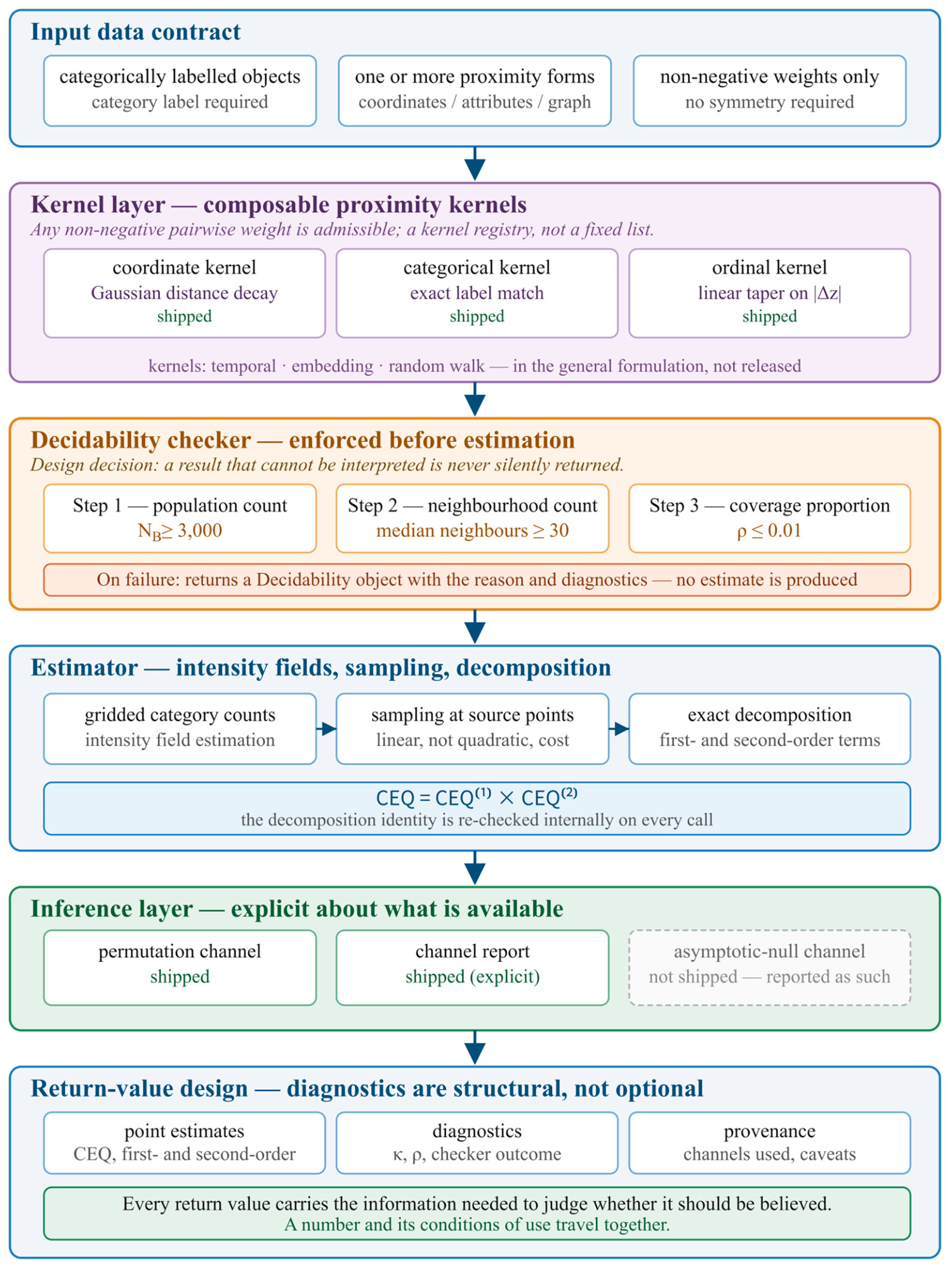
Figure 2.
The three-step decidability check and its failure semantics, together with the population-scale threshold at which the feasible interval closes.
Figure 2.
The three-step decidability check and its failure semantics, together with the population-scale threshold at which the feasible interval closes.
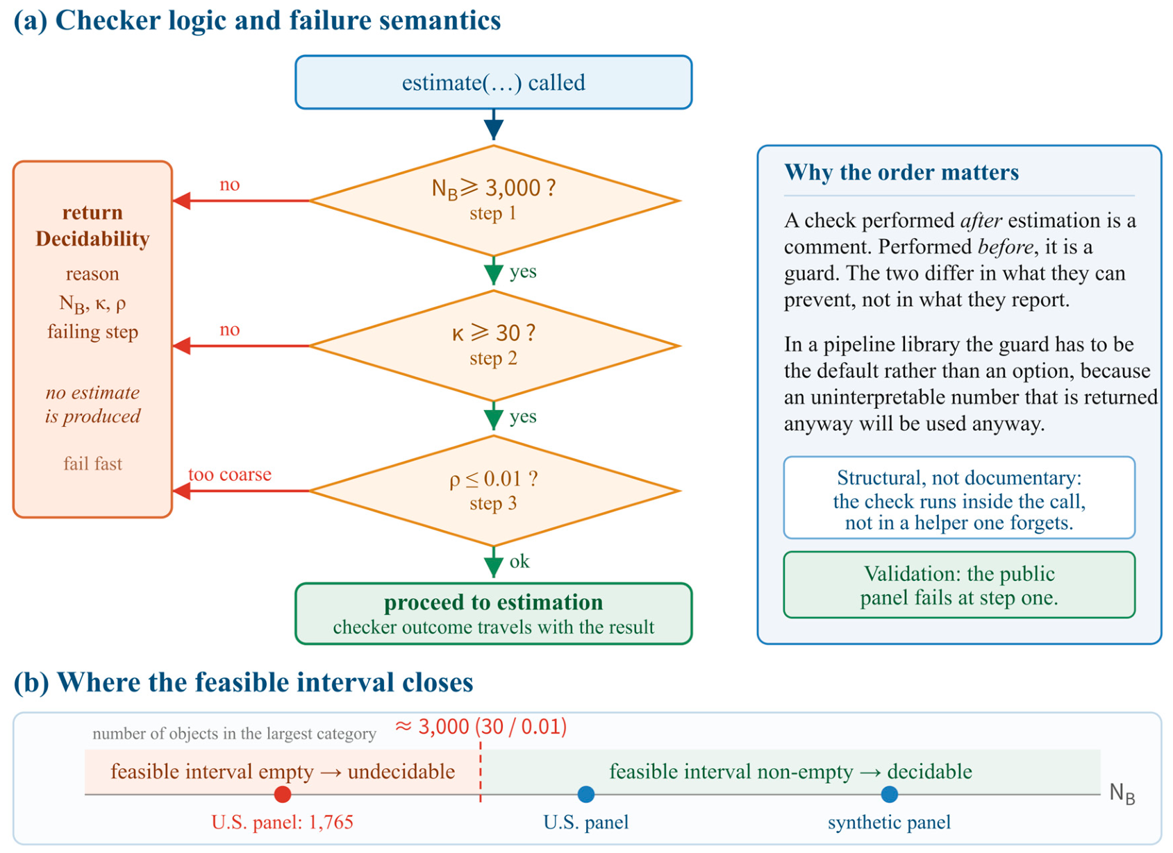
Table 1.
Positioning against related tools.
| Tool or package | Primary data form | Neighbourhood source | Decomposition | Decidability |
|---|---|---|---|---|
| spatstat [12,13] | Spatial point patterns | Geometric | First and second order | No |
| GeoDa [14] | Areal data | Contiguity | Not applicable | No |
| PySAL [15] | Areal data, networks | Contiguity, distance | Not applicable | No |
| STCLQ-Plus [19] | Crime event points | Geometric, temporal | No | No |
| EduCEQ-Toolkit | Any categorically labelled objects | Geometric, attributive | Yes (exact, multiplicative) | Yes (by default) |
Table 2.
Kernel families.
| Family | Component | Form | Parameter | In released code |
|---|---|---|---|---|
| Distance decay | Space | exp(−½(d/b)2), truncated at 3b | Bandwidth b | Yes |
| Ordinal or continuous attribute | Attribute | max(0,1 − |Δz|/r) | Radius r | Yes |
| Categorical attribute | Attribute | 1(zi = zj) | None | Yes |
| Temporal decay | Time | 1/1 + |Δt|, or exp(−|Δt|/τ) | Scale τ | No |
| Radial basis on embedding | Embedding | Temperature σ | No | |
| Random walk | Graph | Weighted sum of adjacency powers | Hops, restart | No |
Table 3.
Module responsibilities.
| Module | Responsibility |
|---|---|
| kernels | Three kernel families (distance, ordinal attribute, categorical attribute), multiplicative composition, degeneracy and collinearity checks |
| estimator | CEQ matrix, first-order and second-order terms, decomposition identity self-check |
| inference | Conditional (stratified) permutation testing, false discovery rate control, explicit channel report |
| diagnostics | Neighbourhood count κ, coverage proportion ρ, the decidability checker returning a Decidability object, spectral-shape check |
| validity | Partial correlation, minimum detectable effect, equivalence testing, proxy attenuation testing, mediation, discrimination decomposition |
Table 4.
The three-step decidability check.
| Step | Input | Output | Criterion | On failure |
|---|---|---|---|---|
| 1 | Labelled object set | Count NB | ≥ 3,000 | Report undecidable, stop |
| 2 | Object set, bandwidth | Median neighbourhood count | ≥ 30 | Suggest larger bandwidth or more data |
| 3 | Object set, bandwidth | Empirical coverage proportion | ≤ 0.01 | Suggest smaller bandwidth |
Table 5.
Default parameters.
| Parameter | Default | Status |
|---|---|---|
| Neighbourhood count threshold | 30 | Convention, changeable |
| Coverage proportion threshold | 0.01 | Convention, changeable |
| Collinearity threshold | 0.7 | Overlap of non-zero supports |
| Permutation count | 999 | Determines p-value resolution |
| FDR method | BH | Switchable to BY under dependency |
| Intensity to pairwise scale ratio | No default | Must be given explicitly |
Table 6.
Bandwidth sweep on the US higher-education panel.
| Bandwidth (km) | κB | ρ | Verdict |
|---|---|---|---|
| 50 | 10.3 | 0.00546 | Undecidable |
| 100 | 23.5 | 0.01376 | Undecidable |
| 150 | 43.5 | 0.02752 | Undecidable |
| 200 | 68.1 | 0.04398 | Undecidable |
| 300 | 119.5 | 0.07960 | Undecidable |
| 400 | 189.0 | 0.13460 | Undecidable |
| 500 | 274.8 | 0.18880 | Undecidable |
Table 9.
Task steps under the conventional workflow and under the present toolkit.
| Step | Manual workflow | Present toolkit |
|---|---|---|
| Construct neighbourhood | Hand-written weight function | Kernel composition, with degeneracy and collinearity checks |
| Check whether data suffice | Usually omitted | Three-step check, executed by default |
| Compute the ratio | Hand-written | estimator.ceq_matrix |
| Separate distribution from interaction | Usually omitted | First-order and second-order decomposition, returned by default |
| Significance | Often global permutation | Conditional (stratified) permutation, strata enforced |
| Multiple comparison | Often omitted | FDR, executed by default |
| When data are insufficient | Returns a number | Returns a statement of non-decidability |
Disclaimer/Publisher’s Note: The statements, opinions and data contained in all publications are solely those of the individual author(s) and contributor(s) and not of MDPI and/or the editor(s). MDPI and/or the editor(s) disclaim responsibility for any injury to people or property resulting from any ideas, methods, instructions or products referred to in the content. |
© 2026 by the authors. Licensee MDPI, Basel, Switzerland. This article is an open access article distributed under the terms and conditions of the Creative Commons Attribution (CC BY) license (http://creativecommons.org/licenses/by/4.0/).
Copyright: This open access article is published under a Creative Commons CC BY 4.0 license, which permit the free download, distribution, and reuse, provided that the author and preprint are cited in any reuse.